LPT-ORSAY/07-12

Abstract

Chiral symmetry breaking may exhibit significantly different patterns in two chiral limits: $N_{f}=2$ massless flavours ($m_{u}=m_{d}=0$, $m_{s}$ physical) and $N_{f}=3$ massless flavours ($m_{u}=m_{d}=m_{s}=0$). Such a difference may arise due to vacuum fluctuations of $s\bar{s}$ pairs related to the violation of the Zweig rule in the scalar sector, and could yield a numerical competition between contributions counted as leading and next-to-leading order in the chiral expansions of observables. We recall and extend Resummed Chiral Perturbation Theory (Re$\chi$PT), a framework that we introduced previously to deal with such instabilities: it requires a more careful definition of the relevant observables and their one-loop chiral expansions. We analyse the amplitudes for low-energy $\pi\pi$ and $\pi K$ scatterings within Re$\chi$PT, which we match in subthreshold regions with dispersive representations obtained from the solutions of Roy and Roy-Steiner equations. Using a frequentist approach, we constrain the quark mass ratio as well as the quark condensate and the pseudoscalar decay constant in the $N_{f}=3$ chiral limit. The results mildly favour significant contributions of vacuum fluctuations suppressing the $N_{f}=3$ quark condensate compared to its $N_{f}=2$ counterpart.

1 Introduction

A striking feature of the Standard Model consists in the mass hierarchy obeyed by the light quarks:

$$m_{u}\sim m_{d}\ll m_{s}\sim\Lambda_{QCD}\ll\Lambda_{H}\,,$$ (1)

where $\Lambda_{QCD}$ is the characteristic scale describing the running of the QCD effective coupling and $\Lambda_{H}\sim 1$ GeV the mass scale of the bound states not protected by chiral symmetry. Therefore, the strange quark may play a special role in the low-energy dynamics of QCD:

i) it is light enough to allow for a combined expansion of observables in powers of $m_{u},m_{d},m_{s}$ around the $N_{f}=3$ chiral limit (meaning 3 massless flavours):

$$N_{f}=3:\qquad m_{u}=m_{d}=m_{s}=0\,,$$ (2)

ii) it is sufficiently heavy to induce significant changes in order parameters from the $N_{f}=3$ chiral limit to the $N_{f}=2$ chiral limit (meaning 2 massless flavours):

$$N_{f}=2:\qquad m_{u}=m_{d}=0\qquad m_{s}{\rm\ physical}\,,$$ (3)

iii) it is too light to suppress efficiently loop effects of massive $\bar{s}s$ pairs (contrary to $c,b,t$ quarks).

These three arguments suggest that $\bar{s}s$ sea pairs may play a significant role in chiral dynamics, leading to different patterns of chiral symmetry breaking in $N_{f}=2$ and $N_{f}=3$ chiral limits. Then, chiral order parameters such as the quark condensate and the pseudoscalar decay constant:

$$\Sigma(N_{f})=-\lim_{N_{f}}\langle\bar{u}u\rangle\,,\qquad\qquad F^{2}(N_{f})=\lim_{N_{f}}F^{2}_{\pi}\,,$$ (4)

would have significantly different values in the two chiral limits ($\lim_{N_{f}}$ denoting the chiral limit with $N_{f}$ massless flavours).

The role of $\bar{s}s$-pairs in the structure of QCD vacuum is a typical loop effect : it should be suppressed in the large-$N_{c}$ limit, and it can be significant only if the Zweig rule is badly violated in the vacuum (scalar) channel $J^{PC}=0^{++}$. On general theoretical grounds [1], one expects $\bar{s}s$ sea-quark pairs to have a paramagnetic effect on chiral order parameters, so that they should decrease when the strange quark mass is sent to zero : for instance, $\Sigma(2;m_{s})\geq\Sigma(2;m_{s}=0)$, and similarly for $F^{2}$, which translates into the paramagnetic inequalities:

$$\Sigma(2)\geq\Sigma(3)\,,\qquad F^{2}(2)\geq F^{2}(3)\,.$$ (5)

However, the size of this paramagnetic suppression is not predicted. Thus, it is highly desirable to extract the size of the chiral order parameters in $N_{f}=2$ and $N_{f}=3$ limits from experiment.

Recent data on $\pi\pi$ scattering [2] together with older data and numerical solutions of the Roy equations [3] allowed us to determine the $N_{f}=2$ order parameters expressed in suitable physical units [4]:

$$X(2) = \frac{(m_{u}+m_{d})\Sigma(2)}{F_{\pi}^{2}M_{\pi}^{2}}=0.81\pm 0.07\,,$$ (6)

$$Z(2) = \frac{F^{2}(2)}{F_{\pi}^{2}}=0.89\pm 0.03\,.$$ (7)

A different analysis of the data in ref. [2], with the additional input of dispersive estimates for the (non-strange) scalar radius of the pion, led to a larger value of $X(2)$ [5]. $X(2)$ and $Z(2)$ seem fairly close to 1, so that corrections related to $m_{u},m_{d}\neq 0$ (while $m_{s}$ remains at its physical value) have a limited impact on the low-energy behaviour of QCD. In turn, two-flavour Chiral Perturbation Theory ($\chi$PT) [6], which consists in an expansion in powers of $m_{u}$ and $m_{d}$ around the $N_{f}=2$ chiral limit, would not suffer from severe problems of convergence .

Two-flavour $\chi$PT [6] deals only with dynamical pions in a very limited range of energy. In order to include $K$- and $\eta$-mesons dynamically and extend the energy range of interest, one must use three-flavour $\chi$PT [9] where the expansion in the three light-quark masses starts around the $N_{f}=3$ vacuum $m_{u}=m_{d}=m_{s}=0$. From the above discussion, large vacuum fluctuations of $\bar{s}s$ pairs would have a dramatic effect on $N_{f}=3$ chiral expansions. The leading-order (LO) term, which depends on the $O(p^{2})$ low-energy constants $F^{2}(3)$ and $\Sigma(3)$, would be damped. On the other hand, next-to-leading-order (NLO) corrections could be enhanced, in particular those related to Zweig-rule violation in the scalar sector. For instance, the Gell-Mann–Oakes–Renner relation would not be saturated by its LO term and would receive sizable numerical contributions from terms counted as NLO in the chiral counting.

Unfortunately, the experimental data on $K$- and $\eta$-decays are not accurate enough to assess the role of $s\bar{s}$ pairs in the $N_{f}$-dependence of chiral symmetry breaking in a very precise way. However our understanding of $\pi K$ scattering at low energies has been improved recently through the re-analysis of dispersive Roy-Steiner equations [10]. A rapid analysis of its results in the framework of three-flavour $\chi$PT hinted at significant vacuum fluctuations encoded in some $O(p^{4})$ chiral couplings, which calls for a more detailed analysis of the $\pi K$ system. Interesting information can also be obtained from our current knowledge of $\pi\pi$ scattering, which we will include in our study.

To perform such an analysis, we develop and modify the framework presented in refs. [1, 11, 12]. Specifically, our work differs from ref. [12] on three points: we consider not only $\pi\pi$- but also $\pi K$-scattering, our observables are the values of the amplitudes in unphysical regions rather than subtraction constants of dispersion relations, the matching between theoretical and experimental representations is performed in a frequentist approach, not in a Bayesian framework.

In sec. 2, we motivate and explain Resummed Chiral Perturbation Theory (Re$\chi$PT), a framework designed to derive three-flavour chiral series at one loop, in which vacuum fluctuations of $s\bar{s}$ pairs are resummed. In sec. 3, we apply Re$\chi$PT to $\pi\pi$- and $\pi K$-scattering amplitudes. In sec. 4, we explain how we determine the same amplitudes dispersively in subthreshold regions, building upon the solutions of Roy and Roy-Steiner equations [3, 10]. In sec. 5, we discuss the matching of the chiral and dispersive results within a frequentist approach [13], and in sec. 6, we present our results for the order parameters of $N_{f}=3$ chiral symmetry breaking. In sec. 7, we summarise and discuss our results. Appendices are devoted to the expression of scattering amplitudes in Re$\chi$PT, their evaluation from Roy and Roy-Steiner equations and the treatment of correlated data.

2 Resummed Chiral Perturbation Theory

We start by describing in more detail the framework introduced in refs. [1, 11, 12] to expand observables around the $N_{f}=3$ chiral limit in the case of significant vacuum fluctuations. We take this opportunity to extend this framework to deal with energy-dependent quantities.

2.1 Convergence of observables

In the introduction, we have emphasised the possibility for three-flavour chiral series to exhibit a rather unusual behaviour, with a numerical competition between leading and next-to-leading order. In ref. [12], we called instability of the expansion such a numerical competition between terms of different chiral counting. A naïve argument based on resonance saturation suggests that higher orders in the chiral expansion should be suppressed by powers of $(F_{\pi}/\Lambda_{H})^{2}$. However, such an argument does not apply to a leading-order contribution proportional to $\Sigma(3)$ [15]: there is no resonance that could saturate the quark condensate. Therefore we expect to encounter three-flavour chiral expansions with a good overall convergence:

$$A=A_{LO}+A_{NLO}+A\delta A\,,\qquad\qquad\delta A\ll 1\,,$$ (8)

but the numerical balance between the leading order $A_{LO}$ and the next-to-leading order $A_{NLO}$ depends on the importance of vacuum fluctuations of $s\bar{s}$ pairs.

At the level of $O(p^{4})$ $N_{f}=3$ chiral perturbation theory, the size of the vacuum fluctuations is encoded in the low-energy constants (LECs) $L_{4}$ and $L_{6}$ whose values remain largely unknown. For a long time [9], they have been set to zero at an arbitrary hadronic scale (typically the $\eta$-mass) assuming that the Zweig rule held in the scalar sector. More recent but indirect analyses based on dispersive methods [10, 17, 18] suggest values of $L_{4}$ and $L_{6}$ which look quite modest but are sufficient to drive the $N_{f}=3$ order parameters $\Sigma(3)$ and $F^{2}(3)$ down to half of their $N_{f}=2$ counterparts $\Sigma(2)$ and $F^{2}(2)$, leading to $A_{LO}\simeq A_{NLO}$ as recalled in sec. 2.3. In addition, two-loop analyses [19, 20, 21, 22] led to values of $L_{4}$ and $L_{6}$ off large-$N_{c}$ expectations.

Unstable $N_{f}=3$ chiral expansions ($A_{LO}\sim A_{NLO}$) demand a more careful treatment than in two-flavour $\chi$PT where such instabilities are seemingly absent. For instance, it would be wrong to believe that the chiral expansion of $1/A$ converges nicely . This might induce the observed problems of convergence in recent two-loop computations [19, 20, 21] : the latter treat the fluctuations encoded in $L_{4}$ and $L_{6}$ as small and are not designed to cope with a large violation of the Zweig rule in the scalar sector, leading to instabilities of the chiral series.

Observables with a good convergence in the sense of eq. (8) form a linear space, which we identify with connected QCD correlators of axial/vector currents and their derivatives, away from kinematic singularities. This choice promotes some “good” observables that can be extracted from such correlators, such as $F_{P}^{2}$ and $F_{P}^{2}M_{P}^{2}$ ($P=\pi,K,\eta$) : LO and NLO may compete, but there should be only a tiny contribution from NNLO and higher orders. On the contrary, the chiral expansion of $M_{P}^{2}$ (ratio of the former quantities) may exhibit a bad convergence. Similarly, the good observable associated with a form factor $F_{P\to Q}$ describing a transition from a pseudoscalar meson $P$ to a meson $Q$ will be $F_{P}F_{Q}F_{P\to Q}$, where the decay constants $F_{P}$ and $F_{Q}$ stem from wave-function renormalisation factors in the LSZ reduction formula.

2.2 One-loop bare expansion of QCD Green functions

In a previous work [12], we proposed a framework to deal with chiral expansions in the case of large fluctuations, by resumming the terms containing the Zweig-rule violating LECs $L_{4}$ and $L_{6}$. This framework, which we will call Resummed Chiral Perturbation Theory (Re$\chi$PT), includes consistently the alternatives of large and small vacuum fluctuations. In this section, we explain how to expand a good observable at one loop in Re$\chi$PT. We addressed only energy-independent quantities in ref. [12], where we explained in detail the similarities and differences of our approach with respect to Generalized Chiral Perturbation Theory [15, 16].

We start from the one-loop generating functional for three-flavour $\chi$PT [9]:

$$Z=Z_{t}+Z_{u}+Z_{A}+\ldots$$ (9)

where the ellipsis stands for NNLO contributions. The three terms of the one-loop generating functional are:

• $Z_{t}$ is the sum of $O(p^{2})$ and $O(p^{4})$ tree graphs, and of tadpole contributions:

  $$Z_{t} = \sum_{P}\int dx\frac{F_{0}^{2}}{6}\left\{1-\frac{3}{16\pi^{2}}\frac{\stackrel{{\scriptstyle\circ}}{{M}}_{P}^{2}}{F_{0}^{2}}\log\frac{\stackrel{{\scriptstyle\circ}}{{M}}_{P}^{2}}{\mu^{2}}\right\}\sigma^{\Delta}_{PP}$$

  $$\quad+\sum_{P}\int dx\frac{3F_{0}^{2}}{6}\left\{1-\frac{3}{6\pi^{2}}\frac{\stackrel{{\scriptstyle\circ}}{{M}}_{P}^{2}}{F_{0}^{2}}\log\frac{\stackrel{{\scriptstyle\circ}}{{M}}_{P}^{2}}{\mu^{2}}\right\}\sigma^{\chi}_{PP}+\int dx\ {\mathcal{L}}_{4}^{r}\,,$$

  where $F_{0}\equiv F(3)$,

  $$F_{0}=F(3)\,,\qquad B_{0}=\frac{\Sigma(3)}{F(3)^{2}}\qquad\,,r=\frac{m_{s}}{m}$$ (11)

  $\sigma^{\Delta}$ and $\sigma^{\chi}$ collect source terms for vector / axial currents and scalar / pseudoscalar densities, and ${\mathcal{L}}_{4}^{r}$ is the $O(p^{4})$ chiral Lagrangian with renormalised couplings $L_{i}^{r}$ and $H_{i}^{r}$. $\stackrel{{\scriptstyle\circ}}{{M}}_{P}^{2}$ denotes the $O(p^{2})$ contribution to the (squared) mass of the Goldstone boson $P$:

  $$\stackrel{{\scriptstyle\circ}}{{M}}_{\pi}^{2}=Y(3)M_{\pi}^{2}\,,\qquad\stackrel{{\scriptstyle\circ}}{{M}}_{K}^{2}=\frac{r+1}{2}Y(3)M_{\pi}^{2}\,,\qquad\stackrel{{\scriptstyle\circ}}{{M}}_{\eta}^{2}=\frac{2r+1}{3}Y(3)M_{\pi}^{2}\,.$$ (12)

• $Z_{u}$ collects unitarity corrections corresponding to one-loop graphs with two $O(p^{2})$ vertices:

  $$Z_{u} = \sum_{P,Q}\int dx\ dy\Big{[}\{\{\partial_{\mu\nu}-g_{\mu\nu}\Box\}M_{PQ}^{r}(x-y)-g_{\mu\nu}L_{PQ}(x-y)\}\hat{\Gamma}^{\mu}_{PQ}(x)\hat{\Gamma}^{\nu}_{QP}(y)$$

  $$\quad-\partial_{\mu}K_{PQ}(x-y)\hat{\Gamma}^{\mu}_{PQ}(x)\bar{\sigma}_{QP}(y)+\frac{1}{4}J^{r}(x-y)\bar{\sigma}_{PQ}(x)\bar{\sigma}_{QP}(y)\Big{]}$$

  where $J,K,L,M$ are (renormalised) functions defined from the one-loop scalar integral with mesons $P$ and $Q$ propagating in the loop, and $\hat{\Gamma}^{\mu}$ and $\bar{\sigma}=\sigma^{\Delta}+\sigma^{\chi}$ collect source terms.

• $Z_{A}$ is the Wess-Zumino functional collecting anomalous contributions.

The one-loop functional eq. (9) has been derived using the propagators and couplings of the $O(p^{2})$ chiral Lagrangian, and therefore it is expressed only in terms of chiral couplings: $F_{0}$ and $B_{0}$, $L_{i}$… [9] In particular, the Goldstone degrees of freedom have masses truncated at $O(p^{2})$, denoted $\stackrel{{\scriptstyle\circ}}{{M}}_{P}^{2}$. Large fluctuations should induce significant differences between this quantity and the physical mass $M_{P}^{2}$. Therefore, we want to replace $\stackrel{{\scriptstyle\circ}}{{M}}_{P}^{2}$ by $M_{P}^{2}$ only when justified by physics arguments, since this replacement may have an important impact when comparing chiral expansions with experimental data.

• The anomalous contribution $Z_{A}$ corresponds to local couplings for vector and axial currents, and is not affected by our discussion.

• For the unitarity corrections $Z_{u}$, were we to consider higher and higher orders of the chiral expansion, we should obtain that the masses occurring in the functions $J^{r}$, $K$, $L$ and $M^{r}$ are physical masses, in order to get the low-mass two-particle cuts at the physical positions. Therefore, we write those functions with the physical masses of the Goldstone bosons. On the contrary, we keep the multiplying factors $\Gamma^{\mu}$ and $\bar{\sigma}$ expressed in terms of parameters of the effective Lagrangian ($m_{q}$, $B_{0}$…).

• The tadpole contributions present in $Z_{t}$ are derived using the $O(p^{2})$ contribution to the Goldstone boson masses $\stackrel{{\scriptstyle\circ}}{{M}}_{P}^{2}$. In ref. [12], we have proposed the replacement:

  $$\frac{\stackrel{{\scriptstyle\circ}}{{M}}_{P}^{2}}{32\pi^{2}}\log\frac{\stackrel{{\scriptstyle\circ}}{{M}}_{P}^{2}}{\mu^{2}}\quad\to\quad\frac{\stackrel{{\scriptstyle\circ}}{{M}}_{P}^{2}}{32\pi^{2}}\log\frac{M_{P}^{2}}{\mu^{2}}\,.$$ (14)

  We could have kept $\stackrel{{\scriptstyle\circ}}{{M}}_{P}^{2}$ everywhere in $Z_{t}$, and in particular inside the logarithm. However, the resulting expressions are easier to deal with, and the change has only a tiny numerical impact: either $M_{P}$ is close to its $O(p^{2})$ term and the change is trivially justified, or $\stackrel{{\scriptstyle\circ}}{{M}}_{P}^{2}$ is much smaller than $M_{P}^{2}$ and the whole tadpole contribution is very small.

• Physical $S$-matrix elements are obtained from the Green functions derived with the generating functional by applying the LSZ reduction formula. The external legs corresponding to incoming and outgoing particles must be put on the mass shell. In the process, the products of external momenta are translated into the well-known Mandelstam variables. These kinematical relations are valid for physical masses, and we will use the latter (and not the $O(p^{2})$ truncated masses $\stackrel{{\scriptstyle\circ}}{{M}}_{P}^{2}$) whenever we reexpress products of external momenta. This prescription is consistent with the use of physical masses in the one-loop scalar integral present in the unitarity term $Z_{u}$.

Following the renormalisation procedure in ref. [9], one can check easily that eq. (14) does not change the renormalisation-scale dependence of LECs at one loop. Actually, the whole one-loop generating functional $Z$ becomes exactly renormalisation-scale independent : when we follow the prescription given above, all the scale-dependent logarithms present in $Z_{t}$ (explictly shown in eq. (• ‣ 2.2)) and $Z_{u}$ (hidden in the one-loop functions $M^{r}$ and $J^{r}$ in eq. (• ‣ 2.2)) are multiplied by terms of the same form $m_{q}B_{0}$ and thus cancel exactly. In the more usual treatment of the tadpoles [9], $m_{q}B_{0}$ terms are replaced by physical Goldstone masses in the one-loop generating functional (see sec. 8 in ref. [9]). In this case, the cancellation of the logarithms takes place only up to $O(p^{4})$ and some higher-order logarithmic pieces of $Z_{t}$ have no counterpart in $Z_{u}$.

We call “bare expansion” the chiral expansion treated according to our prescription, because of we prefer keeping original couplings of the chiral Lagrangian to trading them for physical masses and decay constants. We sum up our method to obtain bare expansions of Green functions in Resummed $\chi$PT:

1. Consider a subset of observables suitable for a chiral expansion, such as the linear space of connected QCD correlators of axial/vector currents and their derivatives away from kinematic singularities.

2. Extract the bare expansion of the observables using the one-loop generating functional eq. (9): in $Z_{t}$, replace the tadpole contributions by eq. (14), and in $Z_{u}$, use the physical masses for the functions $J,K,L,M$ defined from the one-loop scalar integral.

3. Use physical masses to reexpress scalar products of external momenta in terms of the Mandelstam variables.

4. Keep track of the higher-order contributions by introducing remainders, i.e. NNLO quantities which have an unknown value but are assumed small enough for the chiral series to converge.

5. Exploit algebraically the resulting relations, and never trade the couplings of the chiral Lagrangian for observables while neglecting higher-order terms.

The main differences from the usual treatment of three-flavour chiral series consists in the choice of a particular subset of observables, the distinction between physical meson masses and their $O(p^{2})$ truncated forms, and the algebraic use of chiral expansions while keeping track of higher-order terms explicitly.

2.3 Masses and decay constants of Goldstone bosons

The first example consists in pseudoscalar decay constants and masses. The usual $\chi$PT expressions (Sec. 10 in ref. [9]) become the following bare expansions in Re$\chi$PT (similar expressions for $\eta$ can be found in refs. [12, 25]):

$$F_{\pi}^{2} = F_{\pi}^{2}Z(3)+8(r+2)Y(3)M_{\pi}^{2}\Delta L_{4}+8Y(3)M_{\pi}^{2}\Delta L_{5}+F_{\pi}^{2}e_{\pi}\,,$$ (15)

$$F_{K}^{2} = F_{\pi}^{2}Z(3)+8(r+2)Y(3)M_{\pi}^{2}\Delta L_{4}+4(r+1)Y(3)M_{\pi}^{2}\Delta L_{5}+F_{K}^{2}e_{K}\,,$$ (16)

$$F_{\pi}^{2}M_{\pi}^{2} = F_{\pi}^{2}M_{\pi}^{2}X(3)+16(r+2)Y^{2}(3)M_{\pi}^{4}\Delta L_{6}+16Y^{2}(3)M_{\pi}^{4}\Delta L_{8}+F_{\pi}^{2}M_{\pi}^{2}d_{\pi}\,,$$ (17)

$$F_{K}^{2}M_{K}^{2} = \frac{r+1}{2}F_{\pi}^{2}M_{\pi}^{2}X(3)$$

$$\qquad+8(r+2)(r+1)Y^{2}(3)M_{\pi}^{4}\Delta L_{6}+4(r+1)^{2}Y^{2}(3)M_{\pi}^{4}\Delta L_{8}+F_{K}^{2}M_{K}^{2}d_{K}\,,$$

We take as free parameters the $N_{f}=3$ quark condensate and pseudoscalar decay constant expressed in physical units , as well as their ratio and the quark mass ratio:

$$X(3)=\frac{2m\Sigma(3)}{F_{\pi}^{2}M_{\pi}^{2}}\,,\quad Z(3)=\frac{F^{2}(3)}{F_{\pi}^{2}}\,,\quad Y(3)=\frac{X(3)}{Z(3)}=\frac{2mB_{0}}{M_{\pi}^{2}}\,,r=\frac{m_{s}}{m}$$ (19)

We have introduced the NNLO remainders $d_{\pi}$, $e_{\pi}$, $d_{K}$ and $e_{K}$, and the combinations of LECs and chiral logarithms:

$$\Delta L_{4} = L_{4}^{r}(\mu)-\frac{1}{256\pi^{2}}\log\frac{M_{K}^{2}}{\mu^{2}}$$ (20)

$$\quad+\frac{1}{128\pi^{2}}\frac{r}{(r-1)(r+2)}\left\{\log\frac{M_{K}^{2}}{M_{\pi}^{2}}+\left(1+\frac{1}{2r}\right)\log\frac{M_{\eta}^{2}}{M_{\pi}^{2}}\right\}\,,$$

$$\Delta L_{5} = L_{5}^{r}(\mu)-\frac{1}{256\pi^{2}}\left[\log\frac{M_{K}^{2}}{\mu^{2}}+2\log\frac{M_{\eta}^{2}}{\mu^{2}}\right]$$ (21)

$$\quad-\frac{1}{256\pi^{2}(r-1)}\left(3\log\frac{M_{\eta}^{2}}{M_{K}^{2}}+5\log\frac{M_{K}^{2}}{M_{\pi}^{2}}\right)\,.$$

$$\Delta L_{6} = L_{6}^{r}(\mu)-\frac{1}{512\pi^{2}}\left(\log\frac{M_{K}^{2}}{\mu^{2}}+\frac{2}{9}\log\frac{M_{\eta}^{2}}{\mu^{2}}\right)$$ (22)

$$\quad+\frac{1}{512\pi^{2}}\frac{r}{(r+2)(r-1)}\left(3\log\frac{M_{K}^{2}}{M_{\pi}^{2}}+\log\frac{M_{\eta}^{2}}{M_{K}^{2}}\right)\,.$$

$$\Delta L_{8} = L_{8}^{r}(\mu)-\frac{1}{512\pi^{2}}\left[\log\frac{M_{K}^{2}}{\mu^{2}}+\frac{2}{3}\log\frac{M_{\eta}^{2}}{\mu^{2}}\right]$$ (23)

$$\quad-\frac{1}{512\pi^{2}(r-1)}\left(3\log\frac{M_{K}^{2}}{M_{\pi}^{2}}+\log\frac{M_{\eta}^{2}}{M_{K}^{2}}\right)\,,$$

The values of the logarithms are only mildly dependent on $r$; for $r=25$,

$$\Delta L_{4}=L_{4}^{r}(M_{\rho})+0.51\cdot 10^{-3}\,, \Delta L_{5}=L_{5}^{r}(M_{\rho})+0.67\cdot 10^{-3}\,,$$ (24)

$$\Delta L_{6}=L_{6}^{r}(M_{\rho})+0.26\cdot 10^{-3}\,, \Delta L_{8}=L_{8}^{r}(M_{\rho})+0.20\cdot 10^{-3}\,.$$ (25)

Since $F_{\pi}$, $F_{K}$, $M_{\pi}$ and $M_{K}$ are accurately known, we can use these expressions to eliminate some of the $O(p^{4})$ LECs in the chiral expansion of other observables. This is rather different from the usual $\chi$PT trading, since we keep explicitly higher-order terms that would have been neglected in the usual (perturbative) treatment of chiral series.

From the masses and decay constants (15)-(2.3), we get the equivalent set of equations providing some $O(p^{4})$ LECs in terms of physical masses and decay constants, $r,X(3),Y(3)$ and NNLO remainders:

$$Y^{2}(3)\Delta L_{6} = \frac{1}{16(r+2)}\frac{F_{\pi}^{2}}{M_{\pi}^{2}}[1-\epsilon(r)-X(3)-d]\,,$$ (26)

$$Y^{2}(3)\Delta L_{8} = \frac{1}{16}\frac{F_{\pi}^{2}}{M_{\pi}^{2}}[\epsilon(r)+d^{\prime}]\,,$$ (27)

$$Y(3)\Delta L_{4} = \frac{1}{8(r+2)}\frac{F_{\pi}^{2}}{M_{\pi}^{2}}[1-\eta(r)-Z(3)-e]\,,$$ (28)

$$Y(3)\Delta L_{5} = \frac{1}{8}\frac{F_{\pi}^{2}}{M_{\pi}^{2}}[\eta(r)+e^{\prime}]\,.$$ (29)

with

$$\epsilon(r)=2\frac{r_{2}-r}{r^{2}-1},\qquad\eta(r)=\frac{2}{r-1}\left(\frac{F_{K}^{2}}{F_{\pi}^{2}}-1\right)\,,$$ (30)

and the following linear combinations of NNLO remainders arise:

$$d = \frac{r+1}{r-1}d_{\pi}-\left(\epsilon(r)+\frac{2}{r-1}\right)d_{K}\,,\qquad d^{\prime}=d-d_{\pi}\,,$$ (31)

$$e = \frac{r+1}{r-1}e_{\pi}-\left(\eta(r)+\frac{2}{r-1}\right)e_{K}\,,\qquad e^{\prime}=e-e_{\pi}\,.$$ (32)

The above identities are algebraically exact, but they are useful only as long as NNLO remainders are small. In refs. [12, 25], the size of the NNLO remainders was taken as

$$d,e=O(m_{s}^{2})\sim 10\%\,,\qquad d^{\prime},e^{\prime}=O(mm_{s})\sim 3\%\,,$$ (33)

with the rule of thumb that NNLO corrections of size $O(m_{s}^{2})$ should not exceed $(30\%)^{2}\simeq 10\%$ of the contribution to the observable while $O(m_{s}m)$ terms would be less than $30\%\cdot 10\%\simeq 3\%$. We will propose in the next section a different but compatible way of dealing with this issue.

In eqs. (26)-(29), the presence of powers of $Y(3)$, i.e., $B_{0}$, follows from the normalisation of the scalar and pseudoscalar sources in ref. [9]: these powers arise only for $O(p^{4})$ LECs related to explicit chiral symmetry breaking (two powers for $L_{6},L_{7},L_{8}$, one for $L_{4}$ and $L_{5}$), and are absent for LECs associated with purely derivative terms.

2.4 From bare expansions to Re$\chi$PT expansions

As shown in detail in ref. [11], plugging eqs. (26)-(29) into the bare expansions for other observables corresponds to resumming the vacuum fluctuations encoded in $L_{4}$ and $L_{6}$. As an illustration, we recall that we can exploit eqs. (26)-(29) to relate $Y(3)$ to the chiral couplings $L_{4}$ and $L_{6}$:

$$Y(3) = \frac{2[1-\epsilon(r)-d]}{\displaystyle[1-\eta(r)-e]+\sqrt{[1-\eta(r)-e]^{2}+k\times[2\Delta L_{6}-\Delta L_{4}]}}\,,$$ (34)

$$k = 32(r+2)\frac{M_{\pi}^{2}}{F_{\pi}^{2}}[1-\epsilon(r)-d]\,.$$ (35)

If vacuum fluctuations are small, i.e. $\Delta L_{6}$ and $\Delta L_{4}$ almost vanishing, one can treat $k\times[2\Delta L_{6}-\Delta L_{4}]$ in the denominator as a small perturbation and linearise the equation as $Y(3)=1+O(p^{2})$. This corresponds to the usual (iterative and perturbative) treatment of chiral series. However the factor $k$ is very large ($k\simeq 1900$ for $r=25$) and values of $\Delta L_{6}$ and $\Delta L_{4}$ of a few $10^{-3}$ suffice to yield an important deviation of $Y(3)$ from 1, while the linear approximation becomes inaccurate. Similar relations exist between $X(3)$ and $\Delta L_{6}$, and between $Z(3)$ and $\Delta L_{4}$ [11].

Using eqs. (26)-(29), we obtain the one-loop expansions of good observables in Re$\chi$PT, by using eqs. (26)-(29) and reexpressing $F(3)$, $mB_{0}$, $Y(3)L_{4}$, $Y(3)L_{5}$, $Y(3)^{2}L_{6}$, $Y(3)^{2}L_{8}$ (and $Y(3)^{2}L_{7}$ through $\eta$ identities) in terms of the three parameters of interest $X(3)$, $Z(3)$, $r$ and NNLO remainders. In the case of $\pi\pi$ and $\pi K$ scatterings, only three $O(p^{4})$ LECs ($L_{1},L_{2},L_{3}$) will remain. The square root induced by equations like eq. (34) is a non-perturbative feature of our framework. It amounts to resumming (potentially) large contributions of vacuum fluctuations, encoded in the Zweig-rule violating LECs $L_{4}$ and $L_{6}$. This feature, contrasting with the usual treatment of chiral series, has led us to call our framework Resummed Chiral Perturbation Theory or Re$\chi$PT.

There is a price to pay for this extension of the chiral framework in the case of large fluctuations of $s\bar{s}$ pairs, and the resulting competition between LO and NLO in the chiral counting: some usual $O(p^{4})$ relations cannot be exploited anymore, because of our ignorance about their convergence. For instance, the quark mass ratio $r=m_{s}/m$ ($m=m_{u}=m_{d}$) cannot be fixed from $M_{K}^{2}/M_{\pi}^{2}$ since we do not control the convergence of its three-flavour chiral expansion. $r$ becomes a free parameter which can vary in the range:

$$r_{1}=2\frac{F_{K}M_{K}}{F_{\pi}M_{\pi}}-1\sim 8\leq r\leq r_{2}=2\frac{F_{K}^{2}M_{K}^{2}}{F_{\pi}^{2}M_{\pi}^{2}}-1\sim 36\,.$$ (36)

Similarly, one cannot determine LECs or combinations of LECs through ratios of observables. For instance, one should not use $F_{K}/F_{\pi}$ to determine $L_{5}$ at $O(p^{4})$, because we do not know if the chiral expansion of $F_{K}/F_{\pi}$ converges at all. Finally, the agreement of the pseudoscalar spectrum with the Gell-Mann–Okubo formula requires a fine tuning of $L_{7}$ (however, this fine tuning is also needed in the case of a dominant $N_{f}=3$ quark condensate and small vacuum fluctuations [12]).

3 $\pi\pi$ and $\pi K$ scattering amplitudes

In this section, we are applying the Re$\chi$PT framework to two examples of Goldstone-boson scatterings : $\pi\pi$ scattering, which probes the structure of QCD vacuum in the $N_{f}=2$ chiral limit, and $\pi K$ scattering, which is linked with the $N_{f}=3$ chiral limit.

3.1 One-loop expression in Re$\chi$PT

In the isospin symmetry limit, the low-energy $\pi\pi$ scattering is described by a single Lorentz-invariant amplitude:

$$A(\pi^{a}(p_{1})+\pi^{b}(p_{2})\to\pi^{c}(p_{3})+\pi^{d}(p_{4}))=\delta^{ab}\delta^{cd}A(s,t,u)+\delta^{ac}\delta^{bd}A(t,u,s)+\delta^{ad}\delta^{bc}A(u,t,s)\,$$ (37)

where the usual Mandelstam variables are:

$$s=(p_{1}+p_{2})^{2}\,,\qquad t=(p_{1}-p_{3})^{2}\,,\qquad u=(p_{1}-p_{4})^{2}\,,$$ (38)

and $A$ is symmetric under $t\leftrightarrow u$ exchange. In a similar way, we consider the low-energy $\pi K$ scattering, which can be decomposed into two amplitudes according to isospin in the $s$-channel $I=3/2$ and $I=1/2$:

$$A(\pi^{a}(p_{1})+K^{i}(p_{2})\to\pi^{b}(p_{3})+K^{j}(p_{4}))=F^{I}_{\pi K}(s,t,u)\,,$$ (39)

from which one can define two amplitudes, respectively even and odd under $s\leftrightarrow u$ exchange:

$$B(s,t,u) = \frac{2}{3}F^{3/2}_{\pi K}(s,t,u)+\frac{1}{3}F^{1/2}_{\pi K}(s,t,u)\,,$$ (40)

$$C(s,t,u) = -\frac{1}{3}F^{3/2}_{\pi K}(s,t,u)+\frac{1}{3}F^{1/2}_{\pi K}(s,t,u)\,.$$ (41)

In addition, crossing symmetry provides a relation between the two amplitudes:

$$F^{1/2}_{\pi K}(s,t,u)=\frac{3}{2}F^{3/2}_{\pi K}(u,t,s)-\frac{1}{2}F^{3/2}_{\pi K}(s,t,u)\,.$$ (42)

We can apply the prescriptions described in sec. 2.2 to determine the one-loop Re$\chi$PT expansions of $A$, $B$ and $C$. The relevant good observables, which can be derived from Green functions of vector/axial currents, are $F_{\pi}^{4}A$, $F_{\pi}F_{K}F$ and $F_{\pi}F_{K}G$.

1. We determine the one-loop bare expansions of these quantities. This can be done using the generating functional of $N_{f}=3$ $\chi$PT [9], with the essential difference that we keep the distinction between $O(p^{2})$ truncated masses and physical masses of the Goldstone bosons. This was performed in the case of $\pi K$ scattering in ref. [26]. A similar work can be done in the case of $\pi\pi$ scattering. The corresponding (rather lengthy) expressions are summarised in app. A.

2. We use eqs. (20)-(23) to reexpress the $O(p^{4})$ LECs $L_{4}$, $L_{5}$, $L_{6}$, $L_{8}$ in terms of $r$, $X(3)$ and $Z(3)$, and NNLO remainders related to $\pi$ and $K$ masses and decay constants. We denote with the superscript ${LO+NLO}$ the resulting expressions, which include the LO and NLO expansions of the relevant good observables and resum the vacuum fluctuations encoded in $L_{4}$ and $L_{6}$.

3. To obtain the Re$\chi$PT expansions of the $\pi\pi$ and $\pi K$ scattering amplitudes, we add to the resulting expressions a polynomial modeling higher-order contributions :

   $$F_{\pi}^{4}A^{Re\chi PT} = F_{\pi}^{4}A^{LO+NLO}+F_{\pi}^{2}(s_{A}-M_{\pi}^{2})a_{1}+F_{\pi}^{2}(s-s_{A})a_{2}$$

   $$\qquad+(s-s_{A})^{2}a_{3}+[(t-t_{A})^{2}+(u-u_{A})^{2}]a_{4}\,,$$

   $$F_{\pi}^{2}F_{K}^{2}B^{Re\chi PT} = F_{\pi}^{2}F_{K}^{2}B^{LO+NLO}+F_{\pi}F_{K}t_{B}b_{1}+F_{\pi}F_{K}(t-t_{B})b_{2}$$

   $$\qquad+(t-t_{B})^{2}b_{3}+[(s-s_{B})^{2}+(u-u_{B})^{2}]b_{4}\,,$$

   $$F_{\pi}^{2}F_{K}^{2}C^{Re\chi PT} = F_{\pi}^{2}F_{K}^{2}C^{LO+NLO}+F_{\pi}F_{K}(s-u)c_{1}+(t-t_{B})(s-u)c_{2}\,,$$ (45)

   where $(s_{A},t_{A},u_{A})$, $(s_{B},t_{B},u_{B})$, $(s_{C},t_{C},u_{C})$ denote the points around which we perform the expansion of the NNLO polynomial. The first remainder is multiplied by a constant estimating roughly the value of the amplitude at the expansion point (obtained from the LO chiral expression). The other remainders are multiplied by polynomials in the Mandelstam variables which vanish at the expansion point and respect the crossing properties of the amplitude.

For our purposes, we take:

$$(s_{A},t_{A},u_{A}) = (4/3M_{\pi}^{2},4/3M_{\pi}^{2},4/3M_{\pi}^{2})\,,$$ (46)

$$(s_{B},t_{B},u_{B}) = (s_{C},t_{C},u_{C})=(M_{K}^{2}+1/3M_{\pi}^{2},4/3M_{\pi}^{2},M_{K}^{2}+1/3M_{\pi}^{2})\,.$$ (47)

The remainders $a_{i},b_{i},c_{i}$ include only NNLO terms or higher : we expect therefore these contributions to be suppressed by $1/\Lambda_{H}^{4}$ where $\Lambda_{H}$ is a typical hadronic scale [27]. On the other hand, the numerator may depend on the remainder considered, but the contribution to the polynomial must be order $O(p^{6})$ in the usual chiral counting. This means that the remainders have a typical size of order:

$$a_{1},a_{2},b_{1},b_{2},c_{1}\sim\frac{M_{K}^{4}}{\Lambda_{H}^{4}}\,,\qquad a_{3},a_{4},b_{3},b_{4},c_{2}\sim\frac{F_{\pi}^{2}M_{K}^{2}}{\Lambda_{H}^{4}}\,.$$ (48)

Remainders associated with higher-order polynomials would be of order $F_{\pi}^{4}/\Lambda_{H}^{4}$, much suppressed compared to the terms considered here, and thus neglected in the following analysis.

In the case of $\pi\pi$ scattering, we can exploit the behaviour of the amplitude in the $N_{f}=2$ chiral limit in order to constrain the size of NNLO remainders further. Indeed, from $N_{f}=2$ chiral perturbation theory, we know that:

$$F_{\pi}^{4}A(s,t,u)-F_{\pi}^{2}(s-M_{\pi}^{2})=O(\epsilon^{4})\quad{\rm with}\quad\epsilon^{2}\sim p^{2}\sim m\,.$$ (49)

$\epsilon$ counts only powers of $m=m_{u}=m_{d}$ but not those of $m_{s}$. If we compare this relation with $F_{\pi}^{4}A$ expressed in $N_{f}=3$ Re$\chi$PT in eqs. (3) and (A.1), we see that the relation (49) implies a constrain on the NNLO remainders : $a_{1}-e_{\pi}-(d_{\pi}-e_{\pi})/3/(s_{A}/M_{\pi}^{2}-1)$ and $a_{2}-e_{\pi}$ must be proportional to $m$. Therefore, we can expect the remainders to exhibit the typical sizes:

$$a_{1}-e-\frac{d-e}{3(s_{A}/M_{\pi}^{2}-1)},a_{2}-e\sim\frac{M_{\pi}^{2}M_{K}^{2}}{\Lambda_{H}^{4}}\,,\qquad b_{1},b_{2},c_{1}\sim\frac{M_{K}^{4}}{\Lambda_{H}^{4}}\,,\qquad a_{3},a_{4},b_{3},b_{4},c_{2}\sim\frac{F_{\pi}^{2}M_{K}^{2}}{\Lambda_{H}^{4}}\,.$$ (50)

According to this discussion, we take the following ranges for the direct remainders:

$$a_{1}-e-\frac{F_{\pi}^{2}M_{\pi}^{2}}{3(s_{A}-M_{\pi}^{2})}(d-e),a_{2}-e\in\left[-\frac{2M_{\pi}^{2}M_{K}^{2}}{\Lambda_{H}^{4}},\frac{2M_{\pi}^{2}M_{K}^{2}}{\Lambda_{H}^{4}}\right]\,,$$ (51)

$$b_{1},b_{2},c_{1}\in\left[-\frac{M_{K}^{4}}{\Lambda_{H}^{4}},\frac{M_{K}^{4}}{\Lambda_{H}^{4}}\right]\,,\qquad a_{3},a_{4},b_{3},b_{4},c_{2}\in\left[-\frac{F_{\pi}^{2}M_{K}^{2}}{\Lambda_{H}^{4}},\frac{F_{\pi}^{2}M_{K}^{2}}{\Lambda_{H}^{4}}\right]\,,$$

with $\Lambda_{H}=0.85$ GeV. This choice for the numerical value of $\Lambda_{H}$ provides a good agreement of our estimates with those used in refs. [1, 4, 12] for energy-independent quantities. In the latter references, NNLO remainders were taken of order $O(m_{s}^{2})=(30\%)^{2}=10\%$ of the leading-order value, unless they were suppressed by one power of $m$ and thus of order $O(mm_{s})=30\%\times 10\%=3\%$. According to this work, the same remainders must remain respectively of order $M_{K}^{4}/\Lambda_{H}^{4}=12\%$ and $2M_{\pi}^{2}M_{K}^{2}/\Lambda_{H}^{4}=2\%$. In addition, one can check that the definition and size of remainders given in this section can be applied to the two-point correlators related to $F_{P}^{2}$ and $F_{\pi}^{2}M_{\pi}^{2}$ with an expansion around the point of vanishing transfer momentum, leading to remainders identical to those defined in sec. 2.3.

3.2 Roy and Roy-Steiner equations

The above theoretical expressions for low-energy $\pi\pi$ and $\pi K$ scattering must be compared to experimental information in order to extract the parameters of three-flavour chiral symmetry breaking. Fortunately, dispersion relations provide an appropriate framework to analyse experimental data and extract the low-energy behaviour of the amplitude, through Roy and Roy-Steiner equations.

In ref. [3], Roy equations were derived and solved with experimental input on high-energy $\pi\pi$ scattering. The solutions were parametrised in terms of two scattering lengths $a_{0}^{0}$ and $a_{0}^{2}$. In refs. [3] and [4], these solutions, and some of their extensions, were exploited together with recent data on $\pi\pi$ scattering in order to determine the low-energy structure of the amplitude with the best accuracy. Ref. [5] proposed to combine $K_{\ell 4}$ data on $\delta_{0}^{0}-\delta_{1}^{1}$ supplemented with a theoretical constraint from the scalar radius of the pion. This constraint was assessed critically in ref. [4], where it was proposed to avoid any reference to the scalar radius of the pion and to rely only on experimental data, namely $K_{\ell 4}$ data supplemented with $I=2$ data. We follow the latter approach and take the results of the so-called “Global” fit, eq. (12) in ref. [4], for $\pi\pi$-scattering data.

In ref. [10], Roy-Steiner equations were investigated to study the $\pi K$ scattering amplitude. In spite of recent progress in $\tau\to K\pi\nu_{\tau}$ and $D\to K\pi e\nu_{e}$ decays, low-energy data on $\pi K$ phase shifts is still lacking. However the dispersive analysis of the data in the intermediate region turned out to provide rather tight constrains on the low-energy $\pi K$ amplitude. We use the results of ref. [10] for $\pi K$ scattering.

It is a straightforward, if tedious, exercise, to exploit the dispersive representations of the amplitudes $A$,$B$,$C$ found in sec. 3 of ref. [3] and in sec. 2 of ref. [10], and to compute them in subthreshold regions, where none of the dispersion integrals exhibit singularities. We checked in particular that our representation of the low-energy $\pi K$ amplitude was in good numerical agreement with the subthreshold expansion presented in sec. 6.3 in ref. [10].

We define the subthreshold region of interest for $\pi\pi$ scattering as a triangle in the Mandelstam plane delimited by points with $(s,t,u)$:

$$(2M_{\pi}^{2},M_{\pi}^{2},M_{\pi}^{2})\,,\qquad(M_{\pi}^{2}/2,3/2M_{\pi}^{2},3/2M_{\pi}^{2})\,,\qquad(M_{\pi}^{2}/2,3M_{\pi}^{2},M_{\pi}^{2}/2)\,,$$ (52)

taking into account the symmetry of the amplitude under $t-u$ exchange. Similarly, we define for $\pi K$ scattering a triangle in the Mandelstam plane with:

$$(M_{K}^{2},2M_{\pi}^{2},M_{K}^{2})\,,\qquad(M_{K}^{2},0,M_{K}^{2}+2M_{\pi}^{2})\,,\qquad(M_{K}^{2}+M_{\pi}^{2},0,M_{K}^{2}+M_{\pi}^{2})\,,$$ (53)

exploiting the symmetry or antisymmetry under $s-u$ exchange. In each triangle, we defined 15 points regularly spaced where we compute the scattering amplitudes. Some aspects of the computation, and of the correlations among the points, are covered in app. B.

4 Matching in a frequentist approach

We must match the chiral expansions of the scattering amplitudes with the experimental values described in the previous section. We perform this matching in a frequentist approach inspired by the Rfit method [13].

4.1 Likelihood

We collect in a vector $V$ our $3n$ observables :

$$V^{T}=\left[A(s_{1},t_{1}),\ldots A(s_{n},t_{n}),B(s^{\prime}_{1},t^{\prime}_{1}),\ldots B(s^{\prime}_{n},t^{\prime}_{n}),C(s^{\prime\prime}_{1},t^{\prime\prime}_{1}),\ldots C(s^{\prime\prime}_{n},t^{\prime\prime}_{n})\right]\,.$$ (54)

Since we use the masses and decay constant identities for pions and kaons to reexpress the $O(p^{4})$ LECs in terms of $F_{P}^{2}$ and $F_{P}^{2}M_{P}^{2}$ through eqs. (26)-(29), our set of theoretical parameters is:

$${\rm Parameters} : r,X(3),Z(3),L_{1}^{r},L_{2}^{r},L_{3}\,,$$ (55)

$${\rm Direct\ remainders} : a_{1},a_{2},a_{3},a_{4},b_{1},b_{2},b_{3},b_{4},c_{1},c_{2}\,,$$ (56)

$${\rm Indirect\ remainders} : d,d^{\prime},e,e^{\prime},d_{X},d_{Z}\,.$$ (57)

We have separated the direct remainders, attached to the bare expansions of the observables, and the indirect remainders, arising through the reexpression of $O(p^{4})$ LECs thanks to mass and decay constant equalities. The latter include also the remainders $d_{X}$ and $d_{Z}$, whose expressions will be given in sec. 4.2 and which are required to express the paramagnetic constraints on $X$ and $Z$, eq. (5).

We construct the experimental likelihood ${\mathcal{L}}_{\rm exp}$, i.e. the probability of observing the data for a given choice of theoretical parameters $T_{n}$ :

$${\mathcal{L}}_{\rm exp}(T_{n})=P({\rm data}|T_{n})\propto\exp\left(-\frac{1}{2}(V_{th}-V_{exp})^{T}C^{-1}(V_{th}-V_{exp})\right)/\sqrt{\det C}\,.$$ (58)

To avoid a proliferation of (purely numerical) normalisation factors of no significance for our discussion, we use the sign $\propto$ meaning “proportional to”. $C$ is the covariance matrix between the experimental values $V_{exp}$ computed through eq. (82), whereas $V_{th}$ denote the theoretical values computed with the particular choice of $T_{n}$. Since we expect strong correlations among the parameters, the covariance matrix must be treated with some care, as described in app. C.

The theoretical likelihood ${\mathcal{L}}_{\rm th}(T_{n})$ describes our current knowledge on the theory parameters. In agreement with the Rfit prescription [13], we consider that ${\mathcal{L}}_{\rm th}(T_{n})=1$ if each theoretical parameter lies within its allowed range described in the next section, otherwise the likelihood vanishes.

4.2 Constraints on the theoretical parameters

To build the theoretical likelihood, we impose a list of constraints on the theoretical parameters. Some constraints are fairly simple:

• We take the following range for the ratio of quark masses $r$:

  $$r_{1}\leq r\leq r_{2}\,,\qquad r_{1}=2\frac{F_{K}M_{K}}{F_{\pi}M_{\pi}}-1\,,\qquad r_{2}=2\left(\frac{F_{K}M_{K}}{F_{\pi}M_{\pi}}\right)^{2}-1\,.$$ (59)

• Vacuum stability yields constraints on the $N_{f}=3$ chiral order parameters:

  $$X(3)\geq 0\,,\qquad Z(3)\geq 0\,.$$ (60)

• We allow the three $O(p^{4})$ LECs $L_{1}^{r}(M_{\rho}),L_{2}^{r}(M_{\rho}),L_{3}$ in the range $[-F_{\pi}^{2}/\Lambda_{H}^{2},F_{\pi}^{2}/\Lambda_{H}^{2}]$, i.e. lower than $12\cdot 10^{-3}$ in absolute value.

• The direct remainders are constrained to remain in the range given in eq. (51).

• The indirect remainders must lie in the ranges discussed in sec. 3.1:

  $$d^{\prime},e^{\prime},d_{X},e_{X}\in\left[-\frac{2M_{\pi}^{2}M_{K}^{2}}{\Lambda_{H}^{4}},\frac{2M_{\pi}^{2}M_{K}^{2}}{\Lambda_{H}^{4}}\right]\,,\qquad d,e\in\left[-\frac{M_{K}^{4}}{\Lambda_{H}^{4}},\frac{M_{K}^{4}}{\Lambda_{H}^{4}}\right]\,,$$ (61)

  i.e. 3% for the first and 12% for the latter.

A second set of constraints translates into bounds on combinations of remainders:

• Vacuum stability for $N_{f}=2$ chiral order parameters yields:

  $$X(2)\geq 0 \leftrightarrow d\leq d_{\rm max}\equiv 1-\epsilon(r)-Y(3)^{2}\times L_{X}\,,$$ (62)

  $$Z(2)\geq 0 \leftrightarrow e\leq e_{\rm max}\equiv 1-\eta(r)-Y(3)\times L_{Z}\,,$$ (63)

  where $L_{X}$ and $L_{Z}$ are small combinations of chiral logarithms denoted $f_{1}$ and $g_{1}$ in refs. [11, 12]. These chiral logarithms involve $M_{K}$ and $M_{\eta}$ in the $N_{f}=2$ chiral limit, which can be computed through the iterative method presented in ref. [11].

• The paramagnetic inequalities eq. (5) lead to:

  $$X(3)\leq X(2) \leftrightarrow d_{X}\geq d_{X,{\rm min}}\equiv 1-\frac{d_{\rm max}-d}{X(3)(1-d)}\,,$$ (64)

  $$Z(3)\leq Z(2) \leftrightarrow e_{Z}\geq e_{Z,{\rm min}}\equiv 1-\frac{e_{\rm max}-e}{Z(3)(1-e)}\,.$$ (65)

• The ratio of order parameters $Y(3)=X(3)/Z(3)=2mB_{0}/M_{\pi}^{2}$ is bound [11]:

  $$Y(3)\leq Y^{\rm max}=2\frac{1-\epsilon(r)-d}{1-\eta(r)-e}$$ (66)

4.3 Computation of the confidence level

Contrary to ref. [12] which adopted a Bayesian approach to deal with $\pi\pi$ scattering, we follow the (frequentist) Rfit procedure advocated in ref. [13] and used for the analysis of the CKM matrix in ref. [28]. From the theoretical and experimental likelihoods we define the function of theoretical parameters

$$\chi^{2}(T_{n})=-2\log{\mathcal{L}}(T_{n})=-2\log[{\mathcal{L}}_{\rm th}(T_{n}){\mathcal{L}}_{\rm exp}(T_{n})]\,.$$ (67)

We start by computing the absolute minimum of $\chi^{2}$, letting all theoretical parameters vary freely : we denote $\chi^{2}_{{\rm min};{\rm all}}$ this value. Then we focus on one particular theoretical parameter $T_{i}$. We assume that it reaches a particular value $t_{i}$ and compute the minimum:

$$\chi^{2}_{{\rm min};{\rm not\ }i}(t_{i})=\min\{\chi^{2}(T_{n});T_{i}=t_{i}\}\,.$$ (68)

Then we compute the corresponding confidence level:

$${\mathcal{P}}(t_{i})={\rm Prob}[\chi^{2}_{{\rm min};{\rm not\ }i}(t_{i})-\chi^{2}_{{\rm min};{\rm all}},1]\,,$$ (69)

where ${\rm Prob}(c^{2},N_{\rm dof})$ is the routine from the CERN library providing the probability that a random variable having a $\chi^{2}$-distribution with $N_{\rm dof}$ degrees of freedom assumes a value which is larger than $c^{2}$. Admittedly, we are simplifying the statistical problem at hand, since we assume that the function $\chi^{2}(t_{i})$ has indeed a $\chi^{2}$-distribution. This should be a correct assumption if the experimental component is free from non Gaussian contributions and inconsistent measurements [13].

This method provides an upper bound on the marginal confidence level (CL) of $T_{i}=t_{i}$ for the optimal set of theoretical parameters : the CL value is the probability that a new series of measurements will agree with the most favourable set of theoretical parameters (at $T_{i}=t_{i}$) in a worse way than the experimental results actually used in the analysis [14]. The value of $t_{i}$ for which ${\mathcal{P}}(t_{i})$ is maximal provides an estimator of $T_{i}$ : in the ideal case of very accurate data in excellent agreement with theoretical expectations, ${\mathcal{P}}(t_{i})$ should exhibit a sharp peak indicating the “true” value of $T_{i}$.

We have implemented this procedure in a program. Before turning to Goldstone boson scattering, we checked the validity of our programs using “fake” observables. We designed observables with very simple chiral representations (linear or quadratic dependence on $r,X(3),Z(3)$) and we simulated a set of data with a certain choice of $r,X(3),Z(3)$, adding some random noise. We plugged these “data” into our program and computed the confidence level for each theoretical parameter $r,X(3),Z(3)$. When the chiral representation of the observables depended on this parameter, we obtained a function ${\mathcal{P}}(t_{i})$ showing a peak in agreement with the value used to simulate the data (i.e., we recovered the information contained in the data). When the chiral series for the observables had no dependence on the parameter, the function ${\mathcal{P}}(t_{i})$ was flat (i.e., we did not extract information absent from the data).

5 Results

In this section, we discuss the results obtained by matching the one-loop Re$\chi$PT expansions and the dispersive results on $\pi\pi$ and $\pi K$ scattering, relying on the frequentist approach described in the previous section.

5.1 CL for order parameters and related quantities

We have plotted the confidence level of the order parameters $X(3)$, $Y(3)$ and $Z(3)$, as well as the quark mass ratio $r$. In each case, the dashed line indicates the results obtained from $\pi\pi$ scattering, the dotted line from $\pi K$ scattering, while the solid line stems from the combination of both pieces of information.

If we include $\pi\pi$ scattering only, we see that small values of $r$, below 13, are disfavoured (this is also the case for large values of $r$ above 25, but not at a significant level) : $r\geq 12$ at 68 % CL. The CL for $X(3)$ is flat up to 0.85, where it suddenly drops, as well as that for $Z(3)$ up to 0.95. $Y(3)$, which is related to $B_{0}$ and measures the fraction of the LO contribution to $M_{\pi}^{2}$, is essentially not constrained, even though values close to 2 are slightly disfavoured. If we consider $\pi K$ scattering only, $r$ and $Y(3)$ are essentially not constrained. Flat CLs are observed for $X(3)$ and $Z(3)$, with a steep decrease respectively for 0.83 and 1. Finally, if we combine both pieces of information, intermediate values of $r$ are clearly favoured (between 20 and 25), in agreement with the information contained in $\pi\pi$ and $\pi K$ scattering data. Low values of $X(3)$ and $Y(3)$ are preferred, whereas the CL for $Z(3)$ peaks around 0.8. We see that the combination of the two data sets provides more stringent constraints on the various theoretical parameters of interest (this issue is discussed in more detail in app. D), even though these results have still a limited statistical significance.

We recall that the frequentist method given here provides an upper bound on the confidence level (CL) for the optimal set of theoretical parameters assuming $T_{i}=t_{i}$ [13]. In the ideal case, we would expect the CL to peak in a very limited interval of $t_{i}$, providing the “true” value of the corresponding theoretical parameter. In practice, we see that the chosen set of data is not accurate enough to provide very stringent constraints on the theoretical parameters. In such a case, the CL profiles can be exploited to extract a confidence interval, say at 68 % CL, i.e. a range of values so that the probability that the range contains the true value of the parameter is 68 %. This can be obtained by determining the region of parameter space where the CL curve lies above 0.32 [14].

From the CL profiles obtained from the combined analysis of $\pi\pi$ and $\pi K$ scattering, we obtain the following confidence intervals at 68 % CL :

$$r\geq 14.8\,,\qquad X(3)\leq 0.83\,,\qquad Y(3)\leq 1.1\,,\qquad 0.18\leq Z(3)\leq 1\,.\qquad[68\%\ {\rm CL}]$$ (70)

The values for $L_{1},L_{2},L_{3}$ can also be determined in each case, and the corresponding confidence intervals are collected in table 1.

	$\pi\pi$ data	$\pi K$ data	$\pi\pi$ and $\pi K$	Roy-Steiner $O(p^{4})$	$Kl_{4},\ O(p^{4})$	$Kl_{4},\ O(p^{6})$
$10^{3}\,L_{1}$	$[-8.1,5.6]$	$[-4.4,4.1]$	$[-2.1,2.2]$	$1.05\pm 0.12$	$0.46\pm 0.24$	$0.53\pm 0.25$
$10^{3}\,L_{2}$	$[0.2,2.4]$	nd	$[0,3.0]$	$1.32\pm 0.03$	$1.49\pm 0.23$	$0.71\pm 0.27$
$10^{3}\,L_{3}$	nd	nd	$[-7.8,3.4]$	$-4.53\pm 0.14$	$-3.18\pm 0.85$	$-2.72\pm 1.12$

Table 1: Derivative chiral couplings $L_{1,2,3}^{r}(\mu)$ at $\mu=0.77$ GeV obtained in our approach. The confidence intervals correspond to a $68~{}\%$ CL. “nd” means that the corresponding CL is flat over the whole range imposed by the theoretical likelihood, and thus the coupling is not determined. Also shown are results obtained assuming small vacuum fluctuations of $s\bar{s}$ pairs : ref. [10] analysed subthreshold $\pi K$ parameters from Roy-Steiner equations at order $p^{4}$ (col. 5), whereas ref. [32] performed fits to the $Kl_{4}$ form factors using chiral expansions at order $p^{4}$ (col. 6) as well as $p^{6}$ (col. 7).

As a cross-check, we have also studied the case where the higher-order direct remainders are removed, i.e. eqs. (3)-(45) is set to zero. The corresponding CLs are sharper, but very similar in shape to those presented here. Therefore, the polynomial terms modeling higher order contributions tend to push CLs towards 1, but the qualitative features shown in figs. 1 and 2 stem mainly from the matching of LO and NLO terms of the Re$\chi$PT expansion to experimental information.

The scenario mildly favoured from the matching of both $\pi\pi$ and $\pi K$ scatterings would correspond to a value of $r=m_{s}/m$ quite close to the canonical value $r=25$. However, we emphasise that this agreement is rather coincidental : the latter value comes from the (perturbative) reexpression of $M_{K}^{2}/M_{\pi}^{2}$ in terms of $r$, assuming that the chiral expansions of the two squared masses converge quickly. This assumption is not supported by our results for the quark condensate (or $X$), which exhibits some suppression when one moves from the $N_{f}=2$ chiral limit to the $N_{f}=3$ one, i.e., when $m_{s}$ decreases from its physical value down to zero. On the other hand, the pion decay constant (or $Z$) seems quite stable from $N_{f}=2$ to $N_{f}=3$, see eqs. (6)-(7). If our results are confirmed by further experimental data, we expect the usual treatment of $N_{f}=3$ chiral expansions to yield unstable expansions, with significant numerical competition among terms of different orders in the chiral counting.

Such a situation is reminiscent of a scenario proposed some time ago concerning the $N_{f}$-dependence of the chiral structure of QCD vacuum [1, 29]. The quark condensate $\Sigma(N_{f})$ and the decay constant $F(N_{f})$ depend on the way small eigenvalues of the Dirac operator accumulate around zero in the thermodynamic limit. It was conjectured that the two order parameters could decrease at a different rate when the number of massless flavours $N_{f}$ increases : the quark condensate would vanish first, followed later by the vanishing of the decay constant related to the restoration of chiral symmetry. The trend of our results for $N_{f}=3$ order parameters, compared to $N_{f}=2$ results, could fit such a scenario, but more data should be included in the analysis before we reach statistically significant CLs for the various theoretical parameters analysed here.

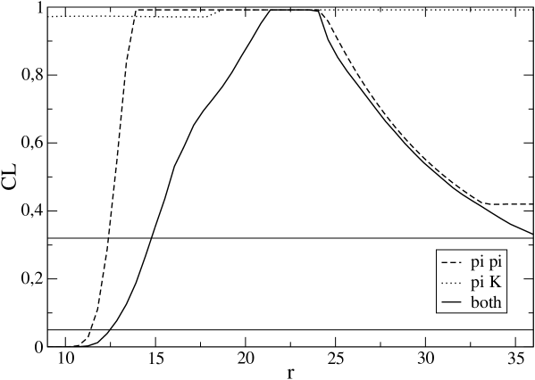
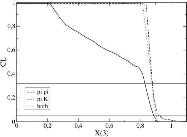
Figure 1: CL profiles for $r=m_{s}/m$ (top) and $X(3)=2m\Sigma(3)/(F_{\pi}^{2}M_{\pi}^{2})$ (bottom). The dashed line corresponds to experimental information on $\pi\pi$ scattering, the dotted line to $\pi K$ scattering, and the solid line to the combination of both sets. The two horizontal lines indicate the confidence intervals at 68 and 95% CL.

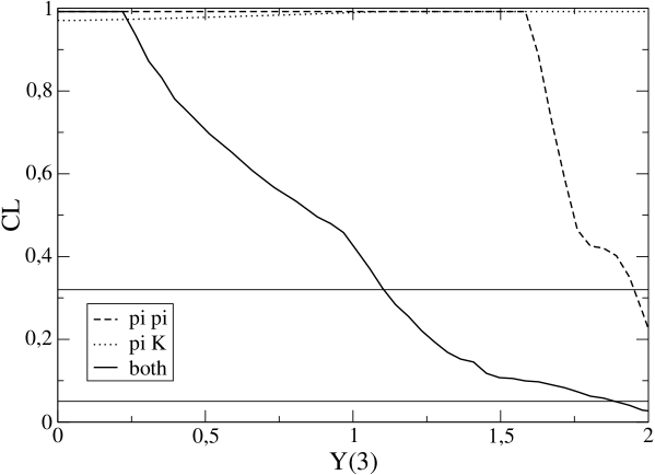
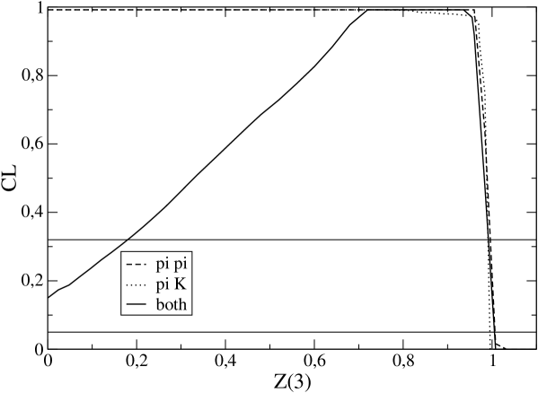
Figure 2: CL profiles for $Y(3)=2mB_{0}/M_{\pi}^{2}$ (top) and $Z(3)=F_{0}^{2}/F_{\pi}^{2}$ (bottom). The dashed line corresponds to experimental information on $\pi\pi$ scattering, the dotted line to $\pi K$ scattering, and the solid line to the combination of both sets. The two horizontal lines indicate the confidence intervals at 68 and 95% CL.

5.2 Comparison with some earlier works

5.2.1 $\pi\pi$ scattering

For $\pi\pi$ scattering, it is interesting to compare our results with ref. [12], which shares some ideas and issues with the present paper. This work differs on three points from ref. [12] : we include $\pi K$ scattering in our analysis, we choose as observables the scattering amplitudes in subthreshold regions rather than the subtraction constants involved in dispersive representations, we perform the statistical analysis in a frequentist framework rather than a Bayesian one.

We observe the same qualitative features in both analyses. As expected, low values of $r$ are strongly disfavoured. Indeed, the analysis of currently available data on $\pi\pi$ scattering [4] provides a value of $X(2)$, eq. (6). As illustrated in fig. 1 of ref. [1], $X(2)$ is related to $r$ through the pion and kaon mass and decay constant identities, eqs. (15)-(2.3): the value of $X(2)$ from ref. [4] favours the same range for the quark mass ratio as the upper plot in fig. 1. On the other hand, we find that $X(3)$ and $Z(3)$ are only constrained through an upper bound, in numerical agreement with the paramagnetic inequalities $X(3)\leq X(2)$ and $Z(3)\leq Z(2)$.

This agreement is particularly gratifying since the method of analysis of the present work does not require computing any $N_{f}=2$ chiral order parameters or related subtraction constants like refs. [4, 12]. Moreover, one can see an improvement compared to the latter references, thanks to the frequentist approach chosen here. In ref. [12], it was difficult to disentangle the effect of the data from that of the Bayesian priors inside a posterior p.d.f. : the so-called “reference profiles” (p.d.f.s from priors but no data) had to be compared to the posterior p.d.f.s (p.d.f.s from priors and data) to judge the impact of $\pi\pi$ data. In the present paper, this intricate procedure and the arbitrariness induced by Bayesian priors are avoided : it is clearly seen that $\pi\pi$ data constrains $X(3)$ and $Z(3)$ only through the values of $X(2)$ and $Z(2)$ and the corresponding paramagnetic upper bounds.

5.2.2 $\pi K$ scattering

For $\pi K$ scattering, we can compare our results with ref. [10], where the solutions of the Roy-Steiner dispersion relations were used to reconstruct the amplitudes in the subthreshold region. These amplitudes were expanded around the point $s=u$, $t=0$, and the coefficients of the polynomials, $C^{+}_{ij}$ and $C^{-}_{ij}$, were matched with their NLO chiral expansions in order to determine some $O(p^{4})$ LECs. This led to a determination of $L_{1},L_{2},L_{3}$ recalled in the previous section, and to a value of $L_{4}$ suggesting a significant suppression of $Z(3)$. The value of $L_{6}$, though affected by large uncertainties, indicated also a suppression of $X(3)$, stronger than that of $Z(3)$ :

$${\rm Ref.}~{}\cite[cite]{[\@@bibref{}{roypika}{}{}]}:L_{4}^{r}(M_{\rho})=(0.53\pm 0.39)\cdot 10^{-3}\,,\qquad[2L_{6}^{r}+L_{8}^{r}](M_{\rho})=(3.66\pm 1.52)\cdot 10^{-3}\,.$$ (71)

Using eq. (34) and the other results of sec. 3.1 in ref. [12], and taking $L_{8}^{r}(M_{\rho})=(0.9\pm 0.3)\cdot 10^{-3}$ [9] we can convert these results into the parameters of interest: following these results, $X(3)$ would stand between 0.15 and 0.41, $Z(3)$ between 0.14 and 0.92, and $Y(3)$ between 0.44 and 1.05. Obviously, the low values of $X(3)$ and $Z(3)$ indicate that the values obtained in ref. [10], relying on the assumption of small vacuum fluctuations and on $X(3)$ and $Z(3)$ close to 1, should be reassessed relaxing this hypothesis.

If our results for the combined $\pi\pi$ and $\pi K$ data point towards a similar pattern, our analysis of $\pi K$ data alone provides weaker constraints than that of ref. [10]. At least two different reasons lead us to weaker constraints. First, we have explicitly take into account the presence of NNLO contributions which were neglected in the $O(p^{4})$ analysis of ref. [10] and which may affect significantly the energy-dependent part of the amplitudes. Secondly, the analysis in ref. [10] assumes explicitly the smallness of vacuum fluctuations : once we drop this assumption, a smaller value of $L_{4}$ (and thus a value of $Z(3)$ close to 1) can be compensated by the variation of other parameters, such as the quark mass ratio $r$. These two phenomena may explain the weaker constraints observed in our analysis.

5.2.3 Combined analyses

For the combined analysis of $\pi\pi$ and $\pi K$ scatterings, we can compare our results with refs. [20, 21]. The authors took a different approach from ours, computing NNLO chiral expansions to $\pi\pi$ and $\pi K$ scattering amplitudes, and matching with results on $\pi\pi$ scattering (scattering lengths) and $\pi K$ scattering (scattering lengths and subthreshold expansion coefficients), supplemented with information on $K_{\ell 4}$ form factors. In agreement with the one-loop framework of ref. [9], these two-loop computations assume a numerical dominance of LO contributions and a quick convergence of $N_{f}=3$ chiral expansions.

In previous studies in this NNLO framework [22], the authors performed fits to pseudoscalar masses and decay constants [23], $K_{\ell 3}$ decays [24], and scalar form factors [19]. In each case, the values of the Zweig-rule suppressed $O(p^{4})$ LECs $L_{4}$ and $L_{6}$ had to be fixed by hand : fits of similarity quality could be obtained with values of these two constants corresponding either to small or large vacuum fluctuations of $s\bar{s}$ pairs. For scalar form factors, values of $L_{4}$ and $L_{6}$ larger than conventionally assumed led to an improvement in the convergence of observables (fits A,B,C compared to fit 10, in Table 2 of ref. [19]).

In the case of refs. [20, 21], the authors analysed $\pi\pi$ and $\pi K$ scattering amplitudes in the same NNLO framework. The fits were not able to reproduce some observables, in particular among $\pi K$ subthreshold coefficients. A particular subset of subthreshold coefficients and scattering lengths led to $L_{4}^{r}(M_{\rho})\simeq 0.2\cdot 10^{-3}$ and $L_{6}(M_{\rho})$ negative. Such values correspond to $F_{0}$ rather small compared to $F_{\pi}$, with a rather unsatisfying convergence of some observables : for instance, the pion mass exhibits instabilities in its chiral expansion [22]. It proves difficult to draw a fully consistent picture for the structure of QCD vacuum in the $N_{f}=3$ chiral limit from these results.

Some of the problems encountered in refs. [20, 21] were reassessed in ref. [30], in particular the determination of NNLO LECs. Following ref. [31], the many $O(p^{6})$ LECs are often estimated using resonance saturation. In ref. [30], the specific resonance Lagrangian used in refs. [20, 21] was shown to provide values for vector-dominated LECs rather far away from the expectations based on $\pi K$ dispersion relations, but other resonance Lagrangians failed also to reproduce these same results. Therefore, one may wonder whether the problems of convergence seen in [22] could stem from two different sources. The first one consists in the use of resonance saturation to fix $O(p^{6})$ counterterms, which is already delicate in vector channels and certainly questionable in the scalar sector. The second one is the observed slow convergence of chiral expansions, which contradicts the starting assumptions of the NNLO analysis. A comparison of Re$\chi$PT expansions with the NNLO formulae in refs. [20, 21] should highlight how large values of the $O(p^{4})$ LECs $L_{4}$ and $L_{6}$ might destabilise NNLO expansions and how the explicit resummation of vacuum fluctuations of our work echoes in the perturbative expansion adopted in the latter references.

5.2.4 Lattice

Other interesting developments are awaited from lattice simulations. The effects presented in this paper are related to strange sea-quarks, and can be tackled only with (2+1) dynamical fermions with light masses. Unfortunately, fermions with interesting chiral properties (Wilson, Ginsparg-Wilson, twisted-mass) [8] are still with at most two dynamical flavours. On the other hand, staggered fermions [33] have been exploited for simulations with (2+1) dynamical quarks, but their use is under much debate [34]. The presence of the fourth root of the fermion determinant yields non-localities which are not understood yet : at best, recovering QCD requires taking the various continuum limits in a very careful way.

A staggered version of chiral perturbation theory [35] has been developed to extract chiral LECs from the pseudoscalar spectrum. It attempts at reproducing the fourth-rooting of the fermion determinant and includes many other effects (lattice spacing, finite-volume effects, taste-breaking terms), leading to a number of LECs much larger than in continuum unstaggered $\chi$PT. The hope is that the LECs common to both theories should be identical because QCD ought to be recovered as a limit of lattice QCD with fourth-rooted staggered fermions. In practice [33], chiral fits to staggered data on the pseudoscalar spectrum must include a large number of parameters and thus are highly non-trivial. Mixed actions with domain-wall valence quarks and staggered sea quarks have also been considered to reduce the number of LECs involved in the associated chiral Lagrangian at the price of losing unitarity in addition to locality [36].

Bearing all these remarks in mind, we can focus on the following staggered values :

$${\rm Ref.}~{}\cite[cite]{[\@@bibref{}{MILC}{}{}]}:\quad r=27.2(4)\,,\quad[2L_{6}^{r}-L_{4}^{r}](M_{\eta})=0.5(1)(2)\cdot 10^{-3}\,,\quad L_{4}^{r}(M_{\eta})=0.1(2)(2)\cdot 10^{-3}\,.$$ (72)

Combining the errors in quadrature and using eq. (34) and the other results of sec. 3.1 in ref. [12], we can convert these results into the parameters of interest: following these lattice results, $X(3)$ would stand between 0.55 and 0.95, $Z(3)$ between 0.57 and 1.04, and $Y(3)$ between 0.67 and 1.08, values which are not in striking disagreement with our results. Obviously, if the values of $X(3)$ and $Z(3)$ are on the smaller end of these ranges, i.e., if $L_{6}$ and $L_{4}$ are in the upper end of the range in ref. [33], the assumption of small vacuum fluctuations is not correct, and the extraction of the LECs by the means of staggered $\chi$PT should be reassessed more carefully.

As an alternative to such tests, which rely strongly on the usual treatment of chiral series, we proposed a lattice test of the size of $s\bar{s}$ vacuum fluctuations based on Re$\chi$PT in ref. [37]. We considered simulations with (2+1) flavours, with a strange quark mass at its physical value, but two $u,d$ light quarks with identical masses $\tilde{m}$ larger than their physical values $m$ and smaller than $m_{s}$. The larger values of the $u,d$ masses enhanced the impact of the vacuum fluctuations encoded in $L_{4}$ and $L_{6}$ on observables such as the masses and decay constants of pions and kaons. This led to a difference in the curvatures of $F_{P}^{2}$ and $F_{P}^{2}M_{P}^{2}$ ($P=\pi,K$) as functions of $q=\tilde{m}/m_{s}$, depending on the size of $X(3)$ and $Z(3)$. The effect was less pronounced in the case of $M_{P}^{2}$, obtained as the ratio of the two former observables, leading to a fairly linear behaviour as a function of $q$.

We proposed in the same reference a test of the size of $X(3)$ on the lattice from the pion and kaon spectrum, by considering the dependence on $q$ of the ratios :

$$R_{\pi}=\frac{\tilde{F}_{\pi}^{2}\tilde{M}_{\pi}^{2}}{qF_{\pi}^{2}M_{\pi}^{2}}\qquad R_{K}=\frac{2\tilde{F}_{K}^{2}\tilde{M}_{K}^{2}}{(q+1)F_{K}^{2}M_{K}^{2}}$$ (73)

where $\tilde{F}_{\pi}^{2}$ and $\tilde{M}_{\pi}^{2}$ denote quantities computed on the lattice with $u,d$ quarks of mass $\tilde{m}$. We assessed the leading finite-volume effects to conclude that large volumes (of side around 2.5 fm) were required to tame these effects.

In any case, more dedicated studies on (2+1) fermions with different actions, lattice spacings and volumes will be required in order to draw definite conclusions from lattice simulations on the structure of $N_{f}=3$ chiral vacuum.

6 Conclusion

Vacuum fluctuations of $s\bar{s}$ pairs can induce significant differences in the pattern of chiral symmetry breaking between the two conceivable chiral limits: $N_{f}=2$ ($m_{u}=m_{d}=0$ but $m_{s}$ kept at its physical values) and $N_{f}=3$ ($m_{u}=m_{d}=m_{s}=0$). These fluctuations might lead to a paramagnetic suppression of the two main chiral order parameters in the $N_{f}=3$ chiral limit, the quark condensate and the pseudoscalar decay constant, compared to their $N_{f}=2$ counterparts [1, 11]. Then, we would observe a numerical competition between leading-order (LO) and next-to-leading order (NLO) contributions in chiral series, through the two $O(p^{4})$ LECs $L_{4}$ and $L_{6}$ related to the violation of the Zweig rule in the scalar sector.

In order to shed light on the size of these fluctuations, we developed and modified the framework sketched in ref. [12] : Resummed Chiral Perturbation Theory or Re$\chi$PT. We applied it to our current knowledge of low-energy $\pi\pi$ and $\pi K$ scatterings. First, we recalled and detailed our treatment of one-loop chiral series in the case of large vacuum fluctuations: only a subset of “good” observables is assumed to converge globally (so that NNLO contributions are much smaller than the sum of LO and NLO contributions), the chiral series must be treated in a particular way to derive bare expansions an resum the effects of vacuum fluctuations, while NNLO remainders are introduced to keep track of higher-order contributions. Then, in this resummed framework, called Re$\chi$PT, we determined the one-loop expansions for $\pi\pi$ and $\pi K$ scattering amplitudes. Relying on our current experimental knowledge, we exploited solutions of Roy and Roy-Steiner equations within dispersive representations to determine the values of the amplitudes in subthreshold (unphysical) regions where chiral expansions should converge.

The two representations of the scattering amplitudes were matched in a frequentist approach (inspired by Rfit [13]). The output of this analysis are marginal CL curves, providing an upper bound on the confidence level (CL) for the optimal set of theoretical parameters at fixed $T_{i}=t_{i}$: the CL value is the probability that a new series of measurements will agree with the most favourable set of theoretical parameters (at $T_{i}=t_{i}$) in a worse way than the experimental results actually used in the analysis [14].

Unfortunately, the marginal CL profiles do not provide sharp peaks and thus stringent constraints on theoretical parameters at a statistically significant level. However, our results point towards some favoured regions of parameter space, see figs. 1 and 2. If only $\pi\pi$ scattering is included, the results obtained in earlier works [12] are recovered : small values of $r$ are disfavoured, whereas $X(3)$ and $Z(3)$ are only constrained to remain below their $N_{f}=2$ counterpart due to paramagnetic inequalities eq. (5). $\pi K$ scattering alone does not constrain strongly the various theoretical parameters, apart from setting bounds on $X(3)$ and $Z(3)$. The combination of the two pieces of information proves more interesting : the CL profile for $r$ peaks around 23, low values of $X(3)$ are preferred, whereas the CL for $Z(3)$ exhibits a broad peak around 0.8.

From the CL curves obtained from the combined analysis of $\pi\pi$ and $\pi K$ scattering, we obtain the following confidence intervals at 68 % CL :

$$r\geq 14.8\,,\qquad X(3)\leq 0.83\,,\qquad Y(3)\leq 1.1\,,\qquad 0.18\leq Z(3)\leq 1\,.\qquad[68\%\ {\rm CL}]$$ (74)

corresponding to the regions of parameter space where the marginal CL profiles lie above 0.32 [14].

The pattern of the marginal CL profiles is consistent with the scenario of significant vacuum fluctuations of $s\bar{s}$ pairs. It reminds one of the interesting possibility that the decrease of order parameters from $N_{f}=2$ massless flavours to $N_{f}=3$ is steeper in the case of the pseudoscalar decay constant $F^{2}(N_{f})$ than for the quark condensate $\Sigma(N_{f})$.

The present analysis constitutes a first attempt to analyse data with a limited statistical significance, and it relies strongly on the experimental results gathered on $\pi\pi$ and $\pi K$ scatterings. For $\pi\pi$ scattering, new results are expected from the NA48 collaboration on $K_{\ell 4}$ decays [7] and on the cusp in $K\to 3\pi$ [38, 39]. For $\pi K$ scattering, we hope to obtain more precise information from $D_{\ell 4}$ decays [40, 41] and $\tau\to K\pi\nu_{\tau}$ decays [42, 43]. In addition, lattice studies could soon provide results for three light flavours with well-controlled actions in the chiral regime. These new high-accuracy data should shed some more light on the chiral structure of QCD vacuum, and in particular on its dependence on the number of massless flavours and the role played by the vacuum fluctuations of $s\bar{s}$ pairs.

Appendix A One-loop bare expansions of scattering amplitudes

A.1 $\pi\pi$ scattering amplitude

Following the prescription in sec. 2.2 we obtain, for instance from ref. [16] :

$$F_{\pi}^{4}A_{\pi\pi} = \frac{2}{3}mB_{0}F_{0}^{2}+F_{0}^{2}\left(s-\frac{4}{3}M_{\pi}^{2}\right)$$

$$+\mu_{\pi}F_{0}^{2}\left[-4\left(s-\frac{4}{3}M_{\pi}^{2}\right)-2B_{0}m\right]+\mu_{K}F_{0}^{2}\left[-2\left(s-\frac{4}{3}M_{\pi}^{2}\right)-\frac{4}{3}B_{0}m\right]$$

$$-\frac{2}{9}\mu_{\eta}F_{0}^{2}B_{0}m$$

$$+16B_{0}mL_{4}^{r}\left[\left(s-\frac{4}{3}M_{\pi}^{2}\right)(r+4)-\frac{4}{3}M_{\pi}^{2}\right]+32B_{0}mL_{5}^{r}\left(s-\frac{5}{3}M_{\pi}^{2}\right)$$

$$+\frac{64}{3}B_{0}^{2}m^{2}L_{6}^{r}(r+8)+\frac{256}{3}B_{0}^{2}m^{2}L_{8}^{r}$$

$$+4\left(2L_{1}^{r}+L_{3}^{r}\right)\left(s-2M_{\pi}^{2}\right)^{2}+4L_{2}^{r}\left[(t-2M_{\pi}^{2})^{2}+(u-2M_{\pi}^{2})^{2}\right]$$

$$+\frac{1}{2}\left[(s-2M_{\pi}^{2})^{2}+8B_{0}m(s-2M_{\pi}^{2})+12B_{0}^{2}m^{2}\right]J^{r}_{\pi\pi}(s)$$

$$+\frac{1}{4}\left[(t-2M_{\pi}^{2})^{2}J^{r}_{\pi\pi}(t)+(u-2M_{\pi}^{2})^{2}J^{r}_{\pi\pi}(u)\right]$$

$$+\frac{1}{8}\left[(s-2M_{\pi}^{2})^{2}+8B_{0}m(s-2M_{\pi}^{2})+16B_{0}^{2}m^{2}\right]J^{r}_{KK}(s)$$

$$+\frac{2}{9}B_{0}^{2}m^{2}J^{r}_{\eta\eta}(s)$$

$$+\frac{1}{2}\left[(s-u)t\left(2M^{r}_{\pi\pi}+M^{r}_{KK}\right)(t)+(s-t)u\left(2M^{r}_{\pi\pi}+M^{r}_{KK}\right)(u)\right]$$

where $\stackrel{{\scriptstyle\circ}}{{M}}_{P}^{2}$ denotes the leading-order pseudoscalar squared mass of the Goldstone boson $P$ and the tadpole logarithm is

$$\mu_{P}=\frac{\stackrel{{\scriptstyle\circ}}{{M}}_{P}^{2}}{32\pi^{2}F_{0}^{2}}\log\frac{M_{P}^{2}}{\mu^{2}}$$ (76)

We recast the amplitude in the following form

$$F_{\pi}^{4}A_{\pi\pi} = \mathcal{A}+\left(s-\frac{4}{3}M_{\pi}^{2}\right)\times\mathcal{B}$$

$$+4(2L_{1}^{r}+L_{3})(s-2M_{\pi}^{2})^{2}+4L_{2}^{r}[(t-2M_{\pi}^{2})^{2}+(u-2M_{\pi}^{2})^{2}]$$

$$+\frac{1}{2}[(s-2M_{\pi}^{2})^{2}+8mB_{0}(s-2M_{\pi}^{2})+12m^{2}B_{0}^{2}]J^{r}_{\pi\pi}(s)$$

$$+\frac{1}{4}[(t-2M_{\pi}^{2})^{2}J^{r}_{\pi\pi}(t)+(u-2M_{\pi}^{2})^{2}J^{r}_{\pi\pi}(u)]$$

$$+\frac{1}{8}[(s-2M_{\pi}^{2})^{2}+8mB_{0}(s-2M_{\pi}^{2})+16m^{2}B_{0}^{2}]J^{r}_{KK}(s)$$

$$+\frac{1}{18}4m^{2}B_{0}^{2}J^{r}_{\eta\eta}(s)$$

$$+\frac{1}{2}[(s-u)t\times(2M^{r}_{\pi\pi}+M^{r}_{KK})(t)+(s-t)u\times(2M^{r}_{\pi\pi}+M^{r}_{KK})(u)]$$

where $\mathcal{A}$ and $\mathcal{B}$ are scale-dependent combinations of LECs :

$$3\times{\mathcal{A}} = 2mB_{0}F_{0}^{2}+64m^{2}B_{0}^{2}[(r+8)L_{6}^{r}+4L_{8}^{r}]-32mB_{0}M_{\pi}^{2}[2L_{4}^{r}+L_{5}^{r}]$$

$$-\frac{1}{32\pi^{2}}4m^{2}B_{0}^{2}\left[3\log\frac{M_{\pi}^{2}}{\mu^{2}}+(r+1)\log\frac{M_{K}^{2}}{\mu^{2}}+\frac{1}{9}(2r+1)\log\frac{M_{\eta}^{2}}{\mu^{2}}\right]$$

$$\mathcal{B} = F_{0}^{2}+16mB_{0}[(r+4)L_{4}^{r}+2L_{5}^{r}]$$

$$-\frac{1}{32\pi^{2}}2mB_{0}\left[4\log\frac{M_{\pi}^{2}}{\mu^{2}}+(r+1)\log\frac{M_{K}^{2}}{\mu^{2}}\right]$$

which correspond to $F_{\pi}^{2}M_{\pi}^{2}\alpha^{r}_{\pi\pi}/3$ and $\mathcal{B}$ to $F_{\pi}^{2}\beta^{r}_{\pi\pi}$ respectively, as defined in ref. [16].

In the above expressions, we have replaced the bare masses by the physical masses in the (tadpole) logs and in the loop functions $J^{r}$ and $M^{r}$. One can check explicitly that there is no $\mu$ dependence in the above expression of the amplitude : for each polynomial in $s-2M_{\pi}^{2},t-2M_{\pi}^{2},u-2M_{\pi}^{2}$, the dependence of the LECs on the renormalisation scale $\mu$ cancels that of $J^{r}$ and $M^{r}$.

A.2 $\pi K$ scattering amplitude

We recall the expression obtained in ref. [26] for the $I=3/2$ amplitude:

$$F_{\pi}^{2}F_{K}^{2}F^{3/2}_{\pi K} = \frac{F_{0}^{2}}{6}\Bigg{[}2M_{\pi}^{2}+2M_{K}^{2}+\stackrel{{\scriptstyle\circ}}{{M}}_{\pi}^{2}+\stackrel{{\scriptstyle\circ}}{{M}}_{K}^{2}-3s$$

$$+\frac{\mu_{\pi}}{8}[66s-34M_{\pi}^{2}-54M_{K}^{2}-15\stackrel{{\scriptstyle\circ}}{{M}}_{\pi}^{2}-21\stackrel{{\scriptstyle\circ}}{{M}}_{K}^{2}]$$

$$+\frac{\mu_{K}}{4}[30s-22M_{\pi}^{2}-18M_{K}^{2}-11\stackrel{{\scriptstyle\circ}}{{M}}_{\pi}^{2}-9\stackrel{{\scriptstyle\circ}}{{M}}_{K}^{2}]$$

$$+\frac{\mu_{\eta}}{24}[54s-54M_{\pi}^{2}-18M_{K}^{2}-17\stackrel{{\scriptstyle\circ}}{{M}}_{\pi}^{2}-11\stackrel{{\scriptstyle\circ}}{{M}}_{K}^{2}]$$

$$+8L_{1}^{r}(t-2M_{\pi}^{2})(t-2M_{K}^{2})+4L_{2}^{r}[(s-M_{\pi}^{2}-M_{K}^{2})^{2}+(u-M_{\pi}^{2}-M_{K}^{2})^{2}]$$

$$+2L_{3}[(u-M_{\pi}^{2}-M_{K}^{2})^{2}+(t-2M_{\pi}^{2})(t-2M_{K}^{2})]$$

$$+8L_{4}^{r}[\stackrel{{\scriptstyle\circ}}{{M}}_{\pi}^{2}(t-\frac{1}{2}s+\frac{1}{3}M_{\pi}^{2}-\frac{5}{3}M_{K}^{2})+\stackrel{{\scriptstyle\circ}}{{M}}_{K}^{2}(t-s-\frac{4}{3}M_{\pi}^{2}+\frac{2}{3}M_{K}^{2})]$$

$$+\frac{4}{3}L_{5}^{r}[\stackrel{{\scriptstyle\circ}}{{M}}_{\pi}^{2}(2M_{\pi}^{2}-3s)+\stackrel{{\scriptstyle\circ}}{{M}}_{K}^{2}(2M_{K}^{2}-3s)]+\frac{8}{3}L_{6}^{r}[\stackrel{{\scriptstyle\circ}}{{M}}_{\pi}^{4}+15\stackrel{{\scriptstyle\circ}}{{M}}_{\pi}^{2}\stackrel{{\scriptstyle\circ}}{{M}}_{K}^{2}+2\stackrel{{\scriptstyle\circ}}{{M}}_{K}^{4}]$$

$$+\frac{8}{3}L_{8}^{r}[\stackrel{{\scriptstyle\circ}}{{M}}_{\pi}^{4}+6\stackrel{{\scriptstyle\circ}}{{M}}_{\pi}^{2}\stackrel{{\scriptstyle\circ}}{{M}}_{K}^{2}+\stackrel{{\scriptstyle\circ}}{{M}}_{K}^{4}]$$

$$+\frac{t}{2}(u-s)[M^{r}_{\pi\pi}(t)+\frac{1}{2}M^{r}_{KK}(t)]$$

$$+\frac{3}{8}\{(s-t)[L_{\pi K}(u)-uM^{r}_{\pi K}(u)]+(M_{K}^{2}-M_{\pi}^{2})^{2}M^{r}_{\pi K}(u)\}$$

$$+\frac{3}{8}\{(s-t)[L_{K\eta}(u)-uM^{r}_{K\eta}(u)]+(M_{K}^{2}-M_{\pi}^{2})^{2}M^{r}_{K\eta}(u)\}$$

$$+\frac{1}{8}(M_{K}^{2}-M_{\pi}^{2})K_{\pi K}(u)[5(u-M_{\pi}^{2}-M_{K}^{2})+3\stackrel{{\scriptstyle\circ}}{{M}}_{\pi}^{2}+3\stackrel{{\scriptstyle\circ}}{{M}}_{K}^{2}]$$

$$+\frac{1}{8}(M_{K}^{2}-M_{\pi}^{2})K_{K\eta}(u)[3(u-M_{\pi}^{2}-M_{K}^{2})+\stackrel{{\scriptstyle\circ}}{{M}}_{\pi}^{2}+\stackrel{{\scriptstyle\circ}}{{M}}_{K}^{2}]$$

$$+\frac{1}{4}J^{r}_{\pi K}(s)(s-M_{\pi}^{2}-M_{K}^{2})^{2}$$

$$+\frac{1}{32}J^{r}_{\pi K}(u)[11(u-M_{\pi}^{2}-M_{K}^{2})^{2}+10(u-M_{\pi}^{2}-M_{K}^{2})(\stackrel{{\scriptstyle\circ}}{{M}}_{\pi}^{2}+\stackrel{{\scriptstyle\circ}}{{M}}_{K}^{2})+3(\stackrel{{\scriptstyle\circ}}{{M}}_{\pi}^{2}+\stackrel{{\scriptstyle\circ}}{{M}}_{K}^{2})^{2}]$$

$$+\frac{1}{32}J^{r}_{K\eta}(u)[u-M_{\pi}^{2}-M_{K}^{2}+\frac{1}{3}(\stackrel{{\scriptstyle\circ}}{{M}}_{\pi}^{2}+\stackrel{{\scriptstyle\circ}}{{M}}_{K}^{2})]^{2}$$

$$+\frac{1}{8}J^{r}_{\pi\pi}(t)[4M_{\pi}^{2}-2t-3\stackrel{{\scriptstyle\circ}}{{M}}_{\pi}^{2}][2M_{K}^{2}-t-2\stackrel{{\scriptstyle\circ}}{{M}}_{K}^{2}]$$

$$+\frac{3}{16}J^{r}_{KK}(t)[2M_{\pi}^{2}-t-2\stackrel{{\scriptstyle\circ}}{{M}}_{\pi}^{2}][2M_{K}^{2}-t-2\stackrel{{\scriptstyle\circ}}{{M}}_{K}^{2}]$$

$$+\frac{1}{8}J^{r}_{\eta\eta}(t)\stackrel{{\scriptstyle\circ}}{{M}}_{\pi}^{2}[t-2M_{K}^{2}+\frac{10}{9}\stackrel{{\scriptstyle\circ}}{{M}}_{K}^{2}]$$

This expression is renormalisation-scale independent. In both $\pi\pi$ and $\pi K$ scatterings, the one-loop expressions obtained with the usual treatment of three-flavour $\chi$PT [9] are recovered if we treat chiral series perturbatively and neglect the (potentially large) difference between the truncated $O(p^{2})$ expressions and the physical values of the pseudoscalar masses and decay constants.

Appendix B Computation of the amplitudes

The amplitudes are smooth functions of the various experimental inputs. This means in particular that there will be significant correlations among the value of the same scattering amplitude at different points in the Mandelstam plane. We compute these correlations according to the following procedure. Let us call $a_{k}$ ($k=1\ldots n$) the parameters describing the variations of the experimental inputs. To each of these parameters is attached an uncertainty ($\sigma_{k}$), and the correlations among them are encoded in a covariance matrix $D_{kl}$, or equivalently, a reduced covariance matrix $H_{kl}=D_{kl}/(\sigma_{k}\sigma_{l})$. We compute the mean value $m_{i}$ of the observables $x_{i}$’s by setting all the parameters $a_{k}$ to their central value $\bar{a}_{k}$: $m_{i}\equiv x_{i}(\bar{a}_{k})$. Then, we vary the parameters one by one (the others being kept at their central value) and compute each time:

$$\Delta^{k}_{i}\equiv x_{i}\!\!\left(\bar{a}_{k}+\frac{\sigma_{k}}{\rho}\right)-m_{i}=\frac{\sigma_{k}}{\rho}\times\frac{\partial x_{i}}{\partial a_{k}}+\ldots$$ (81)

where $\rho$ is a largish parameter (around 10), and the ellipsis denotes higher derivatives. Once this is done for all the parameters, we compute the covariance matrix for the observables:

$$V_{ij}\equiv\rho^{2}\sum_{kl}\Delta^{k}_{i}\Delta^{l}_{j}H_{kl}=\sum_{kl}\frac{\partial x_{i}}{\partial a_{k}}\frac{\partial x_{j}}{\partial a_{l}}D_{kl}+\ldots$$ (82)

The same procedure was followed in ref. [10] to determine the correlation matrix between the two $\pi K$-scattering lengths.

For the $\pi\pi$ scattering amplitude, we obtain the following values and errors for the amplitude at the limits of the subthreshold region $(s,t,u)$

$$(2M_{\pi}^{2},M_{\pi}^{2},M_{\pi}^{2}) A=2.84\pm 0.16$$ (83)

$$(M_{\pi}^{2}/2,3/2M_{\pi}^{2},3/2M_{\pi}^{2}) A=-1.03\pm 0.12$$ (84)

$$(M_{\pi}^{2}/2,3M_{\pi}^{2},M_{\pi}^{2}/2) A=-1.08\pm 0.11$$ (85)

For $\pi K$ scattering, we have in a similar way

$$(M_{K}^{2},2M_{\pi}^{2},M_{K}^{2}) B=4.09\pm 0.64\qquad C=0$$ (86)

$$(M_{K}^{2},0,M_{K}^{2}+2M_{\pi}^{2}) B=2.96\pm 0.60\qquad C=-0.95\pm 0.03$$ (87)

$$(M_{K}^{2}+M_{\pi}^{2},0,M_{K}^{2}+M_{\pi}^{2}) B=2.61\pm 0.60\qquad C=0$$ (88)

The zeroes of $C$ are due to its antisymmetry under $s-u$ exchange. Uncertainties are correlated.

Appendix C Treatment of correlated data

We expect strong correlations among the data points. This is reflected by the fact that the matrix $C$ is nearly degenerate, and therefore cannot be inverted easily. In order to treat this problem, one can diagonalize  the matrix $C$:

$$C=UDU^{T}\,,\qquad D={\rm diag}(\lambda_{1},\ldots,\lambda_{n})\,,\qquad UU^{T}=U^{T}U=1\,,$$ (89)

which yields the corresponding likelihood:

$${\mathcal{L}}(\Delta V) = \exp\left[-\frac{1}{2}\Delta V^{T}\ C^{-1}\ \Delta V\right]/\sqrt{\det(2\pi C)}$$ (90)

$$= \exp\left[-\frac{1}{2}\Delta V^{T}\ UD^{-1}U^{T}\ \Delta V\right]/\sqrt{\det(2\pi C)}\,.$$ (91)

Let us split the set of eigenvalues in two categories: large eigenvalues of order 1, collected in the diagonal matrix $\tilde{D}$, and almost vanishing eigenvalues, smaller than a cut-off and gathered in the diagonal matrix $D_{0}$:

$$D=\tilde{D}+D_{0}\,,\qquad\tilde{C}=U\tilde{D}U^{T}\,,\qquad C_{0}=UD_{0}U^{T}\,.$$ (92)

The eigenvalues in $D_{0}$ are responsible for the near degeneracy of the matrix. In the corresponding directions, the exponential could be approximated with a Dirac distribution and would yield constrains on NNLO and higher-order remainders. Our approximation by a low-degree polynomial is expected to hold at the level of a few percent: numerically, a perfect agreement between data and experiment occurs already if $\Delta V=O(1\%)$. Therefore, we cannot make much use of eigenvalues of the covariance matrix much smaller than $(1\%)^{2}=10^{-4}$. This leads us to limit the analysis to the subspace where $\tilde{D}$ is non-vanishing, and to define on this subspace $D^{-1}\equiv\tilde{D}^{-1}$ (see Ch. 2.6 in ref. [44] for a more detailed discussion on the relationships between singular value decomposition and matrix inversion). We chose to set the limit between small and large eigenvalues of order $10^{-8}$ (with only a very mild dependence of our results on the exact value of the cutoff).

Appendix D Impact of combining $\pi\pi$ and $\pi K$ data for marginal CL profiles

As shown in sec. 5.1, the analysis of $\pi\pi$ data in our framework puts a lower bound on $r$ ($r\geq 12$ at 68 % CL), and an upper bound on $X(3)$ and $Z(3)$ (below 0.85 and 0.95 respectively). $\pi K$ scattering does seem to bring only a lower bound on $X(3)$. The combination of these two pieces of information proves much more powerful and allows one to extract CL intervals on $r$, $X(3)$, $Y(3)$ and $Z(3)$. Indeed, we recall that our statistical method, inspired by the Rfit approach [13], consists in the following steps : determine the absolute minimum of $\chi^{2}$ first, then fix a particular theoretical parameter $a$ (among $r$, $X(3)$, $Y(3)$, $Z(3)$) and compute the corresponding relative minimum of $\chi^{2}$, finally extract a CL (actually a $P$-value [14] from the difference between the two values of $\chi^{2}$. This amounts to computing

$${\rm CL}[a|{\rm data}]={\rm Max}_{\mu}{\rm CL}[a;\mu|{\rm data}]$$ (93)

where $\mu$ collects all the remaining theoretical parameters (including $L_{i}$ and NNLO remainders). Therefore, the CL profiles obtained in our approach correspond to upper bounds on the CLs. In particular, it is enough that one set of theoretical parameters $\mu$ yields the same value of $\chi^{2}$ as the absolute minimum to get ${\rm CL}(a)=1$.

We have many theoretical parameters for the description of the scattering amplitudes : in addition to $r$, $X(3)$ and $Z(3)$, we have the $O(p^{4})$ LECs $L_{1,2,3}$ and (direct and indirect) NNLO remainders. Therefore, it is not particularly surprising that either $\pi\pi$ or $\pi K$ scattering alone is not enough to simultaneously put constrains on all these parameters : many equivalent situations (with identical $\chi^{2}$ and thus ${\rm CL}$) can be obtained with different sets of theoretical parameters. This degeneracy, in particular for the minimum $\chi^{2}$, comes from the possibility of compensating a variation in $a$ by a modification of the remaining theoretical parameters $\mu$ within the allowed ranges, which tends to yield flat CL profiles when we consider only one amplitude.

This underdetermination of the theoretical parameters – and the resulting degeneracy in CL values – is lifted once several sets of different sources are considered. In the present case, $\pi\pi$ data puts constraints on the quark mass ratio $r$ and on some of the $O(p^{4})$ derivative couplings. Because of these constraints, the regions of theoretical parameters with identical CLs are reduced, and thus the CL curves associated with $\pi K$ scattering exhibit more distinctive features.

As an illustration of this phenomenon, we compute the CL for $\pi K$ data alone with $L_{1},L_{2},L_{3}$ and $r$ fixed to specific values, in order to mimic the interplay between $\pi\pi$ and $\pi K$ data in CL curves. Let us set $L_{1},L_{2},L_{3}$ to the values corresponding to the absolute minimum of the $\chi^{2}$ when both $\pi\pi$ and $\pi K$ data are considered

$$L_{1}^{r}(M_{\rho})=-0.31\cdot 10^{-3}\,,\qquad L_{2}^{r}(M_{\rho})=2.12\cdot 10^{-3}\,,\qquad L_{3}^{r}(M_{\rho})=-0.64\cdot 10^{-3}\,,$$ (94)

and let us set $r$ to four different values $r=10,20,30,35$. With these theoretical parameters fixed, we determine ${\rm CL}[X(3);r,L_{1,2,3}|\pi K]$ and ${\rm CL}[Z(3);r,L_{1,2,3}|\pi K]$ profiles, which are drawn in fig. 3. We can see that the CL profiles of $X(3)$ and $Z(3)$ for $r=20$ are very similar to the solid lines shown in figs. 1 and 2, corresponding to $CL[X(3)|\pi\pi,\pi K]$ and $CL[Z(3)|\pi\pi,\pi K]$. On the other hand, the curves for $r=10,30,35$ are somewhat broader and flatter.

The CL curves obtained for $\pi K$ scattering in figs. 1 and 2 are ${\rm CL}[X(3)|\pi K]$ and ${\rm CL}[Z(3)|\pi K]$, which correspond to the envelope of all the CL profiles of the form ${\rm CL}[X(3);r,L_{1,2,3}|\pi K]$ and ${\rm CL}[Z(3);r,L_{1,2,3}|\pi K]$ when varying $r$ (and $L_{1,2,3}$). This superimposition, dominated by values of $r$ around 35, eventually yields the flat profiles in $X(3)$ and $Z(3)$ observed in figs. 1 and 2. On the other hand, when we combine $\pi\pi$ and $\pi K$ scatterings, a value of $r$ around 20 is preferred by $\pi\pi$ data (together with some ranges for $L_{1,2,3}$). Therefore, the contribution from $\pi K$ scattering to ${\rm CL}[X(3)|\pi\pi,\pi K]$ and ${\rm CL}[Z(3)|\pi\pi,\pi K]$ is close to the CL curve obtained for ${\rm CL}[X(3);r=20,L_{1,2,3}|\pi K]$ and ${\rm CL}[Z(3);r=20,L_{1,2,3}|\pi K]$, i.e. $r=20$ in fig. 3. This phenomenon explains how the information on theoretical parameters can be hidden in $\pi K$ scattering, but is unveiled once combined with $\pi\pi$ scattering, lifting the degeneracy in the CLs and leading to a sharper determination of $X(3)$ and $Z(3)$.

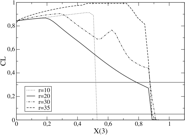
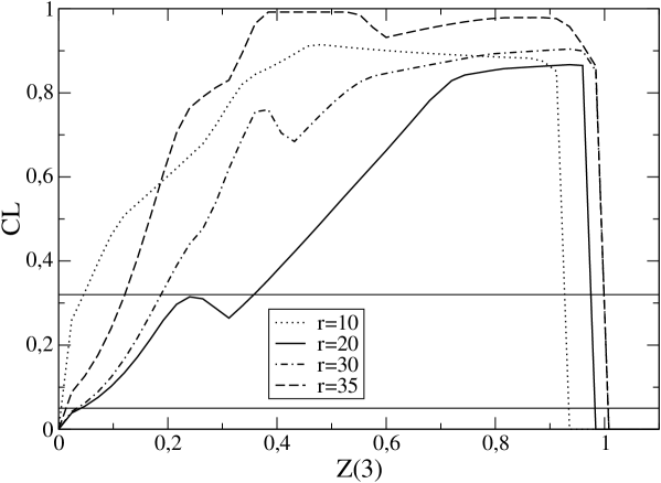
Figure 3: CL profiles for $X(3)=2m\Sigma(3)/(F_{\pi}^{2}M_{\pi}^{2}$ (top) and $Z(3)=F_{0}^{2}/F_{\pi}^{2}$ (bottom), obtained from the combination of the experimental information on $\pi\pi$ and $\pi K$ scatterings, with $L_{1},L_{2},L_{3}$ set to the values minimizing the complete $\chi^{2}$ (see text). The three curves corresponding to four different (imposed) values of $r=10,20,30,35$. The two horizontal lines indicate the confidence intervals at 68 and 95% CL.

References

- [1] S. Descotes-Genon, L. Girlanda and J. Stern, JHEP 0001, 041 (2000) [hep-ph/9910537].
- [2] S. Pislak et al. [BNL-E865 Collaboration], Phys. Rev. Lett. 87 (2001) 221801 [hep-ex/0106071]; Phys. Rev. D 67 (2003) 072004 [hep-ex/0301040].
- [3] B. Ananthanarayan, G. Colangelo, J. Gasser and H. Leutwyler, Phys. Rept. 353 (2001) 207 [hep-ph/0005297].
- [4] S. Descotes-Genon, N. H. Fuchs, L. Girlanda and J. Stern, Eur. Phys. J. C 24, 469 (2002) [hep-ph/0112088].
- [5] G. Colangelo, J. Gasser and H. Leutwyler, Phys. Rev. Lett. 86 (2001) 5008 [hep-ph/0103063].
- [6] J. Gasser and H. Leutwyler, Annals Phys. 158, 142 (1984).
- [7] L. Masetti [NA48 collaboration], Talk at the 33rd International Conference on High Energy Physics (ICHEP 06), hep-ex/0610071.
- [8] L. Del Debbio, L. Giusti, M. Luscher, R. Petronzio and N. Tantalo, hep-lat/0610059, hep-lat/0701009. D. Becirevic, Ph. Boucaud, V. Lubicz, G. Martinelli, F. Mescia, S. Simula and C. Tarantino, Phys. Rev. D 74, 034501 (2006) [hep-lat/0605006]. Ph. Boucaud et al. [ETM Collaboration], hep-lat/0701012.
- [9] J. Gasser and H. Leutwyler, Nucl. Phys. B 250, 465 (1985).
- [10] P. Büttiker, S. Descotes-Genon and B. Moussallam, Eur. Phys. J. C 33, 409 (2004) [hep-ph/0310283].
- [11] S. Descotes-Genon, L. Girlanda and J. Stern, Eur. Phys. J. C 27, 115 (2003) [hep-ph/0207337].
- [12] S. Descotes-Genon, N. H. Fuchs, L. Girlanda and J. Stern, Eur. Phys. J. C 34, 201 (2004) [hep-ph/0311120].
- [13] A. Hocker, H. Lacker, S. Laplace and F. Le Diberder, Eur. Phys. J. C 21 (2001) 225 [hep-ph/0104062].
-
[14]
W.J. Metzger, Statistical Methods in Data Analysis,
http://www.hef.kun.nl/ wes/stat_course/statist.pdf F. James, Statistical Methods in experimental physics, World Scientific 2006. - [15] N. H. Fuchs, H. Sazdjian and J. Stern, Phys. Lett. B 238 (1990) 380, Phys. Lett. B 269 (1991) 183, Phys. Rev. D 47 (1993) 3814 [hep-ph/9301244].
- [16] M. Knecht, B. Moussallam, J. Stern and N. H. Fuchs, Nucl. Phys. B 457, 513 (1995) [hep-ph/9507319].
- [17] B. Moussallam, Eur. Phys. J. C 14, 111 (2000) [hep-ph/9909292] ; JHEP 0008, 005 (2000) [hep-ph/0005245].
- [18] S. Descotes-Genon, JHEP 0103, 002 (2001) [hep-ph/0012221].
- [19] J. Bijnens and P. Dhonte, JHEP 0310, 061 (2003) [hep-ph/0307044].
- [20] J. Bijnens, P. Dhonte and P. Talavera, JHEP 0401, 050 (2004) [hep-ph/0401039].
- [21] J. Bijnens, P. Dhonte and P. Talavera, JHEP 0405, 036 (2004) [hep-ph/0404150].
- [22] J. Bijnens, Prog. Part. Nucl. Phys. 58 (2007) 521 [hep-ph/0604043].
- [23] G. Amoros, J. Bijnens and P. Talavera, Nucl. Phys. B 568 (2000) 319 [hep-ph/9907264]; Nucl. Phys. B 602 (2001) 87 [hep-ph/0101127].
- [24] J. Bijnens and P. Talavera, Nucl. Phys. B 669 (2003) 341 [hep-ph/0303103].
- [25] S. Descotes-Genon and J. Stern, Phys. Lett. B 488, 274 (2000) [hep-ph/0007082].
- [26] V. Bernard, N. Kaiser and U. G. Meissner, Phys. Rev. D 43 (1991) 2757.
- [27] A. Manohar and H. Georgi, Nucl. Phys. B 234 (1984) 189. H. Georgi, Phys. Lett. B 298 (1993) 187 [hep-ph/9207278].
- [28] J. Charles et al. [CKMfitter Group], Eur. Phys. J. C 41 (2005) 1 [hep-ph/0406184].
- [29] J. Stern, hep-ph/9801282. S. Descotes-Genon and J. Stern, Phys. Rev. D 62, 054011 (2000) [hep-ph/9912234].
- [30] K. Kampf and B. Moussallam, Eur. Phys. J. C 47 (2006) 723 [hep-ph/0604125].
- [31] G. Ecker, J. Gasser, A. Pich and E. de Rafael, Nucl. Phys. B 321 (1989) 311.
- [32] G. Amoros, J. Bijnens and P. Talavera, Phys. Lett. B 480 (2000) 71 [hep-ph/9912398], Nucl. Phys. B 585 (2000) 293 [Erratum-ibid. B 598 (2001) 665] [hep-ph/0003258].
- [33] C. Bernard et al. [MILC Collaboration], hep-lat/0609053.
- [34] M. Creutz, hep-lat/0603020, hep-lat/0701018. C. Bernard, M. Golterman, Y. Shamir and S. R. Sharpe, hep-lat/0603027. S. Durr, PoS LAT2005 (2006) 021 [hep-lat/0509026]. S. R. Sharpe, PoS LAT2006 (2006) 022 [hep-lat/0610094].
- [35] S. R. Sharpe and R. S. Van de Water, Phys. Rev. D 71 (2005) 114505 [hep-lat/0409018].
- [36] J. W. Chen, D. O’Connell, R. S. Van de Water and A. Walker-Loud, Phys. Rev. D 73 (2006) 074510 [hep-lat/0510024]. D. O’Connell, hep-lat/0609046. J. W. Chen, D. O’Connell and A. Walker-Loud, Phys. Rev. D 75 (2007) 054501 [hep-lat/0611003].
- [37] S. Descotes-Genon, Eur. Phys. J. C 40 (2005) 81 [hep-ph/0410233].
- [38] J. R. Batley et al. [NA48/2 Collaboration], Phys. Lett. B 633 (2006) 173 [hep-ex/0511056].
- [39] N. Cabibbo, Phys. Rev. Lett. 93 (2004) 121801 [hep-ph/0405001]. N. Cabibbo and G. Isidori, JHEP 0503 (2005) 021 [hep-ph/0502130]. G. Colangelo, J. Gasser, B. Kubis and A. Rusetsky, Phys. Lett. B 638 (2006) 187 [hep-ph/0604084]. E. Gamiz, J. Prades and I. Scimemi, Eur. Phys. J. C 50 (2007) 405 [hep-ph/0602023].
- [40] J. M. Link et al. [FOCUS Collaboration], Phys. Lett. B 607 (2005) 67 [hep-ex/0410067]. M. R. Shepherd et al. [CLEO Collaboration], Phys. Rev. D 74, 052001 (2006) [hep-ex/0606010].
- [41] C. L. Y. Lee, M. Lu and M. B. Wise, Phys. Rev. D 46, 5040 (1992). B. Ananthanarayan and K. Shivaraj, Phys. Lett. B 628 (2005) 223 [hep-ph/0508116].
- [42] R. Barate et al. [ALEPH Collaboration], Eur. Phys. J. C 11 (1999) 599 [hep-ex/9903015]. G. Abbiendi et al. [OPAL Collaboration], Eur. Phys. J. C 35 (2004) 437 [hep-ex/0406007].
- [43] M. Jamin, A. Pich and J. Portoles, Phys. Lett. B 640, 176 (2006) [hep-ph/0605096]. M. Jamin, J. A. Oller and A. Pich, Phys. Rev. D 74, 074009 (2006) [hep-ph/0605095].
- [44] W.H. Press, S.A. Teukolsky, W.T. Vetterling, B.P. Flannery, Numerical recipes - The art of scientific computing, Cambridge University Press.