The Sivers single-spin asymmetry in photon-jet production

Abstract

We study a weighted asymmetry in the azimuthal distribution of photon-jet pairs produced in the process $p^{\uparrow}p\to\gamma$ jet $X$ with a transversely polarized proton. We focus on the contribution of the Sivers effect only, considering experimental configurations accessible at RHIC-BNL. We show that predictions for the asymmetry, obtained in terms of gluonic-pole cross sections calculable in perturbative QCD, can be tested and clearly discriminated from those based on a generalized parton model, involving standard partonic cross sections. Experimental measurements of the asymmetry will therefore test our present understanding of single-spin asymmetries.

Single-spin asymmetries (SSA), particularly in processes with transversely polarized targets, have been measured in proton-proton collisions $p^{\uparrow}p\to\pi X$ (see, e.g., Adams et al. (1991)) and semi-inclusive deep inelastic scattering (SIDIS), $\ell p^{\uparrow}\to\ell^{\prime}\pi X$ Airapetian et al. (2005). Different theoretical approaches have been adopted to interpret these asymmetries and make predictions for other processes. In this paper, we make a clear-cut prediction for a simple process using the color-gauge-invariant QCD formalism (see, e.g., Qiu and Sterman (1999); Bacchetta et al. (2005); Kouvaris et al. (2006)) and compare it with the frequently used generalized parton model (see, e.g., Anselmino et al. (2006)).

In general, nonvanishing SSA require the interference between scattering amplitudes with different phases. Possible sources of phase shifts are initial- or final-state color interactions Brodsky et al. (2002). When describing high-energy processes, these color interactions can be included in parton distribution functions (PDFs). In standard gauges, they can be identified with the Wilson lines required to make the PDFs gauge invariant (see, e.g., Ji and Yuan (2002)).

The form of the Wilson line is fixed by the hard part of the scattering process and thus process-dependent. For instance, in SIDIS the Wilson line is future-pointing (it arises from gluon interactions with the outgoing quark), while in the Drell-Yan (DY) process ($pp^{\uparrow}\to l\bar{l}X$) the Wilson line is past-pointing (it arises from gluon interactions with the incoming antiquark) Collins (2002). This has a striking consequence for single-spin asymmetries. In the color-gauge-invariant approach, the asymmetries in DY have exactly the opposite sign compared to the generalized parton model expectation. This sign difference is a fundamental QCD prediction and its experimental verification would be crucial to confirm the validity of our present conceptual framework for analyzing hard hadronic reactions Efremov et al. (2005); Bomhof et al. (2007).

When considering a process different from SIDIS and DY, for instance $p^{\uparrow}p\to$ hadrons, the Wilson line structure becomes more intricate Bomhof et al. (2004). First of all, several partonic QCD processes contribute; secondly, each process has colored partons both in the initial and the final state, resulting in a competing effect of future- and past-pointing Wilson lines. It is therefore more challenging to derive clear-cut predictions for the sign of the SSA in these processes Bomhof et al. (2007).

In this letter we shall consider hadronic production of a photon and a jet in opposite hemispheres. This is the simplest case to test the formalism in processes with QCD hard scattering. After describing the kinematics of the process, we define a suitable weighted azimuthal asymmetry that contains the Sivers function Sivers (1990). We then present quantitative studies in a specific kinematical region and predict the sign of the asymmetry, which turns out to be opposite to the generalized parton model expectation, based on SIDIS results. The experimental confirmation of this prediction has the same significance as measuring the relative sign difference of the Sivers effect in SIDIS and the Drell-Yan process, and has the advantage that the cross-section for photon production is larger than for Drell-Yan.

The process under consideration is (see also Vogelsang and Yuan (2005))

$$p^{\uparrow}(P_{1})+p(P_{2})\to\gamma(K_{\gamma})+{\rm jet}(K_{j})+X.$$ (1)

This process is similar to $p^{\uparrow}p\to{\rm jet}\,{\rm jet}\,X$ studied in Boer and Vogelsang (2004); Bacchetta et al. (2005); Bomhof et al. (2007), to polarized DY (see, e.g., Boer (1999)), and to $p^{\uparrow}p\to\gamma\,X$ (see, e.g., Schmidt et al. (2005)). We fix the $z$ direction along $\bm{P}_{1}$ in the center-of-mass frame (c.m.). We use the pseudorapidities $\eta_{i}=-\ln\tan(\theta_{i}/2)$, where $\theta_{i}$ is the c.m. polar angle of the outgoing photon or jet. The components of the outgoing momenta perpendicular to $\bm{P}_{1}$ are denoted as $\bm{K}_{i\perp}$. We introduce the variables $x_{i\perp}=2|\bm{K}_{i\perp}|/\sqrt{s}$ and the azimuthal angles (see Fig. 1) Bacchetta et al. (2004)

$$\begin{split}\cos\phi_{i}&=\frac{(\hat{\bm{P}}_{1}\times{\bm{S}})}{|\hat{\bm{P}}_{1}\times{\bm{S}}|}\cdot\frac{(\hat{\bm{P}}_{1}\times{\bm{K}}_{i})}{|\hat{\bm{P}}_{1}\times{\bm{K}}_{i}|},\\ \sin\phi_{i}&=\frac{(\hat{\bm{P}}_{1}\times{\bm{S}})\cdot{\bm{K}}_{i}}{|\hat{\bm{P}}_{1}\times{\bm{S}}|\,|\hat{\bm{P}}_{1}\times{\bm{K}}_{i}|},\end{split}$$ (2)

with $\hat{\bm{P}}_{1}={\bm{P}}_{1}/|{\bm{P}}_{1}|$, where all vectors refer to the c.m. (or to any frame connected to the c.m. by a boost along $\hat{\bm{P}}_{1}$). Finally, we introduce the vector $r_{\perp}=K_{\gamma\perp}+K_{j\perp},$ and the angle $\delta\phi=\phi_{j}-\phi_{\gamma}-\pi$.

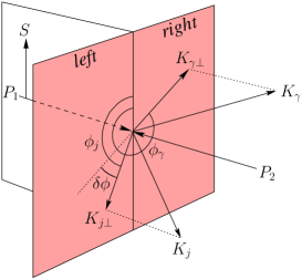
Figure 1: Azimuthal angles involved in the process. The vectors $K_{\gamma\perp}$, $K_{j\perp}$ lie on the plane perpendicular to $P_{1}$.

We focus our attention on the case in which $|\bm{r}_{\perp}|\ll|\bm{K}_{\gamma\perp}-\bm{K}_{j\perp}|$, i.e., when the photon and the jet are approximately back-to-back in the transverse plane. We retain only leading-order contributions in an expansion in $|\bm{r}_{\perp}|/|\bm{K}_{\gamma\perp}|$. In particular, this implies that $x_{\gamma\perp}=x_{j\perp}\equiv x_{\perp}$. For comparison’s sake, we will consistently make the same approximation in the generalized parton model Anselmino et al. (2006).

We now consider the following azimuthal moment Bacchetta et al. (2005)

$$M_{N}^{\gamma j}(\eta_{\gamma},\eta_{j},x_{\perp})=$$ (3)

$$\frac{\int\!d\phi_{j}\,d\phi_{\gamma}\frac{2|\bm{K}_{\gamma\perp}|}{M}\sin(\delta\phi)\cos(\phi_{\gamma})\,\frac{d\sigma}{d\phi_{j}\,d\phi_{\gamma}}}{\int\!d\phi_{j}\,d\phi_{\gamma}\,\frac{d\sigma}{d\phi_{j}\,d\phi_{\gamma}}}\equiv-\frac{A+B}{C}.$$

We expect the above integral to be dominated by the small-$\delta\phi$ region. Note that a positive value for this moment means that the sum of the photon and jet transverse momenta, $\bm{r}_{\perp}$, has a preference to lie on the right side of the transverse plane (as defined in Fig. 1), i.e., the photon–jet pair has a preference to go to the right.

Figure 2: Cut diagrams for $qg{\to}\gamma q$ scattering.

Figure 3: Cut diagrams for $q\bar{q}{\to}\gamma g$ scattering.

In terms of PDFs and partonic hard cross sections, the denominator of the above moment can be interpreted as

$$\begin{split}C&=x_{\perp}x_{1}x_{2}\,\textstyle{\sum_{q}}\Bigl{[}f_{1}^{g}(x_{1})\,f_{1}^{q}(x_{2})\,d\hat{\sigma}_{gq{\scriptscriptstyle\to}\gamma q}+f_{1}^{q}(x_{1})\\ &\quad\times\Bigl{(}f_{1}^{\bar{q}}(x_{2})\,d\hat{\sigma}_{q\bar{q}{\scriptscriptstyle\to}\gamma g}+f_{1}^{g}(x_{2})\,d\hat{\sigma}_{qg{\scriptscriptstyle\to}\gamma q}\Bigr{)}\Bigr{]},\end{split}$$ (4)

where $f_{1}$ are the unpolarized PDFs and the sum runs over quarks and antiquarks. The standard partonic cross sections appearing in Eq. (4) can be obtained from the cut diagrams of Figs. 2 and 3 and read

$$d\hat{\sigma}_{q\bar{q}{\scriptscriptstyle\to}\gamma g} =\frac{\pi\alpha\alpha_{S}e_{q}^{2}}{\hat{s}^{2}}\,\frac{N_{c}^{2}-1}{N_{c}^{2}}\,\biggl{(}\frac{\hat{u}}{\hat{t}}+\frac{\hat{t}}{\hat{u}}\biggr{)},$$ (5)

$$d\hat{\sigma}_{qg{\scriptscriptstyle\to}\gamma q} =\frac{\pi\alpha\alpha_{S}e_{q}^{2}}{\hat{s}^{2}}\,\frac{1}{N_{c}}\,\biggl{(}-\frac{\hat{t}}{\hat{s}}-\frac{\hat{s}}{\hat{t}}\biggr{)},$$ (6)

$$d\hat{\sigma}_{gq{\scriptscriptstyle\to}\gamma q} =\frac{\pi\alpha\alpha_{S}e_{q}^{2}}{\hat{s}^{2}}\,\frac{1}{N_{c}}\,\biggl{(}-\frac{\hat{u}}{\hat{s}}-\frac{\hat{s}}{\hat{u}}\biggr{)},$$ (7)

$$d\delta\hat{\sigma}_{q^{\uparrow}\bar{q}^{\uparrow}{\scriptscriptstyle\to}\gamma g} =\frac{\pi\alpha\alpha_{S}e_{q}^{2}}{\hat{s}^{2}}\,\frac{N_{c}^{2}-1}{N_{c}^{2}}\,(-2),$$ (8)

where the last term has been included for later use. The momentum fractions $x_{1}$ and $x_{2}$ and the partonic Mandelstam variables can be expressed as

$$\begin{aligned} x_{1}&=\frac{x_{\perp}}{2}(e^{\eta_{\gamma}}+e^{\eta_{j}}),&x_{2}&=\frac{x_{\perp}}{2}(e^{-\eta_{\gamma}}+e^{-\eta_{j}}),\end{aligned}$$ (9)

$$\begin{aligned} \hat{s}&=x_{1}\,x_{2}\,s,&-\frac{\hat{t}}{\hat{s}}&\equiv y=\frac{1}{e^{\eta_{\gamma}-\eta_{j}}{+}1},&-\frac{\hat{u}}{\hat{s}}&=1-y.\end{aligned}$$ (10)

The contributions $A$ and $B$ in Eq. (3) are given by

$$A =x_{\perp}x_{1}x_{2}\,\textstyle{\sum_{q}}\Bigl{[}f_{1T}^{\perp(1)g_{d}}(x_{1})\,f_{1}^{q}(x_{2})\,d\hat{\sigma}_{[g]q{\scriptscriptstyle\to}\gamma q}^{(d)}$$

$$\quad+f_{1T}^{\perp(1)g_{f}}(x_{1})\,f_{1}^{q}(x_{2})\,d\hat{\sigma}_{[g]q{\scriptscriptstyle\to}\gamma q}^{(f)}$$ (11)

$$\quad+f_{1T}^{\perp(1)q}(x_{1})\Bigl{(}f_{1}^{\bar{q}}(x_{2})d\hat{\sigma}_{[q]\bar{q}{\scriptscriptstyle\to}\gamma g}+f_{1}^{g}(x_{2})d\hat{\sigma}_{[q]g{\scriptscriptstyle\to}\gamma q}\Bigr{)}\Bigr{]},$$

$$\begin{split}B&=x_{\perp}x_{1}x_{2}\,\textstyle{\sum_{q}}h_{1}^{q}(x_{1})h_{1}^{\perp(1)\bar{q}}(x_{2})\,d\delta\hat{\sigma}_{q^{\uparrow}[\bar{q}]^{\uparrow}{\scriptscriptstyle\to}\gamma g},\end{split}$$ (12)

where the transversity function ($h_{1}$), and the first transverse moments of the Sivers function ($f_{1T}^{\perp(1)}$) and of the Boer-Mulders function ($h_{1}^{\perp(1)}$) Boer and Mulders (1998) appear. Note that there are two different gluon Sivers functions, corresponding to two distinct ways to construct color-singlet three-gluon matrix elements, using the symmetric $d^{abc}$ and antisymmetric $f^{abc}$ structure constants of $SU(3)$, respectively Bomhof and Mulders (2007). The modified partonic cross sections in the above equations are the so-called gluonic-pole cross sections Bacchetta et al. (2005). They are gauge-invariant sums of Feynman diagrams weighted with multiplicative prefactors, called gluonic-pole strengths. These can be computed using the procedure outlined in Bacchetta et al. (2005); Bomhof and Mulders (2007) and are a direct consequence of the presence of the Wilson lines. They generalize the $\pm 1$ prefactors appearing in SIDIS and DY and are entirely determined by the color topology of the involved QCD partonic diagram. Gluonic-pole cross sections are particularly simple in the case considered here because the photon is colorless and all the subprocesses in Fig. 2 have the same color structure, and so do all the subprocesses in Fig. 3. Therefore, the inclusion of the Wilson lines results simply in common prefactors:

$$d\hat{\sigma}_{[q]\bar{q}{\scriptscriptstyle\to}\gamma g} =\frac{N_{c}^{2}{+}1}{N_{c}^{2}{-}1}\,d\hat{\sigma}_{q\bar{q}{\scriptscriptstyle\to}\gamma g},$$ (13)

$$d\hat{\sigma}_{[q]g{\scriptscriptstyle\to}\gamma q} =-\frac{N_{c}^{2}{+}1}{N_{c}^{2}{-}1}\,d\hat{\sigma}_{qg{\scriptscriptstyle\to}\gamma q},$$ (14)

$$d\hat{\sigma}_{[g]q{\scriptscriptstyle\to}\gamma q}^{(d)} =d\hat{\sigma}_{gq{\scriptscriptstyle\to}\gamma q},\qquad d\hat{\sigma}_{[g]q{\scriptscriptstyle\to}\gamma q}^{(f)}=0,$$ (15)

$$d\delta\hat{\sigma}_{q^{\uparrow}[\bar{q}]^{\uparrow}{\scriptscriptstyle\to}\gamma g} =\frac{N_{c}^{2}{+}1}{N_{c}^{2}{-}1}\,d\delta\hat{\sigma}_{q^{\uparrow}\bar{q}^{\uparrow}{\scriptscriptstyle\to}\gamma g}.$$ (16)

The most significant difference between the standard partonic cross sections and the gluonic-pole cross sections is the minus sign in Eq. (14). This sign, entirely due to the color structure of the partonic process, is a straightforward consequence of QCD. In particular, the different signs in Eq. (13) and Eq. (14) are due to the fact that we have in the first case an incoming (anti)quark and an outgoing gluon and in the second case an incoming gluon and an outgoing (anti)quark. In the large-$N_{c}$ limit, in the first case the color flows from the incoming quark into the final state as in SIDIS, while in the second case the color flows back into the initial state as in DY.

To have an idea of the impact of the negative sign in Eq. (14), before presenting a detailed numerical study of Eq. (3), we discuss a simplified situation. We consider the high-$x_{1}$ region, where the sea-quark contributions in the polarized proton can be neglected. We also neglect the Boer-Mulders function and assume a symmetric-sea scenario, i.e., $f_{1}^{\bar{d}}\approx f_{1}^{\bar{u}}\equiv f_{1}^{\bar{q}}$. In this way the azimuthal moment we are studying can be written as

$$M_{N}^{\gamma j}\approx-\frac{5}{4}\,\frac{4\,f_{1T}^{\perp(1)u}(x_{1})+f_{1T}^{\perp(1)d}(x_{1})}{4\,f_{1}^{u}(x_{1})+\,f_{1}^{d}(x_{1})}\,$$ (17)

$$\times\frac{f_{1}^{\bar{q}}(x_{2})\,\bigl{(}1-2y+2y^{2}\bigr{)}-\frac{3}{8}\,f_{1}^{g}(x_{2})\,(1-y)\,\bigl{(}1+y^{2}\bigr{)}}{f_{1}^{\bar{q}}(x_{2})\,\bigl{(}1-2y+2y^{2}\bigr{)}+\frac{3}{8}\,f_{1}^{g}(x_{2})\,(1-y)\,\bigl{(}1+y^{2}\bigr{)}}.$$

We first analyze the behavior of the last term of the azimuthal moment as a function of the two variables $x_{2}$ and $y$. We use the GRV98LO set of PDFs Gluck et al. (1998) at the indicative scale $\hat{s}=200$ GeV². The result is plotted in Fig. 4 for $x_{2}=0.01$. The behavior is similar for any other value of $x_{2}$.

Figure 4: Behavior of the last term of Eq. (17) at $x_{2}=0.01$.

In most of the $x_{2}$ and $y$ space this coefficient is large and negative, due to the dominance of the gluon distribution function over the sea quark one. The result holds true for any set of PDFs at any reasonable scale. We emphasize that if standard partonic cross sections were used, this coefficient should be equal to one. Parameterizations of the Sivers distribution functions indicate that $f_{1T}^{\perp(1)u}$ is negative and $f_{1T}^{\perp(1)d}\approx-f_{1T}^{\perp(1)u}$ Vogelsang and Yuan (2005); Anselmino et al. (2005b); Collins et al. (2006). Therefore, we expect the azimuthal moment to be negative, i.e., we expect the photon-jet pair to go preferably to the left, opposite to the expectation of the generalized parton model, which uses standard partonic cross sections both in Eq. (4) and Eqs. (11), (12).

To confirm the above expectation, we perform a more detailed numerical study of Eq. (3). We use the unpolarized PDFs at the scale $\hat{s}=x_{1}x_{2}s$. For the up and down Sivers function we use the results of the fit of Anselmino et al. (2005b). We saturate the transversity distribution function using the Soffer bound Soffer (1995) with the GRSV2000 Gluck et al. (2001) polarized PDFs. For the gluon Sivers function and the Boer-Mulders function we saturate the positivity bound Bacchetta et al. (2000)

$$\bigl{|}f_{1T}^{\perp(1)g}(x)\bigr{|}\leq\int d^{2}\bm{p}_{T}\,\frac{|\bm{p}_{T}|}{2M}\,f_{1}^{g}(x,\bm{p}_{T}^{2})\approx\frac{\langle|\bm{p}_{T}|\rangle}{2M}\,f_{1}^{g}(x),$$

which holds also for $h_{1}^{\perp(1)\bar{q}}$. We use $\langle|\bm{p}_{T}|\rangle=0.44$ GeV Anselmino et al. (2005c). We neglect the sea-quark Sivers functions.

In order to emphasize the effect of the sign change in Eq. (14), we need to select small values of $y$, where the partonic subprocesses $q\bar{q}\to\gamma g$ and $qg\to\gamma q$ dominate. Moreover, in order to have a sizeable quark Sivers function, we need to select $x_{1}\sim 0.2-0.3$. These two conditions can be fulfilled by choosing large positive values for $\eta_{\gamma}$ and small or negative values for $\eta_{j}$. In Fig. 5 we present our estimate for $M_{N}^{\gamma j}$ at $\sqrt{s}=200$ GeV (RHIC kinematics), as a function of $\eta_{\gamma}$, integrated over $-1\leq\eta_{j}\leq 0$ and $0.02\leq x_{\perp}\leq 0.05$. The solid line represents our prediction when taking into account only the up and down quark Sivers function. The maximum contributions from the gluon Sivers function and the Boer-Mulders function (dotted and dash-dotted lines) turn out to be negligible at high $\eta_{\gamma}$. Thus, we can robustly predict $M_{N}^{\gamma j}$ to be negative in this kinematical regime. In contrast, the generalized parton model (dashed line in Fig. 5) predicts the opposite sign.

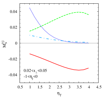
Figure 5: Prediction for the azimuthal moment $M_{N}^{\gamma j}$ at $\sqrt{s}=200$ GeV, as a function of $\eta_{\gamma}$, integrated over $-1\leq\eta_{j}\leq 0$ and $0.02\leq x_{\perp}\leq 0.05$. Solid line: using gluonic-pole cross sections. Dashed line: using standard partonic cross sections. Dotted line: maximum contribution from the gluon Sivers function (absolute value). Dot-dashed line: maximum contribution from the Boer-Mulders function (absolute value).

In conclusion, we have examined the azimuthal moment $M_{N}^{\gamma j}$, defined in Eq. (3), for the process $p^{\uparrow}p\to\gamma\,{\rm jet}\,X$. We have shown that in the kinematical regime of large and positive photon pseudorapidities and negative jet pseudorapidities, the moment is dominated by the quark Sivers function combined with the gluon unpolarized distribution function. The involved partonic subprocess is $qg\to\gamma q$. The two functions have to be convoluted with a gluonic-pole cross section instead of a standard partonic cross section, to take into account the presence of past-pointing and future-pointing Wilson lines arising from gluon interactions with the incoming gluon and the outgoing quark, respectively. The color structure of QCD implies that the gluonic-pole cross section for $qg\to\gamma q$ is equal to $-5/4$ times the standard partonic cross section. This leads to the robust prediction of a negative sign for the azimuthal moment $M_{N}^{\gamma j}$ in the considered kinematical regime, opposite to the expectation of the generalized parton model, obtained using standard partonic cross sections. The experimental measurement of $M_{N}^{\gamma j}$, possible at RHIC, will therefore be of crucial importance to deepen our present understanding of single-spin asymmetries.

This work is part of the EU Integrated Infrastructure Initiative Hadron Physics (RII3-CT-2004-506078). The work of C. B. is supported by the Dutch Foundation for Fundamental Research of Matter (FOM) and the Dutch National Organization for Scientific Research (NWO).

References

- Adams et al. (1991) D. L. Adams et al. (E704), Phys. Lett. B264, 462 (1991); J. Adams et al. (STAR), Phys. Rev. Lett. 92, 171801 (2004); S. S. Adler et al. (PHENIX), Phys. Rev. Lett. 95, 202001 (2005).
- Airapetian et al. (2005) A. Airapetian et al. (HERMES), Phys. Rev. Lett. 94, 012002 (2005); V. Y. Alexakhin et al. (COMPASS), Phys. Rev. Lett. 94, 202002 (2005); E. S. Ageev et al. (COMPASS), Nucl. Phys. B765, 31 (2007).
- Qiu and Sterman (1999) J.-W. Qiu, G. Sterman, Phys. Rev. D59, 014004 (1999).
- Bacchetta et al. (2005) A. Bacchetta, C. J. Bomhof, P. J. Mulders, F. Pijlman, Phys. Rev. D72, 034030 (2005).
- Kouvaris et al. (2006) C. Kouvaris, J.-W. Qiu, W. Vogelsang, F. Yuan, Phys. Rev. D74, 114013 (2006).
- Anselmino et al. (2006) M. Anselmino et al., Phys. Rev. D73, 014020 (2006); U. D’Alesio, F. Murgia, Phys. Rev. D70, 074009 (2004); M. Anselmino, M. Boglione, U. D’Alesio, E. Leader, F. Murgia, Phys. Rev. D71, 014002 (2005a).
- Brodsky et al. (2002) S. J. Brodsky, D. S. Hwang, I. Schmidt, Phys. Lett. B530, 99 (2002).
- Ji and Yuan (2002) X. Ji, F. Yuan, Phys. Lett. B543, 66 (2002); A. V. Belitsky, X. Ji, F. Yuan, Nucl. Phys. B656, 165 (2003); D. Boer, P. J. Mulders, F. Pijlman, Nucl. Phys. B667, 201 (2003).
- Collins (2002) J. C. Collins, Phys. Lett. B536, 43 (2002).
- Efremov et al. (2005) A. V. Efremov, K. Goeke, S. Menzel, A. Metz, P. Schweitzer, Phys. Lett. B612, 233 (2005).
- Bomhof et al. (2007) C. J. Bomhof, P. J. Mulders, W. Vogelsang, F. Yuan Phys. Rev. D75, 074019 (2007).
- Bomhof et al. (2004) C. J. Bomhof, P. J. Mulders, F. Pijlman, Phys. Lett. B596, 277 (2004); Eur. Phys. J. C47, 147 (2006).
- Sivers (1990) D. W. Sivers, Phys. Rev. D41, 83 (1990).
- Vogelsang and Yuan (2005) W. Vogelsang, F. Yuan, Phys. Rev. D72, 054028 (2005).
- Boer and Vogelsang (2004) D. Boer, W. Vogelsang, Phys. Rev. D69, 094025 (2004).
- Boer (1999) D. Boer, Phys. Rev. D60, 014012 (1999); M. Anselmino, U. D’Alesio, F. Murgia, Phys. Rev. D67, 074010 (2003).
- Schmidt et al. (2005) I. Schmidt, J. Soffer, J.-J. Yang, Phys. Lett. B612, 258 (2005).
- Bacchetta et al. (2004) A. Bacchetta, U. D’Alesio, M. Diehl, C. A. Miller, Phys. Rev. D70, 117504 (2004).
- Boer and Mulders (1998) D. Boer, P. J. Mulders, Phys. Rev. D57, 5780 (1998).
- Bomhof and Mulders (2007) C. J. Bomhof, P. J. Mulders, JHEP 02, 029 (2007).
- Gluck et al. (1998) M. Glück, E. Reya, A. Vogt, Eur. Phys. J. C5, 461 (1998).
- Anselmino et al. (2005b) M. Anselmino et al., Phys. Rev. D72, 094007 (2005b).
- Collins et al. (2006) J. C. Collins et al., Phys. Rev. D73, 014021 (2006).
- Soffer (1995) J. Soffer, Phys. Rev. Lett. 74, 1292 (1995).
- Gluck et al. (2001) M. Glück, E. Reya, M. Stratmann, W. Vogelsang, Phys. Rev. D63, 094005 (2001).
- Bacchetta et al. (2000) A. Bacchetta, M. Boglione, A. Henneman, P. J. Mulders, Phys. Rev. Lett. 85, 712 (2000).
- Anselmino et al. (2005c) M. Anselmino et al., Phys. Rev. D71, 074006 (2005c).