Reply to: ”Improved Determination of the CKM Angle $\alpha$ from $B\to\pi\pi$ decays”

Abstract

In reply to Ref. nimportenawak we demonstrate why the arguments made therein do not address the criticism exposed in Ref. bayestrouble on the fundamental shortcomings of the Bayesian approach when it comes to the extraction of parameters of Nature from experimental data. As for the isospin analysis and the CKM angle $\alpha$ it is shown that the use of uniform priors for the observed quantities in the Explicit Solution parametrization is equivalent to a frequentist construction resulting from a change of variables, and thus relies neither on prior PDFs nor on Bayes’ theorem. This procedure provides in this particular case results that are similar to the Confidence Level approach, but the treatment of mirror solutions remains incorrect and it is far from being general. In a second part it is shown that important differences subsist between the Bayesian and frequentist approaches, when following the proposal of Ref. nimportenawak and inserting additional information on the hadronic amplitudes beyond isospin invariance. In particular the frequentist result preserves the exact degeneracy that is expected from the remaining symmetries of the problem while the Bayesian procedure does not. Moreover, in the Bayesian approach reducing inference to the 68% or 95% credible interval is a misconception of the meaning of the posterior PDF, which in turn implies that the significant dependence of the latter to the chosen parametrization cannot be viewed as a minor effect, contrary to the claim in Ref. nimportenawak .

I Introduction

In Ref. bayestrouble we have shown through the example of the extraction of the Cabibbo-Kobayashi-Maskawa (CKM) angle $\alpha$ from $B\to\pi\pi,\,\rho\rho$ decays that the Bayesian treatment as done, e.g., by the UTfit collaboration UTfitpapers , suffers from major difficulties. The problems we have found are related to the presence of unknown free parameters which should actually be constrained by the data. We have shown that the results of the Bayesian analysis depend on the priors and the chosen parameterization in an uncontrollable manner, and may even diverge in some cases. Furthermore we have demonstrated that the priors cannot always be specified in a consistent way with respect to the symmetries of the problem, which results in the present example in an incorrect description of the $\alpha\to 0$ limit.

The authors of Ref. nimportenawak replied to our criticism. In the first part of their paper they agree with us on the dependence of the analysis with respect to the choice of priors and parameterization, even when the data are sufficiently precise so that the posterior PDFs are contained in the corresponding prior ranges. Ref. nimportenawak claims that this should not be viewed as a fundamental drawback of the Bayesian treatment, because in the absence of additional information on the parameters one should use uniform priors on the quantities that are directly measured (what we have called the ”Explicit Solution” parameterization in bayestrouble ). We emphasize in the following that this recipe can only be (approximately) justified within the framework of classical statistics and is thus not actually Bayesian. Moreover, it is far from being general.

In the second part of Ref. nimportenawak it is argued that in addition to the isospin analysis one may use bounds on the magnitude of the fit parameters related to hadronic matrix elements, and when taken into account the Bayesian treatment behaves more reliably. While this new recommendation may appear physically sound, the problem reported in bayestrouble uses the original isospin analysis GL , where the hadronic parameters are unknown and only isospin symmetry is used. Changing the hypotheses cannot be considered as a satisfying answer to our findings: indeed the validity of the statistical approach must be proven independently of the problem at hand. Despite this inconsistency, we accept the new proposal and show below that even with the use of this additional information one finds important quantitative and qualitative differences between the frequentist and the Bayesian results.

In any case, the new recommendations of the UTfit collaboration for treating problems with a priori free unknown parameters differ quite importantly from their previous publications, which implies that the results published therein are obsolete. We are therefore expecting new analysis results for the angles $\alpha$ from $B\to\rho\pi$ and $\gamma$ from charmful modes, for which similar difficulties can be apprehended.

We conclude that Ref. nimportenawak does not abrogate our criticism, because the only known examples where the Bayesian treatment leads to a numerically reasonable result do not provide any general argument in favor of the underlying hypotheses. In contrast, the frequentist approach can handle many types of situations smoothly, independently of whether there are free parameters and/or theoretical uncertainties.

II The original isospin analysis

The term ”isospin analysis” (which in Ref. nimportenawak is replaced by “minimal assumptions”) refers to the original paper by Gronau and London GL . Within this framework, only isospin symmetry is used to parametrize the decay amplitudes. Although it is not an exact symmetry, its accuracy in $B\to\pi\pi$ is expected to be of the order of 1% GronauZupan (once the known dominant contribution from electroweak penguins has been taken into account) and is thus of phenomenological relevance. Neither the Standard Model nor isospin symmetry imply anything on the “natural” scale of the hadronic amplitudes.

In Ref. bayestrouble we showed that the Pivk-Le Diberder (PLD) and Explicit Solution (ES) parameterizations give the most reasonable answer for the Bayesian treatment, because the corresponding parameters are close or identical to the measured quantities. This is confirmed (for the ES parameterization) by the authors of Ref. nimportenawak , who thus agree on the fact that other parameterizations lead to unstable results. The better behavior of the ES description (which follows from our detailed analysis and should be acknowledged as such) can be easily understood as follows. Let us stick to the Gaussian case and first assume that there is no degeneracy so that the angle $\alpha$ is given by a known single-valued function of the observables. One can construct a sampling distribution for $\alpha$ as defined by its analytical expression by randomizing the observables according to Gaussian PDFs where the true (unknown) central values and standard deviations have been replaced by their corresponding measured estimators. It is then straightforward to show that the position of the peak and its width are consistent estimators of, respectively, $\alpha$ and its uncertainty. This procedure does not need to define priors nor integration on the true values of the parameters, and does not rely on Bayes’ theorem: it just follows from standard rules of classical statistics.

Technically this procedure can be reproduced by applying the “Bayesian” treatment of Ref. firstUTfit to the ES parameterization bayestrouble with uniform priors. Because for Gaussian measurements the standard deviation of a quantity is equal to the 68% CL frequentist error, it is not a surprise to have similar numbers in the ES parameterization between the “Bayesian” and frequentist treatments. The remaining differences, namely the fact that one finds exactly degenerate mirror solutions only in the frequentist approach, mainly come from the integration (logical AND) over mirror solutions in the randomization treatment, which results from an unacceptable interpretation of physical constants that could simultaneously take different values bayestrouble .

Besides, the Explicit Solution trick is not general enough to treat with “minimal assumptions” all the interesting physical problems. Even when there is the same number of parameters as the number of independent observables, there is no guarantee that the theoretical equations can be inverted to express the parameters as functions of the observables. The Gronau-London isospin analysis is quite special in this respect. More importantly, most of the time one has overconstrained systems, that is one has more observables than parameters. In this case no “Explicit Solution” parameterization exists, and no general probability argument would help to find what is the most “natural” parameterization for a Bayesian treatment with uniform priors.

To close this Section we point out two misconceptions in Ref. nimportenawak . The first one is related to the claim that the 68% or 95% confidence level or credible intervals are more meaningful than the full curve. The fact that experimental measurements are often summarized as one- or two standard deviation intervals is just a matter of convention and if the curve has a complicated shape, it cannot be reduced to a one or two-number description without loss of information. In particular for the present case, we emphasize the importance of having exactly degenerate peaks in the angle $\alpha$ (as are reproduced by the constrained frequentist fit, see below) to be in agreement with isospin symmetry no matter the values of the 68% or 95% error intervals.

The second misconception is related to the above misunderstanding of the meaning of the degeneracy that is intrinsic to the isospin analysis. The fact that with the new data from Summer 2006 HFAG one sees only four peaks instead of eight as a function of $\alpha$ is not related to the improved measurements, but to the fact that now the experimental central values are slightly outside the physical region that is defined by the isospin symmetry (which is related to the property that both the three amplitudes and their $CP$ conjugates must form a triangle in the complex plane). Most presumably the data will evolve in such a way that the eightfold ambiguity reappears, which is the general case in the mathematical sense, and not a “fortuitous accident” as claimed in nimportenawak . Would a different ambiguity pattern be confirmed by better data, then either the Standard Model or the isospin symmetry should be questioned.

III Adding external information

The authors of Ref. nimportenawak recommend that the “default” plot summarizing the present constraints on the angle $\alpha$ coming from $B\to\pi\pi$ decays should take into account additional theoretical and phenomenological information. The physical arguments that are presented in favor of such an approach are perfectly legitimate and we do not object them. However the problem that was studied in detail in bayestrouble is not this one, but rather the original isospin analysis. Let us recall the advantages of performing the analysis assuming only isospin symmetry.

• Neither isospin symmetry nor $B\to\pi\pi$ experimental measurements give any insight on the typical scale of the hadronic amplitudes; thus it is a natural choice for the experimental collaborations to present their results in a way that is independent of possible assumptions on the hadronic amplitudes.

• The original paper GL only assumed isospin symmetry.

• One can think of many relevant physical problems containing completely free unknown parameters, the typical scale of which is not controlled even as an order of magnitude. This is the case, e.g., of general Beyond the Standard Model scenarios where one parametrizes new arbitrary contributions with a few quantities that a priori can take any value. The original isospin analysis is thus a pedagogical example that exhibit many features that would appear in more general situations.

Having this in mind we can now examine the new proposal of Ref. nimportenawak . First we remark that the statement made in nimportenawak according to which one can get new constraints on $\alpha$, and eventually lift the degeneracies and suppress the solution at $\alpha\rightarrow 0$, provided one uses additional theoretical and phenomenological knowledge, is obviously trivial and was the guideline of, e.g., Section VI.1 of Ref. ThePapII and many similar studies in the past.

Second we stress that additional information is ill-defined. The assumptions made in nimportenawak are equivalent to an analysis with a finite theoretical error on each parameter (except the one that is scanned, here the angle $\alpha$), such as the “historical” determination of the Unitarity Triangle firstUTfit . It is well known that in general there is no unambiguous definition of the meaning of a theoretical error, and when such uncertainties are present the Bayesian and frequentist methods cannot be compared in a rigorous way. The authors of Ref. nimportenawak take as a strong argument in favor of their approach the fact that their results are weakly dependent of the assumed order of magnitude for the amplitudes. We do not find this convincing, but rather would like to take the following two limits, which to our knowledge are the only ones where the concept of a theoretical error becomes perfectly well defined.

• Theory errors go to zero, i.e. the corresponding parameters are fixed constants. In this case it is trivial to show that both frequentist and Bayesian approaches lead to equivalent numerical results.

• Theory errors go to infinity, i.e. the corresponding parameters are completely free unknowns; this is the case that is discussed in the previous section and where the Bayesian treatment in a generic parameterization simply fails.

Hence, only in the very specific case where both experimental and theoretical uncertainties are “sufficiently” reduced, and there is no free parameter, the numerical comparison of the Bayesian treatment with the frequentist classical approach may become meaningful, and in the Bayesian case one might expect a “reasonable” stability with respect to priors and parameterization. This stability, however, must be extensively checked case-by-case, which has not been done in the previous publications by the UTfit collaboration UTfitpapers .

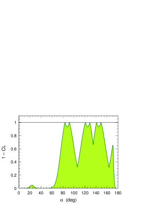
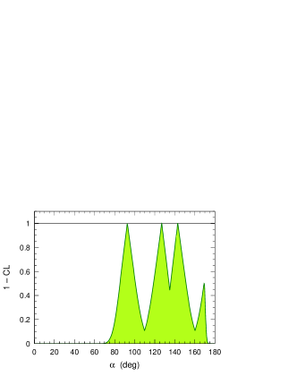
Figure 1: Frequentist confidence level as a function of the angle $\alpha$, taking into account the following constraints nimportenawak : $|T^{+-}|\leq 10$, $|T^{00}|\leq 10$ and $|P|\leq 2.5$ (natural units), for $B\to\pi\pi$ decays. Upper plot: data that correspond to the plots in Ref. bayestrouble , Lower plot: new data that correspond to Fig. 5 in nimportenawak .

Table 1: For each of the peaks in the plots of Fig. 1 are shown the corresponding values for the parameters as found by direct analytical calculation or by the numerical fit. The first six solutions correspond to the upper plot, while the three others correspond to the lower plot

Solution	$\alpha$	$|T^{+-}|$	$|T^{00}|$	$|P|$
1	$83.7^{\circ}$	$1.74$	$1.07$	$0.763$
2	$91.8^{\circ}$	$1.73$	$1.28$	$0.559$
3	$120.7^{\circ}$	$2.01$	$0.960$	$0.650$
4	$128.8^{\circ}$	$2.21$	$0.600$	$0.973$
5	$141.2^{\circ}$	$0.960$	$2.07$	$1.21$
6	$149.3^{\circ}$	$1.18$	$2.16$	$1.09$
1	$92.7^{\circ}$	$1.71$	$1.19$	$0.634$
2	$126.9^{\circ}$	$2.14$	$0.722$	$0.791$
3	$143.1^{\circ}$	$1.17$	$1.99$	$1.05$

Fig. 1 shows the results of a constrained frequentist fit that takes into account the same information on the hadronic parameters as in Fig. 5 of nimportenawak , namely that the amplitudes verify the following bounds: $|T^{+-}|\leq 10$, $|T^{00}|\leq 10$ and $|P|\leq 2.5$ (in natural units). In particular these bounds suppress the parameter configurations with $\alpha\to 0$, as emphasized in nimportenawak . Indeed this curve is not too different from the one that corresponds to the Bayesian treatment, however it appears clearly that the frequentist analysis, in contrast to the Bayesian one, respects the exact degeneracy between the mirror solutions that survive the phenomenological bounds, as requested by the symmetries of the problem. Table 1 shows the parameter values that correspond to each of the peaks in the plots of Fig. 1, as obtained analytically from the exact formulas or numerically from the fit. Since these parameter configurations all lead to the very same observables and all verify the phenomenological bounds advocated in Ref. nimportenawak , there is no way to tell which configuration is “more probable”. In turn, this means that the Bayesian treatment lifts the degeneracy only because of the unphysical marginalization over the hadronic parameters, and that reducing the output information to the 68% or 95% probability intervals is very misleading. From Table 1 one sees that to lift the degeneracy between the remaining solutions, even partially, one would need to know the amplitudes with a relative uncertainty of better than 100%, which is feasible using more dynamical approaches to hadronic elements, but which would request far more than just isospin symmetry and orders of magnitude for the hadronic amplitudes.

To close this section we emphasize that there are many interesting problems depending on completely unknown parameters on which we have no clue, not even a rough order of magnitude. This is for example the case in generic new physics scenarios, such as the one of the second paper of Ref. UTfitpapers . There arbitrary new physics contributions to $B\overline{B}$ mixing is parametrized by a quantity $C_{B}\,\exp(2i\phi_{B})$; by definition, since no assumption is made on specific new physics models, the analysis does not give any insight to the “natural” scale of the parameter $C_{B}$. Thus one again may expect the Bayesian treatment to suffer from instabilities when moving from, e.g, the $(C_{B},\phi_{B})$ to the $(x_{B}=c_{B}\cos\phi_{B},y_{B}=c_{B}\sin\phi_{B})$ parameterization (such instabilities are expected to increase with the number of new physics parameters). In other words the Bayesian approach as recommended by Ref. nimportenawak cannot be applied (although in practice it is) to the full generality of problems at hand.

- (1) M. Bona et al. [UTfit Collaboration], arXiv:hep-ph/0701204
- (2) J. Charles et al., arXiv:hep-ph/0607246
- (3) M. Bona et al. [UTfit Collaboration], JHEP 0507 (2005) 028; JHEP 0603 (2006) 080; JHEP 0610 (2006) 081
- (4) M. Gronau and D. London, Phys. Rev. Lett. 65 (1990) 3381
- (5) M. Gronau and J. Zupan, Phys. Rev. D 71 (2005) 074017
- (6) M. Ciuchini et al., JHEP 0107 (2001) 013
- (7) G. d’Agostini, Rep. Prog. Phys. 66 (2003) 1383
- (8) The Heavy Flavor Averaging Group, http://www.slac.stanford.edu/xorg/hfag/
- (9) J. Charles et al. [CKMfitter group], Eur. Phys. J. C 41 (2005) 1