Axial current matrix elements and pentaquark decay widths in chiral soliton models

Abstract

Here I explain why in chiral soliton models the hadronic transition operator of the pentaquark decay cannot be identified from the axial current.

I Introduction

Many computations of pentaquark widths in soliton models fully rely on adopting the axial current as the transition operator for the hadronic decay $\Theta^{+}\to KN$ Diakonov:1997mm ; Ellis:2004uz ; addrefs . These computations embody the $SU(3)$ generalization of the Goldberger–Treimann relation (GTR) between the nucleon axial charge ($g_{A}$) and the pion nucleon coupling constant ($g_{\pi NN}$) to map the soliton model onto a Yukawa interaction. These calculations have been criticized for inconsistencies with the large $N_{C}$ limit Itzhaki:2003nr . In that limit the $\Theta$ has a non–zero mass gap to the nucleon and hence a non–zero width. On the other hand, the Skyrme model $KN$ phase shifts are exactly known for $N_{C}\to\infty$ Karliner:1986wq ; Scoccola:1990pt . They do not exhibit pronounced (narrow) resonances. More recently a detailed analysis Walliser:2005pi showed that these phase shifts indeed contain the pentaquark exchange contribution. Most crucially the transition matrix element for $\Theta^{+}\to NK$ was extracted and established that it does not equal the axial current matrix element suggested by the generlized GTR. Thus any chiral soliton model calculation of the $\Theta^{+}$ width that is based on identifying the transition matrix element from the axial current must be strongly doubted. Given that this identification is continuously employed in soliton motivated studies Yang:2007yj ; Diakonov:2006kh ; Lorce:2006nq ; Praszalowicz:2006rt ; YKIS06 of pentaquark widths and that the resultant claim for the existence of narrow exotic baryons is airily adopted to this day Kuznetsov:2007dy , it occurs highly necessary to be emphatic on the arguments of ref. Walliser:2005pi .

Throughout I will discard flavor symmetry breaking. Though it is important for actual predictions to be reliable, it hides the main issue. Also, I will focus on the Skyrme model. Admittedly this model is insufficient in various aspects. Here the crucial point is the treatment of collective soliton excitations. This is completely independent of the specific underlying effective meson theory. It is thus advantageous to consider the simplest model available.

II Decay widths from axial current matrix elements

Models with explicit baryon ($B$) and meson ($\Phi$) fields commonly have tri–linear Yukawa interactions (the fields are multi–valued in flavor space),

$$\mathcal{L}_{\rm int}=\frac{g_{\phi BB^{\prime}}}{M_{B}+M_{B}^{\prime}}\,\bar{\Psi}_{B}\gamma_{5}\gamma_{\mu}\left(\partial^{\mu}\Phi\right)\Psi_{B^{\prime}}\,.$$ (1)

The derivative interaction reflects chiral symmetry and $\gamma_{5}$ the pseudoscalar nature of the considered meson. The Yukawa coupling leads to the standard width

$$\Gamma(B^{\prime}\to B\Phi)=\frac{\overline{|\mathcal{M}|^{2}}}{8\pi M_{B}M_{B^{\prime}}}\,|\vec{p}_{\Phi}|$$ (2)

where $\mathcal{M}$ is the matrix element resulting from eq. (1). The overbar denotes summing and averaging over spins. The details of this matrix element depend on the spins of the considered baryons. It suffices to keep in mind that $\mathcal{M}$ is linear in both, the coupling $g_{\phi BB^{\prime}}$ and the momentum of the final meson, $\vec{p}_{\Phi}$. The latter property results from the pseudoscalar nature of $\Phi$. So we have $\Gamma\propto g_{\phi BB^{\prime}}^{2}|\vec{p}_{\Phi}|^{3}$. The Yukawa model reflects the GTR between the Yukawa coupling $g_{\pi NN}$ and the axial charge of the nucleon, $g_{A}$

$$f_{\pi}g_{\pi NN}=M_{N}g_{A}\,.$$ (3)

This relation heavily relies on PCAC which expresses the non–conservation of the axial current

$$\partial^{\mu}A_{\mu}^{a}(x)=f_{a}m_{a}^{2}\phi^{a}(x)\,,$$ (4)

where $a$ is the flavor index.

In soliton models the situation is considerably different. Only meson fields are fundamental while baryons emerge as (topological) configurations thereof that solve the (classical) field equations. To study meson baryon interactions, asymptotic meson states are constructed from small amplitude fluctuations about the soliton that describes the baryon. An immediate puzzle arises. Since the soliton is a stationary point, no term linear in the meson fluctuations exists. Hence there is no obvious coupling constant $g_{\phi BB^{\prime}}$ and profound assumptions are necessary to make use of eq. (2). The profound assumption often made in soliton models is to evaluate $g_{A}^{BB^{\prime}}$ (the axial current transition matrix element), use eq. (3) to identify $g_{\phi BB^{\prime}}$ and substitute it into eq. (2) to compute the decay width. This is an attempt to map the soliton model onto the Yukawa model. Certainly, one must ask for the role of the GTR in soliton models. Before doing so, we will outline the computations of $g_{A}$, $g_{\pi NN}$ and its $SU(3)$ relatives from GTR.

Starting point is the hedgehog configuration $U_{0}(\vec{x})={\rm exp}\left[i\hat{\vec{x}}\cdot\vec{\tau}F(r)\right]$, that solves the classical field equations. In the next step collective coordinates $A(t)\in SU(3)$ are introduced via

$$U(\vec{x},t)=A(t)U_{0}(\vec{x})A^{\dagger}(t)\,.$$ (5)

Note that this configuration does not solve the stationary conditions, eventually this gives rise to terms linear in the meson fields. The $A(t)$ are treated quantum mechanically to generate states with good spin and flavor quantum numbers. Baryon wave–functions $\Psi_{B}(A)=\langle A|B\rangle$ emerge in the space of the collective coordinates. In the absence of flavor symmetry breaking these wave–functions are classified with respect to $SU(3)$ flavor multiplets; spin $\frac{1}{2}$ states in the octet, anti–decuplet; spin $\frac{3}{2}$ in the decuplet; etc.. This treatment is called the rigid rotator approach.

In the rigid rotator approach the axial current operator has the model independent from

$$A_{i}^{a}=\sum_{k=1,2,3}A^{(0)}_{ik}\,(\vec{x})D_{ak}+\sum_{\genfrac{}{}{0.0pt}{}{k=1,2,3}{\alpha,\beta=4,\ldots,7}}A^{(1)}_{ik}(\vec{x})\,d_{k\alpha\beta}D_{a\alpha}R_{\beta}+\sum_{k=1,2,3}A^{(2)}_{ik}(\vec{x})\,D_{a8}R_{k}$$ (6)

up to omitted flavor symmetry breaking. The structure of the coefficient functions is $A^{(m)}_{ik}(\vec{x})=A_{1}^{(m)}(r)\delta_{ik}+A_{2}^{(m)}(r)\hat{x}_{i}\hat{x}_{k}$. The $A_{1,2}^{(m)}(r)$ are radial functions through the profile function $F(r)$. The $D_{ab}={\scriptstyle\frac{1}{2}}{\rm tr}\left(\lambda_{a}A\lambda_{b}A^{\dagger}\right)$ and the $R_{a}$ are the adjoint representation of the $SU(3)$ collective coordinates and the intrinsic $SU(3)$ generators, respectively. It is legitimate to use isospin invariance and compute $g_{A}$ as the nucleon matrix element $\langle 2A_{3}^{3}\rangle$. Then eq. (3) implies Diakonov:1997mm ; Ellis:2004uz

$$g_{\pi NN}=\frac{7}{10}\left[G_{0}+\frac{1}{2}G_{1}+\frac{1}{14}G_{2}\right]\qquad{\rm with}\qquad G_{m}=-\frac{8\pi M_{N}}{3f_{\pi}}\int_{0}^{\infty}drr^{2}\left[A_{1}^{(m)}(r)+\frac{1}{3}A_{2}^{(m)}(r)\right]\,.$$ (7)

The relative coefficients stem from the nucleon matrix elements of the collective coordinate operators in eq. (6). They are readily obtained from $SU(3)$ Clebsch–Gordan coefficients, e.g. $\langle p\uparrow|D_{33}|p\uparrow\rangle=-7/30$. Generalizing the above result for $g_{\pi NN}$ to flavor $SU(3)$ yields coupling constants

$$G_{10}=G_{0}+\frac{1}{2}G_{1}\qquad{\rm and}\qquad G_{\overline{10}}=G_{0}-G_{1}-\frac{1}{2}G_{2}$$ (8)

that (under the GTR assumption) respectively measure the coupling of baryons from the decuplet ($\Delta$) and the anti–decuplet ($\Theta^{+}$) to those in the octet (nucleon, hyperons). These coupling constants enter the matrix element $\mathcal{M}$ and predict widths for hadronic baryon decays via eq. (2): $\Gamma(\Delta\to N\pi)\propto G_{10}^{2}|\vec{p}_{\pi}|^{3}$ and $\Gamma(\Theta^{+}\to NK)\propto G_{\overline{10}}^{2}|\vec{p}_{K}|^{3}$. The omitted constants of proportionality are merely kinematical factors misconduct . Model calculations Kanazawa:1987uv ; Blotz:1994wi ; Weigel:1995cz indicate that $G_{0}$ and $G_{1}$ are comparable. That is, significant cancellations cause $G_{\overline{10}}$ to be rather small. This has been the main argument for claiming a $\Theta^{+}$ width of the order of only a few ${\rm MeV}$, or even less. The cancellations between $G_{0}$ and $G_{1}$ persist when the number ($N_{C}$) of color degrees of freedom is sent to infinity Praszalowicz:2003tc . This completes the way of thinking about pentaquark decay widths put forward in refs. Diakonov:1997mm ; Ellis:2004uz and frequently adopted later on addrefs . A couple of issues doubt this approach already afore we test it against incontrovertible results from the phase shift analysis:

• The classical field equations affect only the first part $\partial_{i}A^{(0)}_{ik}=\mathcal{O}\left(m_{\pi}^{2}\right)$ while the last term ($A^{(2)}$) vanishes or is at least small because it essentially is the axial singlet matrix element. On the other hand $\partial_{i}A^{(1)}_{ik}$ is not part of any equation of motion. Hence the axial current computed solely from the classical profile functions violates PCAC Weigelappendix . As a consequence, the use of GTR in $SU(3)$ soliton models is questionable because a major entry is not met.

• The above derivation only involves the classical soliton and there is no reference to asymptotic meson states. In two flavor soliton models the GTR arises from the long range behavior of the soliton profile Adkins:1983ya and has been identified from one–pion exchange contribution to the nucleon–nucleon interaction. However, this process does not require asymptotic pion states. Also, that argument strongly relies on pions being massless. For $m_{\pi}>0$, $g_{A}$ cannot be read off from the long range behavior and thus not be related to $g_{\pi NN}$.

It is thus not surprising that $SU(3)$ Skyrme model calculations severely fail to reproduce GTR when $g_{\pi NN}$ is identified from the long range behavior of the soliton Kanazawa:1987uv . Evidently, it is not possible to directly map soliton models onto the Yukawa model.

III Rotation–vibration coupling and $KN$ scattering

In principle, it must be possible to extract $\Theta^{+}$ properties from kaon nucleon scattering data. After all, that is the process in which resonances are to be observed. This process can be studied within a given soliton model without reference to the Yukawa model. The corresponding phase shifts have been computed in the Skyrme model Karliner:1986wq ; Scoccola:1990pt within the so–called adiabatic approximation, which neglects the dynamical properties of the collective modes. This model treatment is exact to first non–trivial order in the large–$N_{C}$ expansion. A typical Skyrme model result is shown as total phase shift in figure 1.

                 

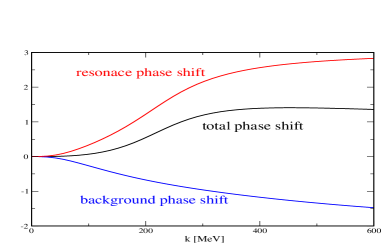
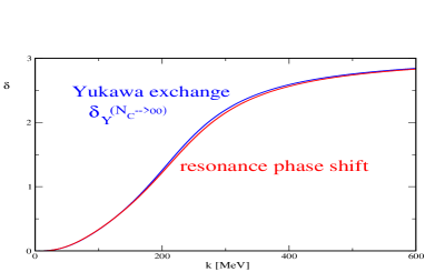
Figure 1: Skyrme model results for momentum dependent phase shifts in the $\Theta^{+}$ channel. The ’total phase shift’ is the result in adiabatic approximation, the ’background phase shift’ describes scattering in the space orthogonal to the soliton’s rigid rotation and the ’resonance phase shift’ is their difference, compared to the Yukawa exchange contribution (10,11) in the right panel. The pictures are adopted from ref. Weigel:2006vt .

Since this is exact to $\mathcal{O}\left(N_{C}^{0}\right)$, any treatment (that might include subleading pieces) of collective degrees of freedom in the Skyrme model must reproduce this phase shift in the limit $N_{C}\to 0$. This concerns the full momentum dependence and not only an attempt to match a single parameter Diakonov:2006kh .

From figure 1 the immediate question arises whether or not the pentaquark channel resonates as $N_{C}\to\infty$. If at all, this concerns the collective modes, eq. (5). As a first response to this question, one may constrain the small amplitude fluctuation to be orthogonal to the collective modes. The phase shift computed from these restricted fluctuations is shown as the background phase shift in figure 1. Its difference to the total phase shift defines the resonance phase shift. Obviously the latter resonates, though it is definitely not narrow. Of course, the challenge is to verify that this resonance phase shift arises from the exchange of the collective excitation $\Theta^{+}$. Then collective modes must be treated dynamically within the scattering problem. This was done in ref. Walliser:2005pi by considering vibrations ($\widetilde{\eta}$) about the rotating hedgehog, (The interested reader should consult that paper for quantitative results, particularly for the realistic case $N_{C}=3$ and $m_{K}\neq m_{\pi}$.). The configuration (5) does not solve the stationary conditions, this will now give rise to terms linear in $\widetilde{\eta}$ that couple to the collective coordinates and their time derivative. The constraints that ensure $\widetilde{\eta}$ to be orthogonal to the collective modes, yield additional linear terms. After quantization, the linear terms contain only a single collective coordinate operator

$$\hat{X}_{ak}=\sum_{\alpha,\beta=4,\ldots,7}d_{k\alpha\beta}D_{a\alpha}R_{\beta}\,.$$ (9)

This operator also occurs in the axial current operator, eq. (6). In the limit $N_{C}\to\infty$ the Schrödinger equation for $\widetilde{\eta}$ has a very simple solution Walliser:2005pi : $|\widetilde{\eta}\rangle=|\eta\rangle-|z\rangle\langle\eta|z\rangle$, where $\langle\vec{x}|\eta\rangle$ is the wave function in the adiabatic approximation and $\langle\vec{x}|z\rangle$ is the (properly normalized) wave function that represents the collective modes. Since $\langle\vec{x}|z\rangle$ is determined by the soliton configuration it is localized in space. Thus $\langle\vec{x}|\eta\rangle$ and $\langle\vec{x}|\widetilde{\eta}\rangle$ behave identically in the asymptotic regime and $\widetilde{\eta}$ indeed reproduces the total phase shift of figure 1 as $N_{C}\to\infty$. To extract the information about the collective excitations that is contained in $\widetilde{\eta}$, it is fruitful to introduce fluctuations $\overline{\eta}$ which are the solution to the Schrödinger equation with $\hat{X}\to 0$, i.e. without coupling to the collective coordinates. The so–generated equation of motion is that from the adiabatic approximation augmented by the constraints. Hence the $\overline{\eta}$ phase shift is the background phase shift in figure 1. In the full $\widetilde{\eta}$ problem the effect of non–zero $\hat{X}$ is to add the resonance phase shift $\delta_{Y}(k)$ to the $\overline{\eta}$ phase shift with

$${\rm tan}\left(\delta_{Y}(k)\right)=\frac{\Gamma(\omega_{k})/2}{\omega_{\Theta}-\omega_{k}+\Delta(\omega_{k})}\,.$$ (10)

Here $\omega_{\Theta}$ is the excitation energy of the pentaquark as computed in the rigid rotator approach while $\Delta$ denotes the energy shift. Numerically $\Delta$ turns out to be negligibly small. This shows that the rigid rotator approach reliably predicts the pentaquark mass (in a model) sigma . The width function

$$\Gamma(\omega_{k})=2k\omega_{0}X_{\Theta}^{2}\left|\langle\overline{\eta}_{\omega_{k}}|(2\lambda)|z\rangle\right|^{2}$$ (11)

describes the (Yukawa) exchange contribution of a pentaquark to kaon–nucleon scattering. Here, the explicit expressions for the normalization factor $\omega_{0}$ and the radial function $\lambda$ are of minor importance. For $N_{C}\neq 3$ the low–lying $SU(3)$ representations are no longer octet, decuplet, anti–decuplet etc.. This induces $N_{C}$ dependences for $\Psi_{A}$, the energy eigenvalues such as $\omega_{\Theta}$, and the matrix element $X_{\Theta}=\sqrt{\frac{32}{N_{C}}}\langle\Theta^{+}\uparrow|X_{43}+iX_{53}|n\uparrow\rangle$ turns into a function of $N_{C}$. It is normalized such that $\lim_{N_{C}\to\infty}X_{\Theta}=1$.

IV Comparison and Critique

The right panel of figure 1 shows the Yukawa–exchange phase shift as numerically computed from eq. (11) for $N_{C}\to\infty$. Obviously and most importantly it exactly matches the resonance phase shift! Unambiguously $\Gamma(\omega_{k})$ is the correct width function in this model (at least for $N_{C}\to\infty$). It is evidently very different from the width function computed via GTR from the axial current. Most remarkably $\Gamma(\omega_{k})$ contains only a single collective coordinate operator. Thus there cannot be any cancellation that would yield a small width.

There is a self–explanatory and rigorous reason for the appearance of only a single collective coordinate structure in the transition operator. To make contact with the adiabatic approximation (that is exact as $N_{C}\to\infty$), the equations of motion for the fluctuations are solved in the body–fixed frame, wherein the fluctuations rotate along with the soliton, eq. (5). In these equations the collective coordinates can only show up via the angular velocities, $\Omega_{a}=-i{\rm tr}\left[\lambda_{a}A(t)\dot{A}^{\dagger}(t)\right]$. Upon quantization the $\Omega_{a}$ are replaced by the generators $R_{a}$. Without the $D_{ab}$ available, there is only one possible kaon $P$–wave coupling which is Hermitian and behaves properly under $SU(3)$: $\sum\hat{x}_{k}\,d_{k\alpha\beta}\eta_{\alpha}R_{\beta}$. Subsequently matrix elements for the lab–frame fluctuations $\xi_{a}=D_{ab}\eta_{b}$ are required. This leads to $\hat{X}$ as the only allowed operator. Since this argument is irrespective of the considered chiral soliton model, the emergence of only a single collective coordinate operator for the hadronic transition $\Theta\to KN$ is common to all chiral soliton models.

The detailed analysis Walliser:2005pi of $\Gamma(\omega_{k})$ reveals a few more discrepancies to the axial current approach. The $|\vec{p}_{K}|^{3}$ behavior is seen only in the energy regime slightly above threshold; at larger energies is levels off. Though the correct width function does definitely not contain a $G_{0}$ type piece, it it seems plausible to identify the $G_{1}$ contribution with $\Gamma(\omega_{k})$ in the plane wave approximation in the $\vec{p}_{K}\to 0$ limit because it contains the same collective coordinate operator. However, the actual computation shows that the integrands of the spatial integrals differ by a factor ${\rm cos}(F/2)$.

When symmetry breaking is included, the $\Lambda$ channel must be incorporated to reproduce the correct total phase shift when $N_{C}\to\infty$. Also an additional collective coordinate operator $\hat{Y}_{ak}=\sum_{\alpha,\beta=4,\ldots,7}d_{k\alpha\beta}D_{a\alpha}D_{8\beta}$ emerges. In the large–$N_{C}$ limit it behaves similarly to the $G_{0}$ type piece, but in general no relation can be made.

V A note on $\Delta$

Many approaches describe the width of the $\Delta$ resonance via Yukawa interaction in pion nucleon scattering; thereby generalizing the GTR. This stimulates to discuss the consequences of the above results for the soliton model description of the $\Delta$ width.

The treatment that consistently describes the $\Theta$ width is characterized by essentially two features. First, the space of fluctuations is parted into a piece that contains collective modes and its orthogonal subspace. Only the latter contains to scattering meson states. For pion nucleon scattering this partition is not as problematic as for three flavor processes because the Wess–Zumino term can be ignored. Then terms that are subleading in the $1/N_{C}$ expansion and quadratic in the fluctuations emerge that couple these two subspaces. They are thus linear in the small amplitude fluctuations that describe asymptotic pion fields. Second, the collective modes are integrated out similar to the Lee–model approach Henley:1962 . This induces a separable potential for the fluctuations in the orthogonal subspace. Treated in an $R$–matrix formalism, this potential yields the resonance phase shift. As is deduced from the pentaquark problem the $R$–matrix elements must be evaluated from fluctuation wave–functions that are distorted by the classical soliton; the plain wave approximation is inconsistent with the partitioning of the fluctuation space. So far this agenda has not been fully carried out for the $\Delta$ resonance. The study of chapter 10 in ref. Schwesinger:1988af seems to come closest. Even though those results for the pion nucleon scattering amplitude in the $\Delta$ channel agree reasonably well with data, it should be stressed that they are obtained in the plain wave approximation, just criticized. Interestingly enough this approach does not generate a $\pi NN$ vertex Saito:1987uh ; Holzwarth:1990ym , irregardless of the plain wave approximation. Stated otherwise, the scenario that potentially describes the $\Delta$ resonance well, or at least consistently in a given soliton model, does not alter the pion nucleon coupling constant that is basic to GTR, eq. (3). So, as in the pentaquark channel, the soliton model computation of the $\Delta$ width does not proceed by generalizing the GTR. This is no contradiction to fundamental concepts of hadron physics because sandwiching the PCAC relation (4) between states other than the nucleon (and its octet partners) is impossible without assumptions about the nature of these states. For example, regarding $g_{\pi NN}$ and $g_{\pi N\Delta}$ with equal rigor, implies that the $\Delta$ would be an asymptotic state, yet it is a resonance. We note, however, that the GTR is indeed reproduced in the soliton model description of the nucleon–nucleon potential Adkins:1983ya ; Jackson:1985bn .

VI Conclusions

Here I have argued that pentaquark widths may not be computed from axial current matrix elements in chiral soliton models. The model prediction for the kaon nucleon phase shift is known in limit $N_{C}\to\infty$ and the axial current approach evidently fails to reproduce it. Though this fact is known for some time, this short discussion occurred necessary because this erroneous identification keeps on being applied. In chiral soliton models pentaquark widths (probably neither those of other baryon resonances) should not be estimated by mapping onto the Yukawa model via the GTR. Since the so–computed pentaquarks widths are not reliable predictions, the non–observation of such a narrow resonance (which seems more or less certain by now Hicks:2007vg ) should not be used against the chiral soliton picture for baryons. The statement that chiral soliton models predict a very narrow pentaquark baryon in the $S=+1$ channel essentially is a myth.

References

- (1) D. Diakonov, V. Petrov and M. V. Polyakov, Z. Phys. A 359 (1997) 305 [arXiv:hep-ph/9703373].
- (2) J. R. Ellis, M. Karliner and M. Praszałowicz, JHEP 0405 (2004) 002 [arXiv:hep-ph/0401127].
-
(3)
Many additional references on this approach can be traced from
http://www.rcnp.osaka-u.ac.jp/~hyodo/research/Thetapub.html. - (4) G. S. Adkins, C. R. Nappi and E. Witten, Nucl. Phys. B 228 (1983) 552.
- (5) N. Itzhaki, I. R. Klebanov, P. Ouyang and L. Rastelli, Nucl. Phys. B 684 (2004) 264 [arXiv:hep-ph/0309305].
- (6) N. N. Scoccola, Phys. Lett. B 236 (1990) 245.
- (7) M. Karliner and M. P. Mattis, Phys. Rev. D 34 (1986) 1991.
- (8) H. Walliser and H. Weigel, Eur. Phys. J. A 26 (2005) 361 [arXiv:hep-ph/0510055].
- (9) G. S. Yang, H. C. Kim and K. Goeke, Phys. Rev. D 75 (2007) 094004 [arXiv:hep-ph/0701168].
- (10) D. Diakonov, arXiv:hep-ph/0610166.
-
(11)
C. Lorce, Phys. Rev. D 74 (2006) 054019
[arXiv:hep-ph/0603231].
arXiv:0705.1505 [hep-ph]. - (12) M. Praszalowicz, AIP Conf. Proc. 828 (2006) 394.
- (13) Presentations by D. Diakonov, H. C. Kim and M. Praszałowicz at the YKIS06 conference, Osaka, Nov. 2006. http://www2.yukawa.kyoto-u.ac.jp/~ykis06/index.html
-
(14)
V. Kuznetsov, M. Polyakov, T. Boiko, J. Jang, A. Kim, W. Kim and A. Ni,
arXiv:hep-ex/0703003.
K. Piesciuk and M. Praszalowicz, arXiv:0704.0196 [hep-ph].
H. C. Kim, G. S. Yang and K. Goeke, arXiv:0704.1777 [hep-ph]. -
(15)
Ambiguities in the non–relativistic reduction thereof and associated
controversies are not subject of this discussion. They are documented in
H. Weigel, Eur. Phys. J. A 2 (1998) 391 [arXiv:hep-ph/9804260];
R. L. Jaffe, Eur. Phys. J. C 35 (2004) 221 [arXiv:hep-ph/0401187]; arXiv:hep-ph/0405268;
D. Diakonov, V. Petrov and M. Polyakov, arXiv:hep-ph/0404212. - (16) M. Praszałowicz, Phys. Lett. B 583 (2004) 96 [arXiv:hep-ph/0311230].
- (17) A. Kanazawa, Prog. Theor. Phys. 77 (1987) 1240.
- (18) A. Blotz, M. Praszałowicz and K. Goeke, Phys. Rev. D 53 (1996) 485 [arXiv:hep-ph/9403314].
- (19) For a review see H. Weigel, Int. J. Mod. Phys. A 11 (1996) 2419 [arXiv:hep-ph/9509398].
- (20) Induced kaon fields were considered as an early attempt to solve the problem, cf. appendix C in ref. Weigel:1995cz .
- (21) H. Weigel, Eur. Phys. J. A 31 (2007) 495 [arXiv:hep-ph/0610123]; arXiv:0704.2281 [hep-ph].
- (22) This does not justify to relate mass parameters to other predictions of the rigid rotator approach. The latter themselves may suffer severe ambiguities. An exemplary such prediction is the pion nucleon term that has been frequently employed to estimate the pentaquark mass Diakonov:1997mm ; Ellis:2004uz ; addrefs ; Yang:2007yj . However, the rigid rotator prediction for the term is subject to difficult to handle quantum corrections Meier:1996ng .
- (23) F. Meier and H. Walliser, Phys. Rept. 289 (1997) 383 [arXiv:hep-ph/9602359].
- (24) E. M. Henley and W. Thirring, Elementary Qunatum Field Theory, ch. 13. McGraw-Hill, 1962.
- (25) B. Schwesinger, H. Weigel, G. Holzwarth, and A. Hayashi, Phys. Rept. 173 (1989) 173.
- (26) S. Saito, Prog. Theor. Phys. 78 (1987) 746.
- (27) G. Holzwarth, Phys. Lett. B241 (1990) 165.
- (28) H. Verschelde, Phys. Lett. B 232 (1989) 15.
- (29) A. Jackson, A. D. Jackson, and V. Pasquier, Nucl. Phys. A432 (1985) 567.
-
(30)
K. Hicks,
arXiv:hep-ph/0703004.
M. Danilov and R. Mizuk, arXiv:0704.3531 [hep-ex].