LTH 738

NSF-KITP-07-13

The Effective Potential, the Renormalisation Group and Vacuum Stability

Martin B. Einhorn

Kavli Institute for Theoretical Physics, University of California, Santa Barbara CA 93106-4030, USA.

and D. R. Timothy Jones

Dept. of Mathematical Sciences, University of Liverpool, Liverpool L69 3BX, UK.

We review the calculation of the the effective potential with particular emphasis on cases when the tree potential or the renormalisation-group-improved, radiatively corrected potential exhibits non-convex behaviour. We illustrate this in a simple Yukawa model which exhibits a novel kind of dimensional transmutation. We also review briefly earlier work on the Standard Model. We conclude that, despite some recent claims to the contrary, it can be possible to infer reliably that the tree vacuum does not represent the true ground state of the theory.

1 Introduction

The effective potential $V(\phi)$ has proved to be an invaluable tool for investigating the nature of the vacuum state in weakly coupled quantum field theories. There is a well defined prescription [1],[2]  facilitating the perturbative calculation of $V(\phi)$, and a large literature of such calculations for various field theories including the Standard Model (SM) [3] and the Minimal Supersymmetric Standard Model (MSSM) [4]. Theoretical forays into the Early Universe frequently involve the effective potential and, for example, transition from an unstable or metastable state by tunnelling or “slow-roll”.[5],[6]. New scalar excitations such as the inflaton are hypothesised to lead to the desired behaviour.[7].

In this article, we confine ourselves largely to one specific topic: the destabilisation of a tree-level vacuum by radiative corrections. In the SM, it has been argued that, if the fermion loop contribution (dominated by the top quark) to the one-loop potential were large enough then the electroweak vacuum would be destabilised, due to the existence of a deeper minimum at large $\phi$; this phenomenon is translated into a lower limit on the Higgs mass as a function of the top quark mass [8]-[19].

The electroweak minimum of the SM is a consequence of the choice $m^{2}<0$ for the Higgs mass parameter. As a result the perturbative definition of $V(\phi)$ is non-convex (in the tree approximation) and develops an imaginary part for small values of $\phi$ at one loop and beyond. These issues were addressed in the well-known work of Weinberg and Wu [20], where it was shown that the imaginary part has a natural interpretation as a decay rate of a well-defined state, and that the perturbative $V$, although non-convex, is nevertheless a physically meaningful quantity. In the SM both issues (imaginary part and non-convexity) arise once again in the neighbourhood of the fermion-induced instability, but it has generally been believed that the perturbative $V(\phi)$ remains meaningful in this region too. This point of view has, however, been challenged recently [21]-[23], which provides us with one motive for this paper. We devote our attention chiefly to the basic $\lambda\phi^{4}$ theory and a simple extension involving a Yukawa coupling; the latter exhibits some interesting features including a form of dimensional transmutation reminiscent of but distinct from the case discussed originally by Coleman and Weinberg (CW) in Ref. [1].

2 The Effective Potential

To introduce some notation, we review a few definitions. The generating function $W[{\cal J}(x)]$ for connected Green’s functions may be defined from the (Euclidean) Feynman path integral

$$Z[{\cal J}]\equiv e^{-W[{\cal J}]}=\int{\cal D}\Phi~{}e^{-S[\Phi]-\int dx{\cal J}(x)\Phi(x)},$$ (1)

where $S$ is the classical action and $\Phi$ is represents all fields of the theory (with indices suppressed.) The classical field associated with the source is

$$\Phi_{\cal J}\equiv\frac{\delta W}{\delta{\cal J}(x)},$$ (2)

and the effective action is defined via the Legendre transform

$$\Gamma_{eff}[\Phi_{\cal J}]=W[{\cal J}]-\int dx{\cal J}(x)\Phi_{\cal J}(x).$$ (3)

The converse of Eq. (2) is

$${\cal J}(x)=-\frac{\delta\Gamma_{eff}}{\delta\Phi_{\cal J}}.$$ (4)

The effective potential is the response to a constant source ${\cal J}(x)\equiv j.$ Assuming that the associated classical field is also constant, $\Phi(x)\equiv\phi_{j},$ the effective action functional becomes the effective potential

$$\Gamma_{eff}[\Phi_{\cal J}]=V_{\scriptstyle eff}(\phi)\int dx,$$ (5)

with

$$j=-\frac{\partial V_{\scriptstyle eff}}{\partial\phi}.$$ (6)

There are some significant qualifications of this formalism that must be kept in mind. The mapping between the source and the classical field may be multi-valued, so different branches of solutions must be discussed. Moreover, it is well-known [24]  that the exact effective potential is convex and that the true effective potential looks roughly like the convex hull of the classical effective potential. Between classically degenerate minima, the system may break up into domains having one value of the field or the other (Maxwell’s construction.) Thus, the assumption that a constant source is associated with a spacetime independent classical field breaks down.

Another point of view [29] is to consider the theory associated with the classical potential

$$U_{j}(\phi)\equiv V_{cl}(\phi)+j\phi,$$ (7)

where $j$ is thought of as a coupling constant, chosen so that the expectation value of the field, defined (at the tree level) by the equation

$$\frac{\partial U_{j}}{\partial\phi}=0$$ (8)

is a particular value $\phi_{j}.$ The effective potential is the expectation value of the Hamiltonian density for this modified theory. Quite a lot can be learned by thinking in terms of $U_{j}(\phi),$ and we will return to this below.

With some normalization convention, the effective potential may be summarised by the equation [2]

$$V_{\scriptstyle eff}(\phi)=V_{cl}(\phi)+\frac{1}{64\pi^{2}}{\rm STr}~{}M(\phi)^{4}\ln\left(\frac{M(\phi)^{2}}{\mu^{2}}\right)-{\cal W}_{2}(\phi).$$ (9)

In this expression, $\phi$ is the background field; $V_{cl}$ is the classical or tree potential; $M(\phi)^{2}$ is the mass matrix in tree approximation associated with the various particles in the theory and $\rm STr$ is the “supertrace,” a sum over bosonic and fermionic degrees of freedom. The supertrace term comes from the one-loop approximation, while ${\cal W}_{2}$ represents the two-loop and higher contributions and non-perturbative contributions. It is given by

$${\cal W}_{2}(\phi)\equiv\ln\left<\exp\left(-\int d^{4}x{\cal L}_{I}(\phi,\widetilde{\phi})\right)\right>.$$ (10)

Here $\widetilde{\phi}$ is the quantum field defined by replacing $\phi\to\phi+\widetilde{\phi}$ in the original Lagrangian. The precise definition of the interaction Lagrangian ${\cal L}_{I}$ and the vacuum expectation value are given in Ref. [2]; since they play no role in this paper, we will not pause to define them here. The expression for $V_{\scriptstyle eff}$ in Eq. (9) is formally exact, but most useful for generating the loop expansion.

2.1 The $\phi^{4}$ Model

In the next section, we will discuss a Yukawa model. First we review the well-known, real scalar $\phi^{4}$-model, with

$$V_{cl}=\frac{m^{2}}{2}\phi^{2}+\frac{\lambda}{4!}\phi^{4}$$ (11)

so $M^{2}(\phi)=V_{cl}^{\prime\prime}(\phi)=m^{2}+\lambda\phi^{2}/2,$ and the one-loop formula becomes

$$V_{1}=V_{cl}(\phi)+\frac{V_{cl}^{\prime\prime}(\phi)^{2}}{64\pi^{2}}\ln\left(\frac{V_{cl}^{\prime\prime}(\phi)}{\mu^{2}}\right).$$ (12)

We will discuss three cases depending on the value of $m^{2}.$ For the $\phi^{4}$-model with $m^{2}>0,$ the coupling $\lambda$ is infra-red (IR) free. As $\phi\to 0,$ there is no problem with the perturbative expansion, and the origin remains a minimum. No large logarithms arise so long as the normalization scale $\mu\sim O(m).$ As $\phi\to\infty$, the one-loop correction becomes large, so that one must improve on this perturbation expansion. Loosely speaking, one must take $\mu^{2}\sim V_{cl}^{\prime\prime}(\phi).$ However, since $\lambda$ becomes large at large scales, perturbation breaks down in any event. Whether the model has a sensible strong coupling solution is not known analytically. Lattice calculations [25]-[28] strongly suggest that in fact the theory requires a cutoff (i.e., is trivial in the continuum limit.)

For $m^{2}=0,$ the logarithm diverges as $\phi\to 0,$ and the effective potential must be renormalization-group-improved to remove such large logarithms [1]. The conclusions turned out to be the same as in the case $m^{2}>0.$

For $m^{2}<0,$ the case of spontaneous symmetry breakdown, the situation is more complicated. The double-well potential (Fig. 1) has two degenerate minima.

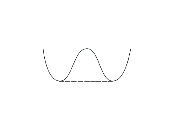
Figure 1: The Double well potential

In perturbation theory, the logarithm diverges where $V_{cl}^{\prime\prime}(\phi)=0,$ while for $V_{cl}^{\prime\prime}(\phi)<0,$ the effective potential becomes complex. The imaginary part is well-known [29] to be related to the decay rate per unit volume for the state of the field. Therefore, such an effective potential, based on the assumption of a stable value of the field, can only be valid for a limited time. Its precise definition therefore requires some care and has been discussed in detail by Weinberg & Wu [20]. The preceding formalism is insufficient, since the exact effective potential is always real and convex [24]. Between the two minima, the true effective potential is expected to look like the dashed line in Fig. 1. The crucial requirement to give meaning to results such as Eq. (12) is that, for some period of time short compared to the decay time, the classical background state is required to be homogeneous. This is a metastable situation which becomes invalid after sufficiently long time. The true ground state for this range of values of the field is described by a breakup into domains within which there are approximately constant but different values of the background. This approximation is even experimentally meaningful in certain situations such as super-cooled steam or super-heated water.

Substantial insight into what happens for small coupling $\lambda$ may be obtained by considering the theory associated with Eq. (7). For small $j>0,$ the potential looks as in Fig. 2.

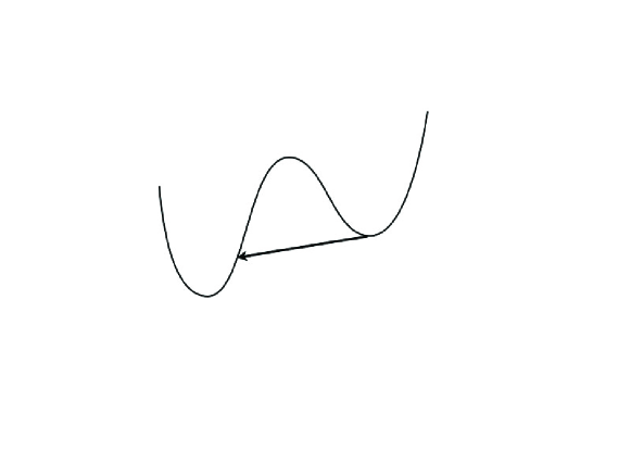
Figure 2: The Double well potential for small $j$.

Classically there are 3 solutions for $\phi_{j}$ to Eq. (8); $U_{j}$ still has two local minima but they are no longer degenerate. The one at $\phi_{j}>0$ is metastable, decaying eventually non-perturbatively via tunnelling. Thus, the effective potential for this homogeneous background acquires a nonperturbative imaginary part. The third solution is a local maximum at a value of $\phi_{j}$ near zero in the perturbatively unstable region $V_{cl}^{{}^{\prime\prime}}<0.$ As a result, the one-loop approximation Eq. (12) has an imaginary part. This instability for long wavelength fluctuations has been discussed in some detail by Guth & Pi [30] and expanded on in Ref. [20]. The breakdown of the homogeneous state is described therein, and we have little to add.

As $j>0$ increases, the metastable minimum approaches the local maximum, and eventually they merge, at which point $U_{j}^{{}^{\prime\prime}}(\phi_{j})=0.$ This is depicted in Fig. 3.

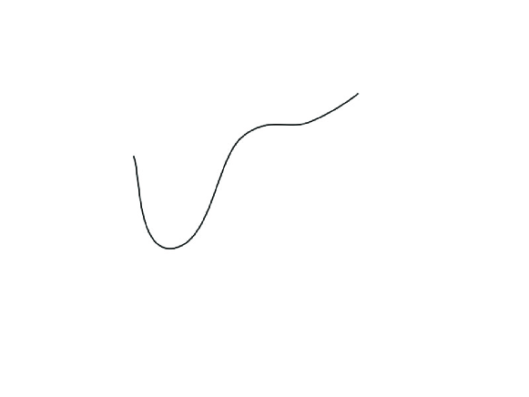
Figure 3: The Double well potential when $U_{j}^{{}^{\prime\prime}}(\phi_{j})=0.$

Since $U_{j}^{{}^{\prime\prime}}=V_{cl}^{{}^{\prime\prime}},$ this is also the point where $M^{2}(\phi)=0.$ To our knowledge, the behaviour of the system at this particular value of $\phi_{j}$ has not been analysed in the literature. Even though the imaginary part of the one-loop effective potential vanishes at this point, it is perturbatively unstable, since, as noted in Ref. [14], the effective potential has power divergences at this point in orders higher than three loops. Specifically, elementary power counting demonstrates that at $L$ loops, $V(\phi)$ includes contributions of the form $\kappa^{3}(\lambda\phi)^{4}\eta^{L-3}$, where

$$\eta=\frac{\kappa\lambda^{2}\phi^{2}}{M^{2}}.$$ (13)

where $\kappa=(16\pi^{2})^{-1}$. This phenomenon does not appear to have been discussed in the literature, presumably because it begins at four loops. It should be no surprise, however, given the situation depicted in Fig. 3. This is an inflection point where fluctuations of one sign do not grow, but fluctuations of opposite sign run away. Given this classical instability, one should not be surprised to find a divergence in perturbation theory. One would expect the growth of perturbations to be less dramatic than in the region of negative curvature. Whereas the correlation length for unstable modes in the regime where $M^{2}(\phi)<0$ is finite, for $M^{2}(\phi)=0$ it is infinite. However, there is a mass scale in the classical potential, viz., $V_{cl}^{{}^{\prime\prime\prime}}(\phi_{j})=\lambda\phi_{j}=\sqrt{2\lambda|m^{2}|}\equiv\Delta,$ and one would expect this to determine the scale of growth of perturbations.

Precisely how these evolve in time has not been determined, but presumably a treatment similar to Ref. [30] should be possible. We have not carried such an analysis, but if, after some time, the system evolves essentially classically, then it is easy to work out the behaviour. For the zero mode, it is clear from the figure that, if the field starts anywhere other than at the inflection point with zero velocity, it will oscillate in time. Regardless of where it is initially, it eventually will roll down the hill, far from the starting point, indicating the instability of small displacements. For short times, one can show that the displacement grows as $t^{2},$ with a coefficient proportional to $\Delta.$ For the quantum mechanical problem, one would have to develop a probability distribution of the displacement similar to Ref. [30].

3 The Yukawa model

Here we consider a simplified model which omits gauge fields; it is also the model used as an introductory example in Ref. [21]. The model resembles the SM in that it displays the phenomenon of vacuum instability for sufficiently large Yukawa coupling, while, as we shall emphasise, differing in some crucial respects. It has the advantage that explicit solutions to the (one-loop) renormalisation group (RG) equations are easily constructed, so the RG evolution is particularly transparent. In this section we will analyse the renormalisation group evolution of the mass and couplings and consider the nature of the theory at different scales, while in the next section we will consider in detail the scalar effective potential.

The model consists of a real scalar field coupled to a set of $n_{F}$ massless Dirac fermions; the Lagrangian is

$$L={\textstyle{\frac{1}{2}}}\partial^{\mu}\phi\partial_{\mu}\phi+i\overline{\psi}_{i}\gamma^{\mu}\partial_{\mu}\psi_{i}-{\textstyle{\frac{1}{2}}}m^{2}\phi^{2}-{\textstyle{\frac{1}{24}}}\lambda\phi^{4}-h\phi\overline{\psi}_{i}\psi_{i}.$$ (14)

In this section we will mainly assume $m^{2}>0$, and make a few comments about the cases $m^{2}<0$ and $m^{2}=0$ at its end; we will return to these cases in more detail in Section 4.

The one-loop $\beta$-functions for the mass $m^{2}$ and the couplings $h$ and $\lambda$ are given by

$$\beta_{m^{2}} = \kappa m^{2}\left(\lambda+4n_{F}h^{2}\right)$$

$$\beta_{\lambda} = \kappa\left(3\lambda^{2}+8n_{F}\lambda h^{2}-48n_{F}h^{4}\right)$$

$$\beta_{h} = (2n_{F}+3)\kappa h^{3},$$ (15)

where $\kappa=(16\pi^{2})^{-1}$. We will also require the scalar anomalous dimension, which at one loop is

$$\gamma_{\phi}=2\kappa n_{F}h^{2}.$$ (16)

To analyse the RG behaviour of the model it is convenient to consider $Y=\lambda/h^{2}$, which satisfies

$$\beta_{Y}=\kappa h^{2}\left(3Y^{2}+(4n_{F}-6)Y-48n_{F}\right),$$ (17)

so that for $n_{F}=1$, $Y$ has fixed points $Y_{+,-}=\frac{1}{3}(1\pm\sqrt{145})\approx 4.35,-3.68$. In Fig. 4, we plot $\beta_{Y}$ against $Y$ for this case.

For all $n_{F}\geq 0$, $Y_{+}>0$ and $Y_{-}<0$; and for large $n_{F}$, $Y_{+,-}\approx 12,-10-4n_{F}/3.$

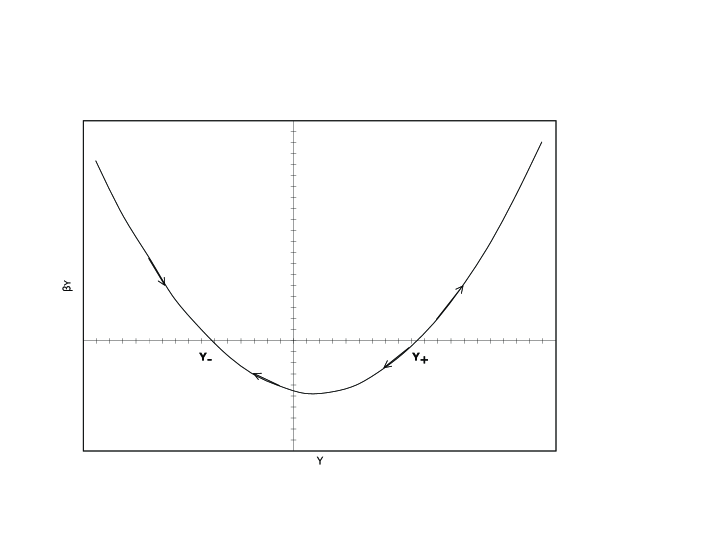
Figure 4: Plot of $\beta_{Y}$ against Y (for $n_{F}=1$). The arrows show the direction of RG flow as $t$ increases.

It is easy to see that $Y_{+,-}$ are IR and UV (ultra-violet) attractive fixed points respectively. Let us consider the evolution of the couplings, starting at $t=\ln\mu=0$; and first look at what happens in the UV, i.e. for $t>0$. The evolution of $h$ is elementary:

$$h^{2}(t)=\frac{h_{0}^{2}}{1-B\kappa h_{0}^{2}t}.$$ (18)

where $B=2(2n_{F}+3)$. As $t$ increases, $h(t)$ approaches a Landau pole, thus evidently departing the perturbatively believable regime. If $Y(0)>Y_{+}$, then $Y(t)$ increases with $t$; eventually $h$ would reach its Landau pole, though in fact, in one-loop approximation, $\lambda$ reaches its Landau pole first. To see this, we require the explicit solution for $Y$ of Eq. (17), which for $Y(0)\equiv Y_{0}>Y_{+}$ is

$$Y(t)=\frac{Y_{+}-z(t)Y_{-}}{1-z(t)}$$ (19)

where

$$z(t)=\frac{Y_{0}-Y_{+}}{Y_{0}-Y_{-}}\left(\frac{h^{2}}{h_{0}^{2}}\right)^{\frac{3(Y_{+}-Y_{-})}{B}}$$ (20)

and we see that $Y\to\infty$ when $z(t)\to 1$, which manifestly occurs for a finite value of $h(t)$.

If $Y_{-}<Y_{0}<Y_{+}$ then it is clear from Eq. (17) that as $t\to\infty$ we will have $Y(t)\to Y_{-}$. Moreover at some finite value of $t$, $t^{\prime}$ say, $Y(t)$ and hence $\lambda(t)$ passes through zero. Clearly the issue of perturbative believability of this result rests simply on the value of $h(t^{\prime})$. The explicit solution for $Y$ in this region is given by

$$Y(t)=\frac{Y_{+}{\overline{z}}(t)+Y_{-}}{1+{\overline{z}}(t)}$$ (21)

where

$${\overline{z}}(t)=\frac{Y_{0}-Y_{-}}{Y_{+}-Y_{0}}\left(\frac{h_{0}^{2}}{h^{2}}\right)^{\frac{3(Y_{+}-Y_{-})}{B}}$$ (22)

so that at $t=t^{\prime}$ we have

$$\frac{h^{2}}{h_{0}^{2}}=\left[\frac{Y_{+}(Y_{0}-Y_{-})}{Y_{-}(Y_{0}-Y_{+})}\right]^{\frac{B}{3(Y_{+}-Y_{-})}}$$ (23)

For $t>t^{\prime}$, $Y\to Y_{-}$; and since $h(t)$ increases with $t$ then so does the magnitude of $\lambda$. Thus the scalar potential becomes negative; and according to the one-loop solution unbounded from below.

Finally for $Y<Y_{-}$, the solution for $Y$ is again given by Eq. (20) and as $t$ increases $Y$ increases towards the fixed point $Y_{-}$.

Now let us discuss what happens in the infra-red, i.e. as $t$ decreases from zero. Let us assume that the scale $\mu_{0}$ corresponding to $t=0$ satisfies $\mu_{0}^{2}>m^{2}$. Since $Y_{+}$ is IR attractive, $Y$ will approach $Y_{+}$ both for $Y_{0}>Y_{+}$ and $Y_{-}<Y_{0}<Y_{+}$, while if $Y_{0}<Y_{-}$, $Y(t)$ decreases as $t$ decreases. The situation changes, however, when $\mu^{2}$ reaches $m^{2}$.

It is well-known that a mass-independent renormalization scheme, such as $\overline{\mbox{\small MS}}$, does not properly take into account threshold effects, so one must be careful extrapolating to scales $\mu^{2}<m^{2}.$ To obtain the correct form of the effective field theory we must integrate out the massive scalar excitations (just as we do not include the top quark contribution to the QCD $\beta$-function in describing physics at scales of a few GeV, for example). The result is a non-renormalisable theory of massless fermions with a series of interactions suppressed by powers of $1/m^{2}.$ One may equally well retain the scalar field as an auxiliary field. In the language of Feynman diagrams, we rewrite each scalar propagator as

$$\frac{1}{p^{2}+m^{2}}=\frac{1}{m^{2}}\cdot\frac{1}{1+p^{2}/m^{2}}.$$ (24)

The factor of $1/(1+p^{2}/m^{2})$ is then expanded as a power series in $p^{2}/m^{2}.$ In this way, the scalar field becomes an auxiliary, i.e., non-propagating, field. To organise the effective field theory, it is useful to associate the factor of $1/m^{2}$ with the vertices at each end of the propagator and the factors of $p^{2}$ with derivatives on the fields. Correspondingly, we rescale $\sigma\equiv m\phi,$ and thus are led to the Lagrangian

$$L=i\overline{\psi}_{i}\gamma^{\mu}\partial_{\mu}\psi_{i}+{\textstyle{\frac{1}{2}}}\sigma^{2}-\frac{h}{m}\sigma\overline{\psi}_{i}\psi_{i}+\frac{\alpha_{1}}{m^{2}}(\partial_{\mu}\sigma)^{2}-\frac{1}{24}\lambda(\frac{\sigma}{m})^{4}-\frac{\alpha_{2}}{m^{4}}(\overline{\psi}\partial_{\mu}\psi)^{2}+\cdots$$ (25)

All terms but the last are just a rewriting of the original Lagrangian, so it appears to be a sleight-of-hand. However, now the “kinetic energy” term (with coefficient $\alpha_{1}$) is to be thought of as a higher-dimensional operator. To leading order, $\alpha_{1}\sim O(h^{2}).$ (Note that $\sigma$ has dimensions of $(\hbox{mass})^{2}$, like an auxiliary field of a supersymmetric theory.) To lowest order in $1/m,$ the auxiliary field is in fact given by

$$\sigma=\frac{h}{m}\overline{\psi}\psi.$$ (26)

It is easy to see from Eq. (25) that the $\sigma^{2}$ term and the Yukawa term are unrenormalised, while the fermion box diagram with four Yukawa insertions gives rise to a $\beta$-function for $\lambda$ of the form

$$\beta_{\lambda}=-48\kappa n_{F}h^{4},$$ (27)

so that

$$\lambda(t)=\lambda(0)-48\kappa n_{F}h^{4}t.$$ (28)

Here we take $t\equiv\ln(\mu/m),$ so that $t<0$ in the low-energy theory. The value of $\lambda(0)$ is obtained by matching to the corresponding coupling in the original theory on scales $\mu>m.$ Moreover, in the expansion in $1/m,$ Eq. (27) and Eq. (28) are exact.

Note that $\lambda$ grows in the IR limit. Now by assumption, $\lambda(0)>0,$ so that the tree vacuum is at $\phi=0$. (Otherwise, the fermions would be massive and the low-energy effective field theory would be different.) Thus the self-interaction of the scalar is repulsive and remains so for all scales in the low-energy theory. Intuitively at least, we would not expect spontaneous symmetry breaking in this regime, a conclusion that will be reinforced by the discussion in the next section.

Let us next consider the case classically scale-invariant case $m^{2}=0$. Let us suppose that, at $t=0,$ we have $Y(0)>Y_{-}$. Then in the IR (since the scalar field does not now decouple), $Y$ flows to the fixed point $Y=Y_{+}$. Since $h\to 0$ in the IR, we therefore have also $\lambda\to 0$. Thus the scalar potential tends to zero smoothly and the origin ($\phi=0$) remains a local minimum of $V(\phi)$.

In the UV, the RG behaviour of the couplings is exactly as in the $m^{2}>0$ case; thus for $Y_{-}<Y(0)<Y_{+}$, $\lambda$ becomes negative, and the potential unbounded from below. As we shall see in the next section, when we consider the radiatively corrected potential, the theory actually undergoes dimensional transmutation[1] leading to interesting structure of the effective potential. Unlike the scalar QED case, the dimensional quantity manifested is in the field value at a maximum of the potential where it turns over. We will consider this case (and the $m^{2}<0$ case) in more detail in the next section.

3.1 The large $n_{F}$ limit

In order to define a weakly-coupled large $n_{F}$ theory we must let $h\to h/\sqrt{n_{F}}$. Then we have for the $\beta$-functions and $\gamma$ the following expressions. For $\mu^{2}>m^{2}$:

$$\beta_{m^{2}} = \kappa m^{2}\left(\lambda+4h^{2}\right)$$

$$\beta_{\lambda} = \kappa\left(3\lambda^{2}+8\lambda h^{2}\right)$$

$$\beta_{h} = 2\kappa h^{3}$$

$$\gamma_{\phi} = 2\kappa h^{2}.$$ (29)

With $Y=\lambda/h^{2}$ once again, we have from Eq. (29)

$$\beta_{Y}=\kappa h^{2}\left(3Y^{2}+4Y\right),$$ (30)

so that in the UV the analysis remains similar, but with points $Y_{+,-}=0,-4/3$.

In the IR limit we see that (due to the rescaling $h\to h/\sqrt{n_{F}}$) we have $\beta_{\lambda}=0,$ so that for $\mu<m,$ the coupling $\lambda$ freezes, remaining constant for $t\to-\infty$.

In the next section we explore the consequences of these RG considerations for the effective potential.

4 The RG improved potential

Ref. [14] contains a detailed analysis of the procedure for RG-improving the effective potential; and in particular the significance of the cosmological constant term $\Omega$ (previously generally neglected) was emphasised. It was also remarked that by considering the renormalisation group improvement of $V^{\prime}\equiv\frac{\partial V}{\partial\phi}$ the $\Omega$-issue may be finessed. Here we will compare the RG improved forms of $V$ and $V^{\prime}$.

We will here use the RG improved forms as follows:

$$V(\mu,\lambda_{i},\phi) = \overline{\xi}(t)^{4}V(\mu(t),\overline{\lambda}_{i}(t),\phi)$$

$$V^{\prime}(\mu,\lambda_{i},\phi) = \overline{\xi}(t)^{4}V^{\prime}(\mu(t),\overline{\lambda}_{i}(t),\phi),$$ (31)

where

$$\frac{d\overline{\lambda}_{i}(t)}{dt} = \overline{\beta}_{i}\left(\overline{\lambda}(t)\right)$$

$$\overline{\beta}_{i} = \frac{\beta_{i}+\delta_{i}\lambda_{i}\gamma}{1+\gamma}$$

$$\overline{\gamma}_{i} = \frac{\gamma}{1+\gamma}$$

$$\overline{\xi}(t) = \exp\left(-\int_{0}^{t}\,\overline{\gamma}\left(\lambda_{i}(t^{\prime})\right)\,dt^{\prime}\right)$$

$$\mu(t) = \mu e^{t}.$$ (32)

Here $\lambda_{i}$ stands for all couplings and masses, with canonical mass dimension $\delta_{i}$ and $\beta_{i}$ is the $\beta$-function for $\lambda_{i}$. Evidently to leading order we have $\overline{\gamma}=\gamma$. The effective potential $V(\phi)$ is given (in the one-loop approximation) as follows:

$$V(\phi) = \Omega(\mu,m,\lambda)+{\textstyle{\frac{1}{2}}}m^{2}\phi^{2}+{\textstyle{\frac{1}{24}}}\lambda\phi^{4}$$ (33)

$$+ \frac{1}{64\pi^{2}}\left[M^{4}\left(\ln\frac{M^{2}}{\mu^{2}}-\frac{3}{2}\right)-4n_{F}h^{4}\phi^{4}\left(\ln\left(\frac{h^{2}\phi^{2}}{\mu^{2}}\right)-\frac{3}{2}\right)\right]$$

where $M^{2}=m^{2}+{\textstyle{\frac{1}{2}}}\lambda\phi^{2}$, and $\Omega$ is the afore-mentioned cosmological constant term (this was denoted $\Omega^{\prime}$ in Ref. [14]).

Our RG improved solutions thus take the form:

$$V(\phi) = \overline{\xi}(t)^{4}\biggl{[}\Omega(t)+{\textstyle{\frac{1}{2}}}m^{2}(t)\phi^{2}+{\textstyle{\frac{1}{24}}}\lambda(t)\phi^{4}+\frac{1}{64\pi^{2}}M^{4}(t)\left(\ln\frac{M^{2}(t)}{\mu^{2}(t)}-\frac{3}{2}\right)$$ (34)

$$- \frac{1}{64\pi^{2}}4n_{F}h^{4}(t)\phi^{4}\left(\ln\frac{h^{2}(t)\phi^{2}}{\mu^{2}(t)}-\frac{3}{2}\right)\biggr{]},$$

$$V^{\prime} = \overline{\xi}(t)^{4}\biggl{[}m^{2}(t)\phi+{\textstyle{\frac{1}{6}}}\lambda(t)\phi^{3}+\frac{1}{32\pi^{2}}\lambda(t)M^{2}(t)\left(\ln\frac{M^{2}(t)}{\mu^{2}(t)}-1\right)$$ (35)

$$- \frac{1}{32\pi^{2}}8n_{F}h^{4}(t)\phi^{3}\left(\ln\frac{h^{2}(t)\phi^{2}}{\mu^{2}(t)}-1\right)\biggr{]}.$$

In order that $V$ satisfy the usual RG equation, $\Omega(\mu,\lambda_{i})$ must itself satisfy an RG equation which to leading order can be written

$$\left[\mu\frac{\partial}{\partial\mu}+\beta_{i}\frac{\partial}{\partial\lambda_{i}}\right]\Omega=\frac{1}{32\pi^{2}}m^{4}.$$ (36)

In Ref. [32] and Ref. [14] the consequences of various choices for $\Omega$ were considered. For example, one may decide to require that $\Omega$ be free of explicit dependence on $\mu$; in the absence of the Yukawa coupling $h$ the resulting solution of Eq. (36) (using one-loop $\beta$-functions) is

$$\Omega=-m^{4}\left(\frac{1}{2\lambda}+\frac{c}{\lambda^{\frac{2}{3}}}\right),$$ (37)

where $c$ is an arbitrary constant. It is interesting that when we renormalisation improve the solution as described above, the $c$-term in Eq. (37) remains independent of $t$ in this case because we have

$$\lambda(t) = \frac{\lambda_{0}}{1-3\kappa\lambda_{0}t}$$

$$m^{2}(t) = \frac{m^{2}(0)}{(1-3\kappa\lambda_{0}t)^{\frac{1}{3}}}.$$ (38)

The case $h\neq 0$ is not so easy to analyse.

A more natural form for $\Omega$ is

$$\Omega=-\hat{V}(\phi)\Bigm{|}_{\phi=v}$$ (39)

where $\hat{V}(\phi)$ is the potential omitting $\Omega$, and $v$ is the value of $\phi$ at any extremum of $\hat{V}$. Of course the simplest such extremum is $v=0$, corresponding to a solution for $\Omega$ which is (to leading order)

$$\Omega=-\frac{1}{64\pi^{2}}m^{4}\ln\frac{m^{2}}{\mu^{2}}.$$ (40)

This corresponds of course to simply subtracting the value of $V$ at $\phi=0$. It is this form of $\Omega$ we use in the subsequent analysis.

Let us now consider the behaviour of the potential as a function of $\phi$. We will consider separately the three cases $m^{2}>0$, $m^{2}=0$ and $m^{2}<0$.

4.1 The $m^{2}>0$ case

For $\phi\to 0$, if we choose $t$ so that $\mu(t)=\phi,$ then this controls the logarithm in the fermion loop contribution; the scalar loop contribution decouples for $\mu^{2}<m^{2}$ (as described in the last section for the $\beta$-functions) and must hence be removed from Eqs. (34,35)  and we replace Eq. (40)  by $\Omega=0$. The behaviour of the potential for $\phi^{2}<m^{2}$ is then determined by the IR RG evolution of $\lambda$ which we explored in the last section, culminating in Eq. (28). From this it is clear that, with $\mu\sim\phi$, $\lambda$ grows like $\lambda\sim-\ln\phi$, and hence $V\sim m^{2}\phi^{2}/2+\lambda\phi^{4}/24\to 0$.

The question to be addressed now is whether we can conclude that this represents the ground state of the theory; so let us examine the potential for large $\phi$. Once again we choose $t$ so that $\mu=\phi$, in order to control the logarithms in Eqs. (34,35). Note that Eq. (40) contains a potentially large logarithm, but at large $\phi$, $\Omega$, being of $O(m^{4})$, is negligible in any event. We will explicitly verify this presently. So the behaviour is controlled by the UV evolution of the couplings.

Let us first consider $Y(0)>Y_{+}$. In that case, as described in the last section both $h$ and $\lambda$ increase until $\lambda$ reaches a Landau pole. Before this the theory of course becomes non-perturbative; the potential is never lower than it is at the origin while perturbation theory remains reliable. If we invoke a UV cut-off $\Lambda$ representing the scale of new physics then the theory may or may not remain perturbative up to the cut-off. In either event, we conclude that it is possible that $\phi=0$ represents the ground state of the theory; we cannot be certain either because of the non-perturbative nature of the theory in the UV, or because of the new physics beyond the cut-off.

Now consider the case $Y_{-}<Y_{0}<Y_{+}$. Now as $t$ increases $Y$ flows towards the fixed point at $Y=Y_{-}$. Thus $\lambda$ and eventually $V$ become negative; depending on the initial conditions this can certainly happen for perturbative values of the couplings $h,\lambda$. As mentioned above, just how far one can proceed toward the IR using these $\beta$-functions depends on the value of $m^{2},$ since these assume that $m^{2}$ is sufficiently small so that the scalar particle has not decoupled.

As an illustration, in Fig. 5 we plot $V(\phi)$ (rather, $V(t)$) as calculated from Eq. (34) and from integrating Eq. (35) for $n_{F}=1$ and values (at $t=0$) $\lambda=h=1$ and $\mu=m^{2}$, normalising so that at $t=0$, $V=0$. We denote the results for $V$ from the two calculations as $V_{a}$ and $V_{b},$ respectively. The results for $V_{a}$ and $V_{b}$ are not precisely the same; the fact that they agree well for the range of $t$ displayed is because we are still in the perturbative regime. We see clearly that at $t=t^{*}\approx 3.6,$ the potential passes through zero becomes rapidly negative. (Note that the potential inevitably passes through an extremum (a maximum) before becoming negative; we will analyse this extremum in more detail in the special case $m^{2}=0,$ which we will consider presently.) Evidently we are inclined to deduce that the tree minimum at $\phi=0$ is not the ground state of the theory. Can we trust this conclusion? First, note that, with our initial conditions, we have $h(t^{*})\approx 1.14$ which is manifestly still perturbative.

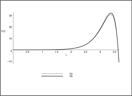
Figure 5: Plot of $V_{a}$ and $V_{b}$ against $t=\ln\mu$

We must also require that the cut-off $\Lambda$ representing the scale of new physics satisfies $\ln\Lambda>t^{*}$, if we are to trust the calculation of $V(t^{*})$. (Of course for values of $\phi$ close to the cut-off we would have to consider the effect of higher dimensional operators suppressed by one or more power of the cut-off [33]-[36]. Here we agree with Ref. [35] that the effect of such operators on instability bounds is necessarily small whenever it can be reliably calculated.) Now for fixed $h(0)$, as we increase $\lambda(0)$ (and hence $Y(0)$), $t^{*}$ increases. Thus for a given cut-off $\Lambda$, the value of $\lambda(0)$ such that $e^{t^{*}}=\Lambda$ is the upper limit on $\lambda(0)$ corresponding to a theory such that we can conclude that the potential becomes negative. A separate issue is that for sufficiently large $t$, $h(t)$ becomes large and we can no longer trust our calculation. For $e^{t^{*}}<\Lambda$, therefore, we cannot necessarily deduce that the theory has no ground state; but we claim we can conclude that the ground state (if it exists) is lower than the tree minimum.

Note that $V$ passes through zero at $t\approx 3.6$. With the same initial conditions, the coupling $\lambda$ passes through zero at $t=t^{\prime}\approx 2.97$, and $M^{2}$ passes through zero at $t\approx 2.98$. Therefore for $t>2.98$ the potential (including one loop corrections) in fact has an explicit perturbative imaginary part; in Fig. 5 we have taken the real part of the potential. This imaginary part is similar to that which develops in $\phi^{4}$-theory for $m^{2}<0$ as $\phi$ is reduced.

Now at $M^{2}<0$ we have argued above that the imaginary part of the potential has a straightforward interpretation. Let us consider the potential precisely at the value of $\phi$ defined by $M^{2}=0$. Beginning at $L=4$, the potential contains power singularities at $M^{2}=0$, as explained in section 2 in the context of the pure scalar theory. (Note that in the $m^{2}<0$ case, $M^{2}=0$ occurs at a positive value of $\lambda$, and so happens at both a large value of $\phi$ (as $\lambda$ approaches zero) and a small value.) Reverting to the $m^{2}>0$ case we have been discussing, we must conclude that the perturbation expansion for $V$ breaks down for values of $t$ such that $M^{2}\approx 0$. In Fig. 5 this corresponds to $t\approx 2.98$, as we have already mentioned. However, at $t^{*}\approx 3.6$, where $V$ passes through zero, we find that $\eta\approx-0.004$; the range of $\phi$ for which $\eta>1$ (and hence for which $V$ cannot be reliably calculated in perturbation theory) is very small indeed.

The arguments presented in Ref. [21] amount essentially to the statement that the region of validity of $V(\phi)$ is curtailed by the requirement that $\lambda(\Lambda)>0$; and they propose that the region of validity of $V(\phi)$ be defined by the inflection point in the potential (if this occurs a scale below $\Lambda$), which we see from Fig. 5 indeed occurs at the point where $\lambda$ changes sign as described above. They further conclude that this model does not exhibit the vacuum instability described above; for $m^{2}>0$ the ground state of the theory is at $\phi=0$, and the potential is a convex function within its region of validity (simply because this region is curtailed at the inflection point. We simply disagree with this analysis; as we have described above, the work of Refs. [20] and [30] demonstrate quite convincingly, in our opinion, that the potential has meaning in its non-convex region; and we see no reason to require that $\lambda(\Lambda)>0$. As usual, we need to require, for perturbative believability, that relevant expansion parameters are “sufficiently” small; and in our examples, since we use renormalisation group-improved perturbation theory, at large $\phi$ these parameters are simply the dimensionless couplings evaluated at a scale commensurate with $\phi$ in the UV region. It seems clear to us, therefore, that for the choice of parameters used in Fig. 5, we can certainly conclude that the local minimum $\phi=0$ is unstable.

It is essentially for the same reason that we disagree with Refs. [22], [23]. There the claim is that the calculation of the potential in a theory without a UV cut-off disagrees with same calculation with a cut-off and that the latter agrees with simulation data. We claim, however, that the exhibition of this disagreement occurs invariably in regions of parameter space where perturbation theory is not to be trusted. When there is substantial disagreement between the theory with and without a cutoff, it is a sure sign that the scale of the field is not far below the scale of the cutoff. Perturbation theory breaks down because either $h$ or $\lambda$ become large. This has, therefore, no bearing on our discussion above, where we are always careful to confine our conclusions to regions of parameter space where perturbation theory is expected to remain valid.

4.2 The $m^{2}=0$ case

We turn now to the interesting case when $m^{2}=0$. The analysis of this can be done with the full RG apparatus developed above, but it is both interesting and illuminating to mimic the original simplified CW treatment of scalar QED. Let us suppose for simplicity that $0<Y(0)<Y_{+}$. For this range we have seen in section 2 that $\lambda$ approaches zero as $t$ increases. For $\lambda(t)$ sufficiently small, we may neglect the higher-order corrections in $\lambda,$ so the effective potential may be written as

$$V_{eff}=\phi^{4}\left[\frac{\lambda}{4!}-n_{F}\frac{h^{4}}{16\pi^{2}}\ln(\phi^{2}/v^{2})\right],$$ (41)

where the scale $v$ will be defined presently. Then

$$V^{\prime}_{eff}=\phi^{3}\left[\frac{\lambda}{3!}-n_{F}\frac{h^{4}}{8\pi^{2}}\left(1+2\ln(\phi^{2}/v^{2})\right)\right].$$ (42)

Evidently $V^{\prime}_{eff}$ vanishes for a nonzero value of $\phi$ as well as at the origin. If we choose the scale $v$ to be the value of $\phi$ at this extremum, then we find it occurs at the scale where the running couplings satisfy the relation

$$\lambda=n_{F}\frac{3h^{4}}{4\pi^{2}},$$ (43)

at which point

$$V^{\prime\prime}_{eff}=-n_{F}\frac{h^{4}}{2\pi^{2}}\ v^{2}<0.$$ (44)

Thus there is a maximum value defined by dimensional transmutation, beyond which the potential steadily decreases. This discussion is very similar to the CW one for scalar QED, except that there, because the $e^{4}$ contribution to the effective potential differs in sign from the $h^{4}$ one, the extremum is a minimum, and Eq. (43) above is replaced by the equation $\lambda=-9\kappa e^{4}$.

Returning to the case $m^{2}>0,$ it should now be clear that the preceding analysis will remain valid to a good approximation so long as $m^{2}<<v^{2}$, as in fact is the case for the values we chose to produce Fig. 5. In fact, at the maximum of $V$ displayed in Fig. 5, we find that $\lambda\sim-0.2$ while $h\sim 1.12$. Note that $\lambda$ and $h^{4}/(4\pi^{2})$ are indeed of the same order of magnitude at the maximum, as we would expect.

In a derivation based on the RG-improved form of the potential (Eq. (34) or its derivative Eq. (35)) Eq. (43) is replaced by the equation [37, 38]

$$4\lambda+\beta_{\lambda}=0,$$ (45)

but the essential features of the calculation are unaffected. We might note that the Yukawa model is more amenable to perturbative treatment than scalar QED. In the latter case, while the existence of a local minimum could be unambiguously demonstrated perturbatively, the behaviour of the potential both in a neighborhood of the origin as well as for large field values was beyond the realm of perturbation theory. In our case, we are able to treat both the origin and the maximum perturbatively, with the breakdown of perturbation theory restricted to large values of the field.

The only caveat on this discussion is that the coupling $h(v)$ be sufficiently small so that it is in the perturbative regime. According to our discussion in the previous section, there is then always a scale $\lambda$ at which the relation (43) holds. To conclude, in the case $m^{2}=0,$ the origin is metastable and decays to a region where eventually the couplings are strong. Once again, whether the theory has no ground state or is replaced at high scales by a modified theory cannot be determined within this framework. There is hardly a more compelling application of radiative corrections than dimensional transmutation, yet it is completely missed by the arguments of ref. [21] and overlooked in lattice results, ref. [22, 23], whose range of mass parameters does not include this important region.

4.3 The $m^{2}<0$ case

Finally, we consider the case $m^{2}<0.$ At the classical level, the scalar field behaves as in the case of the $\phi^{4}$ model discussed in section 2.1, i.e., the potential has minima at $\phi=\pm v,$ where

$$v^{2}=\frac{-6m^{2}}{\lambda}.$$ (46)

The theory undergoes spontaneous symmetry breaking, and the scalar gets a mass $m_{H}$ with $m_{H}^{2}=-2m^{2}=\lambda v^{2}/3.$ As a result, each fermion also gets a mass $m_{f}=hv.$ The ratio of the masses is

$$\frac{m_{H}^{2}}{m_{f}^{2}}=\frac{\lambda}{3h^{2}}=\frac{Y}{3}.$$ (47)

Radiative corrections to this classical behaviour will shift the values of the minima and the masses, but so long as perturbation theory holds, this qualitative behaviour is unchanged. The remainder of the discussion can be inferred from the behaviour of the running couplings. Generically, $Y\sim O(1).$ The behaviour for large field values leads us to choose the scale $\mu$ to be $O(\phi)$ to avoid large logs; and the UV behaviour of $Y(\mu)$ has been discussed in detail in section 2. For small values of the field, however the potential is not given correctly by choosing $\mu\sim\phi.$ When the field is small compared to the masses of the scalar and the fermions, they both decouple. The theory in the infrared is just that of a set of $n_{F}$ massive free fermions and a massive free scalar, so the running of the couplings below these masses is not correctly given by a mass-independent renormalization scheme.

5 The Standard Model

The study of the possible SM vacuum instability has a long history and a substantial literature. The first comprehensive treatment from an RG perspective was in Ref. [14]; subsequent refinements included a particularly lucid discussion in Ref. [18]). The situation in the SM is similar to the Yukawa model we have considered, in that the one loop fermion contribution to $V$ potentially destabilises the electro-weak vacuum; however it differs in that onset of the instability is associated with another, deeper, minimum of the potential (which may still occur within the perturbative regime).

The deeper minimum can occur because while the top quark Yukawa coupling contribution to the evolution of the Higgs self-coupling $\lambda$ evolution tends to push it down towards (or through) zero in the UV, the Yukawa coupling itself gets smaller in the UV due to the gauge coupling contributions to its evolution. Therefore eventually the gauge coupling contributions to the evolution of $\lambda$ cause it to recover to positive values. It is easy to verify this from the explicit expressions for the $\beta$-functions [3], which for convenience we reproduce below. (Note that the scalar anomalous dimension is gauge dependent: the result below is for the Landau gauge.)

The one-loop RG functions are

$$\kappa^{-1}\gamma^{(1)} = 3h^{2}-{\textstyle{\frac{9}{4}}}g^{2}-{\textstyle{\frac{3}{4}}}{g^{\prime}}^{2}$$

$$\kappa^{-1}\beta_{\lambda}^{(1)} = 4\lambda^{2}+12\lambda h^{2}-36h^{4}-9\lambda g^{2}-3\lambda{g^{\prime}}^{2}$$

$$+ {\textstyle{\frac{9}{4}}}{g^{\prime}}^{4}+{\textstyle{\frac{9}{2}}}g^{2}{g^{\prime}}^{2}+{\textstyle{\frac{27}{4}}}g^{4}$$

$$\kappa^{-1}\beta_{h}^{(1)} = {\textstyle{\frac{9}{2}}}h^{3}-8g_{3}^{2}h-{\textstyle{\frac{9}{4}}}g^{2}h-{\textstyle{\frac{17}{12}}}{g^{\prime}}^{2}h$$

$$\kappa^{-1}\beta_{g}^{(1)} = -{\textstyle{\frac{19}{6}}}g^{3}$$

$$\kappa^{-1}\beta_{g^{\prime}}^{(1)} = {\textstyle{\frac{41}{6}}}{g^{\prime}}^{3}$$

$$\kappa^{-1}\beta_{g_{3}}^{(1)} = -7g_{3}^{3}$$

$$\kappa^{-1}\beta_{m^{2}}^{(1)} = m^{2}(2\lambda+6h^{2}-{\textstyle{\frac{9}{2}}}g^{2}-{\textstyle{\frac{3}{2}}}{g^{\prime}}^{2}).$$ (48)

The two-loop contributions to the RG functions are given by [3]

$$\kappa^{-2}\gamma^{(2)} = {\textstyle{\frac{1}{6}}}\lambda^{2}-{\textstyle{\frac{27}{4}}}h^{4}+20g_{3}^{2}h^{2}+{\textstyle{\frac{45}{8}}}g^{2}h^{2}+{\textstyle{\frac{85}{24}}}{g^{\prime}}^{2}h^{2}$$

$$- {\textstyle{\frac{271}{32}}}g^{4}+{\textstyle{\frac{9}{16}}}g^{2}{g^{\prime}}^{2}+{\textstyle{\frac{431}{96}}}{g^{\prime}}^{4}$$

$$\kappa^{-2}\beta_{\lambda}^{(2)} = -{\textstyle{\frac{26}{3}}}\lambda^{3}-24\lambda^{2}h^{2}+6\lambda^{2}(3g^{2}+{g^{\prime}}^{2})-3\lambda h^{4}+80\lambda g_{3}^{2}h^{2}$$

$$+ {\textstyle{\frac{45}{2}}}\lambda g^{2}h^{2}+{\textstyle{\frac{85}{6}}}\lambda{g^{\prime}}^{2}h^{2}-{\textstyle{\frac{73}{8}}}\lambda g^{4}+{\textstyle{\frac{39}{4}}}\lambda g^{2}{g^{\prime}}^{2}+{\textstyle{\frac{629}{24}}}\lambda{g^{\prime}}^{4}$$

$$+ 180h^{6}-192h^{4}g_{3}^{2}-16h^{4}{g^{\prime}}^{2}-{\textstyle{\frac{27}{2}}}h^{2}g^{4}+63h^{2}g^{2}{g^{\prime}}^{2}$$

$$- {\textstyle{\frac{57}{2}}}h^{2}{g^{\prime}}^{4}+{\textstyle{\frac{915}{8}}}g^{6}-{\textstyle{\frac{289}{8}}}g^{4}{g^{\prime}}^{2}-{\textstyle{\frac{559}{8}}}g^{2}{g^{\prime}}^{4}-{\textstyle{\frac{379}{8}}}{g^{\prime}}^{6}$$

$$\kappa^{-2}\beta_{h}^{(2)} = h\bigl{(}-12h^{4}+h^{2}({\textstyle{\frac{131}{16}}}{g^{\prime}}^{2}+{\textstyle{\frac{225}{16}}}g^{2}+36g_{3}^{2}-2\lambda)+{\textstyle{\frac{1187}{216}}}{g^{\prime}}^{4}$$

$$- {\textstyle{\frac{3}{4}}}g^{2}{g^{\prime}}^{2}+{\textstyle{\frac{19}{9}}}{g^{\prime}}^{2}g_{3}^{2}-{\textstyle{\frac{23}{4}}}g^{4}+9g^{2}g_{3}^{2}-108g_{3}^{4}+{\textstyle{\frac{1}{6}}}\lambda^{2}\bigr{)}$$

$$\kappa^{-2}\beta_{g}^{(2)} = g^{3}({\textstyle{\frac{3}{2}}}{g^{\prime}}^{2}+{\textstyle{\frac{35}{6}}}g^{2}+12g_{3}^{2}-{\textstyle{\frac{3}{2}}}h^{2})$$

$$\kappa^{-2}\beta_{g^{\prime}}^{(2)} = {g^{\prime}}^{3}({\textstyle{\frac{199}{18}}}{g^{\prime}}^{2}+{\textstyle{\frac{9}{2}}}g^{2}+{\textstyle{\frac{44}{3}}}g_{3}^{2}-{\textstyle{\frac{17}{6}}}h^{2})$$

$$\kappa^{-2}\beta_{g_{3}}^{(2)} = g^{3}_{3}({\textstyle{\frac{11}{6}}}{g^{\prime}}^{2}+{\textstyle{\frac{9}{2}}}g^{2}-26g_{3}^{2}-2h^{2})$$

$$\kappa^{-2}\beta_{m^{2}}^{(2)} = 2m^{2}\bigl{(}-{\textstyle{\frac{5}{6}}}\lambda^{2}-6\lambda h^{2}+2\lambda(3g^{2}+{g^{\prime}}^{2})-{\textstyle{\frac{27}{4}}}h^{4}+20g_{3}^{2}h^{2}$$ (49)

$$+ {\textstyle{\frac{45}{8}}}g^{2}h^{2}+{\textstyle{\frac{85}{24}}}{g^{\prime}}^{2}h^{2}-{\textstyle{\frac{145}{32}}}g^{4}+{\textstyle{\frac{15}{16}}}g^{2}{g^{\prime}}^{2}+{\textstyle{\frac{157}{96}}}{g^{\prime}}^{4}\bigl{)}.$$

Here $h,\lambda$ are the Yukawa and Higgs self-coupling normalised so that $m_{t}=hv/\sqrt{2}$ and $\lambda=6m^{2}/v^{2}=3m_{h}^{2}/m^{2}$ where $v\sim 246$ GeV.

One easily sees that for a given $h$, there will be a lower limit on $\lambda$ such that the electroweak vacuum is the true one; this corresponds (for a given $m_{t}$) to a lower bound on the Higgs mass $m_{h}$.

For $m_{h}$ below this bound the electroweak vacuum would be metastable. Here we have little to add to the discussion of Ref. [18]. For a cut-off $\Lambda=1~{}\hbox{TeV},$ the bound is about [18]

$$m_{H}(\hbox{GeV})>52+0.64(m_{t}(\hbox{GeV})-175)-0.5\frac{\alpha(M_{Z})-0.118}{0.006},$$ (50)

leaving us with comforting stability, given existing experimental knowledge of $m_{t}$ and bounds on $m_{h}$. For $\Lambda=10^{19}~{}\hbox{GeV}$, the bound $m_{H}(\hbox{GeV})>52~{}\hbox{GeV}$ above becomes $m_{H}(\hbox{GeV})>134~{}\hbox{GeV}$, so it remains possible that the discovery of a Higgs (with $m_{H}(\hbox{GeV})<134~{}\hbox{GeV}$) will provide, from this point of view, evidence for physics beyond the standard model.

The $M^{2}=0$ instability on which we remarked occurs in this case too, and is similarly confined to a very narrow range of $\phi$ values well away from the value of $\phi$ at which the potential drops below the electro-weak minimum.

The SM analysis is repeated in Ref. [21] where their philosophy that the physical cut-off may not be higher than the inflection point in the potential leads, (for smaller values of the cut-off) to substantially different lower bounds on $m_{H}$ than those obtained in Ref. [18]. They also assert that the metastable scenario described above cannot occur, due essentially to the convex nature of the potential. We maintain that is not correct, as we have explained above.

6 Conclusions

Using mainly the simple $\lambda\phi^{4}$ theory and its extension involving Yukawa couplings, we have reviewed aspects of the computation of the scalar effective potential that are sensitive to non-convex regions of the potential, with a particular focus on the issue of ground state stability. We have found no reason to disbelieve that a sufficiently large fermionic contribution will destabilise the tree vacuum (corresponding to the origin in a simple theory with scalar $m^{2}\geq 0$ or to the electroweak vacuum in the SM.) Moreover this instability can be consistently demonstrated within the confines of perturbative believability. The Yukawa model we have studied has the additional interesting feature that it exhibits weak-coupling dimensional transmutation associated with a local maximum of the potential. The scale associated with dimensional transmutation is crucial, since it sets the value of the field where the instability may occur, even when $m^{2}\neq 0.$

We conclude that calculations of the effective potential within the perturbative domain can be trusted, and inferences about metastability relied upon. While the ultimate effective potential may be convex, or the constrained effective potential rather different from the perturbative calculation, their application are not in contradiction with this conclusion. One simply must be careful about the questions one wishes to address. The formalism employed must conform to the particular physical situation under discussion.

References

- [1] S. Coleman and E. Weinberg, Phys. Rev. D7 (1973) 1888.
- [2] R. Jackiw, Phys. Rev. D9 (1974) 1686.
- [3] C. Ford, I. Jack and D. R. T. Jones, Nucl. Phys. B387 (1992) 373, [Erratum-ibid. B504 (1997) 551].
- [4] S. P. Martin, Phys. Rev. D 66 (2002) 096001.
- [5] D. Boyanovsky, H. J. de Vega and D. J. Schwarz, arXiv:hep-ph/0602002.
- [6] M. Quiros, arXiv:hep-ph/9901312.
- [7] E. W. Kolb, M. Abney, E. J. Copeland, A. R. Liddle and J. E. Lidsey, arXiv:astro-ph/9407021.
- [8] P. Q. Hung, Phys. Rev. Lett. 42 (1979) 873.
- [9] N. Cabibbo, L. Maiani, G. Parisi and R. Petronzio, Nucl. Phys. B158 (1979) 295.
- [10] R.A. Flores and M. Sher, Phys. Rev. D27 (1983) 1679.
- [11] M. Lindner, Z. Phys. 31 (1986) 295.
- [12] M. Sher, Phys. Rep. 179 (1989) 273.
- [13] M. Lindner, M. Sher and H. W. Zaglauer, Phys. Lett. B228 (1989) 139.
- [14] C. Ford, D.R.T. Jones, P.W. Stephenson and M.B. Einhorn, Nucl. Phys. B395 (1993) 17.
- [15] M. Sher, Phys. Lett. B317 (1993) 159.
- [16] G. Altarelli and G. Isidori, Phys. Lett. B337 (1994) 141.
- [17] J.A. Casas, J.R. Espinosa and M. Quirós, Phys. Lett. B342 (1995) 171.
- [18] J.A. Casas, J.R. Espinosa and M. Quirós, Phys. Lett. B382 (1996) 374.
- [19] G. Isidori, G. Ridolfi and A. Strumia, Nucl. Phys. B609 (2001) 387.
- [20] E. J. Weinberg and A. Wu, Phys. Rev. D36 (1987) 2474.
- [21] V. Branchina and H. Faivre, Phys. Rev. D72 (2005) 065017.
- [22] K. Holland, J. Kuti, Nucl. Phys. Proc. Suppl. 129 (2004) 765.
- [23] K. Holland, arXiv:hep-lat/0409112.
- [24] J. Iliopoulos, C. Itzykson and A. Martin, Rev. Mod. Phys. 47 (1975) 165.
- [25] M. Luscher and P. Weisz, Phys. Lett. B 212, 472 (1988).
- [26] M. Luscher and P. Weisz, Nucl. Phys. B 290, 25 (1987); ibid. 295, 65 (1988).
- [27] C. B. Lang, Nucl. Phys. B 265, 630 (1986).
- [28] D. J. E. Callaway, Phys. Rept. 167, 241 (1988).
- [29] S. Coleman, Aspects of symmetry: selected Erice lectures of Sidney Coleman. Cambridge: Cambridge Univ. Press, 1985.
- [30] A. H. Guth and S. Y. Pi, Phys. Rev. D32 (1985) 1899.
- [31] M. B. Einhorn and J. Wudka, JHEP 0108 (2001) 025.
- [32] B. M. Kastening, Phys. Lett. B283 (1992) 287.
- [33] A. Datta, B. L. Young and X. Zhang, Phys. Lett. B385 (1996) 225.
- [34] B. Grzadkowski, J. Pliszka and J. Wudka, Phys. Rev. D69 (2004) 033001.
- [35] C. P. Burgess, V. Di Clemente and J. R. Espinosa, JHEP 0201 (2002) 041.
- [36] B. Grzadkowski, J. Pliszka and J. Wudka, Phys. Rev. D69 (2004) 033001.
- [37] H Yamagishi, Nucl. Phys. B216 (1983) 508.
- [38] M.B. Einhorn and D.R.T. Jones, B211 (1983) 29.
- [39] C.T. Hill, Phys. Rev. D24 (1981) 691.