Abstract

The observed light neutrinos may be related to the existence of new heavy neutrinos in the spectrum of the SM. If a pair of heavy neutrinos has nearly degenerate masses, then CP violation from the interference between tree-level and self-energy graphs can be resonantly enhanced. We explore the possibility of observing CP asymmetries due to this mechanism at the LHC. We consider a pair of heavy neutrinos $N_{1,2}$ with masses ranging from $100-500\,{\rm GeV}$ and a mass-splitting $\Delta m_{N}=m_{N_{2}}-m_{N_{1}}$ comparable to their widths $\Gamma_{N_{1,2}}$. We find that for $\Delta m_{N}\sim\Gamma_{N_{1,2}}$, the resulting CP asymmetries can be very large or even maximal and therefore, could potentially be observed at the LHC.

1 Introduction

The observation of neutrino oscillations has established that the observed neutrinos are not massless and so the Standard Model (SM) must be extended in order to accommodate these [1]. In order to explain why the neutrinos are so much lighter than any of the other fermions, it is common to postulate that in addition to the three observed light neutrinos, there also exist partner heavy neutrinos. In order to avoid very stringent constraints due to their non-observation at the Large Electron–Positron (LEP) collider, these must have masses greater than about $100\,{\rm GeV}$ [6]. However, if they exist with masses greater than this, but less than about $500\,{\rm GeV}$, they fall into the category of particles that could be produced for the first time at the Large Hadron Collider (LHC) [7, 8, 11, 12]. Complementary to such a search, heavy neutrinos could also be observed at a future linear collider. Several studies have been conducted into their signals at the International Linear Collider (ILC) [13, 16] as well as possible alternatives such as an $e^{-}\gamma$ collider [17].

If neutrinos with such masses do exist, then in general they should break lepton-flavour conservation and, if they are Majorana, lepton-number ($L$) conservation as well. Furthermore, since their couplings can be complex, they can also contribute to CP violation. A scenario of particular interest is if two or more of the heavy neutrinos are quasi-degenerate in mass [19]. In this case, CP violation can be resonantly enhanced such that for appropriate couplings, CP asymmetries can be large or even maximal [22]. By introducing flavour symmetries in the singlet neutrino sector, models can be built where quasi-degenerate heavy neutrinos with masses of order the electroweak scale appear naturally [23]. These mostly focus on models of resonant leptogenesis, which can be used to explain the Baryon Asymmetry of the Universe (BAU). Observation of heavy neutrinos at the LHC, and in particular, measurements of CP asymmetries due to them would be a way of testing such models.

Since it is not known at this time whether neutrinos are Dirac or Majorana particles, both possibilities need to be considered. For the former, the collider signatures at the LHC are lepton-flavour-violating (LFV) processes. For the latter, in addition to these, lepton-number-violating (LNV) processes could also be observed. Either of these types of processes should be virtually background free since they are forbidden in the SM which is both lepton-number-conserving (LNC) and lepton-flavour-conserving (LFC). Higher order processes with light neutrinos in the final state could in principle fake the signals, but these can be excluded by suitable kinematical cuts, e.g., by vetoing on missing transverse momentum ($p_{T}$) cut [11, 12].

CP violation could show up in asymmetries between possible signal final states and their CP-conjugates. Although the initial $pp$ state is not a CP-eigenstate, true CP-violating observables can be constructed, either by taking into account the theoretically calculable difference expected due to the Parton Distribution Functions (PDF’s) [27, 28], or by considering appropriate ratios of different processes such that this factor drops out.

Observation of heavy neutrinos at the LHC would be a major discovery. Less direct evidence could come from them contributing to LFV decays, e.g. $\mu\to e\gamma$, $\mu\to e$ conversion in nuclei, or (if Majorana) neutrinoless double beta decay. The non-observation of such processes, along with the excellent agreement of electroweak data to the SM, places limits on the strength of their couplings.

This paper is organised as follows: In Section 2, we describe extensions of the SM which include heavy neutrinos and discuss the experimental constraints on them. Two specific models are considered, one predicting heavy Majorana neutrinos, the other Dirac. Section 3 is a short discussion of the signatures of such particles at the LHC, in particular, we classify them according to whether or not they are LNV. Next, in Section 4, we present the formalism for describing the propagator of a system of two coupled quasi-degenerate heavy neutrinos. This is based on the field-theoretic resummation approached developed in [29] for describing resonant transitions involving the mixing of intermediate fermionic states.

Assuming the signals are due entirely to two nearly degenerate heavy (Dirac or Majorana) neutrinos, the $2\times 2$ propagator matrices for such a pair are then used in Section 5 to derive expressions for the CP asymmetries between them. We give example scenarios where these asymmetries are large and discuss their compatibility with both experimental and theoretical constraints. In Section 6, we use these scenarios in order to produce numerical estimates of the possible level of leptonic CP violation observable at the LHC. We define a number of CP-violating observables and plot these, along with the cross sections they are derived from. Finally, Section 7 contains our conclusions.

2 Heavy Neutrino Extensions of the Standard Model

2.1 Heavy Majorana Neutrino Model

We first describe the SM, minimally extended to include right-handed neutrinos. Assuming the Higgs sector is not extended, the Lagrangian describing the neutrino masses and mixings reads

$$\mathcal{L}_{m_{\nu}}=-\frac{1}{2}\left(\begin{array}[]{cc}\overline{\nu_{L}^{0}}&\overline{{(\nu_{R}^{0})}^{c}}\end{array}\right)\left(\begin{array}[]{cc}0&m_{D}\\ m_{D}^{T}&m_{M}\end{array}\right)\left(\begin{array}[]{c}{(\nu_{L}^{0})}^{c}\\ \nu_{R}^{0}\end{array}\right)+{\rm h.c.},$$ (2.1)

where $\nu_{L}^{0}$ and $\nu_{R}^{0}$ denote column vectors of the left- and right-handed neutrino fields in the weak basis, and the notation $\nu^{c}\equiv C\overline{\nu}^{T}$ represents the charge conjugate fields. Although it is commonly assumed that there is one right-handed neutrino per generation (as required in $SO(10)$ Grand Unified Theories (GUT’s) [30]), this needs not be so in the bottom up approach considered here. In fact, as will be shown in Section 5, in the context of searches for CP violation, it is phenomenologically more interesting if the model contains at least four right-handed states. In order to maintain generality, we will consider adding $n_{R}$ right-handed states, where $n_{R}$ can be any positive integer. The elements of the complex matrices $m_{D}$ and $m_{M}$ give rise to Dirac and Majorana mass terms for the neutrinos respectively. The only constraint on their structure is that $m_{M}$ must be symmetric.

The Majorana mass-eigenstate neutrinos are related to the weak-eigenstates through

$$\left(\begin{array}[]{cc}\nu_{L}\\ N_{L}\end{array}\right)=U^{T}\left(\begin{array}[]{c}\nu_{L}^{0}\\ {(\nu_{R}^{0})}^{c}\end{array}\right).$$ (2.2)

The states represented by $\nu$ are the three observed light neutrinos, whereas $N$ represents extra heavy neutrinos (of which there will be as many as right-handed weak-eigenstates). $U$ is a $(3+n_{R})\times(3+n_{R})$ unitary matrix chosen such that

$$U^{T}\left(\begin{array}[]{cc}0&m_{D}\\ m_{D}^{T}&m_{M}\end{array}\right)U={\rm diag}(m_{1},\dots,m_{3+n_{R}})\,,$$ (2.3)

where $m_{1},\dots,m_{3+n_{R}}$ are the physical neutrino masses.

Since $m_{D}$ is derived from the Higgs mechanism, it is most natural to assume that its elements should be of order the vacuum expectation value of the Higgs field. By contrast, $m_{M}$ is unrelated to any SM observables and so could be as large as the GUT scale. This observation leads to the popular seesaw mechanism by which the extreme smallness of the light neutrino masses are explained through the large hierarchy in these scales [31]. For a recent discussion within the context of GUT neutrino models, see [35]. Unfortunately, generic seesaw scenarios are not phenomenologically very interesting since the heavy neutrinos are predicted to be extremely heavy (of order the GUT scale) and also have their couplings to SM particles highly suppressed. More interesting scenarios for collider physics can be formed by introducing approximate flavour symmetries that impose structure on the mass matrices $m_{D}$ and $m_{M}$ [36, 7, 38, 23]. This can then allow the heavy neutrino couplings to be completely independent of the light neutrino masses. In such theories it is possible to have heavy neutrinos with masses of order $100\,{\rm GeV}$ and significant couplings to SM particles, without being in contradiction with light neutrino data.

Writing the Lagrangian for neutrino interactions in terms of the mass-eigenstates gives [7]

$$\mathcal{L}_{W^{\pm}} = -\frac{g}{\sqrt{2}}\,W_{\mu}^{-}\,\overline{l}_{i}\,\gamma^{\mu}\,P_{L}\,B_{ij}\left(\begin{array}[]{c}\nu\\ N\end{array}\right)_{j}+{\rm h.c.},$$ (2.6)

$$\mathcal{L}_{G^{\pm}} = -\frac{g}{\sqrt{2}M_{W}}\,G^{-}\,\overline{l}_{i}\,\left[m_{l_{i}}P_{L}-m_{j}P_{R}\right]B_{ij}\left(\begin{array}[]{c}\nu\\ N\end{array}\right)_{j}+{\rm h.c.},$$ (2.9)

$$\mathcal{L}_{Z} = -\frac{g}{4{\rm cos}\theta_{w}}\,Z_{\mu}\left(\begin{array}[]{cc}\overline{\nu}&\overline{N}\end{array}\right)_{i}\gamma^{\mu}\left[P_{L}\,C_{ij}-P_{R}\,C^{*}_{ij}\right]\left(\begin{array}[]{c}\nu\\ N\end{array}\right)_{j},$$ (2.13)

$$\mathcal{L}_{H} = -\frac{g}{4M_{W}}\,H\left(\begin{array}[]{cc}\overline{\nu}&\overline{N}\end{array}\right)_{i}\left[(m_{i}P_{L}+m_{j}P_{R})C_{ij}+(m_{j}P_{L}+m_{i}P_{R})C^{*}_{ij}\right]\left(\begin{array}[]{c}\nu\\ N\end{array}\right)_{j},$$ (2.17)

$$\mathcal{L}_{G^{0}} = -\frac{ig}{4M_{W}}\,G^{0}\left(\begin{array}[]{cc}\overline{\nu}&\overline{N}\end{array}\right)_{i}\left[(m_{i}P_{L}-m_{j}P_{R})C_{ij}+(m_{j}P_{L}-m_{i}P_{R})C^{*}_{ij}\right]\left(\begin{array}[]{c}\nu\\ N\end{array}\right)_{j}.$$ (2.21)

The matrices $B$ and $C$ in the above are given by

$$B_{ij}=\sum_{k=1}^{3}V^{*}_{Lki}U_{kj}^{*}\,;\hskip 28.45274ptC_{ij}=\sum_{k=1}^{3}U_{ki}U_{kj}^{*}=\sum_{k=1}^{3+n_{R}}C_{ik}C^{*}_{jk}\,,$$ (2.22)

where $V_{L}$ is a $3\times 3$ unitary matrix relating the weak to mass-eigenstates of the left-handed charged leptons. Without loss of generality, we assume that there is no mixing in the charged leptons, i.e. $V_{L}$ is the unit matrix. This allows $B$ to be written as $B_{li}$ with $l=e,\mu,\tau$ and so

$$C_{ij}=\sum_{l=1}^{3}B^{*}_{li}B_{lj}.$$ (2.23)

From (2.3), the neutrino couplings have to satisfy the constraints

$$\sum_{i=1}^{3+n_{R}}m_{i}B_{li}B_{l^{\prime}i}=0\,.$$ (2.24)

These are important when it comes to considering the viability of coupling scenarios which give rise to CP violation, as is done in Section 5.

2.2 Heavy Dirac Neutrino Model

An alternative model in which the heavy neutrinos are Dirac particles can be constructed by adding left-handed singlets $S_{L}^{0}$ to the theory in addition to the right-handed neutrino fields $\nu_{R}^{0}$. These have no couplings to SM particles and only enter the theory through their mixings with the other neutrinos. For simplicity, we shall assume that the same number of right-handed neutrinos and left-handed singlets are included. This model can be obtained as the low energy limit of GUT’s based on $SO(10)$ [40] or $E_{6}$ [36, 41] gauge groups.

To obtain a theory with Dirac neutrinos, $B-L$ conservation is imposed as a global symmetry. The Lagrangian for neutrino masses is then given by

$$\mathcal{L}^{\rm mass}_{\nu}=-\frac{1}{2}\left(\begin{array}[]{ccc}\overline{\nu_{L}^{0}}&\overline{{(\nu_{R}^{0})}^{c}}&\overline{S_{L}^{0}}\end{array}\right)\left(\begin{array}[]{ccc}0&m_{D}&0\\ m_{D}^{T}&0&M^{T}\\ 0&M&0\end{array}\right)\left(\begin{array}[]{c}{(\nu_{L}^{0})}^{c}\\ \nu_{R}^{0}\\ {(S_{L}^{0})}^{c}\end{array}\right)+{\rm h.c.}\,.$$ (2.25)

As in the previous model, $m_{D}$ and $M$ are complex matrices. This mass matrix can be diagonalised through the rotations

$$\left(\begin{array}[]{c}\nu_{L}\\ S_{L}\end{array}\right)=U_{L}^{T}\left(\begin{array}[]{c}\nu_{L}^{0}\\ S_{L}^{0}\end{array}\right);\hskip 28.45274pt\nu_{R}=U_{R}\nu_{R}^{0}\,,$$ (2.26)

where $U_{L}$ is a $(3+n_{R})\times(3+n_{R})$ and $U_{R}$ a $n_{R}\times n_{R}$ unitary matrix. If these are chosen appropriately, the Lagrangian given in (2.25) can then be expressed as

$$\mathcal{L}^{\rm mass}_{\nu}=-\frac{1}{2}\left(\begin{array}[]{ccc}\overline{\nu_{L}}&\overline{{(\nu_{R})}^{c}}&\overline{S_{L}}\end{array}\right)\left(\begin{array}[]{ccc}0&0&0\\ 0&0&M_{N}\\ 0&M_{N}&0\end{array}\right)\left(\begin{array}[]{c}{(\nu_{L})}^{c}\\ \nu_{R}\\ {(S_{L})}^{c}\end{array}\right)+{\rm h.c.}\,,$$ (2.27)

with $M_{N}$ diagonal. With the identifications $S_{L}\equiv N_{L}$ and $\nu_{R}\equiv N_{R}$, this is then a mass term for three massless neutrinos $\nu$ and $n_{R}$ massive Dirac neutrinos $N$.

The three weak-eigenstates $\nu_{L}^{0}$ in this theory are related to the mass-eigenstates through a $(3+n_{R})\times(3+n_{R})$ unitary matrix, just like as in the previous theory without singlets. Hence, the Lagrangian for their interactions with $W^{\pm}$ and $G^{\pm}$ bosons is given by (2.6) and (2.9), just with $U_{L}$ replacing $U$ in the definition of $B_{lj}$. However, since the neutrinos are Dirac particles, the Lagrangian for their couplings to the $Z$, $H$ and $G^{0}$ bosons differs from the corresponding one for Majorana particles [c.f. (2.13)–(2.21)]. It only contains terms proportional to $C_{ij}$, not $C^{*}_{ij}$, and is given by

$$\mathcal{L}_{Z} = -\frac{g}{2{\rm cos}\theta_{w}}\,Z_{\mu}\left(\begin{array}[]{cc}\overline{\nu}&\overline{N}\end{array}\right)_{i}\gamma^{\mu}\,P_{L}\,C_{ij}\left(\begin{array}[]{c}\nu\\ N\end{array}\right)_{j},$$ (2.31)

$$\mathcal{L}_{H} = -\frac{g}{2M_{W}}\,H\left(\begin{array}[]{cc}\overline{\nu}&\overline{N}\end{array}\right)_{i}\left(m_{i}\,P_{L}+m_{j}\,P_{R}\right)C_{ij}\left(\begin{array}[]{c}\nu\\ N\end{array}\right)_{j},$$ (2.35)

$$\mathcal{L}_{G^{0}} = -\frac{ig}{2M_{W}}\,G^{0}\left(\begin{array}[]{cc}\overline{\nu}&\overline{N}\end{array}\right)_{i}\left(m_{i}\,P_{L}-m_{j}\,P_{R}\right)C_{ij}\left(\begin{array}[]{c}\nu\\ N\end{array}\right)_{j},$$ (2.39)

where again $U_{L}$ replaces $U$ in the definition of $C_{ij}$.

Dirac neutrinos can be considered as the limit of two degenerate Majorana neutrinos, say $N_{i}$ and $N_{j}$, whose couplings are related through $B_{li}=iB_{lj}$. It is easy to see then that for these, Eq. (2.24) is automatically satisfied and hence will not act as a constraint for Dirac neutrinos.

2.3 Constraints on the heavy neutrino couplings

In both of the models described above, the weak-eigenstate neutrinos are related to the mass-eigenstates through

$$\nu_{Ll}^{0}=\sum_{i=1}^{3+n_{R}}B_{li}\left(\begin{array}[]{c}\nu_{L}\\ N_{L}\end{array}\right)_{i},$$ (2.40)

where $l=e,\mu,\tau$. To make the notation clearer, $B$ is split up into two parts relating to the light and heavy states

$$\nu_{Ll}^{0}=\sum_{i=1}^{3}B_{l\nu_{i}}\nu_{Li}+\sum_{i=1}^{n_{R}}B_{lN_{i}}N_{Li}.$$ (2.41)

We can then define the parameter $\Omega_{ll^{\prime}}$ as [16]

$$\Omega_{ll^{\prime}}\equiv\delta_{ll^{\prime}}-\sum_{i=1}^{3}B_{l\nu_{i}}B_{l^{\prime}\nu_{i}}^{*}=\sum_{i=1}^{n_{R}}B_{lN_{i}}B_{l^{\prime}N_{i}}^{*},$$ (2.42)

which is a generalisation of the Langacker–London parameters $(s_{L}^{\nu_{e,\mu,\tau}})^{2}$ [43], with the identification $\Omega_{ll}=(s_{L}^{\nu_{l}})^{2}$. The $3\times 3$ matrix $B_{l\nu}$ is, to a good approximation, the Pontecorvo–Maki–Nakagawa–Sakata (PMNS) matrix [44], giving the mixing of three left-handed neutrinos. Any deviation from unitarity of the PMNS matrix is given by $\Omega_{ll^{\prime}}$, and would constitute evidence for new physics, such as heavy neutrinos.

Constraints on $\Omega_{ll^{\prime}}$ come from LEP and low-energy electroweak data [43, 47, 54, 55, 56]. Tree-level processes with light neutrinos in the final state can be used as a probe by looking for a reduction of the couplings of the light neutrinos from their SM values. A global analysis of such processes gives the upper limits [55]

$$\Omega_{ee}\leq 0.012\,;\hskip 28.45274pt\Omega_{\mu\mu}\leq 0.0096\,;\hskip 28.45274pt\Omega_{\tau\tau}\leq 0.016\,,$$ (2.43)

at $90\%$ confidence level. These are mostly model independent and depend only weakly on the heavy neutrino masses.

LFV decays such as $\mu,\tau\to e\gamma$, $\mu,\tau\to eee$, $\mu\to e$ conversion in nuclei and $Z\to l^{+}l^{\prime-}$ also constrain the couplings. Heavy neutrinos contribute in loops, as such the limits obtained from these depend on the heavy neutrino masses and Yukawa couplings [54]. For $m_{N}\gg M_{W}$ and $m_{D}\ll M_{W}$, the limits derived including recent analyses of Babar data [58], are

$$|\Omega_{e\mu}|\,\lesssim\,0.0001\,;\hskip 28.45274pt|\Omega_{e\tau}|\,\lesssim\,0.02\,;\hskip 28.45274pt|\Omega_{\mu\tau}|\,\lesssim\,0.02\,.$$ (2.44)

Since the modulus lies outside of the sums, the applicability of these limits to the individual couplings is limited as there can be cancellations between the contributions from different heavy neutrinos. Furthermore, lepton-flavour violation is a very general signature of beyond the SM physics. Contributions from SUSY particles for example, could also create cancellations reducing the sum.

Attempts to set limits from neutrinoless double beta decay experiments run into similar problems. Non-observation translates to a bound for Majorana neutrinos of [60]

$$\left|\sum_{i}\frac{B^{2}_{eN_{i}}}{m_{N_{i}}}\right|<5\times 10^{-8}\,GeV^{-1}.$$ (2.45)

Although this would appear to severely constrain heavy Majorana neutrino couplings to the electron, this is again a sum in which large cancellations can occur between contributions from different particles. In particular, if heavy neutrinos are pseudo-Dirac, this constraint can be avoided, as there is an extra suppression factor $(m_{N_{2}}-m_{N_{1}})/(m_{N_{2}}+m_{N_{1}})$.

3 LHC Signals

At the LHC, the dominant production mechanisms for heavy neutrinos if they have masses in the $100-500\,{\rm GeV}$ range will be $q\overline{q}^{\prime}\to(W^{\pm})^{*}\to l^{\pm}N$, as shown in Fig. 1 [7, 8, 11, 12]. Due to the enhanced contribution from the valence quarks, $W^{+}$ bosons will be produced more copiously than their charge conjugates, hence the process with an intermediate $W^{+}$ will give the larger signal. Since the Feynman graphs in Fig. 1 have a $W$ boson in the $s$-channel, the signal cross section falls dramatically as the mass of the heavy neutrino is increased. Hence, even though the LHC centre–of–mass–system (cms) energy will be 14 TeV, there is only an observable signal for neutrinos below about $400-500\,{\rm GeV}$ at most.

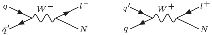
Figure 1: Feynman diagrams for the parton-level subprocesses relevant to heavy neutrino production at the LHC.

By far the cleanest signals come from the heavy neutrinos decaying as $N\to l^{\pm}W^{\mp}\to l^{\pm}jj$, with $l=e,\mu$ and $j$ representing a hadronic jet. All the decay products can then be detected, allowing the reconstruction of the invariant mass, and more importantly, the observation of lepton-flavour and lepton-number violation. Given this decay chain, signals that conserve $L$ will be of the form $pp\to l^{\pm}l^{\prime\mp}W^{\pm}X$, where here $X$ represents the beam remnants and the $W$ boson is assumed to decay hadronically. In addition to these, for Majorana neutrinos only, LNV processes of the form $pp\to l^{\pm}l^{\prime\pm}W^{\mp}X$ are also possible. If observed, this would unravel the Dirac or Majorana nature of the heavy neutrinos.

In order to suppress the SM background, signals for heavy neutrinos must be LFV (which includes any LNV processes). Since both lepton-flavour and lepton-number violation are forbidden in the SM, the backgrounds to these processes require extra light neutrinos in the final state. The main source of this type of background will come from three $W$ bosons. If two of these decay leptonically and the third hadronically, this can mimic the signal apart from the additional light neutrinos. Recent analyses of this process have concluded that such a background can be made negligible after cuts [11, 12]. In particular, a missing $p_{T}$ cut is very effective, since this should have no effect on the signal.

4 The Resummed Heavy Neutrino Propagator

CP violation may originate from self-energy, vertex or higher order quantum corrections. In general these are small effects, since electroweak loop corrections themselves are small. However, if two or more of the heavy neutrinos are nearly degenerate in mass, then CP violation from self-energy corrections (often termed $\epsilon$-type CP violation [19]) can be resonantly enhanced [22]. In fact, in the limit of degenerate heavy neutrinos, finite-order perturbation theory breaks down. A well defined field-theoretic formalism is based on a resummation of the self-energy graphs [29, 22]. This approach is manifestly gauge invariant within the Pinch Technique (PT) framework [61, 65] and maintains other field-theoretic properties, such as unitarity and CPT invariance. Our formalism involves the absorptive part of the heavy neutrino self-energy, which is computed here at the one-loop level. An important point regarding this formalism is that both the diagonal and off-diagonal elements of the self-energy must be inserted into the heavy neutrino propagator matrix. This is crucial, since for small mass-splittings, the off-diagonal elements play a major role.

Following this approach, the propagator for a system of two heavy neutrinos is given by

$$\hat{S}(\not{p})=\left[\begin{array}[]{cc}\not{p}-m_{1}+i{\rm Im}\,\hat{\Sigma}_{11}(\not{p})&i{\rm Im}\,\hat{\Sigma}_{12}(\not{p})\\ i{\rm Im}\,\hat{\Sigma}_{21}(\not{p})&\not{p}-m_{2}+i{\rm Im}\,\hat{\Sigma}_{22}(\not{p})\end{array}\right]^{-1},$$ (4.1)

where ${\rm Im}\,\hat{\Sigma}_{ij}(\not{p})$ is the absorptive part of the heavy neutrino self-energy.

4.1 Majorana neutrinos

For Majorana neutrinos, ${\rm Im}\,\hat{\Sigma}_{ij}(\not{p})$ is of the form

$${\rm Im}\,\hat{\Sigma}_{ij}(\not{p})=A_{ij}(s)\not{p}P_{L}+A^{*}_{ij}(s)\not{p}P_{R}\,,$$ (4.2)

where $s=p^{2}$ and $A(s)$ is Hermitian, (i.e. $A_{ij}=A^{*}_{ji}$).

Writing the propagator as

$$\hat{S}_{M}(\not{p})=D_{M}(s)\not{p}P_{L}+E_{M}(s)\not{p}P_{R}+F_{M}(s)P_{L}+G_{M}(s)P_{R}\,,$$ (4.3)

the matrices $D_{M}$, $E_{M}$, $F_{M}$ and $G_{M}$ are given by

$$D_{M} = \frac{1}{Z_{M}}\left(\begin{array}[]{cc}X_{22}\tilde{A}_{11}+s|A_{12}|^{2}\tilde{A}_{22}&-i(sA_{21}Y+m_{1}m_{2}A_{12})\\ -i(sA_{12}Y+m_{1}m_{2}A_{21})&X_{11}\tilde{A}_{22}+s|A_{12}|^{2}\tilde{A}_{11}\end{array}\right),$$ (4.6)

$$E_{M} = \frac{1}{Z_{M}}\left(\begin{array}[]{cc}X_{22}\tilde{A}_{11}+s|A_{12}|^{2}\tilde{A}_{22}&-i(sA_{12}Y+m_{1}m_{2}A_{21})\\ -i(sA_{21}Y+m_{1}m_{2}A_{12})&X_{11}\tilde{A}_{22}+s|A_{12}|^{2}\tilde{A}_{11}\end{array}\right),$$ (4.9)

$$F_{M} = \frac{1}{Z_{M}}\left(\begin{array}[]{cc}X_{22}m_{1}-sm_{2}A^{2}_{12}&-is(m_{1}A_{21}\tilde{A}_{22}+m_{2}A_{12}\tilde{A}_{11})\\ -is(m_{1}A_{21}\tilde{A}_{22}+m_{2}A_{12}\tilde{A}_{11})&X_{11}m_{2}-sm_{1}A^{2}_{21}\end{array}\right),\hskip 28.45274pt$$ (4.12)

$$G_{M} = \frac{1}{Z_{M}}\left(\begin{array}[]{cc}X_{22}m_{1}-sm_{2}A^{2}_{21}&-is(m_{1}A_{12}\tilde{A}_{22}+m_{2}A_{21}\tilde{A}_{11})\\ -is(m_{1}A_{12}\tilde{A}_{22}+m_{2}A_{21}\tilde{A}_{11})&X_{11}m_{2}-sm_{1}A^{2}_{12}\end{array}\right),$$ (4.15)

where

$$\tilde{A}_{ii}=1+iA_{ii}\,;\hskip 28.45274ptX_{ii}=s\tilde{A}^{2}_{ii}-m^{2}_{i}\,;\hskip 28.45274ptY=|A_{12}|^{2}+\tilde{A}_{11}\tilde{A}_{22}\,;$$

$$Z_{M}=X_{11}X_{22}+sm_{1}m_{2}(A^{2}_{12}+A^{2}_{21})+s^{2}|A_{12}|^{2}(2\tilde{A}_{11}\tilde{A}_{22}+|A_{12}|^{2})\,.$$ (4.16)

By inspection, it can be seen that $E_{M}$ is related to $D_{M}$, and $G_{M}$ to $F_{M}$ through

$$E_{M}[A^{*}]=D_{M}[A]\,;\hskip 22.76228ptG_{M}[A^{*}]=F_{M}[A]\,;\hskip 22.76228ptE_{M}=D_{M}^{T}\,;\hskip 22.76228ptF_{M}=F_{M}^{T}\,;\hskip 22.76228ptG_{M}=G_{M}^{T}\,.$$ (4.17)

Defining the matrices $M$ and $\tilde{A}$ as

$$M=\left(\begin{array}[]{cc}m_{1}&0\\ 0&m_{2}\end{array}\right);\hskip 28.45274pt\tilde{A}=\left(\begin{array}[]{cc}1+iA_{11}&iA_{12}\\ iA_{21}&1+iA_{22}\end{array}\right),$$ (4.18)

Eq. (4.1) can be written

$$\hat{S}_{M}^{-1}(\not{p})=\tilde{A}\not{p}P_{L}+\tilde{A}^{T}\not{p}P_{R}-M\,.$$ (4.19)

Combining this with (4.3), the property $SS^{-1}=1$ gives the further equalities

$$sE_{M}\tilde{A}-F_{M}M=1\,;\hskip 22.76228ptsD_{M}\tilde{A}^{T}-G_{M}M=1\,;\hskip 22.76228ptG_{M}\tilde{A}=D_{M}M\,;\hskip 22.76228ptF_{M}\tilde{A}^{T}=E_{M}M\,.$$ (4.20)

These relations, which can be directly verified for the matrices given in (4.6)–(4.15) are important for checking that CPT invariance is preserved in the theory. More details will be given in Section 5.

4.2 Dirac neutrinos

For Dirac neutrinos, the absorptive part of their self-energy has only the left-handed component, viz

$${\rm Im}\,\hat{\Sigma}_{ij}(\not{p})=A_{ij}(s)\not{p}P_{L}\,.$$ (4.21)

Writing the propagator in the same form as that in (4.3), i.e.

$$\hat{S}_{D}(\not{p})=D_{D}(s)\not{p}P_{L}+E_{D}(s)\not{p}P_{R}+F_{D}(s)P_{L}+G_{D}(s)P_{R}\,,$$ (4.22)

the matrices $D_{D}$, $E_{D}$, $F_{D}$ and $G_{D}$ are given by the expressions

$$D_{D} = \frac{1}{Z_{D}}\left(\begin{array}[]{cc}(s\tilde{A}_{22}-m_{2}^{2})\tilde{A}_{11}+s|A_{12}|^{2}&-iA_{12}m_{1}m_{2}\\ -iA_{21}m_{1}m_{2}&(s\tilde{A}_{11}-m_{1}^{2})\tilde{A}_{22}+s|A_{12}|^{2}\end{array}\right),$$ (4.25)

$$E_{D} = \frac{1}{Z_{D}}\left(\begin{array}[]{cc}s\tilde{A}_{22}-m_{2}^{2}&-isA_{12}\\ -isA_{21}&s\tilde{A}_{11}-m_{1}^{2}\end{array}\right),$$ (4.28)

$$F_{D} = \frac{1}{Z_{D}}\left(\begin{array}[]{cc}(s\tilde{A}_{22}-m_{2}^{2})m_{1}&-ism_{2}A_{12}\\ -ism_{1}A_{21}&(s\tilde{A}_{11}-m_{1}^{2})m_{2}\end{array}\right),$$ (4.31)

$$G_{D} = \frac{1}{Z_{D}}\left(\begin{array}[]{cc}(s\tilde{A}_{22}-m_{2}^{2})m_{1}&-ism_{1}A_{12}\\ -ism_{2}A_{21}&(s\tilde{A}_{11}-m_{1}^{2})m_{2}\end{array}\right),$$ (4.34)

with

$$Z_{D}=(s\tilde{A}_{11}-m_{1}^{2})(s\tilde{A}_{22}-m_{2}^{2})+s^{2}|A_{12}|^{2}\,,$$ (4.35)

and $\tilde{A}_{ii}$ defined in (4.16).

The inverse propagator can be expressed as

$$\hat{S}_{D}^{-1}(\not{p})=\tilde{A}\not{p}P_{L}+\not{p}P_{R}-M\,,$$ (4.36)

so the equivalent of the relations in (4.20) for Dirac neutrinos are

$$sE_{D}\tilde{A}-F_{D}M=1\,;\hskip 28.45274ptsD_{D}-G_{D}M=1\,;\hskip 28.45274ptG_{D}\tilde{A}=D_{D}M\,;\hskip 28.45274ptF_{D}=E_{D}M\,.$$ (4.37)

Calculating the absorptive part of the self-energy at one-loop level in the Feynman-’t Hooft gauge (for which the Feynman graphs are given in Fig. 2), the matrix $A(s)$, which is the same for both Dirac and Majorana neutrinos, is given by

$$A_{ij}(s)\! = \!\frac{g^{2}}{128\pi s^{2}M_{W}^{2}}\Bigg{\{}\,C_{ij}\,\Bigg{[}\,4M_{W}^{2}(s-M_{W}^{2})^{2}\theta(s-M_{W}^{2})\>+\>2M_{Z}^{2}(s-M_{Z}^{2})^{2}\theta(s-M_{Z}^{2})\Bigg{]}$$

$$+\>m_{i}m_{j}\,C^{*}_{ij}\,\Bigg{[}\,2(s-M_{W}^{2})^{2}\theta(s-M_{W}^{2})+(s-M_{Z}^{2})^{2}\theta(s-M_{Z}^{2})\>+\>(s-M_{H}^{2})^{2}\theta(s-M_{H}^{2})\,\Bigg{]}\,\Bigg{\}}\;.$$

The tree-level heavy neutrino widths can then be obtained through $\Gamma_{N_{i}}=m_{i}A_{ii}(m_{i}^{2})$ for Dirac neutrinos and $\Gamma_{N_{i}}=2m_{i}A_{ii}(m_{i}^{2})$ for Majorana neutrinos.

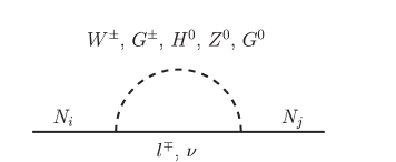
Figure 2: Feynman graphs contributing to the one-loop self-energy of heavy neutrinos. For Dirac neutrinos, only the LNC graphs exist.

5 CP Asymmetries in $lW\to l^{\prime}W$ Type Processes

For the LHC signals described in Section 3, the heavy neutrino propagator is coupled to a charged lepton and $W$ boson at each end. The asymmetries between such processes and their CP-conjugates will thus be the same as for the $2\to 2$ processes $lW\to l^{\prime}W$. This can be understood since the fermion line containing the heavy neutrino is the same in the Feynman graphs for both the $2\to 3$ signals and the corresponding $2\to 2$ processes. The fact that one of the charged leptons changes from being a final state particle to an initial state particle will not effect much the size of the CP asymmetries.

As a result of CPT invariance, if all possible final states $X$ are summed over, then [29]

$$\sigma(l^{+}W^{-}\to N\to X)=\sigma(l^{-}W^{+}\to N\to X).$$ (5.1)

However, it is possible for the asymmetry between the cross sections for producing any particular final state and its CP-conjugate to be large.

Considering LNC processes first, the CP-violating difference between $\sigma(q\bar{q}^{\prime}\to l^{+}l^{\prime-}W^{+})$ and $\sigma(\bar{q}q^{\prime}\to l^{-}l^{\prime+}W^{-})$ will thus be proportional to that between $\sigma(l^{-}W^{+}\to l^{\prime-}W^{+})$ and $\sigma(l^{+}W^{-}\to l^{\prime+}W^{-})$. The only relevant parts of the cross sections are those that involve the couplings of the heavy neutrinos, any pair of CP-conjugate processes will be otherwise identical. Therefore, this asymmetry will be proportional to the factors

$$\Delta_{\rm CP}^{\rm LNC}|_{\rm Dirac} = \left|B_{l^{\prime}}E_{D}(s)B_{l}^{\dagger}\right|^{2}-\left|B_{l}E_{D}(s)B_{l^{\prime}}^{\dagger}\right|^{2}\,,$$ (5.2)

$$\Delta_{\rm CP}^{\rm LNC}|_{\rm Majorana} = \left|B_{l^{\prime}}E_{M}(s)B_{l}^{\dagger}\right|^{2}-\left|B_{l}E_{M}(s)B_{l^{\prime}}^{\dagger}\right|^{2}\,,$$ (5.3)

depending on whether the heavy neutrino is a Dirac or Majorana particle. In the above, $B_{l}=(B_{l1},B_{l2})$ with $N_{1}$ and $N_{2}$ being the two nearly degenerate heavy neutrinos involved. As is a direct consequence of CPT invariance, these vanish if $l$ and $l^{\prime}$, the two charged leptons that the heavy neutrinos couple to, are the same. Since $E[B^{*}]=E^{T}[B]$ for both Dirac and Majorana neutrinos, the two terms in $\Delta_{\rm CP}^{\rm LNC}$ transform into each other under $B\to B^{*}$, hence confirming that they represent CP-conjugates. Using the expression for $E_{D}$ given in (4.28), $\Delta_{\rm CP}^{\rm LNC}|_{\rm Dirac}$ is given by

$$\Delta_{\rm CP}^{\rm LNC}|_{\rm Dirac} = \frac{4s(s-m_{2}^{2})}{|Z_{D}|^{2}}\left(A_{11}{\rm Im}[B^{*}_{l1}B_{l^{\prime}1}B_{l2}B^{*}_{l^{\prime}2}]\right.$$ (5.4)

$$\left.-|B_{l1}|^{2}{\rm Im}[A_{12}B_{l^{\prime}1}B^{*}_{l^{\prime}2}]+|B_{l^{\prime}1}|^{2}{\rm Im}[A_{12}B_{l1}B^{*}_{l2}]\right)$$

$$+\,(1\leftrightarrow 2)\,.$$

The full expression for $\Delta_{\rm CP}^{\rm LNC}|_{\rm Majorana}$ is rather more complicated, it is thus pragmatic to work with an approximation when performing analytic calculations. The elements of $A$ are very small (of order the heavy neutrino widths divided by their masses), so terms above first order in them can be dropped to a very good approximation. Doing this, the matrix $E_{M}$ is approximated as

$$E_{M}\approx\frac{1}{Z_{M}}\left(\begin{array}[]{cc}(s-m_{2}^{2})\tilde{A}_{11}+2isA_{22}&-i(sA_{12}+m_{1}m_{2}A_{21})\\ -i(sA_{21}+m_{1}m_{2}A_{12})&(s-m_{1}^{2})\tilde{A}_{22}+2isA_{11}\end{array}\right).$$ (5.5)

Using this approximation, $\Delta_{\rm CP}^{\rm LNC}|_{\rm Majorana}$ is given by

$$\Delta_{\rm CP}^{\rm LNC}|_{\rm Majorana} = \frac{4(s-m_{2}^{2})}{|Z_{M}|^{2}}\left[(s+m_{1}^{2})A_{11}{\rm Im}[B^{*}_{l1}B_{l^{\prime}1}B_{l2}B^{*}_{l^{\prime}2}]\right.$$ (5.6)

$$-|B_{l1}|^{2}(s{\rm Im}[A_{12}B_{l^{\prime}1}B^{*}_{l^{\prime}2}]+m_{1}m_{2}{\rm Im}[A_{21}B_{l^{\prime}1}B^{*}_{l^{\prime}2}])$$

$$\left.+|B_{l^{\prime}1}|^{2}(s{\rm Im}[A_{12}B_{l1}B^{*}_{l2}]+m_{1}m_{2}{\rm Im}[A_{21}B_{l1}B^{*}_{l2}])\right]$$

$$+\,(1\leftrightarrow 2)\,.$$

The propagator for Dirac neutrinos simply contains a subset of the terms in the corresponding one for Majorana neutrinos, the same is thus also true of the CP-violating expressions (5.4) and (5.6). The extra terms that appear for Majorana neutrinos all have an $m^{2}$ mass dependence, these are due to interference between graphs without a chirality flip in them and graphs with a double chirality flip, the latter not appearing for Dirac neutrinos. There will also be higher order (in the elements of $A$) terms for Majorana neutrinos that have been neglected in our approximation for $E_{M}$.

An analogous expression can be derived for the LNV signals (assuming neutrinos are Majorana particles so such processes are allowed), which are of the form $\sigma(q\bar{q}^{\prime}\to l^{\pm}l^{\prime\pm}W^{\mp})$. The asymmetries between these signals are related to those between $\sigma(l^{-}W^{+}\to l^{\prime+}W^{-})$ and $\sigma(l^{+}W^{-}\to l^{\prime-}W^{+})$, which are proportional to

$$\Delta_{\rm CP}^{\rm LNV}=\left|B^{*}_{l^{\prime}}G_{M}(s)B_{l}^{\dagger}\right|^{2}-\left|B_{l}F_{M}(s)B_{l^{\prime}}^{T}\right|^{2}\,,$$ (5.7)

where only the contributions from the resonant $s$-channel diagrams are included. $F_{M}(s)$ and $G_{M}(s)$ are symmetric, so both terms in this expression are individually invariant under $l\leftrightarrow l^{\prime}$. Also, since $G_{M}[B^{*}]=F_{M}[B]$, it can again be confirmed that these terms represent CP-conjugates, since they transform into each other under $B\to B^{*}$.

In order to make the expressions manageable, we will continue to work with an approximation of the heavy Majorana neutrino propagator that drops higher order terms in the elements of the matrix $A$. With this approximation, the matrices $F_{M}$ and $G_{M}$ are given by

$$F_{M} \approx \frac{1}{Z_{M}}\left(\begin{array}[]{cc}m_{1}(s(1+2iA_{22})-m^{2}_{2})&-is(m_{1}A_{21}+m_{2}A_{12})\\ -is(m_{1}A_{21}+m_{2}A_{12})&m_{2}(s(1+2iA_{11})-m^{2}_{1})\end{array}\right),$$ (5.10)

$$G_{M} \approx \frac{1}{Z_{M}}\left(\begin{array}[]{cc}m_{1}(s(1+2iA_{22})-m^{2}_{2})&-is(m_{1}A_{12}+m_{2}A_{21})\\ -is(m_{1}A_{12}+m_{2}A_{21})&m_{2}(s(1+2iA_{11})-m^{2}_{1})\end{array}\right).$$ (5.13)

Using these expressions, the CP asymmetry for LNV processes of the type considered is

$$\Delta_{\rm CP}^{\rm LNV} = \frac{4sm_{1}(s-m_{2}^{2})}{|Z_{M}|^{2}}\bigg{[}2m_{2}A_{11}{\rm Im}[B_{l1}^{*}B_{l^{\prime}1}^{*}B_{l2}B_{l^{\prime}2}]$$ (5.14)

$$+|B_{l1}|^{2}\left(m_{1}{\rm Im}[A_{12}B_{l^{\prime}1}B^{*}_{l^{\prime}2}]+m_{2}{\rm Im}[A_{21}B_{l^{\prime}1}B^{*}_{l^{\prime}2}]\right)$$

$$+|B_{l^{\prime}1}|^{2}\left(m_{1}{\rm Im}[A_{12}B_{l1}B^{*}_{l2}]+m_{2}{\rm Im}[A_{21}B_{l1}B^{*}_{l2}]\right)\bigg{]}$$

$$+\,(1\leftrightarrow 2)\,.$$

Since all first order graphs contributing to LNV processes have a single chirality flip in the propagator, all the terms in the above expression are proportional to $m^{2}$.

5.1 Theoretical constraints (for Majorana neutrinos)

For three heavy Majorana neutrinos, $B_{lN}$ is a $3\times 3$ matrix. Ignoring the light neutrino masses, the constraints in (2.24) thus leave four of the heavy neutrino couplings as free parameters. For example, $B_{l1}$ ($l=e,\mu,\tau$) and $B_{e2}$ can be chosen, Eq. (2.24) is then satisfied by

$$B_{e3}=\pm i\sqrt{\frac{m_{1}B_{e1}^{2}+m_{2}B_{e2}^{2}}{m_{3}}}\,;\hskip 28.45274ptB_{li}=\frac{B_{l1}B_{ei}}{B_{e1}}\,.$$ (5.15)

In order to see how this effects the expressions for the $\Delta_{\rm CP}$’s, we write the absorptive self-energy matrix $A$ given in (4.2) as follows:

$$A_{ij}\ =\ C_{ij}\,a(s)\>+\>C^{*}_{ij}\,\frac{m_{i}m_{j}}{M_{W}^{2}}\;b(s)\;,$$ (5.16)

where $a$ and $b$ are dimensionless real functions. Then, using (2.23)

$${\rm Im}[A_{ij}B_{l1}B^{*}_{l2}]\ =\ \sum_{l^{\prime}}\>\Bigg{(}a\,{\rm Im}[B_{l^{\prime}i}^{*}B_{l^{\prime}j}B_{l1}B^{*}_{l2}]\>+\>b\,\frac{m_{i}m_{j}}{M_{W}^{2}}\,{\rm Im}[B_{l^{\prime}i}B^{*}_{l^{\prime}j}B_{l1}B^{*}_{l2}]\,\Bigg{)}\;,$$ (5.17)

which, after the application of (5.15), becomes

$${\rm Im}[A_{ij}B_{l1}B^{*}_{l2}]\ =\ C_{11}\frac{|B_{l1}|^{2}}{|B_{e1}|^{4}}\left(a\,{\rm Im}\left[B_{ei}^{*}B_{ej}B_{e1}B^{*}_{e2}\right]\>+\>b\frac{m_{i}m_{j}}{M_{W}^{2}}\;{\rm Im}\left[B_{ei}B^{*}_{ej}B_{e1}B^{*}_{e2}\right]\,\right)\;.$$ (5.18)

Inserting this into (5.6), $\Delta_{\rm CP}^{\rm LNC}|_{\rm Majorana}$ can be shown to vanish, while in (5.14), all terms proportional to $a$ cancel out and we are left with

$$\Delta_{\rm CP}^{\rm LNV}=\frac{8bsm_{1}m_{2}(m_{1}-m_{2})|B_{l1}|^{2}|B_{l^{\prime}1}|^{2}C_{11}}{M_{W}^{2}|Z_{M}|^{2}}\left(\frac{|B_{e2}|^{2}}{|B_{e1}|^{2}}m_{2}(s-m_{1}^{2})+m_{1}(s-m_{2}^{2})\right){\rm Im}\left[\left(\frac{B_{e2}}{B_{e1}}\right)^{2}\right],$$ (5.19)

where

$$b=\frac{g^{2}(2(s-M_{W}^{2})^{2}\theta(s-M_{Z}^{2})+(s-M_{Z}^{2})^{2}\theta(s-M_{Z}^{2})+(s-M_{H}^{2})^{2}\theta(s-M_{H}^{2}))}{128\pi s^{2}}\,.$$ (5.20)

For neutrino masses accessible to colliders this is always very small, so no observable CP violation is possible for the model considered with three heavy Majorana neutrinos. This result holds as long as only two of them are close enough in mass to have significant mixing in the propagator. The case of all three neutrinos being nearly degenerate is more involved, so whether large CP asymmetries can occur in this case may be studied elsewhere.

If at least four heavy neutrinos exist, Eq. (2.24) can be satisfied for any choices of the couplings of the two quasi-degenerate neutrinos. Scenarios which result in large CP asymmetries are thus possible, and it is in the context of such a theory which our numerical results for Majorana neutrinos are to be considered. As mentioned in Section 2.2, Eq. (2.24) is automatically satisfied for the model with Dirac neutrinos. As such, even with just two heavy neutrinos, large CP asymmetries can result here.

5.2 Scenarios with large CP asymmetries

For the purposes of our numerical calculations, we assume the couplings of the nearly degenerate neutrinos can be chosen independently for both Dirac and Majorana neutrinos. Although this implies at least four heavy neutrinos in the Majorana case, we also assume that only two of these are close in mass, such that we can use our $2\times 2$ propagators given in Section 4. In order to determine scenarios which would result in large CP asymmetries, we consider just the kinematic point $s=\overline{s}=\frac{1}{2}(m_{1}^{2}+m_{2}^{2})$. To further simplify the expressions, we will also set the heavy neutrino couplings to all have a common magnitude $|B|$.

Introducing the notation $\Delta_{\rm CP}(\overline{s})\equiv\overline{\Delta}_{\rm CP}$, $Z(\overline{s})\equiv\overline{Z}$ and $A_{ij}(\overline{s})\equiv\overline{A}_{ij}$, the CP asymmetry for Dirac neutrinos is given by

$$\overline{\Delta}_{\rm CP}^{\rm LNC}|_{\rm Dirac} = \frac{m_{1}^{4}-m_{2}^{4}}{|\overline{Z}_{D}|^{2}}\left[(\overline{A}_{11}+\overline{A}_{22}){\rm Im}[B^{*}_{l1}B_{l^{\prime}1}B_{l2}B^{*}_{l^{\prime}2}]-\right.$$ (5.21)

$$\left.(|B_{l1}|^{2}+|B_{l2}|^{2}){\rm Im}[\overline{A}_{12}B_{l^{\prime}1}B^{*}_{l^{\prime}2}]+(|B_{l^{\prime}1}|^{2}+|B_{l^{\prime}2}|^{2}){\rm Im}[\overline{A}_{12}B_{l1}B^{*}_{l2}]\right].$$

One way to obtain a large value for this expression is to maximise ${\rm Im}[B^{*}_{l1}B_{l^{\prime}1}B_{l2}B^{*}_{l^{\prime}2}]$, which can be done by having one of the four couplings imaginary and the rest real. The couplings to the third charged lepton (i.e. not $l$ or $l^{\prime}$) can then be chosen such that $C_{12}$ is either real or imaginary, and so either ${\rm Im}[\overline{A}_{12}B_{l^{\prime}1}B^{*}_{l^{\prime}2}]$ or ${\rm Im}[\overline{A}_{12}B_{l1}B^{*}_{l2}]$ will be zero. If we now impose the condition that all the couplings have the same magnitude $|B|$, Eq. (5.21) becomes

$$\left|\overline{\Delta}_{\rm CP}^{\rm LNC}|_{\rm Dirac}\right| = \frac{|B|^{4}}{|\overline{Z}_{D}|^{2}}(\overline{A}_{11}+\overline{A}_{22}-2|\overline{A}_{12}|)|m_{1}^{4}-m_{2}^{4}|\,.$$ (5.22)

Although there is a partial cancellation between the elements of $\overline{A}$, the off-diagonal element will only be about one third of the magnitude of the diagonal elements (which are approximately equal). This is because in $\overline{A}_{12}$, the contribution from the couplings to the third charged lepton cancel exactly with the contribution from either $l$ or $l^{\prime}$. The equality $\overline{A}_{11}=\overline{A}_{22}=3|\overline{A}_{12}|$ is not exact however, since there are small differences due to the mass-splitting of the two heavy neutrinos.

For Majorana neutrinos, the expression for $\overline{\Delta}_{\rm CP}^{\rm LNC}|_{\rm Majorana}$ is

$$\overline{\Delta}_{\rm CP}^{\rm LNC}|_{\rm Majorana} = \frac{m_{1}^{2}-m_{2}^{2}}{|\overline{Z}_{M}|^{2}}\left[\left((3m_{1}^{2}+m_{2}^{2})\overline{A}_{11}+(m_{1}^{2}+3m_{2}^{2})\overline{A}_{22}\right){\rm Im}[B^{*}_{l1}B_{l^{\prime}1}B_{l2}B^{*}_{l^{\prime}2}]\right.$$ (5.23)

$$-(|B_{l1}|^{2}+|B_{l2}|^{2})\left((m_{1}^{2}+m_{2}^{2}){\rm Im}[\overline{A}_{12}B_{l^{\prime}1}B^{*}_{l^{\prime}2}]+2m_{1}m_{2}{\rm Im}[\overline{A}_{21}B_{l^{\prime}1}B^{*}_{l^{\prime}2}]\right)$$

$$\left.+(|B_{l^{\prime}1}|^{2}+|B_{l^{\prime}2}|^{2})\left((m_{1}^{2}+m_{2}^{2}){\rm Im}[\overline{A}_{12}B_{l1}B^{*}_{l2}]+2m_{1}m_{2}{\rm Im}[\overline{A}_{21}B_{l1}B^{*}_{l2}]\right)\right].\hskip 5.69046pt$$

If $\overline{A}_{12}$ is imaginary, then ${\rm Im}[\overline{A}_{12}B_{l1}B^{*}_{l2}]=-{\rm Im}[\overline{A}_{21}B_{l1}B^{*}_{l2}]$. Under the same assumption for the $B$-couplings, we find

$$\left|\overline{\Delta}_{\rm CP}^{\rm LNC}|_{\rm Majorana}\right| = \frac{|m_{1}^{2}-m_{2}^{2}||B|^{4}}{|\overline{Z}_{M}|^{2}}\left((3m_{1}^{2}+m_{2}^{2})\overline{A}_{11}+(m_{1}^{2}+3m_{2}^{2})\overline{A}_{22}\right)+\mathcal{O}\left[(m_{1}-m_{2})^{2}\right].\hskip 5.69046pt$$ (5.24)

For LNV processes, $\overline{\Delta}_{\rm CP}^{\rm LNV}$ is given by

$$\overline{\Delta}_{\rm CP}^{\rm LNV} = \frac{m_{1}^{4}-m_{2}^{4}}{|\overline{Z}_{M}|^{2}}\bigg{[}2m_{1}m_{2}(\overline{A}_{11}+\overline{A}_{22}){\rm Im}[B_{l1}^{*}B_{l^{\prime}1}^{*}B_{l2}B_{l^{\prime}2}]$$ (5.25)

$$+\left((m_{1}^{2}|B_{l1}|^{2}+m_{2}^{2}|B_{l2}|^{2}){\rm Im}[\overline{A}_{12}B_{l^{\prime}1}B^{*}_{l^{\prime}2}]+m_{1}m_{2}(|B_{l1}|^{2}+|B_{l2}|^{2}){\rm Im}[\overline{A}_{21}B_{l^{\prime}1}B^{*}_{l^{\prime}2}]\right)$$

$$+\left((m_{1}^{2}|B_{l^{\prime}1}|^{2}+m_{2}^{2}|B_{l^{\prime}2}|^{2}){\rm Im}[\overline{A}_{12}B_{l1}B^{*}_{l2}]+m_{1}m_{2}(|B_{l^{\prime}1}|^{2}+|B_{l^{\prime}2}|^{2}){\rm Im}[\overline{A}_{21}B_{l1}B^{*}_{l2}]\right)\bigg{]}.\hskip 17.07182pt$$

As long as $l\neq l^{\prime}$, then the same assumptions for the couplings lead to

$$\left|\overline{\Delta}_{\rm CP}^{\rm LNV}\right| = \frac{2m_{1}m_{2}|B|^{4}}{|\overline{Z}_{M}|^{2}}(\overline{A}_{11}+\overline{A}_{22})|m_{1}^{4}-m_{2}^{4}|+\mathcal{O}\left[(m_{1}-m_{2})^{2}\right].$$ (5.26)

If $l=l^{\prime}$, then

$$\overline{\Delta}_{\rm CP}^{\rm LNV} = \frac{m_{1}^{4}-m_{2}^{4}}{|\overline{Z}_{M}|^{2}}\bigg{[}2m_{1}m_{2}(\overline{A}_{11}+\overline{A}_{22}){\rm Im}[(B_{l1}^{*}B_{l2})^{2}]$$ (5.27)

$$+2\left((m_{1}^{2}|B_{l1}|^{2}+m_{2}^{2}|B_{l2}|^{2}){\rm Im}[\overline{A}_{12}B_{l1}B^{*}_{l2}]+m_{1}m_{2}(|B_{l1}|^{2}+|B_{l2}|^{2}){\rm Im}[\overline{A}_{21}B_{l1}B^{*}_{l2}]\right).\hskip 8.5359pt$$

The easiest way to get a large value for this is to have $B_{l1}B^{*}_{l2}$ imaginary. ${\rm Im}[(B_{l1}^{*}B_{l2})^{2}]$ is then zero, but both ${\rm Im}[\overline{A}_{12}B_{l1}B^{*}_{l2}]$ and ${\rm Im}[\overline{A}_{21}B_{l1}B^{*}_{l2}]$ will be large (and of the same sign), as long as $C_{12}$ has a significant real component. The asymmetry is then

$$\left|\overline{\Delta}_{\rm CP}^{\rm LNV}\right| = \frac{2|B|^{4}}{|\overline{Z}_{M}|^{2}}|m_{1}^{4}-m_{2}^{4}|(m_{1}+m_{2})^{2}{\rm Re}[\overline{A}_{12}]\,.$$ (5.28)

In all the above coupling scenarios, if the heavy neutrino mass-splitting $\Delta m_{N}\equiv m_{2}-m_{1}$ is of order their widths, then the CP asymmetries can be of order the cross sections involved. In the resonant region, these have terms proportional to either ${\Delta m}^{2}$, $\Gamma_{N}^{2}$ or $\Delta m\,\Gamma_{N}$ (all over $|\overline{Z}_{D/M}|^{2}$). The CP asymmetries are themselves proportional to $\Delta m\,\Gamma_{N}$ (over $|\overline{Z}_{D/M}|^{2}$), so for $\Delta m\approx\Gamma_{N}$, CP violation can be resonant. This still requires particular coupling scenarios such as we have described, but since we are interested in investigating the possibility of large CP asymmetries at the LHC, we will use these optimised conditions for our numerical studies.

6 Numerical Results

In this section we give our numerical results for the cross sections of the various signals of the type discussed in Section 3, for clarity, we list these in Table 1. As mentioned in Section 3, in all signals considered, the $W$ bosons are assumed to decay hadronically. We do not consider $\tau$ leptons as possible final state particles since these decay before reaching the detector and so would require a more involved analysis. Since we are primarily interested in CP asymmetries between the signal processes, we also plot these, which we define in later this section and also include in Table 1. For the results shown, we have used the CTEQ6M PDF’s [27], in which we have used $Q=m_{N}$. Setting $Q$ equal to the invariant mass of the $W^{*}$ instead, for example, increases the cross sections slightly for relatively low heavy neutrino masses.

The basic assumption required for our calculations to be valid is that the two quasi-degenerate heavy neutrinos are the only new physics particles that make an appreciable contribution to the processes considered. All others are assumed to either not couple to relevant particles, or have masses $\gtrsim 1\,{\rm TeV}$. Our calculations depend weakly on the mass of the Higgs boson, for which we have used $M_{H}=120\,{\rm GeV}$, and we have globally applied the cuts $p_{T}>15\,{\rm GeV}$ and $|\eta|>2.5$ for all final state particles. Note that these kinematical cuts are similar to those chosen in [11].

We consider the following three scenarios:

(S1):

$B_{lN}=0.05$ for $l=e,\mu,\tau$ and $N=1,2$.

(S2):

As (S1), except $B_{e2}=0.05i$.

(S3):

As (S1), except $B_{\mu 2}=0.05i$ and $B_{\tau 2}=-0.05$.

The first scenario, where all couplings are real, is the CP-conserving limit. This enables us to separate true CP asymmetries from the asymmetry due to the PDF’s. The second two are chosen specifically as examples of resonant CP violation, as guided by our analysis in Section 5.2. Scenario (S2) gives rise to large asymmetries for Majorana neutrinos, but not for Dirac neutrinos, whereas in scenario (S3) large CP asymmetries occur for both Dirac and Majorana neutrinos, but only if the two final state charged leptons are of different flavour.

Including just the two heavy neutrinos that are directly involved in the signal processes, we have $\sum_{i}|B_{lN_{i}}|^{2}=0.005$ (for all $l$). This leaves room for couplings to other heavy neutrinos without invalidating the experimental limits in (2.43). This is especially important for Majorana neutrinos, since as noted in Section 5.1, it is necessary then to have at least four heavy neutrinos to avoid theoretical constraints on their couplings. In the same context, a degree of cancellation between the different loop contributions might be necessary for the scenarios (S1)–(S3) to satisfy the bounds in (2.44), especially those derived from the non-observation of $\mu\to e\gamma$.

We start our investigation of CP violation by constructing the following CP asymmetry

$$A_{\rm CP}=\frac{\sigma(pp\to(W^{+})^{*}\to S_{i})-K\sigma(pp\to(W^{-})^{*}\to\overline{S}_{i})}{\sigma(pp\to(W^{+})^{*}\to S_{i})+K\sigma(pp\to(W^{-})^{*}\to\overline{S}_{i})}\,,$$ (6.1)

where $S_{i}$ can stand for any of the signal final states considered and $\overline{S}_{i}$ its CP-conjugate. The function $K$ takes account of the different PDF’s involved in producing $W^{+}$ and $W^{-}$ bosons, such that $A_{\rm CP}=0$ if CP is conserved. It has to be calculated theoretically and is defined as

$$K=\frac{\sigma(pp\to(W^{+})^{*}\to S_{i})}{\sigma(pp\to(W^{-})^{*}\to\overline{S}_{i})}\Bigg{|}_{\not{CP}=0}\,,$$ (6.2)

where again $S_{i}$ can be any of the possible final states considered and $\overline{S}_{i}$ its CP-conjugate. An important point is that although $A_{\rm CP}$ is in general different for different $S_{i}$, $K$ is, to a very good approximation, universal whichever signal (of the type considered) is used to define it. Therefore, we calculate the cross sections in the CP-conserving limit with all couplings real, like for example in scenario (S1). $K$ is independent of the magnitudes of the couplings and mass-splitting (for $\Delta m_{N}\ll m_{N}$), so any other CP-conserving scenario would give the same value. It is plotted as a function of $m_{N_{1}}$ (the mass of the lighter of the two heavy neutrinos) in Fig. 3 along with the signal cross sections in (S1). The value of $K$ can be obtained by taking the ratio of either of the two pairs of CP-conjugate signals shown. In fact, in this special scenario, where all heavy neutrino couplings are equal, all additional signals of the type considered have the same cross section as one of the four shown. However, there is an element of theoretical uncertainty predominantly coming from the different choices of PDF’s used. For instance, using the MRST2004 PDF’s [28] instead, we find values for $K$ that differ by less than $1\%$. They are also insensitive to the factorisation scale $Q$ that is used.

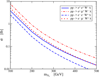
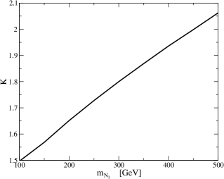
Figure 3: Left plot: Signal cross sections for scenario (S1). Right plot: The function $K$ as defined in (6.2). All additional signals of the type considered have the same cross section as one of the four shown

Another set of CP-violating observables can be constructed by considering ratios of different processes, such that the asymmetries due to the different PDF’s cancel out. Defining the ratios $R_{+}$ and $R_{-}$ as

$$R_{+}=\frac{\sigma(pp\to(W^{+})^{*}\to S_{i})}{\sigma(pp\to(W^{+})^{*}\to S_{j})}\,;\hskip 28.45274ptR_{-}=\frac{\sigma(pp\to(W^{-})^{*}\to\overline{S}_{i})}{\sigma(pp\to(W^{-})^{*}\to\overline{S}_{j})}\,,$$ (6.3)

CP-violating observables can be constructed from

$$R_{\rm CP}=\frac{R_{+}-R_{-}}{R_{+}+R_{-}}\,.$$ (6.4)

This second method has the advantage that it does not depend on $K$. However, it is more complicated to construct and analyse since two different processes (plus their CP-conjugates) are required for each asymmetry.

6.1 LNC processes

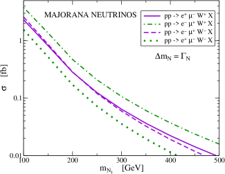
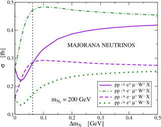
Figure 4: Cross sections for LNC signals in scenario (S2). In this scenario, no CP violation is present for Dirac neutrinos, so plots are not shown for these. In this and all other plots, the vertical dotted line represents the value of the heavy neutrino widths.

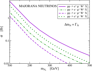
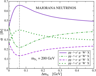
Figure 5: Cross sections for LNC signals in scenario (S3) with Majorana neutrinos.

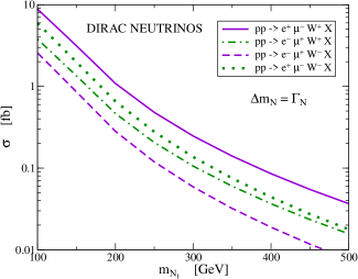
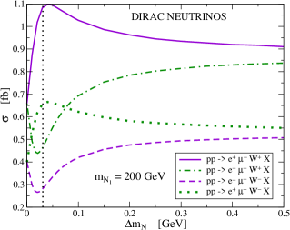
Figure 6: As Fig. 5, but with Dirac neutrinos.

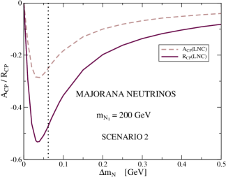
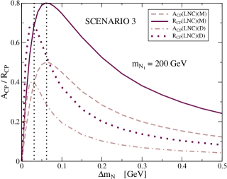
Figure 7: The CP-violating observables $A_{\rm CP}({\rm LNC})$ and $R_{\rm CP}({\rm LNC})$ as defined in (6.7) and (6.8).

We consider four distinct LNC signals, these are:

$$(1)\,pp\to e^{+}\mu^{-}W^{+}X;\hskip 14.22636pt(2)\,pp\to e^{-}\mu^{+}W^{-}X;\hskip 14.22636pt(3)\,pp\to e^{+}\mu^{-}W^{-}X;\hskip 14.22636pt(4)\,pp\to e^{-}\mu^{+}W^{+}X.$$ (6.5)

Signals (1) and (2) are CP-conjugates of each other and likewise (3) and (4). Furthermore, the cross sections for (3) and (4) are related to those for (1) and (2) through

$$\sigma(pp\to e^{\pm}\mu^{\mp}W^{+}X)=K\sigma(pp\to e^{\pm}\mu^{\mp}W^{-}X)\,,$$ (6.6)

which holds even when CP is not conserved. Using this relation, $A_{\rm CP}$ as defined in (6.1) can be expressed without involving $K$, viz

$$A_{\rm CP}({\rm LNC})=\frac{\sigma(pp\to e^{+}\mu^{-}W^{\pm}X)-\sigma(pp\to e^{-}\mu^{+}W^{\pm}X)}{\sigma(pp\to e^{+}\mu^{-}W^{\pm}X)+\sigma(pp\to e^{-}\mu^{+}W^{\pm}X)}\,.$$ (6.7)

This has also the advantage that it is not necessary to distinguish between the two $W$ boson charges experimentally. $R_{\rm CP}$, given in (6.4), can also be re-expressed using (6.6), and can thus be written as

$$R_{\rm CP}({\rm LNC})=\frac{\displaystyle{\frac{\sigma(pp\to e^{+}\mu^{-}W^{\pm}X)}{\sigma(pp\to e^{-}\mu^{+}W^{\pm}X)}-\frac{\sigma(pp\to e^{-}\mu^{+}W^{\pm}X)}{\sigma(pp\to e^{+}\mu^{-}W^{\pm}X)}}}{\displaystyle{\frac{\sigma(pp\to e^{+}\mu^{-}W^{\pm}X)}{\sigma(pp\to e^{-}\mu^{+}W^{\pm}X)}+\frac{\sigma(pp\to e^{-}\mu^{+}W^{\pm}X)}{\sigma(pp\to e^{+}\mu^{-}W^{\pm}X)}}}\,,$$ (6.8)

where again, the two charges of $W$ boson are summed over. However, the observable $R_{\rm CP}({\rm LNC})$ turns out to be closely related to $A_{\rm CP}({\rm LNC})$.

The cross sections for the signal processes given in (6.5) are shown in Fig. 4 for scenario (S2) and Figs. 5 and 6 for scenario (S3). Since scenario (S2) only results in CP violation for Majorana neutrinos, the results for Dirac neutrinos are not shown. We’ve plotted the signals as functions of $m_{N_{1}}$ and $\Delta m_{N}$. In the latter plots, the point $\Delta m_{N}=\Gamma_{N}$ is marked by a vertical dotted line. The CP asymmetries are close to their maxima at this point, which we use for our plots against $m_{N_{1}}$. The CP-violating observables given in (6.7) and (6.8) are shown as functions of $\Delta m_{N}$ in Fig. 7. Again the point $\Delta m_{N}=\Gamma_{N}$ is marked by vertical dotted lines (one each for Dirac and Majorana neutrinos).

6.2 LNV processes

We now analyse the LNV processes:

$$(1)\,pp\to e^{+}e^{+}W^{-}X;\hskip 14.22636pt(2)\,pp\to e^{-}e^{-}W^{+}X;\hskip 14.22636pt(3)\,pp\to e^{+}\mu^{+}W^{-}X;\hskip 14.22636pt(4)\,pp\to e^{-}\mu^{-}W^{+}X.$$ (6.9)

We have not included the di-muon channel processes here since for the two scenarios (S2) and (S3), there is no CP asymmetry between these. However, interchanging $B_{e2}\leftrightarrow B_{\mu 2}$ in these scenarios would give asymmetries in the di-muon channel but not the di-electron channel, which is just as likely.

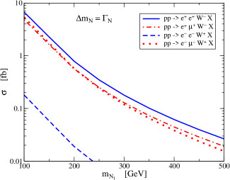
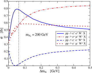
Figure 8: Cross sections for LNV signals in scenario (S2).

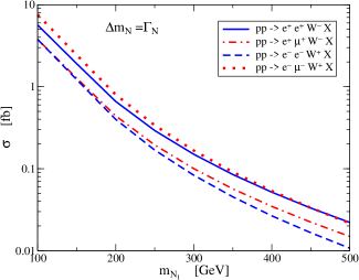
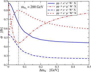
Figure 9: Cross sections for LNV signals in scenario (S3). CP asymmetries are only present for this scenario between signals with different flavour final state charged leptons.

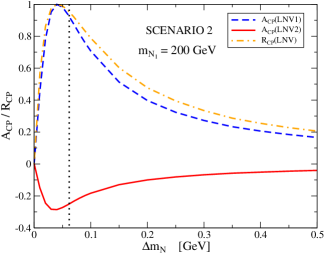
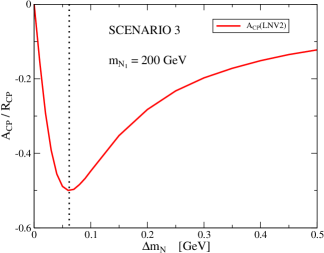
Figure 10: The CP-violating observables $A_{\rm CP}(\rm LNV1)$, $A_{\rm CP}(\rm LNV2)$ and $R_{\rm CP}({\rm LNV})$ as defined in (6.10)–(6.12). In scenario (S3), $A_{\rm CP}(\rm LNV1)=0$ and so $R_{\rm CP}({\rm LNV})=-A_{\rm CP}(\rm LNV2)$.

Table 1: Properties of the cross sections and CP asymmetries considered in Section 6

Observable(s)	Heavy Neutrino	CP violation	CP violation	$K$-dependence
	Type	in (S2)	in (S3)
$\sigma(pp\to e^{\pm}\mu^{\mp}W^{\pm}X)$	Dirac	No	Yes	No
$\sigma(pp\to e^{\pm}\mu^{\mp}W^{\pm}X)$	Majorana	Yes	Yes	No
$\sigma(pp\to e^{\pm}\mu^{\mp}W^{\mp}X)$	Dirac	No	Yes	No
$\sigma(pp\to e^{\pm}\mu^{\mp}W^{\mp}X)$	Majorana	Yes	Yes	No
$\sigma(pp\to e^{\pm}e^{\pm}W^{\mp}X)$	Majorana	Yes	No	No
$\sigma(pp\to\mu^{\pm}\mu^{\pm}W^{\mp}X)$	Majorana	No	No	No
$\sigma(pp\to e^{\pm}\mu^{\pm}W^{\mp}X)$	Majorana	Yes	Yes	No
$A_{\rm CP}({\rm LNC})$	Dirac	No	Yes	No
$A_{\rm CP}({\rm LNC})$	Majorana	Yes	Yes	No
$R_{\rm CP}({\rm LNC})$	Dirac	No	Yes	No
$R_{\rm CP}({\rm LNC})$	Majorana	Yes	Yes	No
$A_{\rm CP}(\rm LNV1)$	Majorana	Yes	No	Yes
$A_{\rm CP}(\rm LNV2)$	Majorana	Yes	Yes	Yes
$R_{\rm CP}({\rm LNV})$	Majorana	Yes	Yes	No

As before, $A_{\rm CP}$ and $R_{\rm CP}$ can be defined as follows:

$$A_{\rm CP}(\rm LNV1) = \frac{\sigma(pp\to e^{+}e^{+}W^{-}X)-K\sigma(pp\to e^{-}e^{-}W^{+}X)}{\sigma(pp\to e^{+}e^{+}W^{-}X)+K\sigma(pp\to e^{-}e^{-}W^{+}X)}\,,$$ (6.10)

$$A_{\rm CP}(\rm LNV2) = \frac{\sigma(pp\to e^{+}\mu^{+}W^{-}X)-K\sigma(pp\to e^{-}\mu^{-}W^{+}X)}{\sigma(pp\to e^{+}\mu^{+}W^{-}X)+K\sigma(pp\to e^{-}\mu^{-}W^{+}X)}\,,$$ (6.11)

$$R_{\rm CP}({\rm LNV}) = \frac{\displaystyle{\frac{\sigma(pp\to e^{+}e^{+}W^{-}X)}{\sigma(pp\to e^{+}\mu^{+}W^{-}X)}-\frac{\sigma(pp\to e^{-}e^{-}W^{+}X)}{\sigma(pp\to e^{-}\mu^{-}W^{+}X)}}}{\displaystyle{\frac{\sigma(pp\to e^{+}e^{+}W^{-}X)}{\sigma(pp\to e^{+}\mu^{+}W^{-}X)}+\frac{\sigma(pp\to e^{-}e^{-}W^{+}X)}{\sigma(pp\to e^{-}\mu^{-}W^{+}X)}}}\,.$$ (6.12)

The signal cross sections given in (6.9) are plotted in the same manner as the LNC signals were. These are shown in Fig. 8 for scenario (S2) and Fig. 9 for scenario (S3). Similarly, the CP-violating observables given in (6.10)–(6.12) are shown in Fig. 10. The cross sections for both the LNC and LNV signals fall very rapidly with increasing heavy neutrino mass. For $|B_{lN}|=0.05$ and an integrated luminosity of 100 fb^-1, to produce at least 10 signal events in any single channel would typically require $m_{N}\lesssim 300-400\,{\rm GeV}$. This could be enough to not just discover heavy neutrinos, but also observe resonant CP violation as well. As can be seen from the plots in Figs. 7 and 10, the CP asymmetries in scenarios (S2) and (S3) are very large for $\Delta m_{N}\approx\Gamma_{N}$. With this condition, and taking $m_{N_{1}}=300\,{\rm GeV}$ for example, scenario (S2) would result in about 20 signal events for $pp\to e^{+}e^{+}W^{-}X$ without a single $pp\to e^{-}e^{-}W^{+}X$ event likely to be observed.

In the limit $\Delta m_{N}=0$, the asymmetries vanish. This is as expected from Section 5.2, since there it is shown that for couplings of equal magnitude, the asymmetries are proportional to the mass-splitting of the heavy neutrinos. For the two CP-violating scenarios considered, the CP asymmetries are larger for Majorana neutrinos than for Dirac ones. However, more examples would need to be calculated to determine if this is a general trend. Since they are constructed out of the asymmetries between two independent processes and their CP-conjugates, it should come as no surprise that the $R_{\rm CP}$ asymmetries are larger than the $A_{\rm CP}$ ones. The one exception to this is $R_{\rm CP}({\rm LNV})$ in scenario (S3). This is because there is no asymmetry between one of the two pairs of CP-conjugate processes it is constructed from. For $\Delta m_{N}=\Gamma_{N}$, both $A_{\rm CP}$ and $R_{\rm CP}$ are independent of the heavy neutrino mass scale, although this is not obvious from our plots since $K$ does depend on $m_{N}$.

7 Conclusions

Based on the resummation formalism developed in [29, 22], we have calculated the $2\times 2$ heavy neutrino propagator matrix for both Dirac and Majorana neutrinos. Our results apply to scenarios for which the two heavy neutrinos that are nearly degenerate in mass dominate the production cross sections. The formalism involves the absorptive part of the heavy neutrino self-energy, which is given to one-loop, again for both Dirac and Majorana neutrinos.

Assuming a two heavy neutrino mixing system, we have given numerical estimates for the production cross sections of LFV and LNV heavy neutrino signal processes at the LHC. These are of the form $pp\to ll^{\prime}WX$, with the final state particle charges (not including the beam remnants $X$) adding up to $\pm 1$. For Dirac neutrinos, the leptons have to have opposite charges and so, in order to avoid large backgrounds, $l$ and $l^{\prime}$ should be different. For Majorana neutrinos, LNV signals of the form $pp\to l^{\pm}l^{\prime\pm}W^{\mp}X$ are also allowed, where $l$ and $l^{\prime}$ can (but do not have to) be equal. The SM background to either of these types of signals should be negligible after cuts. For the magnitudes of couplings we used ($|B_{lN}|=0.05$), heavy neutrinos will be observable at the LHC if they have masses between about $100\,{\rm GeV}$ and about $400\,{\rm GeV}$. If the heavy neutrinos are much lighter than $100\,{\rm GeV}$, the LEP data put severe limits on the $B$-couplings, leading to unobservable signal cross sections.

We have plotted the signal cross sections in three different possible scenarios for the couplings of the heavy neutrinos. In the first, all the couplings are real. This is the CP-conserving limit which is needed to calculate the asymmetry due to the different PDF’s for producing $W^{+}$ and $W^{-}$ bosons. The second and third scenarios are chosen as examples in which large CP asymmetries exist in a number of channels. CP-violating observables constructed from the signal cross sections are also plotted. For a mass-splitting of the two neutrinos of order their widths, these asymmetries can be very large or even maximal, giving rise to resonant CP violation. It should be noted that these scenarios require additional flavour symmetries in the heavy neutrino sector in order to be possible. Experimental constraints, in particular those from the lack of observation of $\mu\to e\gamma$, require contributions from additional particles of new physics (either further heavy neutrinos or something else) to be satisfied. These extra particles would need to cause quite large cancellations in the rate of this process without making a significant contribution to the signals of interest. Also, for Majorana neutrinos, there are theoretical constraints that require at least two additional heavy neutrinos (four in total) to be present in the theory in order to be satisfied. Nevertheless, our results demonstrate that very large CP asymmetries are possible at the LHC. The couplings used have not been motivated in any fashion, but neither are they unique. In particular it should be kept in mind that an interchange of charged lepton labels gives scenarios which are no more or less likely.

Among the different processes we have been studying here, the most realistic modes to look for large CP asymmetries at the LHC are the di-muon or di-electron channels. These processes are LNV and hence are only allowed for Majorana neutrinos. For these channels, it is possible to have the heavy neutrino couplings to either the electron or muon heavily suppressed, hence satisfying the experimental constraints. It may then be possible to have resonant CP violation in these channels without resorting to additional flavour symmetries or cancellations.

The analysis presented here could be extended to other colliders, in particular to the ILC. Here the signals $e^{+}e^{-}\to l^{\pm}W^{\mp}\nu$ can be considered which are CP-conjugates of each other. The ILC should be a cleaner experimental environment and depending on its cms energy, may well be able to produce heavy neutrinos of considerably larger mass. However, the ILC would suffer compared to the LHC in the search for heavy neutrinos in the sense that the SM background cannot so easily be suppressed. Linked to this, evidence of $L$ violation and hence whether or not neutrinos are Majorana particles is far harder to obtain. Also, an observable signal requires a significant coupling of the heavy neutrino to the electron, a requirement not shared by the LHC.

In summary, resonant CP violation due to electroweak-scale heavy neutrinos is an interesting possibility that might well be observed for the first time at the LHC. If realised, this could, in principle, give an explanation for the BAU through resonant leptogenesis. The observation of electroweak-scale heavy neutrinos may not directly unravel the detailed structure of the light neutrino mass matrix, but it will naturally point towards scenarios based on some approximate lepton-number or flavour symmetry (see also our comment in Section 2.1). This approximate lepton-number symmetry may be imprinted into the relative decay rates of the heavy neutrinos into the different charged-lepton flavours $e$, $\mu$ and $\tau$, from which an estimate of the large elements of the Dirac mass matrix $m_{D}$ could, in principle, be obtained. Possible new signatures or constraints from low-energy experiments, including the low-energy neutrino oscillation data, may offer valuable information to restrict the form of $m_{D}$ and the light-to-heavy neutrino-mixing matrix $m_{D}/m_{M}$. A detailed analysis of possible correlations between resonant CP violation due to heavy neutrinos which we have been studying here and other observables may be the subject of a future communication.

Note Added

Shortly after communicating our paper, we became aware of a new analysis of the background contributing to the heavy neutrino signals [68]. According to this analysis, previous studies have grossly underestimated the background by a factor of $\sim 30$, because they did not take into account high-order pile-up processes of jets which cannot be reduced by various kinematic cuts. As a consequence, those authors find that the LHC will be capable of only probing relatively light heavy neutrinos of masses up to 175 GeV, thus restricting the results of our study accordingly. Nonetheless, it should be noticed that the background of high multiplicity jet processes stems predominantly from colour non-singlet states, unlike the 2 distinct jets in the signal which originate from decays of the colourless heavy neutrinos or $W^{\pm}$ bosons. Hence, the signal and background processes are expected to show a different topology of hadronic activities in the central region, which could be used to eliminate the contribution of the high-order pile-up processes of jets, with the hope to extend the reach of the LHC to heavier Majorana neutrinos. Such an analysis lies beyond the scope of this paper.

References

- [1] Super-Kamiokande, Y. Fukuda et al., Phys. Rev. Lett. 81, 1562 (1998), hep-ex/9807003
- [2] CHOOZ, M. Apollonio et al., Phys. Lett. B466, 415 (1999), hep-ex/9907037
- [3] SNO, Q. R. Ahmad et al., Phys. Rev. Lett. 89, 011301 (2002), nucl-ex/0204008
- [4] K2K, M. H. Ahn et al., Phys. Rev. Lett. 90, 041801 (2003), hep-ex/0212007
- [5] KamLAND, K. Eguchi et al., Phys. Rev. Lett. 90, 021802 (2003), hep-ex/0212021
- [6] L3, P. Achard et al., Phys. Lett. B517, 67 (2001), hep-ex/0107014
- [7] A. Pilaftsis, Z. Phys. C55, 275 (1992), hep-ph/9901206
- [8] A. Datta, M. Guchait, and A. Pilaftsis, Phys. Rev. D50, 3195 (1994), hep-ph/9311257
- [9] J. Almeida, F. M. L., Y. A. Coutinho, J. A. Martins Simoes, and M. A. B. do Vale, Phys. Rev. D62, 075004 (2000), hep-ph/0002024
- [10] O. Panella, M. Cannoni, C. Carimalo, and Y. N. Srivastava, Phys. Rev. D65, 035005 (2002), hep-ph/0107308
- [11] T. Han and B. Zhang, Phys. Rev. Lett. 97, 171804 (2006), hep-ph/0604064
- [12] F. del Aguila, J. A. Aguilar-Saavedra, and R. Pittau, J. Phys. Conf. Ser. 53, 506 (2006), hep-ph/0606198
- [13] J. Gluza and M. Zralek, Phys. Rev. D55, 7030 (1997), hep-ph/9612227
- [14] G. Cvetic, C. S. Kim, and C. W. Kim, Phys. Rev. Lett. 82, 4761 (1999), hep-ph/9812525
- [15] J. Almeida, F. M. L., Y. A. Coutinho, J. A. Martins Simoes, and M. A. B. do Vale, Phys. Rev. D63, 075005 (2001), hep-ph/0008201
- [16] F. del Aguila, J. A. Aguilar-Saavedra, A. Martinez de la Ossa, and D. Meloni, Phys. Lett. B613, 170 (2005), hep-ph/0502189
- [17] J. Peressutti, O. A. Sampayo, and J. I. Aranda, Phys. Rev. D64, 073007 (2001), hep-ph/0105162
- [18] S. Bray, J. S. Lee, and A. Pilaftsis, Phys. Lett. B628, 250 (2005), hep-ph/0508077
- [19] M. Flanz, E. A. Paschos, and U. Sarkar, Phys. Lett. B345, 248 (1995), hep-ph/9411366
- [20] M. Flanz, E. A. Paschos, U. Sarkar, and J. Weiss, Phys. Lett. B389, 693 (1996), hep-ph/9607310
- [21] L. Covi, E. Roulet, and F. Vissani, Phys. Lett. B384, 169 (1996), hep-ph/9605319
- [22] A. Pilaftsis, Phys. Rev. D56, 5431 (1997), hep-ph/9707235
- [23] A. Pilaftsis and T. E. J. Underwood, Nucl. Phys. B692, 303 (2004), hep-ph/0309342
- [24] A. Pilaftsis and T. E. J. Underwood, Phys. Rev. D72, 113001 (2005), hep-ph/0506107
- [25] B. Garbrecht, C. Pallis, and A. Pilaftsis, JHEP 12, 038 (2006), hep-ph/0605264
- [26] G. C. Branco, A. J. Buras, S. Jager, S. Uhlig, and A. Weiler, (2006), hep-ph/0609067
- [27] J. Pumplin et al., JHEP 07, 012 (2002), hep-ph/0201195
- [28] A. D. Martin, R. G. Roberts, W. J. Stirling, and R. S. Thorne, Eur. Phys. J. C28, 455 (2003), hep-ph/0211080
- [29] A. Pilaftsis, Nucl. Phys. B504, 61 (1997), hep-ph/9702393
- [30] H. Fritzsch and P. Minkowski, Ann. Phys. 93, 193 (1975)
- [31] P. Minkowski, Phys. Lett. B67, 421 (1977)
- [32] M. Gell-Mann, P. Ramond, and R. Slansky, in Supergravity, edited by P. van Nieuwenhuizen and D. Friedman, p. 315, North-Holland, Amsterdam, 1979
- [33] T. Yanagida, in Preceedings of the Workshop on the Unified Theories and Baryon Number of the Universe, edited by O. Sawada and A. Sugamoto, KEK, Tsukuba, 1979
- [34] R. N. Mohapatra and G. Senjanovic, Phys. Rev. Lett. 44, 912 (1980)
- [35] J. Ellis, M. E. Gomez, and S. Lola, (2006), hep-ph/0612292
- [36] E. Witten, Nucl. Phys. B268, 79 (1986)
- [37] R. N. Mohapatra and J. W. F. Valle, Phys. Rev. D34, 1642 (1986)
- [38] J. Gluza, Acta Phys. Polon. B33, 1735 (2002), hep-ph/0201002
- [39] G. Altarelli and F. Feruglio, New J. Phys. 6, 106 (2004), hep-ph/0405048
- [40] D. Wyler and L. Wolfenstein, Nucl. Phys. B218, 205 (1983)
- [41] S. Nandi and U. Sarkar, Phys. Rev. Lett. 56, 564 (1986)
- [42] J. W. F. Valle, Prog. Part. Nucl. Phys. 26, 91 (1991)
- [43] P. Langacker and D. London, Phys. Rev. D38, 886 (1988)
- [44] B. Pontecorvo, Sov. Phys. JETP 6, 429 (1957)
- [45] B. Pontecorvo, Sov. Phys. JETP 7, 172 (1958)
- [46] Z. Maki, M. Nakagawa, and S. Sakata, Prog. Theor. Phys. 28, 870 (1962)
- [47] T. P. Cheng and L.-F. Li, Phys. Rev. Lett. 45, 1908 (1980)
- [48] J. G. Korner, A. Pilaftsis, and K. Schilcher, Phys. Lett. B300, 381 (1993), hep-ph/9301290
- [49] J. Bernabeu, J. G. Korner, A. Pilaftsis, and K. Schilcher, Phys. Rev. Lett. 71, 2695 (1993), hep-ph/9307295
- [50] C. P. Burgess, S. Godfrey, H. Konig, D. London, and I. Maksymyk, Phys. Rev. D49, 6115 (1994), hep-ph/9312291
- [51] E. Nardi, E. Roulet, and D. Tommasini, Phys. Lett. B327, 319 (1994), hep-ph/9402224
- [52] G. Bhattacharya, P. Kalyniak, and I. Melo, Phys. Rev. D51, 3569 (1995), hep-ph/9503248
- [53] F. Deppisch, T. S. Kosmas, and J. W. F. Valle, Nucl. Phys. B752, 80 (2006), hep-ph/0512360
- [54] A. Ilakovac and A. Pilaftsis, Nucl. Phys. B437, 491 (1995), hep-ph/9403398
- [55] S. Bergmann and A. Kagan, Nucl. Phys. B538, 368 (1999), hep-ph/9803305
- [56] J. I. Illana and T. Riemann, Phys. Rev. D63, 053004 (2001), hep-ph/0010193
- [57] G. Cvetic, C. Dib, C. S. Kim, and J. D. Kim, Phys. Rev. D66, 034008 (2002), hep-ph/0202212
- [58] BABAR, B. Aubert et al., Phys. Rev. Lett. 95, 041802 (2005), hep-ex/0502032
- [59] BABAR, B. Aubert et al., Phys. Rev. Lett. 96, 041801 (2006), hep-ex/0508012
- [60] G. Belanger, F. Boudjema, D. London, and H. Nadeau, Phys. Rev. D53, 6292 (1996), hep-ph/9508317
- [61] J. M. Cornwall and J. Papavassiliou, Phys. Rev. D40, 3474 (1989)
- [62] J. Papavassiliou, Phys. Rev. D41, 3179 (1990)
- [63] D. Binosi and J. Papavassiliou, Phys. Rev. D66, 111901 (2002), hep-ph/0208189
- [64] D. Binosi and J. Papavassiliou, J. Phys. G30, 203 (2004), hep-ph/0301096
- [65] J. Papavassiliou and A. Pilaftsis, Phys. Rev. Lett. 75, 3060 (1995), hep-ph/9506417
- [66] J. Papavassiliou and A. Pilaftsis, Phys. Rev. D53, 2128 (1996), hep-ph/9507246
- [67] J. Papavassiliou and A. Pilaftsis, Phys. Rev. D54, 5315 (1996), hep-ph/9605385
- [68] F. del Aguila, J. A. Aguilar-Saavedra, and R. Pittau, (2007), hep-ph/0703261.