CERN-PH-TH/2007-036

FTUAM 07-03

IFT-UAM/CSIC 07-08

SHEP/07-05

hep-ph/0702286

Neutrino Mixing Sum Rules
and Oscillation Experiments

S. Antusch, P. Huber, S. F. King and T. Schwetz

^a Departamento de Fisica Teórica C-XI and Instituto del Fisica Teórica C-XVI,
Universidad Autónoma de Madrid, Cantoblanco, E-28049 Madrid, Spain
^b Department of Physics, University of Wisconsin,
1150 University Avenue, Madison, WI 53706, USA
^c School of Physics and Astronomy, University of Southampton,
Southampton, SO17 1BJ, UK
^d CERN, Theory Division, Physics Department, CH-1211 Geneva 23, Switzerland

The neutrino mixing sum rule $\theta_{12}-\theta_{13}\cos(\delta)\approx\theta^{\nu}_{12}$ provides a possibility to explore the structure of the neutrino mass matrix in the presence of charged lepton corrections, since it relates the 1-2 mixing angle from the neutrino mass matrix, $\theta_{12}^{\nu}$, to observable parameters of the PMNS mixing matrix. The neutrino mixing sum rule holds if the charged lepton mixing angles are CKM-like, i.e., small and dominated by a 1-2 mixing, and for small 1-3 mixing in the neutrino mass matrix. These conditions hold in a wide class of well motivated flavour models. We apply this sum rule to present oscillation data, and we investigate the prospects of future neutrino facilities for exploring the sum rule by simulating various setups for long-baseline reactor and accelerator experiments. As explicit examples, we use the sum rule to test the hypotheses of tri-bimaximal and bimaximal neutrino mixing, where $\theta^{\nu}_{12}$ is predicted by $\sin^{2}(\theta^{\nu}_{12})=1/3$ or $1/2$, respectively, although the neutrino mixing sum rule can be used to test any prediction for $\theta^{\nu}_{12}$.

1 Introduction

Many attractive classes of models of fermion masses and mixing lead to interesting predictions for the neutrino mass matrix $m_{\nu}$, such as for instance tri-bimaximal or bimaximal mixing. However, the experimentally accessible quantity is the product $U_{\mathrm{PMNS}}=V_{e_{\mathrm{L}}}V^{\dagger}_{\nu_{\mathrm{L}}}$. It includes the neutrino mixing matrix $V_{\nu_{\mathrm{L}}}$, which diagonalizes $m_{\nu}$, and the charged lepton mixing matrix $V_{e_{\mathrm{L}}}$, which diagonalizes the charged lepton mass matrix $M_{e}$. Often, the essential predictions of flavour models are hidden due to the presence of the charged lepton corrections.

Remarkably, in many cases it can be shown that a combination of the measurable PMNS parameters $\theta_{12}$, $\theta_{13}$ and $\delta$ sums up to the theoretically predicted value for the 1-2 mixing of the neutrino mass matrix. For example, in an SO(3) family symmetry model based on the see-saw mechanism with sequential dominance, predicting tri-bimaximal neutrino mixing via vacuum alignment, the neutrino mixing sum rule which is the subject of this paper was first observed in the first paper of Ref. [1]. In the second and third papers of Ref. [1], it was shown that this neutrino mixing sum rule is not limited to one particular model, but applies under very general assumptions, to be specified below. For general 1-2 mixing $\theta^{\nu}_{12}$ of the neutrino mass matrix, the neutrino mixing sum rule of interest here was given as [1]:

$$\theta_{12}-\theta_{13}\cos(\delta) \approx \theta^{\nu}_{12}\;,$$ (1)

in the standard PDG parameterization of the PMNS matrix [2]. The specific neutrino mixing sum rules for tri-bimaximal [3] and bimaximal [4] neutrino mixing are obtained by replacing $\theta^{\nu}_{12}$ by its predictions $\arcsin(\tfrac{1}{\sqrt{3}})\approx 35.3^{\circ}$ and $\tfrac{\pi}{4}=45^{\circ}$, respectively.

Let us note at this point that corrections to neutrino mixing angles from the charged lepton sector have been addressed in various previous studies. Since some of them are sometimes also referred to as “sum rules”, we would like to comment on the differences to the neutrino mixing sum rule of Eq. (1) [1]. For instance, in many works, it has been noticed that charged lepton corrections can make bimaximal neutrino mixing compatible with experimental data [5, 6, 7, 8]. However, in most studies in the literature (e.g. in Ref. [5]), CP phases have been ignored. In other works, where complex mixing matrices were considered, the connection to the experimentally measurable Dirac CP phase $\delta$ has not been identified [6]. For instance, in Ref. [7] in Eq. (25), the correction is related to a phase $\phi$, which is not identical to $\delta$. The introduction of the measurable quantity $J_{CP}$ in this equation leads to a sign ambiguity in their “sum rule”. We would like to remark that various parameterizations of the PMNS matrix are customary, and that it is important to specify unequivocally which convention is used. Assuming standard PDG parameterization of the PMNS matrix [2] where not stated otherwise, the relations of Ref. [8] for bimaximal neutrino mixing are physically inequivalent to the sumrule in Eq. (1) [1]. Equations for corrections to tri-bimaximal neutrino mixing as well as for general $\theta^{\nu}_{12}$ have been considered [9, 10], however the connection to the measurable CP phases has not been established. Finally, CKM-like corrections to neutrino mixing angles have been considered, and called “sum rules”, in Ref. [11], however CP phases have been ignored. In the following, we will simply refer to the formula of Eq. (1) [1] as the sum rule.

In this paper, after deriving the sum rule [1], we investigate how well the combination of parameters on the left-hand of Eq. (1) can be determined in present and future neutrino oscillation facilities, and then compare to the predictions for the right-hand side coming from bi-maximal and tri-bimaximal neutrino mixing. Such a study is interesting since the sum rule of Eq. (1) [1] provides a means of exploring the structure of the neutrino mass matrix in the presence of charged lepton corrections, and enables whole classes of models of neutrino masses and mixings to be tested. However, exploring the sum rule requires to measure the currently undetermined mixing angle $\theta_{13}$ as well as the CP violating phase $\delta$, which is experimentally challenging, as we shall discuss.

The outline of the remainder of the paper is as follows. In Sec. 2 we present for the first time a parameterization-independent derivation of a family of neutrino mixing sum rules, and subsequently show that one of them leads to the sum rule in Eq. (1), using the standard PDG parameterization [2] of the PMNS mixing matrix. After this derivation of the sum rule, and detailed discussion of the conditions of its validity, we then apply it to present oscillation data in Sec. 3. Sec. 4 is devoted to the simulation of future experiments including long-baseline reactor experiments, various second generation superbeam setups, a $\beta$-beam, and neutrino factories. We summarize in Sec. 5.

2 Derivation of the Sum Rule

The mixing matrix in the lepton sector, the PMNS matrix $U_{\mathrm{PMNS}}$, is defined as the matrix which appears in the electroweak coupling to the $W$ bosons expressed in terms of lepton mass eigenstates. With the mass matrices of charged leptons $M_{\mathrm{e}}$ and neutrinos $m_{\nu}$ written as

$${\cal L}=-\bar{e}_{L}M_{\mathrm{e}}e_{R}-\tfrac{1}{2}\bar{\nu}_{L}m_{\nu}\nu_{\mathrm{L}}^{c}+\text{H.c.}\;,$$ (2)

and performing the transformation from flavour to mass basis by

$$V_{\mathrm{e}_{\mathrm{L}}}\,M_{\mathrm{e}}\,V^{\dagger}_{\mathrm{e}_{\mathrm{R}}}=\mbox{diag}(m_{e},m_{\mu},m_{\tau}),\quad V_{\nu_{\mathrm{L}}}\,m_{\nu}\,V^{T}_{\nu_{\mathrm{L}}}=\mbox{diag}(m_{1},m_{2},m_{3}),$$ (3)

the PMNS matrix is given by

$$U_{\mathrm{PMNS}}=V_{e_{\mathrm{L}}}V^{\dagger}_{\nu_{\mathrm{L}}}\,.$$ (4)

Here it is assumed implicitly that unphysical phases are removed by field redefinitions, and $U_{\mathrm{PMNS}}$ contains one Dirac phase and two Majorana phases. The latter are physical only in the case of Majorana neutrinos, for Dirac neutrinos the two Majorana phases can be absorbed as well.

Many attractive classes of models lead to interesting predictions for the neutrino mass matrix $m_{\nu}$, such as for instance tri-bimaximal [3] or bimaximal [4] mixing where $V^{\dagger}_{\nu_{\mathrm{L}}}$ takes the forms

$$V^{\dagger}_{\nu_{\mathrm{L}},\mathrm{tri}}=\left(\begin{array}[]{ccc}\!\sqrt{2/3}&1/\sqrt{3}&0\!\\ \!-1/\sqrt{6}&1/\sqrt{3}&1/\sqrt{2}\!\\ \!1/\sqrt{6}&-1/\sqrt{3}&1/\sqrt{2}\!\end{array}\right)\;\mbox{or}\;\;V^{\dagger}_{\nu_{\mathrm{L}},\mathrm{bi}}=\left(\begin{array}[]{ccc}\!1/\sqrt{2}&1/\sqrt{2}&0\!\\ \!-1/2&1/2&1/\sqrt{2}\!\\ \!1/2&-1/2&1/\sqrt{2}\!\end{array}\right),$$ (11)

respectively, although the sum rule is not necessarily restricted to either of these two forms. As mentioned in the introduction such predictions are not directly experimentally accessible because of the presence of the charged lepton corrections. However, this challenge can be overcome when we make the additional assumption that the charged lepton mixing matrix has a CKM-like structure, in the sense that $V_{e_{\mathrm{L}}}$ is dominated by a 1-2 mixing, i.e. that its elements $(V_{e_{\mathrm{L}}})_{13}$, $(V_{e_{\mathrm{L}}})_{23}$, $(V_{e_{\mathrm{L}}})_{31}$ and $(V_{e_{\mathrm{L}}})_{32}$ are very small compared to $(V_{e_{\mathrm{L}}})_{ij}$ ($i,j=1,2$). In the following simplified derivation, we shall take these elements to be approximately zero, i.e.

$$V_{e_{\mathrm{L}}}\approx\left(\begin{array}[]{ccc}\!(V_{e_{\mathrm{L}}})_{11}&(V_{e_{\mathrm{L}}})_{12}&0\!\\ \!(V_{e_{\mathrm{L}}})_{21}&(V_{e_{\mathrm{L}}})_{22}&0\!\\ \!0&0&1\!\end{array}\right),$$ (15)

and later on comment on the effect of them being non-zero (see footnote 5). For a derivation including these elements, see [12]. This situation arises in many generic classes of flavour models in the context of unified theories of fundamental interactions, where quarks and leptons are joined in representations of the unified gauge symmetries [1, 13].

Under this assumption, it follows directly from Eq. (4) that $(U_{\mathrm{PMNS}})_{31}$, $(U_{\mathrm{PMNS}})_{32}$ and $(U_{\mathrm{PMNS}})_{33}$ are independent of $V_{e_{\mathrm{L}}}$, and depend only on the diagonalization matrix $V^{\dagger}_{\nu_{\mathrm{L}}}$ of the neutrino mass matrix. This leads to the parameterization-independent sum rules which we give in this form for the first time:

$$|(V^{\dagger}_{\nu_{\mathrm{L}}})_{31}| \approx |(U_{\mathrm{PMNS}})_{31}|\;,$$ (16a)

$$|(V^{\dagger}_{\nu_{\mathrm{L}}})_{32}| \approx |(U_{\mathrm{PMNS}})_{32}|\;,$$ (16b)

$$|(V^{\dagger}_{\nu_{\mathrm{L}}})_{33}| \approx |(U_{\mathrm{PMNS}})_{33}|\;.$$ (16c)

These innocuous looking relations enable powerful tests of the structure of the neutrino mass matrix in the presence of charged lepton corrections. Note that the left-hand sides of these relations involve neutrino mixing matrix elements in a particular basis, whereas the right-hand sides are basis invariant quantities. This makes sense in the framework of a flavour theory which has a preferred basis, the so-called “theory basis”.

Let us now study the sum rules in the standard PDG parameterization of the PMNS matrix (see e.g. [2]),

$$U_{\mathrm{PMNS}}=\left(\begin{array}[]{ccc}c_{12}c_{13}&s_{12}c_{13}&s_{13}e^{-\mathrm{i}\delta}\\ -c_{23}s_{12}-s_{13}s_{23}c_{12}e^{\mathrm{i}\delta}&c_{23}c_{12}-s_{13}s_{23}s_{12}e^{\mathrm{i}\delta}&s_{23}c_{13}\\ s_{23}s_{12}-s_{13}c_{23}c_{12}e^{\mathrm{i}\delta}&-s_{23}c_{12}-s_{13}c_{23}s_{12}e^{\mathrm{i}\delta}&c_{23}c_{13}\end{array}\right)\,P_{\mathrm{Maj}}\,,$$ (20)

which is used in most analyses of neutrino oscillation experiments. Here $\delta$ is the so-called Dirac CP violating phase which is in principle measurable in neutrino oscillation experiments, and $P_{\mathrm{Maj}}=\mathrm{diag}(e^{\mathrm{i}\tfrac{\alpha_{1}}{2}},e^{\mathrm{i}\tfrac{\alpha_{2}}{2}},0)$ contains the Majorana phases $\alpha_{1},\alpha_{2}$. In the following we will use this standard parameterization (including additional phases) also for $V^{\dagger}_{\nu_{\mathrm{L}}}$ and denote the corresponding mixing angles by $\theta_{ij}^{\nu}$, while the mixing angles $\theta_{ij}$ without superscript refer to the PMNS matrix.

In addition to the assumption that $V_{e_{\mathrm{L}}}$ is of the form of Eq. (15) we will now assume that the 1-3 mixing in the neutrino mass matrix is negligible,

$$(V^{\dagger}_{\nu_{\mathrm{L}}})_{13}\approx 0\,.$$ (21)

Many textures for the neutrino mass matrix fulfill this relation exactly, for example the cases of bimaximal and tri-bimaximal mixing, although the assumption in Eq. (21) is more general. Using the assumption (21) in the sum rule of Eq. (16a) one obtains

$$s_{23}^{\nu}s_{12}^{\nu}\approx\left|s_{23}s_{12}-s_{13}c_{23}c_{12}e^{\mathrm{i}\delta}\right|\approx s_{23}s_{12}-s_{13}c_{23}c_{12}\cos(\delta)\,,$$ (22)

where the last step holds to leading order in $s_{13}$. Furthermore, Eq. (16c) together with Eq. (21) implies

$$\theta_{23}^{\nu}\approx\theta_{23}+\mathcal{O}(\theta_{13}^{2})\,.$$ (23)

Using this relation in Eq. (22) leads to the sum rule

$$\theta_{12}-\theta_{13}\cot(\theta_{23})\cos(\delta)\approx\theta_{12}^{\nu}\;,$$ (24)

which holds up to first order in $\theta_{13}$. Hence, we have obtained an approximate expression for the (in general unobservable) mixing angle $\theta_{12}^{\nu}$ in terms of directly measurable parameters of the PMNS matrix. This sum rule can be used to test a bimaximal ($\theta^{\nu}_{12}=\tfrac{\pi}{4}$) or tri-bimaximal ($\theta^{\nu}_{12}=\arcsin(\tfrac{1}{\sqrt{3}})$) structure of the neutrino mass matrix, but may as well be applied for a different pattern beyond these two examples. In the following we will specialise our discussion to models predicting maximal 2-3 mixing in the neutrino mass matrix, $\theta_{23}^{\nu}=\tfrac{\pi}{4}$. This includes of course the cases of bimaximal and tri-bimaximal mixing. With Eq. (23) this leads to the sum rule of Eq. (1) [1].

As a side remark we mention that under the above conditions also a simple relation for $|(U_{\mathrm{PMNS}})_{13}|$ can be obtained, $|(U_{\mathrm{PMNS}})_{13}|\approx|(V_{e_{\mathrm{L}}})_{12}|\,|(V^{\dagger}_{\nu_{\mathrm{L}}})_{23}|$. In the standard parameterization it yields

$$\theta_{13}\approx s_{23}\,\theta^{e}_{12}\approx\tfrac{1}{\sqrt{2}}\theta^{e}_{12}\;,$$ (25)

where $|(V_{e_{\mathrm{L}}})_{12}|=\sin(\theta^{e}_{12})\approx\theta^{e}_{12}$, and in the last step we have approximated $\theta_{23}\approx\tfrac{\pi}{4}$. Hence, $\theta_{13}$ is related to the 1-2 mixing in the charged lepton mass matrix. This relation has been noticed by many authors, e.g. Refs. [1, 5, 6, 7, 8, 9, 10, 11, 13], and it can provide additional hints on the underlying theory of flavour (see for example Ref. [1]). Here we will not explore this relation further but focus on the sum rule (1). Note, however, that under the assumptions (15) and (21) the only mixing parameters of the model are $\theta^{e}_{12},\theta_{12}^{\nu},\theta_{23}^{\nu}$, and through the relations (25), (24), (23) all of them can be expressed in terms of measurable PMNS parameters.

Finally, we mention that under the above assumptions Eq. (23) can be used to test predictions for $\theta_{23}^{\nu}$. This is complementary to the application of the sum rule for $\theta_{12}^{\nu}$, and a precise determination of $\theta_{23}$ will allow for an additional test of predictions for the neutrino mass matrix. For the examples of tri-bimaximal and bimaximal neutrino mixing, one can test experimentally the prediction $\theta_{23}\approx\tfrac{\pi}{4}$, in addition to the verification of the corresponding sum rule for $\theta_{12}$. Prospects for the measurement of deviations from maximal 2-3 mixing have been discussed e.g. in Ref. [17].

3 The Sum Rule and Present Oscillation Data

In this section we show that already with present global data from neutrino oscillation experiments the sum rule can be used to test the hypotheses of bimaximal or tri-bimaximal mixing in the neutrino mass matrix. Using the results from the global analysis of Ref. [18] a fit is performed under the assumption of the sum rule Eq. (1) with the constraints $\theta^{\nu}_{12}=45^{\circ}$ for bimaximal mixing or $\theta^{\nu}_{12}=\arcsin(\tfrac{1}{\sqrt{3}})\approx 35.3^{\circ}$ for tri-bimaximal mixing. (See also Ref. [19] for similar considerations.)

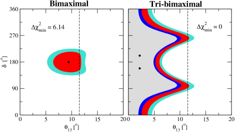
Figure 1: Fit to the present global data on neutrino oscillations under the assumption of the sum rule and bimaximal (left) and tri-bimaximal (right) mixing in the neutrino mass matrix. Allowed regions are shown at 90%, 95%, 99%, 99.73% CL (2 dof) with respect to the unconstrained best fit point. The dashed lines correspond to the upper bound on $\theta_{13}$ at $3\,\sigma$.

Present data implies that $\theta_{12}$ is significantly smaller than $45^{\circ}$, with the upper limit of $39.2^{\circ}$ at $3\,\sigma$ dominated by the SNO solar neutrino experiment [20]. Hence, to reconcile the value $\theta^{\nu}_{12}=45^{\circ}$ for bimaximal mixing one needs a relatively large value of $\theta_{13}$ and $\cos(\delta)\simeq-1$. These expectations are confirmed by the fit, as visible in the left panel of Fig. 1. We obtain $\Delta\chi^{2}_{\mathrm{min}}\approx 6.14$ with respect to the unconstrained best fit point, and hence, allowed regions appear only at 99% and 99.73% CL. Fitting the sum rule for bimaximal mixing requires that both, $\theta_{12}$ and $\theta_{13}$, are pushed towards their upper limits which leads to the increase of $\chi^{2}$ mentioned above. We conclude that already present data disfavours bimaximal neutrino mixing under the assumption of the sum rule at more than $2\sigma$. Hence, either the hypothesis of $\theta_{12}^{\nu}=45^{\circ}$ has to be discarded, or some of the approximations needed for the sum rule are not justified, for instance the charged lepton corrections cannot be of CKM type as assumed in Eq. (15). On the other hand, if the fit is accepted, the sum rule for bimaximal mixing predicts that $\theta_{13}$ is close to its present bound and $\delta\simeq\pi$.

The right panel of Fig. 1 shows the result for the sum rule with tri-bimaximal neutrino mixing. In this case the fit is fully consistent with the data and a best fit point at the same $\chi^{2}$ as the unconstrained fit is found. This follows since the best fit point $\theta_{12}=33.2^{\circ}$ is close to the tri-bimaximal mixing value. Indeed, for small values of $\theta_{13}$, say less than $2^{\circ}$, the sum rule is satisfied within current experimental errors, for all values $\cos(\delta)$. On the other hand, the sum rule leads to a strengthening of the bound on $\theta_{13}$ in the regions where $\cos(\delta)\neq 0$.

4 The Sum Rule and Sensitivities of Future Experiments

In this section we explore the ability of future experiments to constrain the parameter combination $\theta_{12}-\theta_{13}\cos(\delta)$, appearing on the left-hand side of the sum rule in Eq. (1), in order to obtain information on $\theta_{12}^{\nu}$, and so enable a comparison with the predicted values of $\theta_{12}^{\nu}$ coming from particular flavour models. Obviously, in order to do this, the errors on $\theta_{12}$ as well as on $\theta_{13}\cos(\delta)$ should be as small as possible.

Let us first discuss the prospects to improve the accuracy on $\theta_{12}$, which is $4.9^{\circ}$ at $3\,\sigma$ from present data [18], dominated by the SNO solar neutrino experiment [20]. Significant improvement on $\theta_{12}$ can be obtained by long-baseline (LBL) reactor neutrino experiments, similar to the KamLAND experiment [21]. A realistic possibility is that the Super-K experiment will be doped with Gadolinium (SK-Gd) [22]. This will allow for a very efficient detection of reactor $\bar{\nu}_{e}$, and by observing the neutrino flux from the surrounding reactors in Japan a precise determination of the “solar” oscillation parameters will be obtained [23]. Following the analysis of Ref. [24], after 5 years of data taking an accuracy of $4.0^{\circ}$ can be obtained for $\theta_{12}$ at $3\,\sigma$. Another interesting option would be a big scintillator detector such as LENA. In Ref. [24] the possibility of a 44 kt detector installed in the Frejus underground laboratory has been considered. By the observation of the reactor neutrino flux from nearby reactors in France an accuracy of $2.0^{\circ}$ can be obtained for $\theta_{12}$ at $3\,\sigma$ after 5 years of data taking.

Probably the best way to measure $\theta_{12}$ would be a dedicated reactor experiment with only one reactor site at a distance around $60\,\mathrm{km}$ [25, 26], where the first survival probability minimum would be right in the middle of the reactor event rate spectrum. This has been named “SPMIN experiment” in Ref. [26]. The obtainable accuracy in this type of experiment, as in all reactor experiments, is a balance between statistical and systematical errors. The former call for large detectors and powerful reactors, whereas the latter require great experimental skill and a careful design. For illustration we consider here a rather “big” setup corresponding to an exposure of a liquid scintillator detector of 200 GW kt y. The estimated accuracy at $3\,\sigma$ of such an experiment to $\theta_{12}$ is $0.7^{\circ}$ from statistical errors only, and $1.1^{\circ}$ if various systematical effects are taken into account. These numbers have been obtained by applying a similar analysis for the SPMIN experiment as in Ref. [24], where also a detailed description of the various systematics can be found. At such large exposures systematics have a big impact on the accuracy, but it seems difficult to improve the systematics in a very large kiloton sized detector.

	accuracy on $\theta_{12}$ at $3\,\sigma$
present data	$4.9^{\circ}$
SK-Gd, 5 years	$4.0^{\circ}$
LENA @ Frejus, 44 kt, 5 y	$2.0^{\circ}$
SPMIN @ 60 km, 200 GW kt y	$1.1^{\circ}$

Table 1: Accuracy on $\theta_{12}$ from present data and three options for future LBL reactor experiments.

The reason why neither SK-Gd nor LENA at Frejus can compete with a dedicated SPMIN experiment is that many nuclear reactors at various distances contribute which washes out the oscillation signature to some extent. Let us note that also future solar experiments, even with a 1% measurement of the pp-flux, cannot compete with an SPMIN reactor experiment [26]. The prospects of the $\theta_{12}$ measurement are summarized in Tab. 1. In the following combined analysis with LBL accelerator experiments we will consider as reference values the $3\,\sigma$ accuracies of $4.0^{\circ},2.0^{\circ}$ and $1.1^{\circ}$ obtainable at SK-Gd, LENA at Frejus, and a $200\,\mathrm{GW}\,\mathrm{kt}\,\mathrm{y}$ SPMIN experiment, respectively.

Next we turn to the sensitivity of LBL accelerator experiments to the combination of physical parameters appearing on the left-hand side of the sum rule in Eq. (1). These experiments are sensitive to $\delta$ and $\theta_{13}$ but have nearly no sensitivity to $\theta_{12}$. Therefore, we will use the input on $\theta_{12}$ from LBL reactor experiments as described above and perform a combined reactor plus accelerator analysis. We follow the general analysis procedure as described in Ref. [27] with the difference that we now project onto the direction $\theta_{12}-\theta_{13}\cos(\delta)$ in the parameter space. Thus, the obtained results do include the errors and the correlations on $\theta_{13}$ and $\delta$ as well as the errors on $\theta_{12}$, $\Delta m^{2}_{21}$, $\theta_{23}$, $\Delta m^{2}_{31}$ and the matter density. Especially the correlation between $\theta_{13}$ and $\delta$ is crucial, since the relevant oscillation probability contains terms which go as

$$\theta_{13}\sin(\delta)\quad\mathrm{and}\quad\theta_{13}\cos(\delta)\,.$$ (26)

However, the $L/E$-dependence of these two terms is different and hence experiments covering different $L/E$-ranges may have very different sensitivities to $\theta_{13}\cos(\delta)$. For these reasons the accuracy on the combination $\theta_{13}\cos(\delta)$ may be very different from the accuracy individually obtained on $\theta_{13}$ and $\delta$. Therefore, a proper treatment and inclusion of the correlation between $\theta_{13}$ and $\delta$ is mandatory to obtain meaningful results.

For the experiments discussed in the following the sensitivity to either $\theta_{13}\sin(\delta)$ or $\theta_{13}\cos(\delta)$ is dominated by the data from the appearance channels. There are two main reasons for this: The $\sin(\delta)$ term can only appear in off-diagonal transitions, i.e. appearance channels, because it is manifestly CP violating. Secondly, a possible $\cos(\delta)$ contribution in the disappearance channels is always suppressed with respect to the leading $\theta_{23}$ effect and hence plays no statistically significant role. Only for the very largest values of $\theta_{13}$ there is contribution of the disappearance channels, but it is still very small. We will not discuss the possible impact of short baseline reactor experiments which are designed to determine $\theta_{13}$. The reason is, that all the experiments discussed in the following have a superior sensitivity to $\theta_{13}$ on their own.

Setup	Ref.	Baseline	Detector	Beam
SPL	[29]	130 km	440 kt WC	4 MW superbeam, 2 y ($\nu$) + 8 y ($\bar{\nu}$)
T2HK	[29]	295 km	440 kt WC	4 MW superbeam, 2 y ($\nu$) + 8 y ($\bar{\nu}$)
WBB	[30]	1300 km	300 kt WC	1.5 MW superbeam, 5 y ($\nu$) + 5 y ($\bar{\nu}$)
BB350	[32]	730 km	440 kt WC	$5\times 1.1\cdot 10^{18}~{}^{18}$Ne + $5\times 2.9\cdot 10^{18}~{}^{6}$He
NFC	[33]	4000 km	50 kt MID	50 GeV, $4\times 10^{21}~{}\mu^{-}$ + $4\times 10^{21}~{}\mu^{+}$
NFO	[33]	4000+7500 km	2$\times$50 kt MID*	20 GeV, $4\times 10^{21}~{}\mu^{-}$ + $4\times 10^{21}~{}\mu^{+}$

Table 2: Summary of the six future LBL accelerator experiments considered in this study. WC stands for water Čerenkov detector and all masses for this technology are fiducial masses. MID denotes a magnetized iron calorimeter, whereas MID* denotes an improved version thereof. In the column “Beam” we give for BB350 the total number of useful ion decays, and for NFC, NFO the energy of the stored muons and the total number of useful muon decays. For more details see the text.

The calculations are performed with the GLoBES software package [28]. For the input values of the oscillation parameters we use $\Delta m^{2}_{31}=2.5\times 10^{-3}$ eV², $\Delta m^{2}_{21}=8\times 10^{-8}$ eV², $\theta_{23}=45^{\circ}$, and $\theta_{12}=33.2^{\circ}$. We consider six examples for future experiments. Their main characteristics are summarized in Tab. 2. They include three second generation superbeam experiments, SPL – a CERN based experiment with a Mt size water Čerenkov detector at Frejus [29], T2HK, the second stage of the Japanese T2K project [29] (see also Ref. [27]), and WBB – a wide-band beam with a very long baseline as discussed in the US [30, 31]. Furthermore, we consider an advanced $\beta$-beam setup BB350 as described in Ref. [32], with a relativistic $\gamma$-factor of the decaying ¹⁸Ne and ⁶He ions of 350. All these experiment are planed to employ a large water Čerenkov detector with a fiducial mass in the range $300-440$ kt. Note, that the setup labeled WBB assumes an operational time per solar year of $1.7\cdot 10^{7}$ s instead of the usual $10^{7}$ s. The two neutrino factory setups considered here, NFC and NFO are taken from [33]. NFC is what we call conservative, in the sense that it employs only one magnetized iron detector (MID) with the canonical properties regarding muon detection threshold and background rejection [34, 27]. NFO is an optimized version, which uses two identical detectors at two baselines of 4000 km and 7500 km, the latter being the so-called magic baseline [35]. The second difference is that the detector is now an improved MID*, which has a lower muon detection threshold but somewhat larger backgrounds, for details see [33]. The lower threshold allows to reduce the muon energy from 50 GeV to 20 GeV.

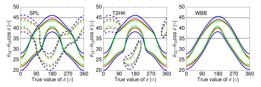
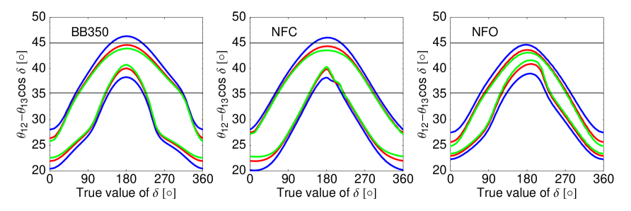
Figure 2: The $3\,\sigma$ allowed interval for the parameter combination $\theta_{12}-\theta_{13}\cos(\delta)$ appearing on the left-hand side of the sum rule in Eq. (1), as a function of the true value of $\delta$ for $\sin^{2}2\theta_{13}=10^{-1}$ from various LBL experiments. The dashed lines correspond to the $\mathrm{sgn}(\Delta m^{2}_{31})$ degenerate solution. The colors indicate different errors on $\theta_{12}$: blue – $4.0^{\circ}$, red – $2.0^{\circ}$ and green – $1.1^{\circ}$ (at $3\,\sigma$). A true value $\sin^{2}\theta_{12}=0.3$ ($\theta_{12}=33.2^{\circ}$) has been assumed. The horizontal lines show the sum rule predictions corresponding to bimaximal and tri-bimaximal neutrino mixing.

Figs. 2 and 3 show the results for the $3\,\sigma$ allowed interval in $\theta_{12}-\theta_{13}\cos(\delta)$ as a function of the true value of $\delta$ assuming $\sin^{2}2\theta_{13}=10^{-1}$ and $10^{-2}$, respectively, from the considered experimental setups. This allowed interval can be compared with theoretical predictions for $\theta_{12}^{\nu}$. We illustrate in the figures the cases of bimaximal and tri-bimaximal mixing by the horizontal lines, but of course any prediction for $\theta_{12}^{\nu}$ can be confronted with the outcome of the experiments. Since we have used as true value for $\theta_{12}$ the present best fit point of $33.2^{\circ}$, bimaximal mixing ($\theta_{12}^{\nu}=45^{\circ}$) can be obtained only for large values of $\theta_{13}$ and $\delta\simeq 180^{\circ}$, in agreement with the discussion in Sec. 3. For larger (smaller) true values of $\theta_{12}$, the bands and islands in Figs. 2 and 3 are shifted up (down) correspondingly.

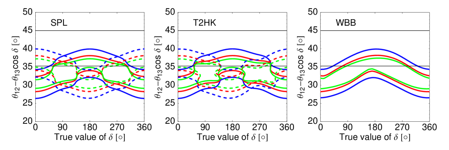
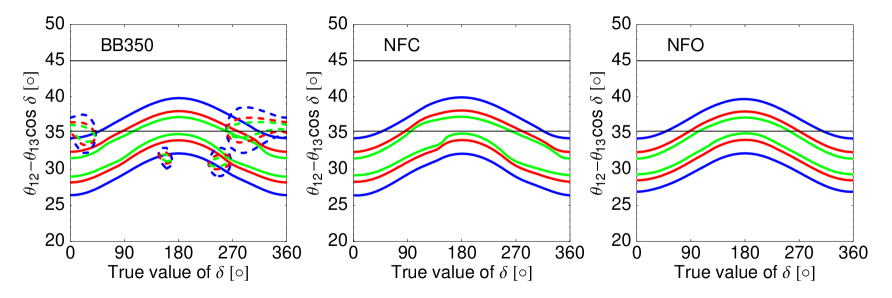
Figure 3: Same as Fig. 2 but for $\sin^{2}2\theta_{13}=10^{-2}$.

All experiments shown in Figs. 2 and 3 have good sensitivity to $\theta_{12}-\theta_{13}\cos(\delta)$. In many cases only some specific values of the CP phase $\delta$ are consistent with a given prediction for $\theta_{12}^{\nu}$, which illustrates the power of the sum rule. An interesting observation is that the presence of the mass hierarchy degenerate solutions (dashed lines) limits the usefulness of SPL and T2HK severely. In these experiments the matter effect is small because of the relatively short baseline. This implies that the mass hierarchy degenerate solution cannot be resolved. Furthermore, the degenerate solution appears at a similar value of $\theta_{13}$ but at a fake CP phase close to $\pi-\delta$ [36]. This changes the sign of the term $\theta_{13}\cos(\delta)$, which explains the shape of the dashed curves in the figures. Because of this degeneracy an ambiguity appears when the sum rule is applied for SPL and T2HK, which significantly limits the possibility to distinguish between various predictions for $\theta_{12}^{\nu}$, especially for large values of $\theta_{13}$ as visible in Fig. 2. A solution to this problem could be the information provided by atmospheric neutrinos in the Mt size detectors used in these experiments [37] (which is not included here). For the other experiments the problem of the degeneracy is absent, since the mass hierarchy degeneracy can be resolved (at sufficiently large $\theta_{13}$) thanks to the longer baselines.

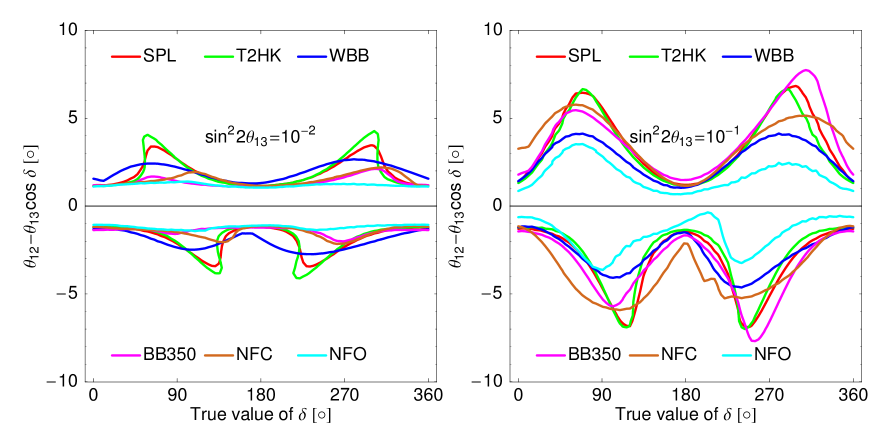
Figure 4: The $3\,\sigma$ error in degrees for the combination of parameters $\theta_{12}-\theta_{13}\cos(\delta)$, appearing on the left-hand side of the sum rule in Eq. (1), as a function of the true value of $\delta$ for $\sin^{2}2\theta_{13}=10^{-2}$ (left) and $\sin^{2}2\theta_{13}=10^{-1}$ (right). The different colored lines are for different experiments as given in the legend. The $\mathrm{sgn}(\Delta m^{2}_{31})$ degenerate solution has been omitted. Although $\sin^{2}\theta_{12}=0.3$ ($\theta_{12}=33.2^{\circ}$) has been used as true value, the results are practically independent of this assumption. The error on $\theta_{12}$ is $1.1^{\circ}$ at $3\,\sigma$.

The performance of all experiments is summarized also in Fig. 4, which shows the obtainable $3\,\sigma$ accuracy for the combination of parameters $\theta_{12}-\theta_{13}\cos(\delta)$, appearing on the left-hand side of the sum rule in Eq. (1), as a function of the true value of $\delta$ for the two cases $\sin^{2}2\theta_{13}=10^{-2}$ and $10^{-1}$. This figure shows that it will be possible to discriminate between models whose predictions for $\theta_{12}^{\nu}$ differ by a few degrees. For the large value of $\theta_{13}$ assumed in Figs. 2 and 4 (right), $\sin^{2}2\theta_{13}=10^{-1}$, the total uncertainty is dominated by the term $\theta_{13}\cos(\delta)$ in the sum rule, and a modest improvement of the current error on $\theta_{12}$ will be enough for exploring the sum rule. The accuracy depends significantly on the true value of $\delta$. Obviously the impact of the term $\theta_{13}\cos(\delta)$ is larger for $|\cos(\delta)|\simeq 1$. For smaller values of $\theta_{13}$ the accuracy on $\theta_{12}$ becomes more important, the overall sensitivity is dominated by the LBL reactor measurement, and the dependence on $\delta$ is weaker.

It follows from Figs. 2, 3, and 4 that NFO has the best performance for all values of $\theta_{13}$, making this the machine of choice for testing the sum rule. NFC compares well to BB350 for this measurement, whereas the performance on $\delta$ and $\theta_{13}$ individually is much worse for NFC than for BB350. The reason for this behaviour is that an experiment whose events are centered around the first oscillation maximum like a $\beta$-beam or superbeam is mainly sensitive to the $\theta_{13}\sin(\delta)$ term. A neutrino factory, however, gets most of its events above the first oscillation maximum and thus is much more sensitive to the $\theta_{13}\cos(\delta)$ term. This explains also the relatively good performance of the WBB visible from the right panel of Fig. 4, where WBB performs second only to NFO. For such large values of $\theta_{13}$ ($\sin^{2}2\theta_{13}=10^{-1}$) spectral information far beyond the first oscillation maximum can be explored efficiently, which is important for constraining $\theta_{13}\cos(\delta)$.

For the somewhat smaller value of $\theta_{13}$, $\sin^{2}2\theta_{13}=10^{-2}$, the performances of NFO, NFC, and BB350 become rather similar, whereas the accuracies obtainable at superbeams depend still to some extent on the true value of $\delta$, see Fig. 4 (left). Note that in this figure the most optimistic accuracy on $\theta_{12}$ from an SPMIN reactor experiment has been assumed, and that the mass hierarchy degeneracy has not been taken into account. Indeed, decreasing the true value of $\theta_{13}$ for all setups besides the neutrino factory one, at some point the mass hierarchy degenerate solution kicks in and introduces an ambiguity in the allowed interval for $\theta_{12}-\theta_{13}\cos(\delta)$, compare also Fig. 3.

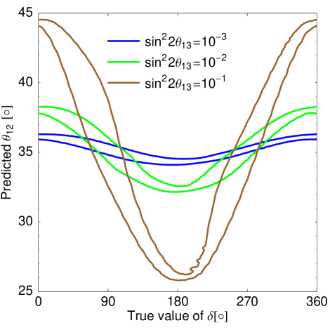
Figure 5: The prediction for $\theta_{12}$ from the sum rule with tri-bimaximal neutrino mixing, as given in Eq.(27). The different curves show the predicted $3\,\sigma$ interval for $\theta_{12}$ following from a NFO measurement of $\theta_{13}\cos(\delta)$ as a function of the true values of $\delta$ and $\theta_{13}$.

For a given model prediction of the neutrino mixing angle $\theta^{\nu}_{12}$, the sum rule in Eq. (1) may be expressed as a prediction for the physical solar mixing angle as a function of the CP violating Dirac oscillation phase $\delta$. Fig. 5 shows the sum rule prediction for the PMNS parameter $\theta_{12}$ corresponding to tri-bimaximal mixing in the neutrino mass matrix, $\theta^{\nu}_{12}=\arcsin(\tfrac{1}{\sqrt{3}})\approx 35.3^{\circ}$, i.e.,

$$\theta_{12}\approx 35.3^{\circ}+\theta_{13}\cos(\delta)\,.$$ (27)

In the figure we have simulated data for the NFO setup for different true values of $\theta_{13}$ and $\delta$ and used Eq. (27) to calculate the resulting $3\,\sigma$ range for the predicted $\theta_{12}$. This result can be compared with the outcome of a separate measurement of $\theta_{12}$ (for example in a reactor experiment) to test whether the hypothesis of tri-bimaximal neutrino mixing is compatible with the assumptions leading to the sum rule.

5 Summary and Conclusions

In this work we have considered the sum rule in Eq. (1), and in particular how well the combination of parameters $\theta_{12}-\theta_{13}\cos(\delta)$, which appears on the left-hand side, can be measured in oscillation experiments. This is important, since the sum rule follows from quite general assumptions which are satisfied in a wide class of flavour models. Moreover, particular such flavour models make definite predictions for $\theta_{12}^{\nu}$, and the sum rule then enables these models to be tested.

We have derived the sum rule, starting from a parameterization independent set of sum rules, which follow from certain well defined assumptions about the nature of charged lepton and neutrino mixings. We then expressed the sum rule in terms of the standard PMNS mixing parameters (see e.g. [2]) commonly used in presenting the results of neutrino oscillation experiments. One way to view the sum rule is to consider the charged lepton corrections to the neutrino mixing angle $\theta_{12}^{\nu}$ predicted from theory, leading to the physical solar neutrino mixing angle $\theta_{12}$. Then, under certain assumptions, the charged lepton correction turns out to only depend on the physical combination $\theta_{13}\cos(\delta)$. To be precise, the sum rule in Eq. (1) holds up to first order in $\theta_{13}$ under the following assumptions:

• The charged lepton mixing matrix is CKM-like, i.e., dominated by the 1-2 mixing angle, see Eq. (15).

• The 1-3 element of the neutrino mixing matrix is negligible, $\theta_{13}^{\nu}\approx 0$.

• The 2-3 mixing in the neutrino mass matrix is maximal, $\theta_{23}^{\nu}\approx 45^{\circ}$, which under the previous two assumptions is equivalent to $\theta_{23}\approx 45^{\circ}+\mathcal{O}(\theta_{13}^{2})$.

If condition (c) is not satisfied and $\theta_{23}$ turns out to be non-maximal the generalized sum rule Eq. (24) has to be used. This would not change the reasoning of this paper, since $\theta_{12}^{\nu}$ still can be expressed only in terms of measurable quantities, involving now also $\theta_{23}$. Hence, condition (c) has been adopted here just for simplicity. Condition (a) holds for a large class of models. For example, in many GUT models the charged lepton mixing matrix is related to the quark mixing matrix since quarks and leptons are joined in representations of the unified gauge symmetries. On the other hand, conditions (b) and (c) are rather typical for flavour models in the neutrino sector. In particular, the popular examples of bimaximal and tri-bimaximal mixing fulfill conditions (b) and (c) exactly.

We have demonstrated the usefulness of the sum rule by imposing it as a constraint in a fit to present global data from neutrino oscillation experiments under the assumptions of bimaximal and tri-bimaximal neutrino mixing. This analysis shows that under the condition (a) bimaximal neutrino mixing is disfavoured at about $2\,\sigma$ by present data with respect to tri-bimaximal mixing, which is perfectly compatible with the data. If the fit for bimaximal mixing is accepted the sum rule predicts that $\theta_{13}$ is close to its present bound and $\delta\simeq\pi$.

In the main part of the paper we have concentrated on the sum rule in the context of future high precision neutrino oscillation experiments. We have considered long-baseline reactor experiments for a precise measurement of $\theta_{12}$, as well as six examples for advanced long-baseline accelerator experiments to constrain the parameter combination $\theta_{13}\cos(\delta)$ appearing in the sum rule. These setups include three options for second generation superbeam experiments, a $\beta$-beam, and two examples for a neutrino factory. It is shown that most of these experiments will allow for a rather precise testing of the sum rule, and $\theta_{12}^{\nu}$ can be inferred within an accuracy of few degrees, where the precise value shows some dependence on the true values of $\theta_{13}$ and $\delta$. For $\sin^{2}2\theta_{13}\lesssim 10^{-2}$ the accuracy is dominated by the error on $\theta_{12}$, whereas for large values of $\theta_{13}$ the precision on the term $\theta_{13}\cos(\delta)$ dominates. Obviously its impact is larger for $|\cos(\delta)|\simeq 1$. Because of the appearance of $\cos(\delta)$ experiments operating not only at the first oscillation maximum (where there is good sensitivity to $\sin(\delta)$) are well suited for this kind of measurement, for example a neutrino factory or a wide-band superbeam. Another interesting observation is that the mass hierarchy degeneracy plays an important role. Since this degeneracy introduces an ambiguity in the CP phase $\delta$ its appearance significantly reduces the information on $\theta_{12}^{\nu}$ which can be extracted from the sum rule.

To conclude, the neutrino mixing sum rule considered in this work is a convenient tool to explore the structure of the neutrino mass matrix in the presence of charged lepton corrections, and to test whole classes of models of neutrino masses and mixings. Already applied to present data it is possible to obtain non-trivial statements, whereas with future high precision oscillation experiments a rather accurate testing of models will become possible in the framework of the sum rule.

Acknowledgments

We would like to thank Michal Malinsky for reading the manuscript. The work of S. Antusch was supported by the EU 6th Framework Program MRTN-CT-2004-503369 “The Quest for Unification: Theory Confronts Experiment”. S. F. King and T. Schwetz acknowledge the EU ILIAS project under contract RII3-CT-2004-506222 for support. Computations were performed on facilities supported by the NSF under Grants No. EIA-032078 (GLOW), PHY-0516857 (CMS Reserach Program subcontract from UCLA), and PHY-0533280 (DISUN), and by the WARF.

References

- [1] S. F. King, JHEP 0508 (2005) 105 [arXiv:hep-ph/0506297]; I. Masina, Phys. Lett. B 633 (2006) 134 [arXiv:hep-ph/0508031]; S. Antusch and S. F. King, Phys. Lett. B 631 (2005) 42 [arXiv:hep-ph/0508044].
- [2] W.-M. Yao et al. [Particle Data Group Collaboration], J. Phys. G 33 (2006) 1.
- [3] P. F. Harrison, D. H. Perkins and W. G. Scott, Phys. Lett. B 530 (2002) 167 [arXiv:hep-ph/0202074]. A similar but physically different form was proposed earlier in: L. Wolfenstein, Phys. Rev. D 18 (1978) 958.
- [4] V. D. Barger, S. Pakvasa, T. J. Weiler and K. Whisnant, Phys. Lett. B 437 (1998) 107 [arXiv:hep-ph/9806387].
- [5] See e.g.: T. Ohlsson and G. Seidl, Nucl. Phys. B 643 (2002) 247 [arXiv:hep-ph/0206087]; C. Giunti and M. Tanimoto, Phys. Rev. D 66, 053013 (2002) [arXiv:hep-ph/0207096].
- [6] S. F. King, JHEP 0209 (2002) 011 [arXiv:hep-ph/0204360]; C. Giunti and M. Tanimoto, Phys. Rev. D 66, 113006 (2002) [arXiv:hep-ph/0209169]; P. H. Frampton, S. T. Petcov and W. Rodejohann, Nucl. Phys. B 687 (2004) 31 [arXiv:hep-ph/0401206]; G. Altarelli, F. Feruglio and I. Masina, Nucl. Phys. B 689 (2004) 157 [arXiv:hep-ph/0402155]; A. Romanino, Phys. Rev. D 70, 013003 (2004) [arXiv:hep-ph/0402258].
- [7] K. A. Hochmuth and W. Rodejohann, arXiv:hep-ph/0607103.
- [8] F. Feruglio, Nucl. Phys. Proc. Suppl. 143, 184 (2005) [Nucl. Phys. Proc. Suppl. 145, 225 (2005)] [arXiv:hep-ph/0410131]; Z. Z. Xing, Phys. Lett. B 618 (2005) 141 [arXiv:hep-ph/0503200].
- [9] F. Plentinger and W. Rodejohann, Phys. Lett. B 625 (2005) 264 [arXiv:hep-ph/0507143].
- [10] R. N. Mohapatra and W. Rodejohann, Phys. Rev. D 72 (2005) 053001 [arXiv:hep-ph/0507312].
- [11] T. Ohlsson, Phys. Lett. B 622 (2005) 159 [arXiv:hep-ph/0506094].
- [12] S. Antusch and S. F. King, in [1].
- [13] Further examples of models can, for example, be found in: S. F. King and G. G. Ross, Phys. Lett. B 574 (2003) 239 [arXiv:hep-ph/0307190]; I. de Medeiros Varzielas and G. G. Ross, Nucl. Phys. B 733 (2006) 31 [arXiv:hep-ph/0507176]; I. de Medeiros Varzielas, S. F. King and G. G. Ross, arXiv:hep-ph/0607045; S. F. King and M. Malinsky, JHEP 0611 (2006) 071 [arXiv:hep-ph/0608021]; S. F. King and M. Malinsky, arXiv:hep-ph/0610250.
- [14] S. F. King, in [1].
- [15] S. F. King, arXiv:hep-ph/0610239.
- [16] S. Antusch, J. Kersten, M. Lindner, M. Ratz and M. A. Schmidt, JHEP 0503 (2005) 024 [arXiv:hep-ph/0501272].
- [17] S. Antusch, P. Huber, J. Kersten, T. Schwetz and W. Winter, Phys. Rev. D 70 (2004) 097302 [arXiv:hep-ph/0404268].
- [18] M. Maltoni, T. Schwetz, M. A. Tortola and J. W. F. Valle, New J. Phys. 6 (2004) 122, for an update see arXiv:hep-ph/0405172 v5; T. Schwetz, Phys. Scripta T127, 1 (2006) [arXiv:hep-ph/0606060].
- [19] I. Masina, in [1].
- [20] S. N. Ahmed et al. [SNO Collaboration], Phys. Rev. Lett. 92 (2004) 181301 [arXiv:nucl-ex/0309004].
- [21] T. Araki et al. [KamLAND Collaboration], Phys. Rev. Lett. 94, 081801 (2005) [arXiv:hep-ex/0406035].
- [22] J. F. Beacom and M. R. Vagins, Phys. Rev. Lett. 93, 171101 (2004) [arXiv:hep-ph/0309300].
- [23] S. Choubey and S. T. Petcov, Phys. Lett. B 594 (2004) 333 [arXiv:hep-ph/0404103].
- [24] S. T. Petcov and T. Schwetz, Phys. Lett. B 642 (2006) 487 [arXiv:hep-ph/0607155].
- [25] H. Minakata, H. Nunokawa, W. J. C. Teves and R. Zukanovich Funchal, Phys. Rev. D 71, 013005 (2005) [arXiv:hep-ph/0407326].
- [26] A. Bandyopadhyay, S. Choubey, S. Goswami and S. T. Petcov, Phys. Rev. D 72 (2005) 033013 [arXiv:hep-ph/0410283].
- [27] P. Huber, M. Lindner and W. Winter, Nucl. Phys. B 645 (2002) 3 [arXiv:hep-ph/0204352].
- [28] P. Huber, M. Lindner and W. Winter, Comput. Phys. Commun. 167, 195 (2005) [arXiv:hep-ph/0407333].
- [29] J. E. Campagne, M. Maltoni, M. Mezzetto and T. Schwetz, arXiv:hep-ph/0603172.
- [30] V. Barger et al., Phys. Rev. D 74, 073004 (2006) [arXiv:hep-ph/0607177].
- [31] M. V. Diwan et al., Phys. Rev. D 68 (2003) 012002 [arXiv:hep-ph/0303081].
- [32] J. Burguet-Castell, D. Casper, E. Couce, J. J. Gomez-Cadenas and P. Hernandez, Nucl. Phys. B 725, 306 (2005) [arXiv:hep-ph/0503021].
- [33] P. Huber, M. Lindner, M. Rolinec and W. Winter, Phys. Rev. D 74 (2006) 073003 [arXiv:hep-ph/0606119].
- [34] A. Cervera, F. Dydak and J. Gomez Cadenas, Nucl. Instrum. Meth. A 451 (2000) 123.
- [35] P. Huber and W. Winter, Phys. Rev. D 68, 037301 (2003) [arXiv:hep-ph/0301257].
- [36] H. Minakata and H. Nunokawa, JHEP 0110 (2001) 001 [arXiv:hep-ph/0108085].
- [37] P. Huber, M. Maltoni and T. Schwetz, Phys. Rev. D 71, 053006 (2005) [arXiv:hep-ph/0501037].