Combining Left-Right And Quark-Lepton Symmetries In 5D

Abstract

A five dimensional model containing both left-right and quark-lepton symmetries is constructed, with the gauge group broken by a combination of orbifold compactification and the Higgs mechanism. An analysis of the gauge and scalar sectors is performed and it is shown that the 5d model admits a simpler scalar sector. Bounds on the relevant symmetry breaking scales are obtained and reveal that two neutral gauge bosons may appear in the TeV energy range to be explored by the LHC. Split fermions are employed to remove the mass relations implied by the quark-lepton symmetry and the necessary fermion localisation is achieved by introducing bulk scalars with kink vacuum profiles. The symmetries of the model constrain the Yukawa sector, which in turn severely constrains the extent to which realistic split fermion scenarios may be realized in the absence of Yukawa coupling hierarchies. Nevertheless we present two interesting one generation constructs. One of these provides a rationale for $m_{t}>m_{b},m_{\tau}$ and $m_{\nu}\ll m_{t}$ with Yukawa parameters which vary by only a factor of five. The other also suppresses the proton decay rate by spatially separating quarks and leptons but requires a Yukawa parameter hierarchy of order $10^{2}$.

I Introduction

Whilst the Standard Model (SM) of particle physics is a very successful theory, it must be admitted that the fermionic sector of the model contains a rather strange set of gauge group representations. One of the triumphs of the SM is the fact that this set of fermion representations conspires to ensure the model is free from both gauge and global anomalies. Though anomaly cancellation provides a very strong motivation for the necessity of the observed representations, it does not provide any insight into their origin. Many questions remain, including ‘Why are left-chiral fermions distinguished from right-chiral fermions?’, ‘Why are quarks and leptons different?’ and ‘What is the origin of the strange set of hypercharge values?’.

The Left-Right (LR) Mohapatra:1986uf and Quark-Lepton (QL) Foot:1990dw symmetric models were introduced in an effort to answer these questions; the hope being that the somewhat awkward arrangement of fermions found in the SM may be simplified by a more fundamental theory possessing a larger degree of symmetry. Both the LR and QL models simplify the structure of the SM fermion representations by relating previously disparate fields. However it is not until these symmetries are combined together in the so called Quark-Lepton Left-Right (QLLR) symmetric model that the fermionic sector of the SM simplifies dramatically. Indeed with both QL and LR symmetries the assumed existence of one SM field mandates the existence of all other SM fields from the same generation Foot:1989wt ; Foot:1991fk .

The goal of Grand Unified Theories (GUTs) is to unite the SM forces into one larger gauge group and reduce the number of independent fermion representations. It is a remarkable feature of the QLLR model that the quantum numbers of quarks and leptons may be unified independent of gauge unification. This interesting fact makes it possible that fermionic unification may be observed at low (TeV) energies even if gauge unification does not occur until a very large energy scale.

A standard problem which arises when one extends the SM to obtain a greater degree of symmetry is that the symmetry breaking sector of the model must also be extended. This issue is often coupled with the method of mass generation in the neutrino sector, with one stage of high energy symmetry breaking assumed to result from a scalar field which possesses the quantum numbers necessary to couple to a right-chiral neutrino Majorana bilinear. Both the $SU(2)_{R}$ scalar triplet in the LR model and the leptonic colour $[SU(3)_{l}]$ sextet scalar in the QL model serve the dual purpose of partially breaking the gauge symmetry and generating a large right-chiral neutrino Majorana mass.

This has the desirable consequence of allowing the see-saw mechanism to be implemented, but at the expense of introducing scalars which do not transform as a fundamental representation of the gauge group. The problem becomes even more severe in the QLLR model; one introduces seventy two additional complex scalar degrees of freedom in the form of gauge representations which transform as chiral $SU(2)$ triplets and colour $SU(3)$ sextets. The QLLR symmetry ensures that once one assumes the existence of a scalar which induces a right-chiral neutrino Majorana mass three additional scalar multiplets are also required.

The large interest in extra dimensional models in recent years has uncovered new mechanisms to achieve symmetry breaking. Using orbifold symmetry reduction allows one to reduce the bulk symmetry to some subgroup operative at low energies (or the zero mode level). This can reduce the number of scalars required in a model and thus simplify the symmetry breaking sector. However the removal of scalars (and in particular the reduction of the SM cutoff in models which seek to solve the hierarchy problem) often removes the see-saw mechanism as a viable source of neutrino mass suppression.

Fortunately the inclusion of additional spatial dimensions permits new mechanisms for suppressing neutrino masses. In particular split fermions allow one to suppress fermion masses relative to the electroweak scale by spatially separating left- and right-chiral fermions in an additional dimension Arkani-Hamed:1999dc . The subsequent reduction in higher dimensional wave function overlap serves to suppress the effective Yukawa coupling constants in the 4d theory.

In this work we investigate the implementation of these two mechanisms in the context of a QLLR model. The objective of our paper is to retain the attractive fermionic unification found in QLLR models but reduce the complicated symmetry breaking sector required in 4d constructs. We find that the scalar sector of the model may be significantly reduced in 5d with the seventy degrees of freedom previously mentioned not required to achieve a realistic low energy model. The symmetry breaking sector of our model has the additional consequence of permitting the two exotic neutral gauge bosons found in QLLR models, $Z^{\prime}$ and $Z^{\prime\prime}$, to appear at TeV energies and thus be observable at the LHC. Previous works have all required one of these bosons to be unobservably heavy.

The use of split fermions has a number of interesting consequences. We provide two distinct one generational constructs that suppress neutrino masses to experimentally acceptable values and also provide a rationale for the inequalities $m_{t}>m_{b},m_{\tau}$. However the large degree of symmetry in the model severely constrains the Yukawa sectors and it is a non-trivial task to obtain fermion localisation patterns which account for the range of fermion masses observed and remove the need for Yukawa parameter hierarchies.

We show that one generation of flavour can be accounted for with Yukawa parameters which vary only by a factor of five. However this setup does not allow one to suppress proton decay by spatially separating quarks and leptons and thus, along with the majority of split fermion works completed to date, the model must be extended to avoid the usual hierarchy problem associated with stabilizing the electroweak scale. In the alternative construct the proton decay rate is safely suppressed by separating quarks and leptons, but a Yukawa hierarchy of order $10^{2}$ is necessary to achieve one generation of flavour. Thus one may alleviate the hierarchy problem by lowering the cutoff to order 100 TeV. Further work is required to see if these promising results can be carried over to a full three generation model.

We note that recent works have investigated the LR model Mimura:2002te ; Mohapatra:2002rn ; Perez:2002wb and the QL model McDonald:2006dy ; Coulthurst:2006kz ; Coulthurst:2006zu in 5d. The concept of leptonic colour has also been generalised in Foot:2006ie and studied within the context of unified theories in Joshi:1991yn ; Babu:2003nw ; Chen:2004jz ; Demaria:2005gk ; Demaria:2006uu ; Demaria:2006bd .

The layout of this paper is as follows. In Section II we review the main features of the QLLR model. Section III details the symmetry breaking sector of our 5d construct and Section IV looks at the gauge sector. The fermionic sector is detailed in Section V, where we briefly describe the features of split fermion models required for our investigations and then present two promising one generation fermionic geographies. In Section VI we discuss neutral currents and derive bounds on the symmetry breaking scales of the model. We consider some experimental signatures of the model in Section VII and conclude in Section VIII.

II Review Of The Quark-Lepton Left-Right Symmetric Model

In this section we review the four dimensional QLLR model Foot:1989wt ; Foot:1991fk . To this end, let us recall some features of the SM, the LR model and the QL model. The fermion spectrum of the SM is given by:

$$Q_{L}\sim(3,2,1/3),\mkern 8.0muu_{R}\sim(3,1,4/3),\mkern 8.0mud_{R}\sim(3,1,-2/3),$$

(1)

$$L_{L}\sim(1,2,-1),\mkern 8.0mue_{R}\sim(1,1,-2),$$

where we have suppressed generational indices and the quantum numbers label the transformation properties of the fields under $G_{SM}\equiv SU(3)_{c}\otimes SU(2)_{L}\otimes U(1)_{Y}$. Whilst GUTs provide us with a candidate explanation for the origin of the SM fermion quantum numbers, it is safe to say that we do not yet know the underlying theory responsible for the rather curious collection of quantum numbers in (II). The key observation made in GUTs is that the SM quantum numbers may be understood if one embeds the group $G_{SM}$ into a simple group $H$. The SM fermions are embedded into one (or two in the case of $SU(5)$) representation $R$ of $H$. By employing a suitable symmetry breaking mechanism to reduce the symmetry operative at observable energy scales from the unifying group $H$ down to $G_{SM}$, the SM fermion quantum numbers may be understood in terms of the decomposition of $R$ under the low energy group $G_{SM}$.

An alternative approach employed to uncover candidate extensions of the SM follows from the observation that there exist suggestive similarities amongst the quantum numbers of the SM fermions. One similarity is that all left- and right-chiral fields possess identical electric and colour charges; another is the similar family structure of quarks and leptons, with all left-chiral fields forming $SU(2)_{L}$ doublets whilst their right-chiral partners assume singlet $SU(2)_{L}$ representations.

The motivation for the LR and QL models arises from these observed similarities. By positing that the observed similarity between left- and right-handed fields is the result of an underlying symmetry one is lead to the LR model Mohapatra:1986uf . This requires one to increase the fermion content of the SM to include $\nu_{R}$ and to extend the gauge group from $G_{SM}$ to $G_{LR}\equiv SU(3)_{c}\otimes SU(2)_{L}\otimes SU(2)_{R}\otimes U(1)_{B-L}$. This extension has the desirable consequence of simplifying the structure of the SM fermion content. The fermion spectrum of the LR model is:

$$Q_{L}\sim(3,2,1,1/3),\mkern 20.0muQ_{R}\sim(3,1,2,1/3),$$

(2)

$$L_{L}\sim(1,2,1,-1),\mkern 20.0muL_{R}\sim(1,1,2,-1),$$

and the LR model Lagrangian is taken to be invariant under a discrete $Z_{2}$ symmetry, which we label as $Z_{2}^{LR}$, and whose action is defined by

$$L_{L}\leftrightarrow L_{R},\mkern 10.0muQ_{L}\leftrightarrow Q_{R},\mkern 10.0muW_{L}\leftrightarrow W_{R},$$ (3)

where $W_{L(R)}$ denotes the $SU(2)_{L(R)}$ gauge bosons. Observe that the extended model reduces the total number of fermion representations and also reduces the number of independent $U(1)$ charges per generation from five to two. The group $G_{LR}$ is broken to ensure that $U(1)_{Y}\subset SU(2)_{R}\otimes U(1)_{B-L}$ so that the SM is recovered at low energies.

If one instead focuses on the similar family structures of quarks and leptons in the SM (assuming three $\nu_{R}$s) and follows the same procedure one arrives at the QL model Foot:1990dw . This requires $G_{SM}$ to be extended to $G_{QL}\equiv SU(3)_{l}\otimes SU(3)_{c}\otimes SU(2)_{L}\otimes U(1)_{X}$ where $SU(3)_{l}$ is known as lepton colour and is the leptonic equivalent of $SU(3)_{c}$ in the quark sector. As well as adding $\nu_{R}$ to the SM fermion spectrum one must also triple the number of leptons, giving the fermion spectrum

$$Q_{L}\sim(1,3,2,1/3),\mkern 20.0muL_{L}\sim(3,1,2,-1/3),$$

$$u_{R}\sim(1,3,1,4/3),\mkern 20.0muE_{R}\sim(3,1,1,-4/3),$$ (4)

$$d_{R}\sim(1,3,1,-2/3),\mkern 20.0muN_{R}\sim(3,1,1,2/3).$$

The usual lepton $SU(2)_{L}$ doublet is contained in $L_{L}$ and $e_{R}$ ($\nu_{R}$) is found inside $E_{R}$ ($N_{R}$). The Lagrangian of the QL model permits a discrete symmetry, $Z_{2}^{QL}$, defined as follows:

$$Q_{L}\leftrightarrow L_{L}\mkern 10.0muE_{R}\leftrightarrow u_{R},\mkern 10.0muN_{R}\leftrightarrow d_{R},$$

(5)

$$G_{c}\leftrightarrow G_{l},\mkern 10.0muC\leftrightarrow-C$$

where $G_{c}$ ($G_{l}$) denotes the $SU(3)_{c(l)}$ gauge bosons and $C$ is the $U(1)_{X}$ gauge boson. This model reduces the number of independent $U(1)$ charges relative to the SM and also reduces the number of independent fermion representations per generation from five (in the SM) to three. As with the LR model, the total number of fermions per generation is greater than that of the SM due to the exotics required to permit the defining discrete symmetry of the model.

One may combine the symmetries $Z_{2}^{QL}$ and $Z_{2}^{LR}$ to obtain the QLLR model. The gauge group of this model is

$$G_{QLLR}=SU(3)_{l}\otimes SU(3)_{c}\otimes SU(2)_{L}\otimes SU(2)_{R}\otimes U(1)_{V}$$

and the fermions are assigned to the following representations:

$$L_{L}\sim(3,1,2,1,-1/3),\mkern 17.0muL_{R}\sim(3,1,1,2,-1/3),$$

(6)

$$Q_{L}\sim(1,3,2,1,1/3),\mkern 24.0muQ_{R}\sim(1,3,1,2,1/3).$$

The action of the discrete symmetry $Z_{2}^{QL}\times Z_{2}^{LR}$ is defined as follows

$$\begin{array}[]{ccccccccccc}L_{L}&\leftrightarrow&L_{R}&&V&&G_{l}&&W_{L}&\leftrightarrow&W_{R}\\ \updownarrow&{}\hfil&\updownarrow&&\updownarrow&&\updownarrow&&{}\hfil&{}\hfil&{}\hfil\\ Q_{L}&\leftrightarrow&Q_{R}&&-V&&G_{q}&&{}\hfil&{}\hfil&{}\hfil\end{array}$$ (7)

where the QL (LR) symmetry acts vertically (horizontally) and $V$ denotes the $U(1)_{V}$ boson. Note that (6) contains only one independent fermion field with the quantum numbers of all other fermion fields determined completely by the discrete symmetry. It is interesting that unification of the quark and lepton quantum numbers may be achieved in the QLLR model, independent of gauge coupling unification. This is contrary to the usual expectation that relationships which may exist between the quark and lepton quantum numbers are the manifestation of a symmetry which is operative only at the GUT scale.

The simplified fermion content of the QLLR model comes at the expense of an extended scalar content. Both the $SU(3)_{l}$ and $SU(2)_{R}$ symmetries must be broken to reproduce the SM at low energies. This breaking proceeds in two steps. The first step is achieved by the introduction of the scalars

$$\Delta_{1L}\sim(\bar{6},1,3,1,2/3),\mkern 17.0mu\Delta_{1R}\sim(\bar{6},1,1,3,2/3),$$

(8)

$$\Delta_{2L}\sim(1,\bar{6},3,1,-2/3),\mkern 17.0mu\Delta_{2R}\sim(1,\bar{6},1,3,-2/3),$$

which transform as

$$\begin{array}[]{ccc}\Delta_{1L}&\leftrightarrow&\Delta_{1R}\\ \updownarrow&{}\hfil&\updownarrow\\ \Delta_{2L}&\leftrightarrow&\Delta_{2R}\end{array}$$ (9)

under the discrete symmetries. The Yukawa Lagrangian for these fields is

$$\mathcal{L}_{\Delta} = \lambda_{\Delta}[\overline{(L_{L})^{c}}L_{L}\Delta_{1L}+\overline{(L_{R})^{c}}L_{R}\Delta_{1R}+\overline{(Q_{L})^{c}}Q_{L}\Delta_{2L}$$ (10)

$$\qquad+\overline{(Q_{R})^{c}}Q_{R}\Delta_{2R}]+\mathrm{H.c.},$$

Provided the neutral component of $\Delta_{1R}$ develops a non-zero VEV the gauge symmetry will be broken as per

$$\begin{array}[]{c}G_{QLLR}\\ \downarrow\\ SU(2)_{l}\otimes SU(3)_{c}\otimes SU(2)_{L}\otimes U(1)_{Y}\otimes U(1)_{Y^{\prime}},\end{array}$$

where $Y$ denotes the SM hypercharge, $Y^{\prime}$ denotes some orthogonal unbroken $U(1)$ factor whose precise form will not be important to us and $SU(2)_{l}\subset SU(3)_{l}$. The hypercharge generator is given by

$$Y=2I_{3R}+\frac{1}{\sqrt{3}}T_{l}^{8}+V,$$ (11)

where $T_{l}^{8}=1/\sqrt{3}\times\rm diag(-2,1,1)$ is a diagonal generator of $SU(3)_{l}$ and $I_{3R}=1/2\times\rm diag(1,-1)$ is the diagonal generator of $SU(2)_{R}$. Further symmetry breaking is accomplished by including the usual colour triplet scalars found in QL models, namely

$$\chi_{l}\sim(3,1,1,1,2/3),\mkern 20.0mu\chi_{q}\sim(1,3,1,1,-2/3),$$

which form partners under the $Z_{2}^{QL}$ symmetry, $\chi_{l}\leftrightarrow\chi_{q}$. The Yukawa Lagrangian for these fields is

$$\mathcal{L}_{\chi} = \lambda_{\chi}[\overline{(L_{L})^{c}}L_{L}\chi_{l}+\overline{(L_{R})^{c}}L_{R}\chi_{l}+\overline{(Q_{L})^{c}}Q_{L}\chi_{q}$$ (12)

$$\qquad+\overline{(Q_{R})^{c}}Q_{R}\chi_{q}]+\mathrm{H.c.}.$$

When the electrically neutral component of $\chi_{l}$ develops a VEV the following symmetry breaking occurs

$$\begin{array}[]{c}SU(2)_{l}\otimes SU(3)_{c}\otimes SU(2)_{L}\otimes U(1)_{Y}\otimes U(1)_{Y^{\prime}}\\ \downarrow\\ SU(2)_{l}\otimes SU(3)_{c}\otimes SU(2)_{L}\otimes U(1)_{Y}.\end{array}$$

Note that $SU(2)_{l}$ remains unbroken. Whilst a large number of additional scalars are required to achieve the desired symmetry breaking it should be pointed out that only two additional Yukawa couplings are introduced. The symmetries highly constrain the Yukawa Lagrangian and, though we shall not need to consider it, they also constrain the scalar potential. Let us discuss briefly the spectrum of exotic fermions and gauge bosons expected in the model.

The VEV hierarchy $\langle\Delta_{1R}\rangle\gg\langle\chi_{l}\rangle$ is assumed as the nonzero value for $\langle\Delta_{1R}\rangle$ induces a Majorana mass for the right-handed neutrinos. After neutrinos acquire a Dirac mass at the electroweak symmetry breaking scale the seesaw mechanism will thus be operative to suppress the observed neutrino masses below the electroweak scale. The nonzero VEV for $\langle\Delta_{1R}\rangle$ also gives mass to the $SU(3)_{l}/SU(2)_{l}$ coset gauge bosons and the $W_{R}$ bosons. As the seesaw mechanism requires $\langle\Delta_{1R}\rangle$ to be large, roughly $10^{14}$ GeV, these gauge bosons become unobservably heavy. The VEV for $\Delta_{1R}$ also breaks the linear combination of $I_{3R}$, $T_{l}$ and $V$ which is orthogonal to $Y$ and $Y^{\prime}$. Thus a neutral boson $Z^{\prime\prime}$ gains a mass of order $\langle\Delta_{1R}\rangle$.

The non zero VEV for $\chi_{l}$ breaks $Y^{\prime}$, resulting in a massive neutral gauge boson with an order $\langle\chi_{l}\rangle=w_{l}$ mass. The symmetry breaking induced by $\chi_{l}$ also gives mass to the exotic fermions introduced to fill out the $SU(3)_{l}$ fermion representations. These fermions are known as liptons in the literature and are a common feature of models possessing a QL symmetry. The unbroken $SU(2)_{l}$ symmetry serves to confine the liptons into two-fermion bound states. These states all decay via the usual electroweak interactions into the known fermions Foot:1991fk . The lower bound on $w_{l}$ is of order TeV (we provide a detailed discussion of the bound on $w_{l}$ in Section VI) and the key experimental signatures for the model are the $Z^{\prime}$ boson and the liptons. The liptons may be produced at the LHC via the usual electroweak interactions and via virtual $Z^{\prime}$ creation.

The gauge group $G_{SM}\otimes SU(2)_{l}$ must be broken down to $SU(3)_{c}\otimes U(1)_{Q}\otimes SU(2)_{l}$. This requires the introduction of a Higgs bidoublet

$$\Phi\sim(1,1,2,2,0),$$ (13)

resulting in the following electroweak Yukawa Lagrangian

$$\mathcal{L}_{\Phi} = \lambda_{\Phi 1}[\bar{L}_{L}L_{R}\Phi+\bar{Q}_{L}Q_{R}\tilde{\Phi}]+$$ (14)

$$\lambda_{\Phi 2}[\bar{L}_{L}L_{R}\tilde{\Phi}+\bar{Q}_{L}Q_{R}\Phi]+\mathrm{H.c.},$$

where $\tilde{\Phi}=\epsilon\Phi^{*}\epsilon$ (we denote the two dimensional anti-symmetric tensor as $\epsilon$) and

$$\Phi\leftrightarrow\tilde{\Phi}$$ (15)

under the QL symmetry. If the neutral components of $\Phi$ develop a VEV the desired symmetry breaking is achieved. The Yukawa couplings in (14) give rise to fermion Dirac masses and result in mass relations of the type

$$m_{u}=m_{e},\qquad m_{d}=m_{\nu},$$ (16)

where $m_{\nu}$ is the neutrino Dirac mass. As the light neutrinos acquire mass via the seesaw mechanism the relationship $m_{d}=m_{\nu}$ doesn’t provide any phenomenological difficulty. The right-handed neutrinos acquire a Majorana mass through their couplings to $\Delta_{1R}$ and there is enough parameter freedom in the Lagrangian $\mathcal{L}_{\Delta}$ to ensure that arbitrary neutrino mass values can be obtained. The relationship between the down quark mass matrix and the neutrino Dirac mass matrix actually serves to reduce the number of parameters employed to implement the seesaw mechanism. The mass relations between the electrons and the up quarks may also be removed by introducing an additional bidoublet $\Phi^{\prime}\sim(1,1,2,2,0)$. This doubles the number of Yukawa couplings and thus also nullifies the mass relations $m_{d}=m_{\nu}$, thereby reducing predictivity of the model.

III Symmetry Breaking In Five Dimensions

In this work we study the quark-lepton left-right symmetric extension to the Standard Model in five dimensions. The additional spatial dimension is taken as the orbifold $S^{1}/Z_{2}\times Z_{2}^{\prime}$, whose coordinate is labelled as $y$. The construction of the orbifold proceeds via the identification $y\rightarrow-y$ under the $Z_{2}$ symmetry and $y^{\prime}\rightarrow-y^{\prime}$ under the $Z_{2}^{\prime}$ symmetry, where $y^{\prime}=y+\pi R/2$. The physical region in $y$ is given by the interval $[0,\pi R/2]$.

Given the absence of chirality in five dimensions we shall denote the gauge group of the theory as $SU(3)_{l}\times SU(3)_{c}\times SU(2)_{1}\times SU(2)_{2}\times U(1)_{V}$. We will be required to ensure that the low energy fermion spectrum contains the chiral fermions found in the SM. The zero mode $SU(2)_{1(2)}$ gauge bosons will eventually be identified with the usual $W_{L(R)}$ bosons in LR models via their action on the low energy fermion content. Thus the 5d theory is invariant under the interchange $1\leftrightarrow 2$ which will prove to be equivalent to the usual LR symmetry in the low energy theory. This matter has already been discussed in Mohapatra:2002rn . We shall continue to label the discrete symmetry of the 5d model as $Z_{2}^{QL}\times Z_{2}^{LR}$.

The orbifold action also has a definition on the space of gauge fields which propagate in the bulk. We define $P$ and $P^{\prime}$ to be matrix representations of the orbifold actions $Z_{2}$ and $Z_{2}^{\prime}$ respectively. To maintain gauge invariance under these projections, the gauge fields must have the transformations

$$A_{\mu}(x^{\mu},y) \rightarrow A_{\mu}(x^{\mu},-y)=PA_{\mu}(x^{\mu},y)P^{-1},$$ (17)

$$A_{5}(x^{\mu},y) \rightarrow A_{5}(x^{\mu},-y)=-PA_{5}(x^{\mu},y)P^{-1},$$

$$A_{\mu}(x^{\mu},y^{\prime}) \rightarrow A_{\mu}(x^{\mu},-y^{\prime})=P^{\prime}A_{\mu}(x^{\mu},y^{\prime})P^{\prime-1},$$

$$A_{5}(x^{\mu},y^{\prime}) \rightarrow A_{5}(x^{\mu},-y^{\prime})=-P^{\prime}A_{5}(x^{\mu},y^{\prime})P^{\prime-1},$$

where $A$ denotes the bulk gauge sector,

$$A^{M}(x^{\mu},y) = G^{M}_{l}(x^{\mu},y)\oplus G^{M}_{q}(x^{\mu},y)\oplus W^{M}_{1}(x^{\mu},y)\oplus W^{M}_{2}(x^{\mu},y)\oplus V^{M}(x^{\mu},y),$$ (18)

$$= G_{l}^{M\,a}\,T^{a}\oplus G_{q}^{M\,a}\,T^{a}\oplus W_{1}^{M\,i}\,\tau^{i}\oplus W_{2}^{M\,i}\tau^{i}\oplus V,$$

with $M$ being the 5d Lorentz index, $T$ denotes the $SU(3)$ generators, $\tau$ denotes the $SU(2)$ generators and the gauge indices take the values $a=1,2,...,8$ and $i=1,2,3$.

Given that $P$ and $P^{\prime}$ define a representation of reflection symmetries their eigenvalues are $\pm 1$. We can express these matrices in diagonal form, with a freedom in the parity choice of the entries. The exact nature of these actions then completely determines the gauge symmetry which remains unbroken in the low energy limit of the theory (namely the zero mode gauge sector). Unless $P$ is the identity matrix, not all the gauge fields will commute with the orbifold action. These fields will not possess a zero mode, and thus only a subset of the 5d gauge theory is manifest at the zero mode level. Ideally, the bulk gauge group would reduce to $G_{SM}\otimes SU(2)_{l}$ at the zero mode level; however, this is not directly possible via orbifolding. The $Z_{2}\times Z_{2}^{\prime}$ actions are abelian and commute with the diagonal gauge group generators. Subsequently, the rank of the bulk gauge group must be conserved at the zero mode level. This means that breaking unwanted $SU(3)$ and $SU(2)$ factors has the trade-off of retaining spurious $U(1)$ subgroups and one must invoke a mechanism in tandem to orbifolding in order to accomplish the breaking to $G_{SM}\otimes SU(2)_{l}$.

The orbifold action can be decomposed as:

$$(P,P^{\prime})=$$

$$(P_{l}\oplus P_{q}\oplus P_{1}\oplus P_{2}\oplus P_{V},~{}P^{\prime}_{l}\oplus P^{\prime}_{q}\oplus P^{\prime}_{1}\oplus P^{\prime}_{2}\oplus P^{\prime}_{V}),$$

with

$$P_{l} = \text{diag}(1,1,1),~{}P_{l}^{\prime}=\text{diag}(-1,1,1),$$

$$P_{q} = P_{q}^{\prime}=\text{diag}(1,1,1),$$

$$P_{1} = P_{1}^{\prime}=\text{diag}(1,1),$$

$$P_{2} = \text{diag}(1,1),~{}P_{2}^{\prime}=\text{diag}(-1,1)$$

$$P_{V} = P_{V}^{\prime}=\rm 1.$$ (19)

The only non-trivial entries occur in the $SU(2)_{2}$ and $SU(3)_{l}$ gauge space. Denoting these gauge fields as

$$W_{2}=\frac{1}{2}\left(\begin{array}[]{cc}W_{2}^{0}&\sqrt{2}W_{2}^{+}\\ \sqrt{2}W_{2}^{-}&-W_{2}^{0}\end{array}\right),$$ (20)

and

$$G_{l}=\left(\begin{array}[]{ccc}-\frac{2}{\sqrt{3}}G_{l}^{0}&\sqrt{2}Y_{l}^{1}&\sqrt{2}Y_{l}^{2}\\ \sqrt{2}Y_{l}^{1{\dagger}}&G_{l}^{3}+\frac{1}{\sqrt{3}}G_{l}^{0}&\sqrt{2}\emph{\~{G}}_{l}\\ \sqrt{2}Y_{l}^{2{\dagger}}&\sqrt{2}\emph{\~{G}}_{l}^{{\dagger}}&-G_{l}^{3}+\frac{1}{\sqrt{3}}G_{l}^{0}\end{array}\right),$$ (21)

the $Z_{2}\times Z_{2}^{\prime}$ parities of these fields is found to be

$$G^{0}_{l\mu},~{}G^{3}_{l\mu},~{}\emph{\~{G}}_{l\mu},~{}\emph{\~{G}}^{{\dagger}}_{l\mu},~{}W^{0}_{2\mu}:~{}(+,+),$$ (22)

$$Y^{1}_{l\mu},~{}Y^{2}_{l\mu},~{}Y^{1{\dagger}}_{l\mu},~{}Y^{2{\dagger}}_{l\mu},~{}W^{\pm}_{2\mu}:~{}(+,-),$$ (23)

$$G^{0}_{l5},~{}G^{3}_{l5},~{}\emph{\~{G}}_{l5},~{}\emph{\~{G}}^{{\dagger}}_{l5},~{}W^{0}_{2,5}:~{}(-,-),$$ (24)

$$Y^{1}_{l5},~{}Y^{2}_{l5},~{}Y^{1{\dagger}}_{l5},~{}Y^{2{\dagger}}_{l5},~{}W^{\pm}_{2,5}:~{}(+,-).$$ (25)

A general five dimensional field, $\psi$, can be expanded in terms of Fourier modes in the compact dimension:

$$\psi_{(+,+)}(x^{\mu},y) = \sqrt{\frac{2}{\pi R}}\psi_{(+,+)}(x^{\mu})+$$

$$\frac{2}{\sqrt{\pi R}}\sum_{n=1}^{\infty}\psi_{(+,+)}^{(n)}(x^{\mu})\cos\frac{2ny}{R},$$

$$\psi_{(+,-)}(x^{\mu},y) = \frac{2}{\sqrt{\pi R}}\sum_{n=1}^{\infty}\psi_{(+,-)}^{(n)}(x^{\mu})\cos\frac{(2n-1)y}{R},$$

$$\psi_{(-,+)}(x^{\mu},y) = \frac{2}{\sqrt{\pi R}}\sum_{n=1}^{\infty}\psi_{(-,+)}^{(n)}(x^{\mu})\sin\frac{(2n-1)y}{R},$$

$$\psi_{(-,-)}(x^{\mu},y) = \frac{2}{\sqrt{\pi R}}\sum_{n=1}^{\infty}\psi_{(-,-)}^{(n)}(x^{\mu})\sin\frac{2ny}{R}.$$

Thus only fields with a $(+,+)$ parity under $Z_{2}\times Z_{2}^{\prime}$ posses a massless zero mode. Importantly, we see that $G^{0}_{\mu},~{}G^{3}_{\mu},~{}\emph{\~{G}}_{\mu},~{}\emph{\~{G}}^{{\dagger}}_{\mu},~{}W^{0}_{\mu}$ are the only such four dimensional gauge fields to do so. Effectively then our $SU(3)_{l}\times SU(2)_{2}$ symmetry has been broken down to $SU(2)_{l}\times U(1)_{l}\times U(1)_{2}$ at the zero mode level. It is worth commenting that new heavy exotic bosons, corresponding to fields with $(+,-)$, $(-,+)$ and $(-,-)$ parities, exist in Kaluza Klein (KK) states at the inverse compactification scale, along with the KK towers for the fields with $(+,+)$ parities. The complete zero mode gauge group is thus

$$SU(2)_{l}\times SU(3)_{c}\times SU(2)_{1}\times U(1)_{l}\times U(1)_{2}\times U(1)_{V}.$$

The parities in (19) ensure that all fifth dimensional components of the bulk gauge fields do not possess a zero mode. Consequently no spurious scalars appear in the low energy theory.

The remaining symmetry breaking shall be achieved via the Higgs mechanism. This requires the following scalars

$$\chi_{l}\sim(3,1,1,1,2/3),\mkern 15.0mu\chi_{q}\sim(1,3,1,1,-2/3),$$

$$\chi_{1}\sim(1,1,2,1,1),\qquad\chi_{2}\sim(1,1,1,2,1),$$

$$\Phi\sim(1,1,2,2,0),$$ (26)

which we take to be bulk fields. As in the 4d case $\chi_{l}\leftrightarrow\chi_{q}$ under $Z_{2}^{QL}$ and $\chi_{1}\leftrightarrow\chi_{2}$ under $Z_{2}^{LR}$. We do not define the transformations of the Higgs bidoublet under $Z_{2}^{QL}\times Z_{2}^{LR}$ at this stage. Under $Z_{2}\times Z_{2}^{\prime}$ we assume the Higgs fields transform as:

$$\chi_{2}(x^{\mu},y) \rightarrow \chi_{2}(x^{\mu},-y)=P_{2}\chi_{2}(x^{\mu},y),$$

$$\chi_{2}(x^{\mu},y^{\prime}) \rightarrow \chi_{2}(x^{\mu},-y^{\prime})=P_{2}^{\prime}\chi_{2}(x^{\mu},y^{\prime}),$$

$$\chi_{1}(x^{\mu},y) \rightarrow \chi_{1}(x^{\mu},-y)=P_{1}\chi_{1}(x^{\mu},y),$$

$$\chi_{1}(x^{\mu},y^{\prime}) \rightarrow \chi_{1}(x^{\mu},-y^{\prime})=-P_{1}^{\prime}\chi_{1}(x^{\mu},y^{\prime}),$$

$$\chi_{q}(x^{\mu},y) \rightarrow \chi_{q}(x^{\mu},-y)=P_{q}\chi_{q}(x^{\mu},y),$$

$$\chi_{q}(x^{\mu},y^{\prime}) \rightarrow \chi_{q}(x^{\mu},-y^{\prime})=P_{q}^{\prime}\chi_{q}(x^{\mu},y^{\prime}),$$

$$\chi_{l}(x^{\mu},y) \rightarrow \chi_{l}(x^{\mu},-y)=P_{l}\chi_{l}(x^{\mu},y),$$

$$\chi_{l}(x^{\mu},y^{\prime}) \rightarrow \chi_{l}(x^{\mu},-y^{\prime})=-P_{l}^{\prime}\chi_{l}(x^{\mu},y^{\prime}),$$

$$\Phi(x^{\mu},y) \rightarrow \Phi(x^{\mu},-y)=P_{1}\Phi(x^{\mu},y)P_{2}^{-1},$$

$$\Phi(x^{\mu},y^{\prime}) \rightarrow \Phi(x^{\mu},-y^{\prime})=P_{1}^{\prime}\Phi(x^{\mu},y)P_{2}^{\prime-1},$$

where the matrix representations of the orbifold reflection symmetries in the scalar sector are necessarily the same as those introduced for the gauge sector in (19). The parity assignments for the bulk scalar fields immediately follow:

$$\chi_{l}=\left(\begin{array}[]{c}\chi_{1l}^{0}(+,+)\\ \chi_{2l}^{+1/2}(+,-)\\ \chi_{3l}^{+1/2}(+,-)\\ \end{array}\right),\quad\chi_{2}=\left(\begin{array}[]{c}\chi_{1,2}^{+}(+,-)\\ \chi_{2,2}^{0}(+,+)\end{array}\right),$$ (27)

$$\Phi=\left(\begin{array}[]{cc}\phi_{1}^{0}(+,+)&\phi_{2}^{-}(+,-)\\ \phi_{1}^{+}(+,+)&\phi_{2}^{0}(+,-)\end{array}\right).$$ (28)

We denote the VEVs of the zero mode scalars as

$$\langle\chi_{l}^{(0)}\rangle=\left(\begin{array}[]{c}w_{l}\\ 0\\ 0\\ \end{array}\right),\ \langle\chi_{2}^{(0)}\rangle=\left(\begin{array}[]{c}0\\ w_{R}\end{array}\right),\ \langle\Phi^{(0)}\rangle=\left(\begin{array}[]{cc}k&0\\ 0&0\end{array}\right).$$ (29)

The subscript $R$ on the $\chi_{2}$ VEV has been used to adopt the familiar four dimensional notation. Observe that we have not included the four $\Delta$ scalars in (8). These seventy-two degrees of freedom have been replaced with the four degrees of freedom contained in $\chi_{1,2}$. All scalars in the 5d model form fundamental representations of the gauge group. This has the advantage of decoupling the $SU(3)_{l}$ and the $SU(2)_{2}$ symmetry breaking scales. The nonzero value for $w_{l}$ induces the breaking:

$$G_{QLLR}\rightarrow SU(2)_{l}\otimes G_{LR},$$ (30)

whilst the VEV for $\chi_{2}$ gives:

$$G_{QLLR}\rightarrow G_{QL}.$$ (31)

Thus in the limit $w_{l}\rightarrow\infty$ ($w_{R}\rightarrow\infty$) we essentially reproduce the usual 5d orbifold broken LR (QL) model. Note that both $w_{l}$ and $w_{R}$ may be of order TeV (as we shall discuss further in Section VI), which will provide one of the distinctions between our construct and 4d QLLR models studied to date. Previous models have required the scalars $\Delta$ to permit the seesaw mechanism to be operative. As we shall see in Section V the higher dimensional theory permits an alternative mechanism for suppressing neutrino masses relative to the electroweak scale. Thus we may consider the model without the additional degrees of freedom required to implement the seesaw mechanism.

IV The Gauge Sector

In this section we discuss the phenomenology of the gauge sector in detail. Let us first consider the charged bosons. We shall henceforth identify the $SU(2)$ bosons in terms of their action on the zero mode fermion spectrum, i.e. $W_{1}\rightarrow W_{L}$ and $W_{2}\rightarrow W_{R}$. The charged gauge bosons do not mix and have the KK mass towers:

$$m^{2}_{n,W^{\pm}_{L}} = \frac{g^{2}}{2}k^{2}+\left(\frac{2n}{R}\right)^{2},$$ (32)

$$m^{2}_{n,W^{\pm}_{R}} = \frac{g^{2}}{2}(k^{2}+w_{R}^{2})+\left(\frac{2n+1}{R}\right)^{2},$$ (33)

$$m^{2}_{n,Y^{1}} = \frac{g_{s}^{2}}{2}w_{l}^{2}+\left(\frac{2n+1}{R}\right)^{2},$$ (34)

$$m^{2}_{n,Y^{2}} = \frac{g_{s}^{2}}{2}w_{l}^{2}+\left(\frac{2n+1}{R}\right)^{2},$$ (35)

where $n=0,1,2...$. The mass of the lightest $Y^{1}$, $Y^{2}$ and $W_{R}$ bosons are set by the inverse compactification scale and only $W_{L}$ has a zero mode. We shall work under the assumption that $w_{l,R}\ll 1/R$ and thus the only light charged boson is $W_{L}^{\pm(0)}$, with all other charged bosons first appearing at energies of order $1/R$.

The neutral gauge bosons do mix with each other and we denote their mass terms as:

$$\mathcal{L}_{\textrm{mass}}=\frac{1}{2}\sum_{n}V\mathcal{M}_{n}^{2}V^{\dagger},$$ (36)

where $V=(W_{L}^{0(n)},W_{R}^{0(n)},B_{V}^{(n)},G_{l}^{0(n)})$, and

$$\mathcal{M}_{n}^{2}=\left(\begin{array}[]{cccc}\frac{g^{2}k^{2}}{2}+(\frac{2n}{R})^{2}&-\frac{g^{2}k^{2}}{2}&0&0\\ -\frac{g^{2}k^{2}}{2}&\frac{g^{2}(k^{2}+w_{R}^{2})}{2}+(\frac{2n}{R})^{2}&-\frac{g_{v}gw_{R}^{2}}{2}&0\\ 0&-\frac{g_{v}gw_{R}^{2}}{2}&g_{v}^{2}(\frac{w_{R}^{2}}{2}+\frac{2w_{l}^{2}}{9})+(\frac{2n}{R})^{2}&-\frac{2g_{v}g_{s}w_{l}^{2}}{3\sqrt{3}}\\ 0&0&-\frac{2g_{v}g_{s}w_{l}^{2}}{3\sqrt{3}}&\frac{2g_{s}^{2}w_{l}^{2}}{3}+(\frac{2n}{R})^{2}\\ \end{array}\right).$$ (37)

Only the zero mode gauge bosons possess masses less than $1/R$ and under our hierarchy $1/R\gg w_{l,R}$ we may neglect the higher modes. In order to simplify the analysis it is useful to introduce the SM $U(1)_{Y}$ field with coupling constant $g_{Y}$ and a $U(1)_{B-L}$ field with coupling $g_{B}$. In these terms the coupling constants are related by,

$$\frac{1}{e^{2}}=\frac{1}{g^{2}}+\frac{1}{g_{Y}^{2}},$$

$$\frac{1}{g_{Y}^{2}}=\frac{1}{g^{2}}+\frac{1}{g_{B}^{2}},$$

$$\frac{1}{g_{B}^{2}}=\frac{1}{g_{V}^{2}}+\frac{1}{3g_{s}^{2}},$$ (38)

and the fields

$$A = \cos\theta~{}B_{Y}+\sin\theta~{}W^{0}_{L},$$

$$Z = -\sin\theta~{}B_{Y}+\cos\theta~{}W^{0}_{L},$$

$$B_{Y} = \cos\alpha~{}B_{B}+\sin\alpha~{}W^{0}_{R},$$

$$Z^{\prime} = -\sin\alpha~{}B_{B}+\cos\alpha~{}W^{0}_{R},$$

$$B_{B} = \cos\beta~{}B_{V}+\sin\beta~{}G_{l}^{0},$$

$$Z^{\prime\prime} = -\sin\beta~{}B_{V}+\cos\beta~{}G^{0}_{l},$$ (39)

where the mixing angles are defined as

$$\textrm{tan}~{}\theta=\frac{g_{Y}}{g},\quad\textrm{tan}~{}\alpha=\frac{g_{B}}{g}\quad\textrm{and}\quad\textrm{tan}~{}\beta=\frac{g_{V}}{\sqrt{3}g_{s}}.$$

(40)

Using Equations (40) and (38) one can relate all angles to the Weinberg angle, $\theta$.

$$\sin\alpha = \tan\theta,$$ (41)

$$\sin\beta = \frac{g}{\sqrt{3}g_{s}}\frac{\sin\theta}{\sqrt{\cos 2\theta}}.$$ (42)

Expressing the zero mode neutral boson masses in terms of the fields (39) reveals a massless photon ($A$) and mixing between the remaining bosons. Writing $\vec{Z}=(Z,Z^{\prime},Z^{\prime\prime})^{T}$ and $\mathcal{L}_{\textrm{mass}}=\frac{1}{2}\vec{Z}^{\dagger}H\vec{Z}$ one has

$$H=\left(\begin{array}[]{ccc}m_{Z}^{2}&-m_{Z}^{2}\cot\alpha~{}\sin\theta&0\\ -m_{Z}^{2}\cot\alpha~{}\sin\theta&m_{Z^{\prime}}^{2}&\frac{g^{2}w_{R}^{2}}{4}\tan 2\theta\tan\beta\\ 0&\frac{g^{2}w_{R}^{2}}{4}\tan 2\theta\tan\beta&m^{2}_{Z^{\prime\prime}}\end{array}\right),$$ (43)

where,

$$m_{Z}^{2} = \frac{g^{2}k^{2}}{2\cos^{2}\theta},$$

$$m_{Z^{\prime}}^{2} = \frac{g^{2}w_{R}^{2}}{2\cos^{2}\alpha}\left(1+\left(\frac{k}{w_{R}}\right)^{2}\cos^{4}\alpha\right),$$

$$m_{Z^{\prime\prime}}^{2} = \frac{2g_{s}^{2}}{3\cos^{2}\beta}\left(w_{l}^{2}+\frac{9}{4}w_{R}^{2}\sin^{4}\beta\right).$$ (44)

Letting $w$ generically denote $w_{l}$ and $w_{R}$, the physical mass-squared eigenvalues to $\mathcal{O}\left(\frac{k^{2}}{w^{2}}\right)$ are:

$$M_{Z}^{2} = m_{Z}^{2},$$ (45)

$$M_{Z^{\prime}}^{2} = M^{2}-\frac{1}{2}\Delta-m_{Z}^{2}\mu_{+}\cos^{2}\alpha\cos^{2}\theta,$$ (46)

$$M_{Z^{\prime\prime}}^{2} = M^{2}+\frac{1}{2}\Delta+m_{Z}^{2}\mu_{-}\cos^{2}\alpha\cos^{2}\theta,$$ (47)

with

$$M^{2} \equiv Aw_{l}^{2}+Bw_{R}^{2},$$ (48)

and

$$\frac{1}{2}\Delta=\sqrt{A^{2}{w_{l}}^{4}+C{w_{l}}^{2}{w_{R}}^{2}+B^{2}{w_{R}}^{4}},$$ (49)

where

$$A = \frac{1}{3}{g_{s}}^{2}{\sec^{2}\beta},$$ (50)

$$B = \frac{{1}}{4}\,\left(g^{2}\,{\sec^{2}\alpha}+3\,{{g_{s}}}^{2}\,{\sin^{2}\beta}\,{\tan^{2}\beta}\right),$$ (51)

$$C = A(2B-g^{2}\sec^{2}\alpha),$$ (52)

and

$$\mu_{\pm} = \frac{1}{2}\pm\frac{1}{4}\left(3g_{s}^{2}\sin^{2}\beta\tan^{2}\beta-g^{2}\sec^{2}\alpha\right)\frac{w_{R}^{2}}{\Delta}$$ (53)

$$\pm\frac{1}{3}g_{s}^{2}\sec^{2}\beta\frac{w_{l}^{2}}{\Delta}.$$

The leading order correction to the $Z$ mass is obtained by retaining higher order terms, giving

$$M_{Z}^{2}=m_{Z}^{2}+\delta m_{Z}^{2},$$ (54)

where

$$\delta m_{Z}^{2} = -m^{2}_{Z}\left[\left(\frac{k}{w_{R}}\right)^{2}\cos^{4}\alpha+\frac{g^{4}}{4g_{s}^{4}}\left(\frac{k}{w_{l}}\right)^{2}\tan^{4}\theta\right].$$

It is unnecessary to determine the higher order corrections to the $Z^{\prime}$ and $Z^{\prime\prime}$ masses. The physical $Z$-bosons are found by performing a 3-dimensional rotation of the interaction $Z$-bosons:

$$\left(\begin{array}[]{c}Z_{phy}\\ Z_{phy}^{\prime}\\ Z_{phy}^{\prime\prime}\end{array}\right)=U^{-1}\left(\begin{array}[]{c}Z\\ Z^{\prime}\\ Z^{\prime\prime}\end{array}\right).$$ (62)

We present the $3\times 3$ mixing matrix $U$ in Appendix A. Using the results from Appendix A one may verify the usual LR and QL behaviour of the neutral gauge sector in the various large $w$ limits. For completeness we note that in the large $w_{l}$ limit we find

$$M_{Z}^{2} = m_{Z}^{2}-\delta_{LR},$$ (63)

$$M_{Z^{\prime}}^{2} = \frac{g^{2}w_{R}^{2}}{2\cos^{2}\alpha}\left[1+\left(\frac{k}{w_{R}}\right)^{2}\cos^{4}\alpha\right]+\delta_{LR},$$ (64)

$$M_{Z^{\prime\prime}}^{2} = \frac{2g_{s}^{2}w_{l}^{2}}{3\cos^{2}\beta},$$ (65)

where $\delta_{LR}=\left(\frac{k}{w_{R}}\right)^{2}\cos^{4}\alpha$. As expected, $Z^{\prime}$ is the usual LR boson and $M_{Z^{\prime}}^{2}$ agrees with Mohapatra:2002rn aside from a misprint in that work mohapatra_error . Furthermore, in this limit $(U_{33})^{2}\rightarrow 1$ which implies that

$$U\rightarrow\left(\begin{array}[]{ccc}\cos\xi&\sin\xi&0\\ -\sin\xi&\cos\xi&0\\ 0&0&1\end{array}\right),$$ (69)

where we have defined $\xi=-(\zeta+\psi)$ in terms of the angles (118) and (119). We find

$$\tan\xi = U_{21}/U_{11},$$ (70)

$$= \left(\frac{k}{w_{R}}\right)^{2}\frac{\sin\alpha\cos^{3}\alpha}{\sin\theta}.$$ (71)

in agreement with Mohapatra:2002rn .

In the large $w_{R}$ limit the heaviest physical neutral boson is a linear combination of $Z^{\prime}$ and $Z^{\prime\prime}$ (see Appendix B). The mass eigenvalues are

$$M_{Z}^{2} = m_{Z}^{2}(1-\frac{g^{4}}{4g_{s}^{4}}\left(\frac{k}{w_{l}}\right)^{2}\tan^{4}\theta),$$ (72)

$$M_{Z^{\prime}}^{2} = \frac{\frac{2}{3}g_{s}^{2}w_{l}^{2}}{1-\tan^{2}\theta\frac{g^{2}}{3g_{s}^{2}}},$$ (73)

$$M_{Z^{\prime\prime}}^{2} = \frac{1}{2}(g^{2}\sec^{2}\alpha+3g_{s}^{2}\sin^{2}\beta\tan^{2}\beta)w_{R}^{2}.$$ (74)

The mixing angle between $Z$ and $Z^{\prime}$ is given by (see Appendix B)

$$\tan\zeta=\frac{\sqrt{3}}{4}\left(\frac{k}{w_{l}}\right)^{2}\left(\frac{g}{g_{s}}\right)^{3}\frac{\tan^{2}\theta}{\cos\theta},$$ (75)

a result which has not previously appeared in the literature.

V 5d QLLR with Split Fermions

Having discussed in some detail the symmetry breaking and gauge sectors of the model we now turn our attention to the fermions. One interesting aspect of studying models in additional dimensions is the novel new mechanisms which become available to solve old problems. As we have already emphasised, the scalar content of 4d QLLR models is quite complicated with the $\Delta$ scalars of equation (8) included to simultaneously break the gauge symmetry and suppress neutrino masses below the electroweak scale (via the seesaw mechanism). These states have not been included in the 5d construct and thus we must present an alternative method of suppressing neutrino masses if we are to persist with the simplified scalar content. In doing this we will find we are also able to remove the troublesome mass relations which occur in 4d QLLR models without the need for a second Higgs bidoublet.

Since all the fermions transform non-trivially under either $SU(3)_{c}$ or $SU(3)_{l}$ and either $SU(2)_{1}$ or $SU(2)_{2}$, their $Z_{2}\times Z_{2}^{\prime}$ transformations are given by:

$$\Psi(x^{\mu},y)\rightarrow\Psi(x^{\mu},-y)=\pm\gamma_{5}P^{a}_{1,2}P^{\alpha}_{q,l}\Psi_{a,\alpha}(x^{\mu},y),$$

$$\Psi(x^{\mu},y^{\prime})\rightarrow\Psi(x^{\mu},-y^{\prime})=\pm\gamma_{5}P^{\prime a}_{1,2}P^{\prime\alpha}_{q,l}\Psi_{a,\alpha}(x^{\mu},y^{\prime}),$$ (76)

where $a$ ($\alpha$) are indices of the relevant $SU(2)$ ($SU(3)$) group. The $\pm$ signs in the two equations are independent and govern which chiral component of the fermion wavefunction will be odd and which even about the relevant fixed point. These orbifold boundary conditions (OBCs) force the two $SU(2)_{L}$ quark/lepton singlets of the SM to come from different $SU(2)_{2}$ doublets. We must therefore double the minimal fermion content of our model compared with 4d QLLR models. This doubling of the fermion spectrum is typically required in 5d LR Mohapatra:2002rn and QL models Coulthurst:2006kz . Thus the fermion spectrum is:

$$L_{1},L_{1}^{\prime}\sim(3,1,2,1,-1/3),$$

$$L_{2},L_{2}^{\prime}\sim(3,1,1,2,-1/3),$$

$$Q_{1},Q_{1}^{\prime}\sim(1,3,2,1,1/3),$$

$$Q_{2},Q_{2}^{\prime}\sim(1,3,1,2,1/3),$$ (77)

where generation indices have been suppressed. The symmetries of the QLLR model, together with the requirement that the low energy spectrum match that of the SM (up to possible additional neutrinos), strongly restrict the fermion orbifold parities. Preservation of the $Q\leftrightarrow L$ and $1\leftrightarrow 2$ symmetries in the Lagrangian together with the zero mode content requirements completely specifies the OBCs of the fermions as:

$$\begin{array}[]{cc}Q^{r,b,g}_{1,L}\sim\left(\begin{array}[]{c}u(+,+)\\ d(+,+)\end{array}\right)^{r,b,g},&Q^{\prime r,b,g}_{1,L}\sim\left(\begin{array}[]{c}u(+,-)\\ d(+,-)\end{array}\right)^{r,b,g},\\ Q^{r,b,g}_{1,R}\sim\left(\begin{array}[]{c}u(-,-)\\ d(-,-)\end{array}\right)^{r,b,g},&Q^{\prime r,b,g}_{1,R}\sim\left(\begin{array}[]{c}u(-,+)\\ d(-,+)\end{array}\right)^{r,b,g},\\ Q^{r,b,g}_{2,L}\sim\left(\begin{array}[]{c}u(-,+)\\ d(-,-)\end{array}\right)^{r,b,g},&Q^{\prime r,b,g}_{2,L}\sim\left(\begin{array}[]{c}u(-,-)\\ d(-,+)\end{array}\right)^{r,b,g},\\ Q^{r,b,g}_{2,R}\sim\left(\begin{array}[]{c}u(+,-)\\ d(+,+)\end{array}\right)^{r,b,g},&Q^{\prime r,b,g}_{2,R}\sim\left(\begin{array}[]{c}u(+,+)\\ d(+,-)\end{array}\right)^{r,b,g},\end{array}$$

$$\begin{array}[]{cccc}L^{r^{\prime}}_{1,L}\sim\left(\begin{array}[]{c}\nu(+,-)\\ e(+,-)\end{array}\right)^{r^{\prime}},&L^{\prime r^{\prime}}_{1,L}\sim\left(\begin{array}[]{c}\nu(+,+)\\ e(+,+)\end{array}\right)^{r^{\prime}},&L^{b^{\prime},g^{\prime}}_{1,L}\sim\left(\begin{array}[]{c}\nu(+,+)\\ e(+,+)\end{array}\right)^{b^{\prime},g^{\prime}},&L^{\prime b^{\prime},g^{\prime}}_{1,L}\sim\left(\begin{array}[]{c}\nu(+,-)\\ e(+,-)\end{array}\right)^{b^{\prime},g^{\prime}},\\ L^{r^{\prime}}_{1,R}\sim\left(\begin{array}[]{c}\nu(-,+)\\ e(-,+)\end{array}\right)^{r^{\prime}},&L^{\prime r^{\prime}}_{1,R}\sim\left(\begin{array}[]{c}\nu(-,-)\\ e(-,-)\end{array}\right)^{r^{\prime}},&L^{b^{\prime},g^{\prime}}_{1,R}\sim\left(\begin{array}[]{c}\nu(-,-)\\ e(-,-)\end{array}\right)^{b^{\prime},g^{\prime}},&L^{\prime b^{\prime},g^{\prime}}_{1,R}\sim\left(\begin{array}[]{c}\nu(-,+)\\ e(-,+)\end{array}\right)^{b^{\prime},g^{\prime}},\\ L^{r^{\prime}}_{2,L}\sim\left(\begin{array}[]{c}\nu(-,+)\\ e(-,-)\end{array}\right)^{r^{\prime}},&L^{\prime r^{\prime}}_{2,L}\sim\left(\begin{array}[]{c}\nu(-,-)\\ e(-,+)\end{array}\right)^{r^{\prime}},&L^{b^{\prime},g^{\prime}}_{2,L}\sim\left(\begin{array}[]{c}\nu(-,-)\\ e(-,+)\end{array}\right)^{b^{\prime},g^{\prime}},&L^{\prime b^{\prime},g^{\prime}}_{2,L}\sim\left(\begin{array}[]{c}\nu(-,+)\\ e(-,-)\end{array}\right)^{b^{\prime},g^{\prime}},\\ L^{r^{\prime}}_{2,R}\sim\left(\begin{array}[]{c}\nu(+,-)\\ e(+,+)\end{array}\right)^{r^{\prime}},&L^{\prime r^{\prime}}_{2,R}\sim\left(\begin{array}[]{c}\nu(+,+)\\ e(+,-)\end{array}\right)^{r^{\prime}},&L^{b^{\prime},g^{\prime}}_{2,R}\sim\left(\begin{array}[]{c}\nu(+,+)\\ e(+,-)\end{array}\right)^{b^{\prime},g^{\prime}},&L^{\prime b^{\prime},g^{\prime}}_{2,R}\sim\left(\begin{array}[]{c}\nu(+,-)\\ e(+,+)\end{array}\right)^{b^{\prime},g^{\prime}}.\par\end{array}$$ (78)

Here the numerical subscripts and the primes are used to label different 5d fields such that $Q_{1L}$ and $Q_{1R}$ ($Q_{1L}^{\prime}$ and $Q_{1R}^{\prime}$) form the left and right chiral components of the one 5d field $Q_{1}$ ($Q_{1}^{\prime}$) etc., the superscripts $r,b,g$ label quark colours and $r^{\prime},b^{\prime},g^{\prime}$ label lepton colours. We have taken $r^{\prime}$ to be the colour of the SM leptons. Note that zero modes of some of the exotic $b^{\prime}$ and $g^{\prime}$ coloured leptons are present. The appearance of these states is a fortunate consequence of the fermion orbifold parity structure as they are required to ensure an anomaly free zero mode fermion content Arkani-Hamed:2001is . These states gain masses as in the 4d theory via the $\chi$ Yukawa Lagrangian which has the form (we must define the action of the discrete symmetries before we can specify it exactly):

$$\mathcal{L}_{\textrm{Yuk}_{\textrm{non-EW}}}\sim\sum_{\textrm{fermions}}h_{i}\left(\overline{L^{c}_{i}}L_{i}\chi_{l}+\overline{Q^{c}_{i}}Q_{i}\chi_{q}\right),$$ (79)

whilst the quarks remain massless since $\chi_{q}$ has a vanishing VEV. We must also define the action of the QL and $1\leftrightarrow 2$ symmetries on the fermions. Due to the doubling of the fermion spectrum there are several ways we could do this. The various possibilities result in different phenomenology and influence the extent to which the issues of neutrino mass, proton decay and unwanted mass relations can be resolved. Below we shall investigate the two most interesting scenarios.

We structure the remainder of this section as follows. In Section V.1 we briefly introduce split fermions. Split fermion models Arkani-Hamed:1999dc use an inherently extra dimensional construct to motivate the masses of SM fermions and/or proton longevity. As we shall be employing split fermions to address these issues a brief introduction is in order. In Section V.2 we discuss the nature of neutrino mass and proton decay in our model. In Section V.3 we explore the use of split fermions with one possible assignment for quarks, leptons and scalars under the QL and $1\leftrightarrow 2$ symmetries. This assignment is interesting as it induces a fermion localisation pattern motivating the differences in quark and lepton masses observed in the SM. The hierarchy between, for example, the top quark and a Dirac neutrino is obtained with Yukawa couplings which vary by only a factor of five.

We investigate an alternative symmetry assignment in Section V.4. This arrangement allows one to simultaneously suppress the proton decay rate and understand the range of fermion masses in the SM. We note that the symmetries of the model highly constrain the parameters required to localise fermions. It is a non-trivial result that we are able to remove the unwanted mass relations implied by the QL symmetry, suppress the proton decay rate by spatially separating quarks and leptons and understand some of the flavour features found in the SM. To the best of our knowledge this is the first model in the literature that motivates a localisation pattern which simultaneously ensures proton longevity and addresses flavour. We demonstrate our ideas in this section with one generation examples and further work is required to ensure that these promising ideas carry over to a three generational model. A complete numerical analysis of the three generational setup is beyond the scope of the present work.

V.1 Split Fermion Mechanism

In extra dimensional models the effective 4d theory is obtained by integrating out the extra dimensions and any symmetry or naturalness arguments should be made in the fundamental extra dimensional model. The basic idea behind split fermion models is that by appropriately choosing the profiles of the fields in the extra dimensions, the conclusions of any symmetry or naturalness argument in the extra dimensional model need not apply in the effective theory. In their original paper, Arkani-Hamed and Schmaltz (AS) Arkani-Hamed:1999dc noted two situations where this observation is useful: to explain the hierarchy in SM fermion masses and to explain the stability of the proton.

The work of AS was performed with an infinite extra dimension. We are interested in the case where the extra dimension is compactified and therefore follow Grossman:2002pb . To localise fermions along the extra dimension we introduce a gauge singlet bulk scalar, $\Sigma_{1}$, assumed to possess odd parity about both fixed points.

For a given bulk fermion, $\psi$, the Yukawa Lagrangian with the bulk scalar $\Sigma_{1}$ is

$$\mathcal{L}=\overline{\psi}(i\gamma^{M}\partial_{M}-f_{\psi_{1}}\Sigma_{1})\psi+\frac{1}{2}\partial^{M}\Sigma_{1}\partial_{M}\Sigma_{1}-\frac{\Lambda_{1}}{4}(\Sigma_{1}^{2}-v_{1}^{2})^{2},$$ (80)

where $f_{\psi_{1}}$, $\Lambda_{1}$ and $v_{1}$ are constants. The OBCs prevent $\Sigma_{1}$ from developing a constant VEV along the extra dimension and lead to a kink configuration

$$\langle\Sigma_{1}\rangle\approx v_{1}\tanh\left(\xi_{1}v_{1}y\right)\tanh\left(\xi_{1}v_{1}\left(\frac{\pi R}{2}-y\right)\right),$$ (81)

where $\xi_{1}^{2}\equiv\Lambda_{1}/2$. Solving the Dirac Equation for the fermion gives:

$$\psi(y)=Ne^{f_{\psi}\int^{y}_{0}\langle\Sigma_{1}\rangle(y^{\prime})\textrm{d}y^{\prime}}.$$ (82)

Using (81) this solution is approximately a Gaussian of width $(f_{\psi_{1}}v_{1})^{-1}$ localized around $y=0$ ($y=\pi R/2$) for $f_{\psi_{1}}v_{1}>0$ ($f_{\psi_{1}}v_{1}<0$). Thus by assuming distinct couplings to $\Sigma_{1}$ for distinct SM fermion multiplets one can localize them around different fixed points with varying widths.

The fermion $\psi$ may be shifted from the fixed points by using two localizing scalars, $\Sigma_{1,2}$, with VEVs $v_{1,2}$ and fermion couplings $f_{\psi_{1,2}}$. One finds that $\psi$ is localized around $y=0$ ($y=\pi R/2$) for $f_{\psi_{1}}v_{1},f_{\psi_{2}}v_{2}>0$ ($f_{\psi_{1}}v_{1},f_{\psi_{2}}v_{2}<0$). However, if $\textrm{sign}(f_{\psi_{1}}v_{1})\neq\textrm{sign}(f_{\psi_{2}}v_{2})$, the localization of $\psi$ will depend on the relative sizes of $f_{\psi_{i}}v_{i}$. Cases exist where the fermion is localized around one of the fixed points, within the bulk or has a bimodal profile. Fermions localized inside the bulk generally have wider profiles than those localized at a fixed point. A detailed discussion of the various cases may be found in Grossman:2002pb .

Having demonstrated the localization of fermions, we now discuss the motivation of AS for doing so. To simplify the explanation we shall assume that the fermion profiles are exactly Gaussians of width $\mu^{-1}$.

AS had two motivations for localising fermions. Firstly, since the left- and right-handed components of a given SM fermion are in different gauge multiplets they can be localized at different points in the extra dimension. The Higgs Yukawa coupling in the effective 4d theory is

$$\mathcal{L}=f\int_{0}^{L}\textrm{d}y\overline{F_{R}}F_{L}\Phi=fkK\overline{f_{R}}f_{L},$$ (83)

where $L\equiv\pi R/2$ is the length of the extra dimension, $k$ is the Higgs VEV, $K=\int_{0}^{L}F_{R}(y)F_{L}(y)\textrm{d}y\sim e^{-\mu^{2}r^{2}}$ and $r$ is the separation between the left and right handed fields. Thus even if the fundamental Yukawa coupling, $f$, is of order one, that in the effective theory can be exponentially suppressed. Since $\mu$ and $r$ will vary for different fermions it is natural to expect the observed hierarchy in SM fermion masses. Previous studies have confirmed that it is possible to obtain the SM masses and mixings from this setup with reduced parameter hierarchies Grossman:2002pb ; SFFlavour . The price we pay is that we must introduce a new free parameter for every scalar-fermion coupling. The setup therefore lacks predictivity, telling us nothing, for example, about the relative masses of the quarks and leptons, or the top and bottom quarks.

Secondly, the AS proposal allows one to consider fundamental theories which contain non-renormalizable proton decay inducing operators without insisting that the fundamental scale be very large. Instead the operators may be suppressed in the effective theory by localizing quarks and leptons at opposite ends of the extra dimension. It was shown by AS that regardless of the particular proton decay inducing operator, this leads to suppression of the rate of proton decay going like $\sim e^{-\mu^{2}{L^{2}}}$. Thus provided $\mu\gtrsim 10/L$ the proton lifetime will be greater than the experimental lower bounds. Whilst providing a novel alternative explanation for the stability of the proton, this requires that we arbitrarily choose $\textrm{sign}f_{q_{i}}=-\textrm{sign}f_{l_{j}}$ for all $i,j$ where $i$ ($j$) runs over all left- and right-handed SM quarks (leptons).

In calculating the localization of the fermions in our model below, we shall do so only classically. In taking this approach we are following previous work on split fermions SFFlavour in assuming that any quantum corrections will be small enough not to alter the qualitative nature of our fermion geography. Before attempting to find realistic split fermion geographies for our model, we briefly discuss the nature of neutrino mass and proton decay within it.

V.2 Neutrino mass and proton decay

The nature of neutrino mass and proton decay in any model are related to the status of baryon and lepton number symmetries. Our model contains accidental unbroken baryon- and lepton-number symmetries. Baryon number, $B$, takes the value $1/3$ for quarks and $-2/3$ for the coloured scalar $\chi_{q}$. Lepton number is given by

$$L=L^{\prime}-\frac{T^{8}_{l}}{\sqrt{3}},$$ (84)

where $L^{\prime}$ is 1/3 for leptons and $-2/3$ for $\chi_{l}$. It is easy to check that all renormalizable Lagrangian terms which respect the gauge symmetries also conserve $B$ and $L$. As such there is no process which will lead to Majorana neutrino mass or proton decay at any order within the model. This differs from 4d QLLR models where the larger scalar sector precludes lepton number conservation.

However, there are non-renormalizable operators which may induce these processes. The leading order effective operators resulting in Majorana neutrino masses are

$$\mathcal{O}^{\textrm{eff}}_{\nu_{L}} =\frac{g}{(\Lambda\pi R)^{3}}\frac{(\chi_{l}^{\dagger}\chi_{R}\tilde{\Phi}L_{L})^{2}}{\Lambda^{5}},$$

$$\mathcal{O}^{\textrm{eff}}_{\nu_{R}} =\frac{g^{\prime}}{(\Lambda\pi R)^{2}}\frac{(\chi_{l}N_{R}^{c}\chi_{R}^{\dagger})^{2}}{\Lambda^{3}}.$$ (85)

These operators can only lead to cosmologically acceptable masses for the right-handed neutrino while keeping the left-handed neutrinos light if we take the breaking scales to be at least $w_{l,R}\gtrsim 100\textrm{ TeV}$. For phenomenological reasons, such a possibility is uninteresting so we do not consider it further. Instead we will assume that these Majorana masses are zero or negligibly small. This could occur either if the cut-off, $\Lambda$, is large, or if a sub-group of the $B$ and $L$ symmetries is preserved also above the cut-off so as to forbid these operators.

Proton decay occurs non-renormalizably via the effective operator

$$\mathcal{O}^{\textrm{eff}}_{p}=\frac{1}{(\Lambda\pi R)^{3/2}}\frac{\epsilon_{\alpha\beta\gamma}Q^{\alpha}Q^{\beta}Q^{\gamma}\chi_{l\alpha^{\prime}}^{\dagger}L^{\alpha^{\prime}}}{\Lambda^{3}}.$$ (86)

Below we will consider two possibilities for preventing proton decay. In Section V.3 we will assume this operator is unimportant either because the cut-off is high, or the high energy theory respects the $B$ symmetry evident at low energies. In Section V.4, we consider the case where this operator can lead to significant proton decay and must be suppressed via the split fermion mechanism BLsymm .

V.3 Fermion mass relationships

In the original 4d QLLR models with a single Higgs bidoublet the QL symmetry led to phenomenologically inconsistent mass relations between the quarks and leptons. Depending on how we define the action of the discrete symmetries on the fermions, these can be partially removed in our 5d model due to the doubling of the fermion spectrum. To proceed any further we must define the action of the $Q\leftrightarrow L$ and $1\leftrightarrow 2$ on the fermions, which we take to be

$$\begin{array}[]{ccccccc}L_{1}&\leftrightarrow&L_{2}&&L^{\prime}_{1}&\leftrightarrow&L^{\prime}_{2}\\ \updownarrow&{}\hfil&\updownarrow&&\updownarrow&{}\hfil&\updownarrow\\ Q_{1}&\leftrightarrow&Q_{2}&&Q^{\prime}_{1}&\leftrightarrow&Q^{\prime}_{2}.\end{array}$$ (87)

If we take the Higgs bidoublet to transform trivially under $1\leftrightarrow 2$ and as $\Phi\leftrightarrow\tilde{\Phi}$ under QL, the resulting EW Yukawa Lagrangian is

$$\mathcal{L}_{\textrm{Yuk}_{\textrm{EW}}}=\lambda_{1}(\overline{Q}_{1}\tilde{\Phi}Q_{2}+\overline{L}_{1}\Phi L_{2})+\lambda_{2}(\overline{Q}_{1}\Phi Q_{2}^{\prime}+\overline{L}_{1}\tilde{\Phi}L_{2}^{\prime})+\lambda_{3}(\overline{Q}_{1}^{\prime}\Phi Q_{2}+\overline{L}_{1}^{\prime}\tilde{\Phi}L_{2})+\lambda_{4}(\overline{Q}_{1}^{\prime}\tilde{\Phi}Q_{2}^{\prime}+\overline{L}_{1}^{\prime}\Phi L_{2}^{\prime})+\textrm{H.c.}.$$ (88)

Note that the $1\leftrightarrow 2$ symmetry requires

$$\lambda_{1}=\lambda_{1}^{\dagger},\quad\lambda_{4}=\lambda_{4}^{\dagger},\quad\lambda_{2}=\lambda_{3}^{\dagger}.$$ (89)

The EW Yukawa Lagrangian for the SM particles, $\mathcal{L}_{\textrm{Yuk}_{\textrm{EW}}}^{\textrm{SM}}\subset\mathcal{L}_{\textrm{Yuk}_{\textrm{EW}}}$, is

$$\mathcal{L}_{\textrm{Yuk}_{\textrm{EW}}}^{\textrm{SM}} = \lambda_{1}k^{*}\overline{d}_{L}d_{R}+\lambda_{2}k\overline{u}_{L}u_{R}+\lambda_{3}k^{*}\overline{e}_{L}e_{R}$$ (90)

$$+\lambda_{4}k\overline{\nu}_{L}\nu_{R}+\textrm{H.c.}.$$

Thus Equation (89) implies $m_{u}=m_{e}$. As in the 4d case, these phenomenologically incorrect relationships can be removed by introducing a second Higgs bidoublet but at the cost of predictivity and without any explanation for the hierarchical nature of SM fermion masses.

Split fermions provide a natural alternative approach. Naively one may think that the symmetries of our model over constrain the extra dimensional fermion profiles. Indeed with only one localizing scalar, the quark doublet and the right-handed down quark and charged lepton of a given generation necessarily have the same profile, albeit possibly localized around different fixed points (and similarly for the lepton doublet and right-handed up quark and neutrino). However, by using two localizing scalars with different parities under the symmetries it is possible to give the fermions different profiles and also move some fermions into the bulk.

Taking $\Sigma_{1}$ to be even under both the $Q\leftrightarrow L$ and $1\leftrightarrow 2$ symmetries and $\Sigma_{2}$ even (odd) under $Q\leftrightarrow L$ ($1\leftrightarrow 2$) results in the Lagrangian

$$\mathcal{L_{\textrm{Yuk}_{\textrm{kink}}}} =f(\overline{Q_{1}^{c}}Q_{1}+\overline{L^{c}_{1}}L_{1}+\overline{Q_{2}^{c}}Q_{2}+\overline{L^{c}_{2}}L_{2})\Sigma_{1}$$

$$+f^{\prime}(-\overline{Q^{\prime c}_{1}}Q^{\prime}_{1}-\overline{L^{\prime c}_{1}}L^{\prime}_{1}-\overline{Q^{\prime c}_{2}}Q^{\prime}_{2}-\overline{L^{\prime c}_{2}}L^{\prime}_{2})\Sigma_{1}$$

$$+g(\overline{Q_{1}^{c}}Q_{1}+\overline{L^{c}_{1}}L_{1}-\overline{Q_{2}^{c}}Q_{2}-\overline{L^{c}_{2}}L_{2})\Sigma_{2}$$

$$+g^{\prime}(-\overline{Q^{\prime c}_{1}}Q^{\prime}_{1}-\overline{L^{\prime c}_{1}}L^{\prime}_{1}+\overline{Q^{\prime c}_{2}}Q^{\prime}_{2}+\overline{L^{\prime c}_{2}}L^{\prime}_{2})\Sigma_{2}.$$ (91)

Taking $f,f^{\prime},g,g^{\prime}>0,$ the coupling of the SM quark doublets to both scalars is positive, strongly localizing them around the $y=0$ fixed point while the lepton doublets couple negatively ensuring they are localized at the $y=L$ fixed point. The SM singlets couple to the two scalars with different signs allowing them to be localized at either fixed point or within the bulk. However the symmetries ensure that the profiles of the right-handed up quarks and neutrinos (down quarks and charged leptons) have identical extra dimensional profiles.

We note that the localisation of fermions along the extra dimension does not suppress the mass of zero mode exotic leptons relative to $w_{l}$. Inspection of eq. (79) reveals that the mass terms generated by the $\chi_{l}$ VEV couple exotic leptons from the same gauge multiplet. As these fields necessarily have the same profile in the extra dimension the lightest exotic leptons are generically expected to have an order $w_{l}$ mass independent of the localization pattern required to achieve a realistic SM spectrum.

In order to give a concrete example, we consider a single generation model. To determine the localisation pattern of fermions it is only necessary to specify the bulk scalar parameters $v_{1,2}$ and the Yukawa coupling constants $f,f^{\prime},g,g^{\prime}$ as functions of $\xi_{1,2}$ and $L=\pi R/2$. We take these to be $v_{1}=4/(\xi_{1}L)$ and $v_{2}=12/(\xi_{2}L)$. With the choice of fermion-$\Sigma$ couplings $f=28.4\xi_{1},\quad f^{\prime}=14.4\xi_{1},\quad g=7.0\xi_{2}\quad g^{\prime}=6.4\xi_{2},$. The resulting fermion localization pattern is shown in Figure 1 and is of interest as it allows us to explain several SM features:

• The top singlet is localized on top of the quark doublet so we expect $m_{t}\approx k$, while the bottom singlet is in the bulk leading us to expect $m_{t}>m_{b}$. Since $b_{R}$ is localized in the bulk it has a relatively large width. This ensures that the suppression of $m_{b}$ is not too large.

• The tau singlet is localized in the bulk close to the opposite fixed point to the lepton doublet leading to $m_{t}>m_{\tau}$. Again the large width of $\tau_{R}$ prevents the suppression being too large.

• The right handed neutrino is strongly localized with $t_{R}$ about the opposite fixed point to the lepton doublet. The strong localization of both $\nu_{L}$ and $\nu_{R}$ allows the neutrino mass to be tiny.

Recalling that our symmetries force the Higgs Yukawa coupling of the top and tau to be identical (Eq. (89) ), the Yukawa couplings $\lambda_{t}=\lambda_{\tau}=\lambda_{b}=\lambda_{\nu}=1.01$ lead to masses running_masses $m_{t}=169\textrm{ GeV},\quad m_{b}=4.16\textrm{ GeV},\quad m_{\tau}=1.77\textrm{ GeV},\quad m_{\nu}=26\textrm{ meV}$. Hence we are able to obtain realistic fermion masses with fewer free parameters than previously required. Whilst a complete three generation study remains to be undertaken, this approach does appear to provide a viable and novel approach to explaining the SM fermion masses with fewer free parameters and without any parameter hierarchies. It also nullifies the phenomenologically incorrect mass relationships of previous QLLR models.

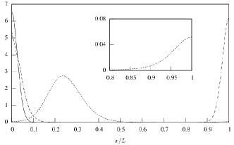
Figure 1: Fermion profiles for the parameter values described in Section V.3. Solid line = $Q_{L}$, short dash = $b_{R},\tau_{R}$, long dash = $t_{R},\nu_{R}$ and the dot-dash = $L_{L}$. Note that some of the fermions possess identical profiles. In particular the inset shows the identical profiles of $b_{R}$ and $\tau_{R}$ about $x/L=1$.

V.4 Simultaneously Suppressing Proton Decay and Obtaining Correct Fermion Masses

We have shown that our 5d QLLR setup enables us to obtain realistic fermion masses. However this setup does not allow one to suppress the proton decay rate. Proton decay occurs in the 5d QLLR model from operators of the form

$$O_{p}\sim\frac{1}{\Lambda^{9/2}}Q^{3}L\chi_{l}^{\dagger},$$ (92)

where $Q$ ($L$) denotes a quark (lepton) field and $\Lambda$ is the fundamental scale. As quarks and leptons have significant fifth dimensional wavefunction overlap with the setup in Section V.3 one must take the fundamental scale to be large or extend the model to ensure proton longevity. If one simply assumes the cutoff is large the usual fine tuning is required to stabilize the Higgs mass at the electroweak scale.

It was shown in Coulthurst:2006bc that models with a QLLR symmetry admit a split fermion setup which suppresses proton decay less arbitrarily than the split fermion implementation of the SM. This requires one of the localizing scalars to be odd (even) under Q $\leftrightarrow$ L ($1\leftrightarrow 2$). Unfortunately neither of the scalars in Section V.3 transformed in this way. If the fermion transformations of Eq. (87) are retained and one of the localizing scalars of Section V.3 is forced to be odd (even) under the Q $\leftrightarrow$ L ($1\leftrightarrow 2$) symmetry, the resulting fermionic geographies require large parameter hierarchies to produce realistic mass spectra. We instead choose $\Phi$ to be trivial under QL and the fermions to transform as

$$\begin{array}[]{ccccccc}L_{1}&\leftrightarrow&L_{2}&&L^{\prime}_{1}&\leftrightarrow&L^{\prime}_{2}\\ \updownarrow&{}\hfil&\updownarrow&&\updownarrow&{}\hfil&\updownarrow\\ Q_{1}&\leftrightarrow&Q^{\prime}_{2}&&Q^{\prime}_{1}&\leftrightarrow&Q_{2}\end{array}$$ (93)

under the QL and $1\leftrightarrow 2$ symmetries which leads to the mass relationship $m_{d}=m_{e}$. Choosing $\Sigma_{1}$ ($\Sigma_{2}$) to be odd (odd) under the $Q\leftrightarrow L$ symmetry and even (odd) under the $1\leftrightarrow 2$ symmetry, the localizing scalar Yukawa Lagrangian is

$$\mathcal{L_{\textrm{Yuk}_{\textrm{kink}}}} \sim f(\overline{Q_{1}^{c}}Q_{1}-\overline{L^{c}_{1}}L_{1}+\overline{Q_{2}^{\prime c}}Q_{2}^{\prime}-\overline{L^{c}_{2}}L_{2})\Sigma_{1}$$

$$+f^{\prime}(\overline{Q^{\prime c}_{1}}Q^{\prime}_{1}-\overline{L^{\prime c}_{1}}L^{\prime}_{1}+\overline{Q^{c}_{2}}Q_{2}-\overline{L^{\prime c}_{2}}L^{\prime}_{2})\Sigma_{1}$$

$$+g(-\overline{Q_{1}^{c}}Q_{1}+\overline{L^{c}_{1}}L_{1}+\overline{Q_{2}^{\prime c}}Q_{2}^{\prime}-\overline{L^{c}_{2}}L_{2})\Sigma_{2}$$

$$+g^{\prime}(-\overline{Q^{\prime c}_{1}}Q^{\prime}_{1}+\overline{L^{\prime c}_{1}}L^{\prime}_{1}+\overline{Q^{c}_{2}}Q_{2}-\overline{L^{\prime c}_{2}}L^{\prime}_{2})\Sigma_{2}.$$ (94)

If we take $f,f^{\prime},g,g^{\prime}>0$, all the right handed fermions are localized at the ends of the extra dimension, with quarks at one end and leptons at the other. Further, we find that $u_{R}$ ($d_{R}$) localized about $y=0$ has the same profile as $e_{R}$ ($\nu_{R}$) around $y=L$. Meanwhile the quark and lepton doublets have unrelated profiles with peaks in the bulk. This is precisely the setup advocated in Hung:2002qp ; Hung:2004ac to achieve a naturally small neutrino Dirac mass. That the leptons are lighter than the quarks now results from the lepton doublet been more strongly localised than the quark doublet. It then follows that we expect $m_{\nu}/m_{\tau}\ll m_{b}/m_{t}$ since the difference in the amplitudes of the right handed wave functions becomes more dramatic the further in to the bulk we move.

Again simplifying to the one generation case, the parameter choice $v_{1}=7.9/(\xi_{1}L),v_{2}=69/(\xi_{2}L)$ and $f=15.6\xi_{1},f^{\prime}=865\xi_{1},g=0.440\xi_{2},g^{\prime}=33.3\xi_{2}$, produces the fermion localization pattern shown in Figure 2. Note that the overlap between quarks and leptons is small enough to suppress the proton decay rate below current bounds with an order 10-100 TeV fundamental scale. If we take $\lambda_{t}=1.32$, $\lambda_{b}=\lambda_{\tau}=0.0713$ and $\lambda_{\nu}=0.3$, the fermion masses are $m_{t}=173\textrm{ GeV}$, $m_{b}=4.13\textrm{ GeV}$, $m_{\tau}=1.78\textrm{ GeV}$ and $m_{\nu}=77\textrm{ meV}$. This setup does contain some hierarchy: for $v_{1}\approx v_{2}$ one requires $\Lambda_{2}\approx 100\Lambda_{1}$ which leads to a hierarchy of $\mathcal{O}(10^{2})$ between the smallest and largest $\Sigma$ Yukawa coupling. This remains a vast improvement over the $\sim 12$ orders of magnitude parameter hierarchy required to explain fermion masses with Dirac neutrinos in the SM. It is also, to our knowledge, the first realization of the ideas of AS which implements both features of their proposal. Further work is required to check that this carries over to three generations and that, in particular, the SM mixing angles may be reproduced Twisting . However if this is shown to be the case this would represent the first dynamical setup to produce both realistic fermion masses and suppress proton decay via the split fermion mechanism.

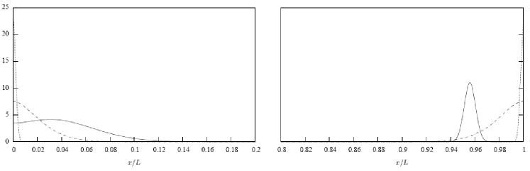
Figure 2: Fermion profiles for the parameter values described in Section V.4. Note only the regions around the ends of the extra dimension are plotted as all fermions have miniscule amplitudes in the central region. Quarks (leptons) are shown in the left (right) plot. Solid line=$Q_{L}(L_{L})$, short dash=$d_{R}(\nu_{R})$, dot-dash=$u_{R}(e_{R})$.

VI Neutral Currents

Having specified the fermion content we now present the neutral currents of the model and obtain bounds on the symmetry breaking scales $w_{R}$ and $w_{l}$. Since we consider $1/R\gg w_{l},w_{R}$ it shall suffice to consider the interactions of the zero mode fermions and gauge bosons. After changing to the neutral gauge boson mass eigenstate basis by diagonalizing the matrix $H$ with the rotation (109) the neutral current interactions for the zero mode fields may be written as

$${\cal L}_{NC}=\left[eA^{\mu}Q~{}+~{}\left(\frac{g}{\cos\theta}\right)~{}Z_{phy}^{\mu}~{}A_{NC}~{}+~{}\left(g\over\cos\theta\right)~{}Z_{phy}^{\prime\mu}~{}B_{NC}~{}+~{}\left(\frac{g}{\cos\theta}\right)~{}Z_{phy}^{\prime\prime\mu}~{}C_{NC}\right]~{}J_{NC,~{}\mu}^{00},$$ (95)

where the zero mode components of the current are

$$J^{00}_{NC,~{}\mu}=\sum_{i=1,2}\bar{Q}^{0}_{i}\gamma_{\mu}Q_{i}^{0}+\bar{Q}^{\prime 0}_{i}\gamma_{\mu}Q_{i}^{\prime 0}+\bar{L}^{0}_{i}\gamma_{\mu}L^{0}_{i}+\bar{L}^{\prime 0}_{i}\gamma_{\mu}L^{\prime 0}_{i},$$ (96)

and we have defined

$$A_{NC} = I_{3L}(U_{11}+\delta_{Z})-Q(U_{11}\sin^{2}\theta+\delta_{Z})+I_{3R}(U_{21}\cos\alpha\cos\theta+\delta_{Z})+T_{l}U_{31}\frac{g_{s}\cos\theta}{2g\cos\beta};$$ (97)

$$B_{NC} = I_{3L}(U_{12}+\delta_{Z^{\prime}})-Q(U_{12}\sin^{2}\theta+\delta_{Z^{\prime}})+I_{3R}(U_{22}\cos\alpha\cos\theta+\delta_{Z^{\prime}})+T_{l}U_{32}\frac{g_{s}\cos\theta}{2g\cos\beta};$$ (98)

$$C_{NC} = I_{3L}(U_{13}+\delta_{Z^{\prime\prime}})-Q(U_{13}\sin^{2}\theta+\delta_{Z^{\prime\prime}})+I_{3R}(U_{23}\cos\alpha\cos\theta+\delta_{Z^{\prime\prime}})+T_{l}U_{33}\frac{g_{s}\cos\theta}{2g\cos\beta},$$ (99)

where

$$\delta_{Z} = \sin\theta(U_{21}\tan\alpha+U_{31}\sec\alpha\tan\beta),$$ (100)

$$\delta_{Z^{\prime}} = \sin\theta(U_{22}\tan\alpha+U_{32}\sec\alpha\tan\beta),$$ (101)

$$\delta_{Z^{\prime\prime}} = \sin\theta(U_{23}\tan\alpha+U_{33}\sec\alpha\tan\beta),$$ (102)

where the form of the elements of $U$ may be found in Appendix A. These couplings may now be used to bound the symmetry breaking scales $w_{R,l}$. We achieve this by performing a $\chi^{2}$ fit of the predictions of this model to the following electroweak precision data:

$$R_{e,\mu,\tau,b,c}\quad,\quad A_{e,\mu,\tau,b,c,s}\quad,\quad A^{FB}_{e,\mu,\tau,b,c,s}\quad,$$

$$Q_{W}(Cs)\quad,\quad Q_{W}(Tl)\quad,\quad g_{n_{L}}^{2}\quad,\quad g_{n_{R}}^{2}\quad,$$

$$\Gamma_{Z}\quad,\quad\sigma_{\textrm{had}}\quad.$$ (103)

Under the phenomenological necessary assumption that $M_{Z^{\prime}}\gg M_{Z}$, the physical consequences of the corrections to the coupling of $Z_{phy}$ far outweigh the new physics resulting from the couplings to $Z^{\prime}_{phy}$. Thus we include only this dominant effect when determining our bounds. We find that in the LR limit one requires $w_{R}>4.8\textrm{ TeV}$ ($w_{R}>6.2\textrm{ TeV}$) at the 95% (90%) confidence level, which leads to $M_{Z^{\prime}}>2.7\textrm{ TeV}$ ($M_{Z^{\prime}}>3.4\textrm{ TeV}$). Note that we fit to more precision electroweak parameters than previous works using neutral currents to bound LR breaking scales and thus, to the best of our knowledge, this is the strongest bound on $w_{R}$ from the neutral sector yet obtained in the literature (for previous bounds see Czakon:1999ga ; Chay:1998hd ; Mimura:2002te ). In the QL limit, it is necessary that $w_{l}>1.5\textrm{ TeV}$ ($w_{l}>2.0\textrm{ TeV}$) and $M_{Z^{\prime}}>1.6\textrm{ TeV}$ ($M_{Z^{\prime}}>2.0\textrm{ TeV}$). If both $w_{R}$ and $w_{l}$ are close to their lower bounds, it is possible that $M_{Z^{\prime\prime}}$ is also at the TeV scale. In this case, at 95% confidence, we find $w_{R}>6.3\textrm{ TeV},w_{l}>2.1\textrm{ TeV}$ which leads to $M_{Z^{\prime}}>2.1\textrm{ TeV},M_{Z^{\prime\prime}}>3.5\textrm{ TeV}$. These bounds are shown in Figure 3.

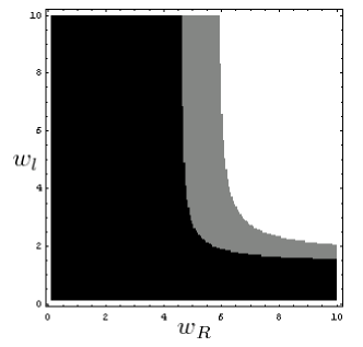
Figure 3: Plot of the values of $w_{R,l}$ which are consistent with a $\chi^{2}$ fit to the electroweak precision parameters (see equation (103) ). The grey (black) region is excluded at the 90% (95%) confidence level and the units are in TeV.

VII Experimental Signatures

In the limit $1/R\gg w_{l,R}$ the key signatures of 5d QLLR models result from the additional neutral gauge bosons and the liptons. The discovery of an additional neutral gauge boson at the LHC would be via Drell-Yann processes $pp\rightarrow Z^{\prime}\rightarrow l^{+}l^{-}$ Cvetic:1995zs ; Dittmar:2003ir . The lower center-of-mass energy of a next generation linear collider (NLC) precludes the production of real $Z^{\prime}$s. Thus any discovery at the NLC would be made by measuring $e^{+}e^{-}\rightarrow f\bar{f}$ and observing corrections resulting from interference between diagrams with a $Z^{\prime}$ propagator, and those with a $\gamma$ or $Z$ Cvetic:1995zs , to the relevant quantities discussed in Section VI.

Current data allows a $Z^{\prime}$ at TeV energies regardless of the hierarchy between $w_{l}$ and $w_{R}$, however the discovery prospects depend strongly on this hierarchy. In the limit $w_{R}<w_{l}$ the additional boson is basically that of the LR model. Previous studies have found that $Z^{\prime}_{LR}$ is discoverable up to a mass of about $5\textrm{ TeV}$ at the LHC (or NLC with $\sqrt{s}=1\textrm{ TeV}$) with an integrated luminosity of $100\mathrm{fb}^{-1}$ Cvetic:1995zs ; Rizzo:1996ce . If $w_{l}<w_{R}$ the light $Z^{\prime}$ is that of the QL model. In this case discovery at a hadron collider such as the LHC is unlikely since the cross section of the Drell-Yann process, $\sigma(pp\rightarrow Z^{\prime})B(Z^{\prime}\rightarrow l^{+}l^{-})$, will not be large. This is since $Z^{\prime}$ contains a large fraction of $G^{0}_{l}$ which does not couple to the quarks, meaning the cross section $\sigma(pp\rightarrow Z^{\prime})$ will be small. The discovery prospects are greater at the NLC since $G^{0}_{l}$ has large universal couplings to all leptons. These couplings are quite different from any of the canonical $Z^{\prime}$s usually considered, providing a distinctive signature.

The most interesting case is when $w_{R}\sim w_{l}$. Then both $Z^{\prime}$ and $Z^{\prime\prime}$ possess significant couplings to the $SU(3)_{l}$ and $SU(2)_{R}$ neutral currents and may have TeV masses. As such they could both be produced at the LHC. The prospects of discovery depend on the masses of the liptons, which are of order $w_{l}$. If the $Z^{\prime}$ bosons can decay into liptons their branching fraction into charged leptons will reduce and hence the Drell-Yann cross section will be smaller. The presence of light liptons would afford alternative discovery channels, with liptonic final states, at the LHC. At a linear collider light liptons are unimportant since only virtual $Z^{\prime}$s are produced. However, diagrams with both $Z^{\prime}$ and $Z^{\prime\prime}$ propagators will interfere with those of the SM, causing corrections. Without prior knowledge of the mass and mixings of the neutral gauge bosons their couplings to fermions are unknown. Thus separating their effects and categorically identifying the nature of the bosons is difficult.

If $w_{l}$ is at the TeV scale then the production of liptons is also possible at the LHC. For $1/R\gg w_{l}$, only the zero mode liptons with orbifold parity $(+,+)$, which are in different $SU(3)_{l}$ multiplets to the SM leptons, can be produced. Since both the $Y_{1,2}^{\pm}$ and $W_{R}$ bosons have $(+,-)$ orbifold parity, they do not directly couple the lightest liptons to the SM leptons. As the unbroken $SU(2)_{l}$ is expected to be confining these liptons will form bi-lipton bound states. These states will decay into SM fermions via creation of a $W$, $Z$ or photon. This will produce a clear experimental signature, the details of which are similar to those obtained in the 4d QLLR model Foot:1991fk .

VIII Conclusion

In this paper we have constructed and analysed the 5d QLLR model. We have shown that the higher dimensional construct permits a novel mechanism for suppressing neutrino masses below the electroweak scale and allows one to dramatically simplify the scalar sector employed in 4d constructs. This allows one to keep both the QL and the LR symmetry breaking scales low (TeV energies) so that two neutral gauge bosons may be observed at the LHC.

Split fermions were used to explain some of the features of the SM mass spectrum. Two interesting fermionic geographies were presented, each of which provided a rationale for the relationships $m_{t}>m_{b},m_{\tau}$ and $m_{\nu}\ll m_{t}$. One of these had no Yukawa coupling hierarchy but to suppress the proton decay rate required either a large cut-off or that the fundamental theory observed the accidental $B$ and $L$ symmetries of the QLLR model. In the former case, fine tuning was required to stabilize the Higgs boson mass at the electroweak scale. The alternative arrangement suppressed the proton decay rate by spatially separating quarks and leptons in the extra dimension. Thus the hierarchy problem was alleviated but at the cost of introducing an order $10^{2}$ Yukawa coupling hierarchy. Given the extent to which the symmetries of the model constrain the Yukawa sector it is a non-trivial result that interesting fermionic geographies can be obtained with mild Yukawa coupling hierarchies. These arrangements show promise but further work is required to ensure that a fully realistic three generational setup may be obtained.

Appendix A Neutral Gauge Boson Mixing

The physical $Z$-bosons are found by performing a 3-dimensional orthogonal rotation of the interaction $Z$-bosons. Defining

$$Z_{P} = (Z_{phy},Z_{phy}^{\prime},Z_{phy}^{\prime\prime})^{T},$$

$$Z_{I} = (Z,Z^{\prime},Z^{\prime\prime})^{T},$$ (104)

the relationship between the physical and interaction states is

$$Z_{P}=U^{-1}Z_{I},$$ (105)

with the diagonalized mass matrix being $D=U^{-1}HU$ and $H$ is defined in (43). We will parameterize the rotation matrix as

$$U(\zeta,\sigma,\psi)\equiv\left(\begin{array}[]{ccc}\cos\zeta\cos\psi-\cos\sigma\sin\zeta\sin\psi&\cos\psi\sin\zeta+\cos\zeta\cos\sigma\sin\psi&\sin\sigma\sin\psi\\ -\cos\sigma\cos\psi\sin\zeta-\cos\zeta\sin\psi&\cos\zeta\cos\sigma\cos\psi-\sin\zeta\sin\psi&\cos\psi\sin\sigma\\ \sin\zeta\sin\sigma&-\cos\zeta\sin\sigma&\cos\sigma\end{array}\right),$$ (109)

and we note that $U^{-1}(\zeta,\sigma,\psi)=U(-\psi,-\sigma,-\zeta)$. To order $\mathcal{O}\left(\frac{k^{4}}{w^{4}}\right)$ we find

$$U_{11}=1,$$ (110)

$$U_{21}=\frac{m_{Z}^{2}\cos^{3}\alpha\cos\theta(9w_{R}^{2}\sin^{4}\beta+4w_{l}^{2})}{2g^{2}w_{l}^{2}w_{R}^{2}},$$ (111)

$$U_{31}=\frac{-3\sqrt{3}m_{Z}^{2}\cos^{2}\alpha\cos\beta\cos\theta\sin^{2}\beta}{2gg_{s}w_{l}^{2}},$$ (112)

$$U_{33}=U_{22}=\sqrt{\mu_{+}}-m_{Z}^{2}\frac{g^{2}w_{R}^{2}}{4\Delta^{2}}\sin 2\theta\tan\beta\sqrt{\mu_{-}},$$ (113)

$$U_{23}=-U_{32}=\sqrt{\mu_{-}}+m_{Z}^{2}\frac{g^{2}w_{R}^{2}}{4\Delta^{2}}\sin 2\theta\tan\beta\sqrt{\mu_{+}},$$ (114)

$$U_{12} = -\left(\frac{m_{Z}^{2}}{M^{2}-\frac{1}{2}\Delta}\right)U_{33}\cos\alpha\cos\theta,$$ (115)

$$U_{13} = \left(\frac{m_{Z}^{2}}{M^{2}+\frac{1}{2}\Delta}\right)U_{32}\cos\alpha\cos\theta.$$ (116)

Expressing the mixing angles in terms of the elements $U_{ij}$ we have

$$\sigma = \arccos[U_{33}],$$ (117)

$$\zeta = \arcsin[U_{31}\csc\sigma],$$ (118)

$$\psi = \arcsin[U_{13}\csc\sigma],$$ (119)

if $\sigma\neq 0$ and

$$\psi+\zeta=-\arcsin U_{21},$$ (120)

if $\sigma=0$.

Appendix B Large LR Breaking Limit

In the limit $w_{R}\rightarrow\infty$ one has $U_{13}\rightarrow 0$ so that $\psi\rightarrow 0$. Thus

$$U=\left(\begin{array}[]{ccc}\cos\zeta&\sin\zeta&0\\ -\cos\sigma\sin\zeta&\cos\zeta\cos\sigma&\sin\sigma\\ \sin\zeta\sin\sigma&-\cos\zeta\sin\sigma&\cos\sigma\end{array}\right)$$ (124)

This may be written as $U=R_{\sigma}R_{\zeta}$ where

$$R_{\sigma}=\left(\begin{array}[]{ccc}1&0&0\\ 0&\cos\sigma&\sin\sigma\\ 0&-\sin\sigma&\cos\sigma\end{array}\right),$$ (128)

$$R_{\zeta}=\left(\begin{array}[]{ccc}\cos\zeta&\sin\zeta&0\\ -\sin\zeta&\cos\zeta&0\\ 0&0&1\end{array}\right),$$ (132)

so that

$$Z_{P} = U^{-1}Z_{I}$$ (133)

$$= R_{\zeta}^{-1}R_{\sigma}^{-1}Z_{I}$$

$$= R_{\zeta}^{-1}\tilde{Z}_{I},$$

where we have redefined the interaction basis as $\tilde{Z}_{I}=R_{\sigma}^{-1}Z_{I}$. In this basis, one of the additional neutral gauge bosons, $Z^{\prime\prime}_{QL}$, decouples in the large $w_{R}$ limit. The mixing between the SM $Z$ boson and the other additional neutral gauge boson, $Z^{\prime}_{QL}$, in this limit is given by $\zeta$. These extra gauge boson are

$$Z_{QL}^{\prime}=\cos\sigma Z^{\prime}-\sin\sigma Z^{\prime\prime},$$ (134)

$$Z_{QL}^{\prime\prime}=\sin\sigma Z^{\prime}+\cos\sigma Z^{\prime\prime},$$ (135)

with $Z^{\prime}$ and $Z^{\prime\prime}$ defined in (39) and the subscript emphasises that $Z_{QL}^{\prime}$ is the extra neutral boson found in the QL symmetric model.

References

- (1) For a review see R. N. Mohapatra, Unification and Supersymmetry, (Springer-Verlag, New York 1986).
- (2) R. Foot and H. Lew, Phys. Rev. D 41 (1990) 3502.
- (3) R. Foot and H. Lew, Nuovo Cim. A 104 (1991) 167.
- (4) R. Foot, H. Lew and R. R. Volkas, Phys. Rev. D 44, 1531 (1991).
- (5) N. Arkani-Hamed and M. Schmaltz, Phys. Rev. D 61, 033005 (2000) [arXiv:hep-ph/9903417].
- (6) Y. Mimura and S. Nandi, Phys. Lett. B 538, 406 (2002) [arXiv:hep-ph/0203126].
- (7) R. N. Mohapatra and A. Perez-Lorenzana, Phys. Rev. D 66, 035005 (2002) [arXiv:hep-ph/0205347].
- (8) G. Perez, Phys. Rev. D 67, 013009 (2003) [arXiv:hep-ph/0208102].
- (9) K. L. McDonald and B. H. J. McKellar, Phys. Rev. D 74, 056005 (2006) [arXiv:hep-ph/0609110].
- (10) A. Coulthurst, K. L. McDonald and B. H. J. McKellar, Phys. Rev. D 75, 045018 (2007) [arXiv:hep-ph/0611164].
- (11) A. Coulthurst, A. Demaria, K. L. McDonald and B. H. J. McKellar, arXiv:hep-ph/0611269.
- (12) R. Foot and R. R. Volkas, Phys. Lett. B 645, 345 (2007) [arXiv:hep-ph/0607047].
- (13) G. C. Joshi and R. R. Volkas, Phys. Rev. D 45, 1711 (1992).
- (14) K. S. Babu, E. Ma and S. Willenbrock, Phys. Rev. D 69, 051301 (2004) [arXiv:hep-ph/0307380].
- (15) S. L. Chen and E. Ma, Mod. Phys. Lett. A 19, 1267 (2004) [arXiv:hep-ph/0403105].
- (16) A. Demaria, C. I. Low and R. R. Volkas, Phys. Rev. D 72, 075007 (2005) [arXiv:hep-ph/0508160].
- (17) A. Demaria, C. I. Low and R. R. Volkas, Phys. Rev. D 74, 033005 (2006) [arXiv:hep-ph/0603152].
- (18) A. Demaria and K. L. McDonald, Phys. Rev. D 75, 056006 (2007) [arXiv:hep-ph/0610346].
- (19) There is a disagreement about the power of the term as Mohapatra:2002rn has a power of two. We have corresponded with the authors and they confirm a misprint.
- (20) M. Czakon, J. Gluza and M. Zralek, Phys. Lett. B 458, 355 (1999) [arXiv:hep-ph/9904216].
- (21) J. Chay, K. Y. Lee and S. H. Nam, Phys. Rev. D 61, 035002 (1999) [arXiv:hep-ph/9809298].
- (22) N. Arkani-Hamed, A. G. Cohen and H. Georgi, Phys. Lett. B 516, 395 (2001) [arXiv:hep-th/0103135].
- (23) Y. Grossman and G. Perez, Phys. Rev. D 67, 015011 (2003) [arXiv:hep-ph/0210053].
-
(24)
E. A. Mirabelli and M. Schmaltz, Phys. Rev D 61, 113011 (2000)
[arXiv:hep-ph/9912265];
D. E. Kaplan and T. M. P. Tait, JHEP 0111, 051 (2001) [arXiv:hep-ph/0110126];
G. Barenboim, G. C. Branco , A. de Gouvea and M. N. Rebelo, Phys. Rev. D 64, 073005 (2001) [arXiv:hep-ph/01040312];
B. Lillie, JHEP 0312, 030 (2003) [arXiv:hep-ph/0308091]. - (25) Such an approach may be taken consistently with the requirement for negligible Majorana neutrino masses. There are values for such that the Majorana masses will be sufficiently small to ignore but proton decay will proceed at rates above experimental bounds. Alternatively, the theory above the cut-off may preserve only , allowing proton decay to proceed but forbidding Majorana neutrino masses.
- (26) A. Coulthurst, K. L. McDonald and B. H. J. McKellar, Phys. Rev. D 74, 127701 (2006) [arXiv:hep-ph/0610345].
- (27) P. Q. Hung, Phys. Rev. D 67, 095011 (2003) [arXiv:hep-ph/0210131].
- (28) P. Q. Hung, Nucl. Phys. B 720, 89 (2005) [arXiv:hep-ph/0412262].
- (29) The masses must be run to a common scale which we take to be . This leads to running constants .
- (30) One complication when we begin considering a three generation model is that the fermion eigenstates which couple to need not coincide with the eigenstates coupling to . Most previous split fermion work, such as that listed in SFFlavour , has ignored this complication and assumed the coupling matrices are simultaneously diagonalizable. The implications when such ‘twisting’ is considered are discussed in Grossman:2004rm .
- (31) Y. Grossman, R. Harnik, G. Perez, M. D. Schwartz and Z. Surujon, Phys. Rev. D 71, 056007 (2005) [arXiv:hep-ph/0407260].
- (32) K. Chan and M. Cvetic, Phys. Lett. B375, 98 (1996) [arXiv:hep-th/9512188].
- (33) M. Dittmar, A. Nicollerat and A. Djouadi, Phys. Lett. B583, 111 (2004) [arXiv:hep-ph/0307020].
- (34) T. G. Rizzo, In the Proceedings of 1996 DPF / DPB Summer Study on New Directions for High-Energy Physics (Snowmass 96), Snowmass, Colorado, 25 Jun - 12 Jul 1996, pp NEW136 [arXiv:hep-ph/9612440].