GUCAS-CPS-07-03

hep-ph/0702271

Bell Inequalities in High Energy Physics

Abstract

We review in this paper the research status on testing the completeness of Quantum mechanics in High Energy Physics, especially on the Bell Inequalities. We briefly introduce the basic idea of Einstein, Podolsky, and Rosen paradox and the results obtained in photon experiments. In the tests of Bell inequalities in high energy physics, the early attempts of using spin correlations in particle decays and later on the mixing of neutral mesons used to form the quasi-spin entangled states are covered. The related experimental results in $K^{0}$ and $B^{0}$ systems are presented and discussed. We introduce the new scheme, which is based on the non-maximally entangled state and proposed to implement in $\phi$ factory, in testing the Local Hidden Variable Theory. And, we also discuss the possibility in generalizing it to the tau charm factory.

PACS number(s): 03.65.Fh, 14.40.Aq, 13.25.Gv

1 Introduction

Quantum Mechanics (QM) is one of the most important foundations of modern physics. However, the philosophic and physical debates on this fundamental theory are still continuing ever since its first presence. Among the various critiques on QM, the most important and famous one is what proposed by Einstein and his collaborators on whether the QM is a complete theory or not. Einstein, Podolsky, and Rosen (EPR) [1] questioned the completeness of QM by using a so-called Gedanken experiment which was then named the EPR paradox. In section 2 we introduce the EPR paradox in details, the explanation for the paradox in local hidden variable theory (LHVT), and the Bell theorem, which exhibits the contradiction of LHVT with QM and presents the non-locality nature of QM as the foundation of the modern quantum information theory. In section 3 we first introduce some optical experiments in testing the Bell inequalities. Then, we turn to the related studies in high energy physics in section 4. The last section is remained for conclusions for the past researches in testing the Bell Inequalities, and expectations for future investigations, especially in high energy physics.

2 From EPR to Bell inequalities

2.1 The EPR paradox

In 1935, Einstein, Podolsky, and Rosen demonstrated in a work [1] that quantum mechanics could not provide a complete description for the “physical reality” of two spatially separated but quantum mechanically correlated particle system. In the paper they described the following criterion of “physical reality”: if, without in any way disturbing a system, we can predict with certainty (i.e., with probability equal to unity) the value of a physical quantity, then there exists an element of physical reality corresponding to this physical quantity. Then they proposed the necessary condition for theories to be complete: every element of the physical reality must have a counterpart in the physical theory.

People noticed that the idealized experiment (Gedanken experiment) proposed by EPR is not suitable for designing the practical experiment. It requires to configure an entangled state, which is of the eigenstate of relative position and total momentum. However, this is not practical. Moreover, even if it could be constructed, such state cannot be a stationary state. It will only be in transitory existence, which makes the EPR argument fail.

Bohm [2] proposed a more realistic experiment which can illustrate the EPR paradox. He considered the two-particle spin-one-half system in spin singlet and zero angular momentum. in spin space, the wave function of this state can be expressed as

$$|\Psi\rangle=\frac{1}{\sqrt{2}}(|+\rangle_{A}|-\rangle_{B}-|-\rangle_{A}|+\rangle_{B})\;,$$ (1)

where the single particle states $|+\rangle$ and $|-\rangle$ denote “spin up” and “spin down” in certain coordinate frame. Assuming the two particle interaction does not involve spin-dependent term, particles are allowed to separate apart with the total spin of the system invariant, for example along the $y$ direction. When they are separated well beyond the range of interaction, we can measure the $z$-component of the spin of particle A. Due to angular moment conservation at all time, we can predict that the $z$-component of spin B must have the opposite value. In the meantime, because the spin singlet has spacial rotation invariance, the same thing happens when we measure the $x$-component of spin of particle A. Since the two particles are far apart with each other, the locality condition guarantees that the particle B does not know what happens to A while the measurement performs. Therefore, it shows that the B particle spins along $x$ and $z$ axes should be both physical realities. In QM the spin operators along different axes do not commute and thus can not simultaneously have definite values, therefore they can not be simultaneously in physical realities. Hence, Einstein concluded that QM must be incomplete.

Bohr contested not the EPR demonstration but their premises. His point of view is that an element of reality is associated with a concretely performed act of measurement. We can not perform the measurement along different axes simultaneously on particle A, so the spins of the particle B along different axes need not to be simultaneously physical realities. However, as Einstein questioned that these arguments make the reality of particle B depend upon the process of the measurement performed on the first particle, and he believed that “no reasonable definition of reality could be expected to do this.”

2.2 Bell inequalities

To avoid the EPR paradox, it might be a reasonable choice to postulate some additional ‘hidden variables’, which presumably will restore the completeness, determinism and causality to the theory. This kind of theories are named the local hidden variable theories. Nevertheless, once von Neumann, based on some axioms [3], demonstrated that it is impossible to construct such a hidden variable theory [4] reproducing all the results of QM. It was later on discovered that one of the von Neumann’s axioms in getting his conclusion is too much restrictive. And, indeed some counter examples were constructed in the two dimensional space [5]. That means the LHVT model can produce all the QM predictions but without fulfil von Neumann’s restrictive hypotheses. Nevertheless, there remains certain difference in between QM and LHVT. In 1964 Bell showed [6] that in realistic LHVTs the two particle correlation functions satisfy a set of Bell inequalities (BI), whereas the corresponding QM predictions may violate these inequalities in some region of parameter space. The definition of correlation for LHVTs and QM, according to Bohm, read respectively as:

$$E(\textbf{a},\textbf{b}) = \int\mathrm{d}\lambda\rho(\lambda)A(\textbf{a},\lambda)B(\textbf{b},\lambda)\;,$$ (2)

$$E(\textbf{a},\textbf{b}) = \langle\psi|\sigma\cdot\textbf{a}\otimes\sigma\cdot\textbf{b}|\psi\rangle=-\textbf{a}\cdot\textbf{b}\;.$$ (3)

Here, $\rho(\lambda)$ is the distribution of hidden variable regardless of whether $\lambda$ is a single variable or a set, or even a set of functions. These variables can be either discrete or continuous. a and b indicate spin directions. The original inequality obtained by Bell is

$$|E(\textbf{a},\textbf{b})-E(\textbf{a},\textbf{c})|-E(\textbf{b},\textbf{c})\leq 1\;,$$ (4)

where $\textbf{a},\textbf{b},\textbf{c}$ mean three different spin directions. In 1969, Clauser, Horne, Shimony, and Holt (CHSH) [7] generalized the inequality (4) to a more practical one, i.e.

$$S=|E(\textbf{a},\textbf{b})-E(\textbf{a},\textbf{b}^{\prime})|+E(\textbf{a}^{\prime},\textbf{b})+E(\textbf{a}^{\prime},\textbf{b}^{\prime})\leq 2\;.$$ (5)

A similar inequality to CHSH was derived by Bell in 1971 [8], read as

$$S=|E(\textbf{a},\textbf{b})-E(\textbf{a},\textbf{b}^{\prime})|+|E(\textbf{a}^{\prime},\textbf{b})+E(\textbf{a}^{\prime},\textbf{b}^{\prime})|\leq 2\;.$$ (6)

The correlation function $E$ in above inequalities is defined as

$$E(\textbf{a},\textbf{b})=P_{++}(\textbf{a},\textbf{b})-P_{+-}(\textbf{a},\textbf{b})-P_{-+}(\textbf{a},\textbf{b})+P_{--}(\textbf{a},\textbf{b})\;,$$ (7)

where $P_{\pm\pm}=N_{\pm\pm}(\textbf{a},\textbf{b})/N$, $N$ is the total number of particle pairs, and $N_{++(+-)}$ means that two particle has the same (opposite) spin directions. To suffice for experimental test, the total number of particle pair emissions $N$ should be known. However, in real practice the probability cannot be measured without either destroying or depolarizing the particle pairs. In 1974 Clauser and Horne (CH) [9] deduced an inequality, for which the upper limit is experimentally testable without knowing the $N$. That is

$$-1\leq P_{++}(\textbf{a},\textbf{b})-P_{++}(\textbf{a},\textbf{b}^{\prime})+P_{++}(\textbf{a}^{\prime},\textbf{b})+P_{++}(\textbf{a}^{\prime},\textbf{b}^{\prime})-P_{++}(\textbf{a}^{\prime},\infty)-P_{++}(\infty,\textbf{b})\leq 0,$$ (8)

where $P_{++}(\infty,\textbf{b})$ denotes the probability of finding a pair of particles with no polarization detection on one side. It is easy to find that the CH inequality (8) is consistent with inequality (6). Provided that in an experiment with two detectors and double channel analyzers, one can get three similar sets of inequalities like Eq.(8) with different indices $P_{-+},P_{+-},P_{--}$. Multiplying the inequalities with $P_{-+}$ and $P_{+-}$ by $-1$ and combining these four inequalities we can obtain the inequality (6).

It is generally realized that unlike the von Neumann’s mathematical results these inequalities can be reached in experiment in testing the validity of QM in comparison with LHVTs.

2.3 Generalizations of Bell theorem

Bell theorem reveals peculiar properties of quantum “entangled” states that were previously not appreciated. Many a generalization of Bell inequality aiming at getting optimal violations was developed. Better inequalities (inequalities with larger violation and/or wide range of parameter space for violation) are of both experimental and theoretical interest. In further development, one may create new inequalities, or explore the non-local character of a particular quantum state. Of course these two seemingly different investigation schemes are correlated.

Braunstein and Caves [10] made an extension of the inequality (6). They added two kinds of (6) up with different directions and got:

$$S=|E(\textbf{a},\textbf{b}^{\prime\prime})+E(\textbf{b}^{\prime\prime},\textbf{a}^{\prime\prime})+E(\textbf{a}^{\prime\prime},\textbf{b}^{\prime})+E(\textbf{b}^{\prime},\textbf{a}^{\prime})+E(\textbf{a}^{\prime},\textbf{b})-E(\textbf{b},\textbf{a})|\leq 4\;.$$ (9)

Usually, combining two inequalities directly will lead to an inequality with looser constraint than before. However Ref. [10] demonstrated that this kind of adding chain may lead to even stronger quantum violations. In this way, we may reexpress their result in a different form:

$$S_{N}=N|E(\pi/N)|\leq N-2\;,$$ (10)

where $N\geq 3$. It is very interesting to notice that when $N=3$ (10) corresponds to the maximal violation of (4); $N=4$ corresponds to the maximal violation of (6); and $N=6$ corresponds to the maximal violation of (9). Taking $\pi/N=\theta$, we have

$$|E(\theta)|\leq 1-\frac{2\theta}{\pi}\;,$$ (11)

which is similar to the Eq.(2.5) of [11]. Braunstein and Caves also put forward the idea of information-theoretic Bell inequalities [12]. The information-theoretic Bell inequalities was derived from the classical Shannon entropy and are violated by the quantum mechanical EPR pairs. This makes it possible to use the information theory to study the separability and nonlocality of quantum states. For more details, readers should refer to references [13, 14, 15, 16].

In 1989, Greenberger, Horne, and Zeilinger (GHZ) [17, 18] showed that for certain three and four particle entangled states there exists a conflict of QM prediction with local realism even for perfect correlation. That is the LHVT and QM can both make definite but opposite predictions. In 1992 Hardy proved [19], without using inequalities, this kind of definite confliction can occur for any non-maximally entangled state composed of two two-level subsystems. Later on Hardy’s argument was improved by Jordan [20]. He demonstrated that there exist four projection operators satisfying

$$\langle FG\rangle=0\;, \langle D(1-G)\rangle=0\;,$$ (12)

$$\langle(1-F)E\rangle=0\;, \ \ \ \langle DE\rangle>0\;,$$ (13)

which are in contradiction with LHVTs. In above and following equations, the alphabetic letter on the left side represents the projector of particle 1, and the right one for particle 2. Eq.(12) and Eq.(13) can be easily understood, i.e., if $D=1$ then $G=1$ according to the second equality of Eq.(12). And similarly if $E=1$ then $F=1$ according to the first equality of Eq.(13). From the second inequality of Eq.(13) we can infer that it is possible for $D$ and $E$ to be 1 simultaneously, and so are the $F$ and $G$. However, this is apparently in confliction with what the first equality of Eq.(12) tells. Jordan also demonstrated in a converse way [20] that for any choice of four different measurements, there exists a state satisfying Hardy’s argument. Garuccio in 1995 found [21] that the contradiction between QM and LHVT can be embedded in CH inequalities of (8), i.e.

$$\langle DE\rangle\leq\langle FG\rangle+\langle D(1-G)\rangle+\langle(1-F)E\rangle\;.$$ (14)

Along Hardy’s logic, Cabello [22] formulated a GHZ type of proof involving just two observers. Ref.[23] demonstrated that for the state that is a product of two singlet states, there exists a operator satisfying $F_{QM}=\langle\Psi|O|\Psi\rangle=9$ and $F_{LHVT}\leq 7$, which is obviously inconsistent. For recent developments on this respect one can find in the series works of Cabello’s [24, 25, 26].

Actually, the investigations on non-locality and the violation of Bell inequalities are not so transparent as explained above, especially when the mixed states and multi-particle high dimension systems are concerned. Since, it is not our main focus of this article, we suggest interested readers to refer to a recent review [27] and references therein.

3 Bell inequalities in optical experiment

Many experiments in regard of the Bell inequalities have been carried out by using the entangled photons. In the optical experiment the correlation of polarizers in orientations a and b is defined as follows:

$$E(\textbf{a},\textbf{b})=\frac{N_{++}(\textbf{a},\textbf{b})+N_{--}(\textbf{a},\textbf{b})-N_{+-}(\textbf{a},\textbf{b})-N_{-+}(\textbf{a},\textbf{b})}{N_{++}(\textbf{a},\textbf{b})+N_{+-}(\textbf{a},\textbf{b})+N_{-+}(\textbf{a},\textbf{b})+N_{--}(\textbf{a},\textbf{b})}\;,$$ (15)

where $N_{+-}$ is the coincidence rate of photon polarizations; $+$ for parallel and $-$ for perpendicular to the chosen direction. Of the various optical experiments, one of the important ones was carried out by Aspect et al. [28], in which the photons are generated from the atomic cascade radiation $J=0\rightarrow J=1\rightarrow J=0$. In the experiment they use the two-channel polarizers in orientations a and b, and a fourfold coincidence counting system by which the four coincidence rates $N_{\pm\pm}(\textbf{a},\textbf{b})$ can be measured in a single run, and they obtain directly the polarization correlation $E(\textbf{a},\textbf{b})$. Their measurement gave

$$S_{exp}=2.697\pm 0.015\;.$$ (16)

This result is in excellent agreement with the predictions of quantum mechanics, which, for their polarizer efficiencies and lens apertures, gives $S_{QM}=2.7\pm 0.05$. This experiment has been performed with the static setups in which polarizers are fixed for the whole duration of a run. A more important improvement of this experiment was made by the same group of people [29], in which they added two optical switches that can be randomly chosen in between two directions. The result also violates the upper limit of Bell’s inequality and in a good agreement with QM calculation.

Some other relevant and important progresses in this direction were realized by using the parametric down-conversion (PDC) [30, 31] technique in generating the entangled photon pairs. An ideal experiment with two channel polarizers, which randomly reoriented during the propagation of photons, has been fulfilled in real world [32]. The necessary space-like separation of the observation was achieved by keeping sufficiently large physical distance between the measurement stations (Alice and Bob was spatially 400m apart in the experiment), by ultra-fast and random setting of the analyzers, and by completely independent data registration. The experiment finally gave

$$S_{exp}=2.73\pm 0.02$$ (17)

for 14700 coincident events collected in 10s. This correspond to violation of the CHSH inequality of 30 standard deviations assuming only the statistical errors exist.

Recent measurements of the Bell inequality violation are realized through the multi-photon entangled states [33, 34]. It is directly applied to test the multi-photon generalizations of the Bell theorem [35]. The experimental result complies with the quantum mechanics prediction while contradicts with the LHVTs prediction by over 8 standard deviations [35].

The non-maximally entangled Hardy state was also realized in optical experiment [36]. The measurement further confirmed the QM but denied local realistic results [36]. A generalization [37] of Cabello’s argument in Ref.[23] was put into experiment in [38], using two photon four dimension entanglement (two polarization and two spatial degrees of freedom). The observable $F_{QM}=\langle\Psi|O|\Psi\rangle=8.56904\pm 0.00533$ gave a violation of LHVTs by about 294 standard deviations.

In all, for now all of the known experimental results [28, 29, 32, 35, 36, 38] in photon experiment are substantially consistent with the prediction of the standard QM. It is well-known that the main difficulty in the photon experiment is of the detect efficiency. Although the situation is improved in the PDC case, in practice the efficiency is still quite low. For example, the detection/collection efficiency is only abut 5% in [32]. As aforementioned the total number of emission is very important to the setup of correlation. To make these experimental measurements logically comparable to Bell inequalities one needs to make supplementary assumptions. That is: the ensemble of actually detected pairs is independent of the orientations of the polarimeters, and the detected photon pairs is a fair sample of the the ensemble of all emitted pairs. In the multi-photon case the similar detection loophole appears as well [27].

4 Bell inequalities in High Energy Physics

4.1 Motivations and some early attempts

People notice that the former experiments in testing the completeness of QM are mainly limited in the electromagnetic interaction regime, i.e., by employing the entangled photons, no matter whether the photons are generated from atomic cascade or PDC method. Considering of the fundamental importance of the concerned question, to test the LHVT in experiment with massive quanta and with other kinds of interactions is necessary [39].

To this aim, the spin singlet state, as first advocated by Bohm and Aharonov [2] to clarify the EPR argument, is exploited in experiment at the beginning. Lamehi-Rachti and Mitting [40] performed an experiment in the low energy proton-proton scattering at Saclay tandem accelerator. Their measurement of the spin correlation of protons gave a good agreement with what the QM tells.

As early as 1960s the EPR-like features of the $K^{0}\bar{K}^{0}$ pair in the decays of $J^{PC}=1^{--}$ vector particles were noticed by some authors [41, 42, 43, 44]. In the early attempts of testing LHVTs through the Bell inequality in high energy physics, people focused on exploiting the nature of particle spin correlations [39, 45, 46]. Typically, in Ref. [45] Törnqvist suggested to measure the BI through the following process:

$$e^{+}e^{-}\rightarrow\Lambda\bar{\Lambda}\rightarrow\pi^{-}\;p\;\pi^{+}\;\bar{p}\;.$$ (18)

Two different decay modes of $\eta_{c}\rightarrow\Lambda\bar{\Lambda}$ and $J/\psi\rightarrow\Lambda\bar{\Lambda}$ are considered by Törquist. In Ref.[11] the matrix element for $\eta_{c}$ or $J/\psi$ decay generically takes the following form:

$$A\propto\sum_{ij}\langle\chi_{p}|\textbf{M}_{a}|\chi_{\Lambda_{i}}\rangle s_{i\!j}\langle\chi^{\dagger}_{\bar{\Lambda}_{j}}|\textbf{M}^{\dagger}_{b}|\chi^{\dagger}_{\bar{p}}\rangle\;.$$ (19)

Here, $M_{i}$ represents the interaction which induces the hadronic transition of $\Lambda$ to final states. $s_{ij}$ represents spin structure of the charmonium. After taking the standard procedure, one obtain the transition probability. For example, for $\eta_{c}$ decay it reads:

$$R(\hat{\textbf{a}},\hat{\textbf{b}})\propto 1+\alpha^{2}\hat{\textbf{a}}\cdot\hat{\textbf{b}}\;,$$ (20)

where $\alpha$ denotes the $\Lambda$ decay asymmetry parameter; $\hat{\textbf{a}}$ and $\hat{\textbf{b}}$ are unit vectors along the $\pi^{+}$ and $\pi^{-}$ momenta in $\bar{\Lambda}$ and $\Lambda$ rest frame, respectively. Törnqvist argued that apart from the constant $\alpha^{2}$ and the sign before $\hat{\textbf{a}}\cdot\hat{\textbf{b}}$, (20) is in equivalence with Eq.(3) obtained in measuring the spin correlation in the Bohm’s Gedanken experiment. Here, the directions of the pion momentum $\hat{\textbf{a}}$ and $\hat{\textbf{b}}$ take the place of the spin-analyzing directions of the polarimeters.

For $J/\psi$ decays,

$$R(\hat{\textbf{a}},\hat{\textbf{b}})\propto 2(1-\frac{k^{2}}{E^{2}_{\Lambda}}\sin^{2}\theta)(1-\alpha^{2}\hat{a}_{n}\hat{b}_{n})+\frac{k^{2}}{E^{2}_{\Lambda}}\sin^{2}\theta[1-\alpha^{2}(\hat{\textbf{a}}\cdot\hat{\textbf{b}}-2\hat{a}_{x}\hat{b}_{x})]\;.$$ (21)

The DM2 Collaboration [47] observed $7.7\times 10^{6}\ J/\psi$ events with about $10^{3}$ being identified as from process $J/\psi\rightarrow\Lambda\bar{\Lambda}\rightarrow\pi^{-}p\pi^{+}\bar{p}$. The experimental measurement unfortunately does not give a very significant result[11] due to the insufficient statistics.

A similar process was suggested by Privitera [46], i.e.,

$$e^{+}e^{-}\rightarrow\tau^{+}\tau^{-}\rightarrow\pi^{+}\bar{\nu}_{\tau}\pi^{-}\nu_{\tau}\;.$$ (22)

In analogy with what in charmonium decays, in this case the expected correlation rate is given by

$$N(\hat{\textbf{p}_{1}},\hat{\textbf{p}_{2}})\propto 1-\frac{1}{3}\hat{\textbf{p}_{1}}\cdot\hat{\textbf{p}_{2}}\;,$$ (23)

where $\hat{\textbf{p}}_{1}$ and $\hat{\textbf{p}}_{2}$ are unit vectors in the momentum directions of $\pi^{+}$ and $\pi^{-}$, respectively. Hereby, the strong spin correlation between two $\tau$’s reveals the nonlocal nature of the EPR argument. The subsequent $\tau$ decay works as a spin analyzer, and the correlation is transferred to the decay products.

The above mentioned designs for experimentally measuring the violation of BI are delicate and attractive, however, people found that such proposals possess controversial assumptions [48]. They all assume that the decay matrix elements contain the nonlocal correlations, i.e., Eq.(20, 21, 23). However, there is no dichotomic observable which can be directly measured in real experiment. The momentum of pion is a continuous variable, and different momenta are compatible, i.e. [$(\hat{P}_{\pi^{+}})_{i}$, $(\hat{P}_{\pi^{-}})_{j}$] = 0 [39, 48]. Thus a LHVT can be constructed in respect of all the results from QM, and there will be no violation of Bell inequality anyway.

4.2 Testing correlation by virtue of quasi-spin

In testing the LHVTs in high energy physics, using the “quasi-spin” to mimic the photon polarization in the construction of entangled states is a practical way. For example, for kaon the quantum number of strangeness $S$, which takes either 1 or -1, can play the role of spin. Several groups suggested to study the $K^{0}\bar{K}^{0}$ system in the $\phi$ factory to test the LHVT (for details, see Ref. [49] and references therein). Up to now, there are two different ways in the “quasi-spin” scheme. In the first way, one fixes up the quasi-spin, but leaves the freedom in time. For example, one measures the Flavor Taste in different decaying time on each side, then the time differences plays the role of polarization angles. The second one is to leave the freedom in quasi-spin but to fix the time. In this case we measure the different eigenstates of the particles at the same time on each side, then the different eigenstates play the role of polarization angles.

A typical process produces entangled state in $K^{0}\bar{K}^{0}$ system is through $e^{+}e^{-}\rightarrow\phi\rightarrow K^{0}\bar{K}^{0}$. The wave function of the $J^{PC}=1^{--}$ particles, like $\phi$ which decays into $K^{0}\bar{K}^{0}$, can be formally configured as [50]:

$$|\phi\rangle=\frac{1}{\sqrt{2}}\{|K^{0}\rangle|\bar{K}^{0}\rangle-|\bar{K}^{0}\rangle|K^{0}\rangle\}\;.$$ (24)

Similar expressiones apply to $\Upsilon(4S)\rightarrow B^{0}\bar{B}^{0}$, $\Upsilon(5S)\rightarrow B_{s}^{0}\bar{B}_{s}^{0}$, and $\psi(3770)\rightarrow D^{0}\bar{D}^{0}$ cases.

In the following we explain the above mentioned techniques in a bit details. First, we consider the situation in which the meson state takes place of spin polarization discussed in preceding sections. For kaon system, there are three different kinds of eigenstates, those are: the mass, $CP$, and Strangeness.

We define the effect of $\hat{C}\hat{P}$ operators acting on the $K^{0}$ and $\bar{K}^{0}$ states, like

$$\hat{C}\hat{P}|K^{0}\rangle = |\bar{K}^{0}\rangle\;,$$ (25)

$$\hat{C}\hat{P}|\bar{K}^{0}\rangle = |K^{0}\rangle\;,$$ (26)

up to an arbitrary phase. With this choice in phase the $CP$ eigenstates can be expressed as:

$$|K^{0}_{1}\rangle = \frac{1}{\sqrt{2}}\{|K^{0}\rangle+|\bar{K}^{0}\rangle\}\;,$$ (27)

$$|K^{0}_{2}\rangle = \frac{1}{\sqrt{2}}\{|K^{0}\rangle-|\bar{K}^{0}\rangle\}\;.$$ (28)

And correspondingly the mass eigenstates are:

$$|K_{S}\rangle = \frac{1}{N}\{p|K^{0}\rangle+q|\bar{K}^{0}\rangle\}\;,$$ (29)

$$|K_{L}\rangle = \frac{1}{N}\{p|K^{0}\rangle-q|\bar{K}^{0}\rangle\}\;,$$ (30)

where $p=1+\varepsilon,q=1-\varepsilon$, and $N^{2}=|p|^{2}+|q|^{2}$. The $\varepsilon$ is the normal $CP$ violation parameter. With above knowledge, Eq.(24) can be reexpressed as:

$$|\phi\rangle = \frac{1}{\sqrt{2}}\{|K_{2}\rangle|K_{1}\rangle-|K_{1}\rangle|K_{2}\rangle\}\;,$$ (31)

$$|\phi\rangle = \frac{N^{2}}{2\sqrt{2}pq}\{|K_{L}\rangle|K_{S}\rangle-|K_{S}\rangle|K_{L}\rangle\}\;.$$ (32)

It is more convenient to use Wigner’s inequality which can be derived from Eq. (4) [49], i.e.:

$$P(\textbf{a},\textbf{b})\leq P(\textbf{a},\textbf{c})+P(\textbf{b},\textbf{c})\;,$$ (33)

where $\textbf{a},\textbf{b},\textbf{c}$ are the same as in Eq.(4) and $P$s represent the probabilities with subscripts in (8) suppressed. According to Ref. [51], we chose the following states as the quasi-spin:

a $$= |K_{S}\rangle\;,$$ (34)

b $$= |K^{0}\rangle\;,$$ (35)

c $$= |K_{1}\rangle\;.$$ (36)

Then, the inequality (33) turns to be

$$P(m_{S},S=+1)\leq P(m_{S},CP+)+P(CP+,S=+1)\;,$$ (37)

where $P(m_{S},S=+1)$ means the coincident rate while on one side it is found to be $K_{S}$ and on the other side is found to be $K^{0}$. The same notation applies to $P(m_{S},CP+)$ and $P(CP+,S=+1)$. Substitute (28) and (30) into (37), the inequality becomes [51]:

$$\rm{Re}\{\varepsilon\}\leq|\,\varepsilon|^{2},$$ (38)

which is obviously violated by the experimental measurements on $\varepsilon$ [52]. It is interesting to notice that as b taken to be $|\bar{K}^{0}\rangle$, (33) becomes $-\rm{Re}\{\varepsilon\}\leq|\,\varepsilon|^{2}$ [53], and it will be always true. As pointed out in Ref.[49], the (38) is taken at the beginning time, when the entangled kaon pairs are not well separated; what tested is only the contextuality rather than non-locality.

As mentioned in above, we can also choose different time to measure the final states, the kaons, on each side. For illustration, we choose the quantum number of Strangeness as the quasi-spin in our consideration, but neglect the CP violation effect, which in some sense is a good approximation.

With the time evolution, the initial entangled state, like in (24), becomes:

$$|\Psi(t_{l},t_{r})\rangle=\frac{1}{\sqrt{2}}\{e^{-i(m_{L}t_{l}+m_{S}t_{r})}e^{-\frac{\Gamma_{L}}{2}t_{l}-\frac{\Gamma_{S}}{2}t_{r}}|K_{L}\rangle|K_{S}\rangle$$

$$-e^{-i(m_{S}t_{l}+m_{L}t_{r})}e^{-\frac{\Gamma_{S}}{2}t_{l}-\frac{\Gamma_{L}}{2}t_{r}}|K_{S}\rangle|K_{L}\rangle\}\;.$$ (39)

Here in above, the small letters $l$ and $r$ denote left side and right side, suppose we name the two entangled particles to be left and right without lose generality. Chooseing different measurement time for two sides, we have the coincident rate [54]:

$$P(K^{0},t_{l};K^{0},t_{r}) = P(\bar{K}^{0},t_{l};\bar{K}^{0},t_{r})$$ (40)

$$= \frac{1}{8}\{e^{-\Gamma_{L}t_{l}-\Gamma_{S}t_{r}}+e^{-\Gamma_{S}t_{l}-\Gamma_{L}t_{r}}-2e^{-\frac{\Gamma_{L}+\Gamma_{S}}{2}(t_{l}+t_{r})}\cos(\Delta m\Delta t)\}\;,$$

$$P(K^{0},t_{l};\bar{K}^{0},t_{r}) = P(\bar{K}^{0},t_{l};K^{0},t_{r})$$ (41)

$$= \frac{1}{8}\{e^{-\Gamma_{L}t_{l}-\Gamma_{S}t_{r}}+e^{-\Gamma_{S}t_{l}-\Gamma_{L}t_{r}}+2e^{-\frac{\Gamma_{L}+\Gamma_{S}}{2}(t_{l}+t_{r})}\cos(\Delta m\Delta t)\}\;.$$

Here, $P(K^{0}(\bar{K}^{0}),t_{l};K^{0}(\bar{K}^{0}),t_{r})$ represents the probability of finding $K^{0}(\bar{K}^{0})$ on the left side at time $t_{l}$ and $K^{0}(\bar{K}^{0})$ on the right side at time $t_{r}$. The expectation value of correlation is:

$$E(t_{l},t_{r})=-\cos(\Delta m\Delta t)e^{-\frac{\Gamma_{L}+\Gamma_{S}}{2}(t_{l}+t_{s})}\;.$$ (42)

Inserting this correlation directly to CHSH inequality, one can immediately find that the violation of inequality depend on the ratio of $x=\Delta m/\Gamma$ [49], where the $\Delta m$ characterizes of Strangeness oscillation and the $\Gamma$ characterizes the weak decays. For the case of $x$ being small, that means the oscillation is dominated by the weak decays, there will be no violation of CHSH inequalities. Among the known neutral mesons, only $B^{0}_{S}\bar{B}^{0}_{S}$ system has a big enough experimental value of $x$, and hence the violation of inequalities might be found there [49].

The EPR-type Strangeness correlation in the process $p\bar{p}\rightarrow K^{0}\bar{K}^{0}$ has been tested at the CPLEAR detector [55] at CERN. In the experiment the $K^{0}\bar{K}^{0}$ pairs were created in $J^{PC}=1^{--}$ configuration. The wave function at proper time $t_{l}=t_{r}=0$ is

$$|\Psi(0,0)\rangle=\frac{1}{\sqrt{2}}[|K^{0}\rangle_{l}|\bar{K}^{0}\rangle_{r}-|\bar{K}^{0}\rangle_{l}|K^{0}\rangle_{r}]\;.$$ (43)

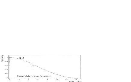
Figure 1: The best fit to the experimental measurement [55]. The two points with error bars correspond to time difference $\Delta t=0$ and $\Delta t=1.2\tau_{s}$. The solid line represents the QM prediction.

In the experiment, two kinds of measurements were performed. The first one was to perform the measurements on each side of the source at the same time. Another one was to perform the measurements in different distances (so was the time) for the two sides. The strangeness was tagged via strong interaction with absorbers away from the creation point. The measured Strangeness asymmetry is

$$A(t_{l},t_{r})=\frac{I_{unlike}(t_{l},t_{r})-I_{like}(t_{l},t_{r})}{I_{unlike}(t_{l},t_{r})+I_{like}(t_{l},t_{r})}\;.$$ (44)

Here, $I_{(un)like}$ means the (un)like strangeness event, which are defined as

$$I_{like}(t_{l},t_{r}) = P(K^{0},t_{l};K^{0},t_{r})+P(\bar{K}^{0},t_{l};\bar{K}^{0},t_{r})\;,$$ (45)

$$I_{unlike}(t_{l},t_{r}) = P(K^{0},t_{l};\bar{K}^{0},t_{r})+P(\bar{K}^{0},t_{l};K^{0},t_{r})\;.$$ (46)

From Fig.1 one notices that the non-separability hypothesis of QM is strongly favoured by experiment.

The $B^{0}\bar{B^{0}}$ entangled system produced at the $\Upsilon(4S)$ resonance has also been measured in the B-factory [56]. The wave function of $\Upsilon(4S)\rightarrow B^{0}\bar{B^{0}}$ has the same formalism as the spin singlet:

$$|\Upsilon\rangle=\frac{1}{\sqrt{2}}\{|B^{0}\rangle_{l}|\bar{B^{0}}\rangle_{r}-|\bar{B^{0}}\rangle_{l}|B^{0}\rangle_{r}\}\;.$$ (47)

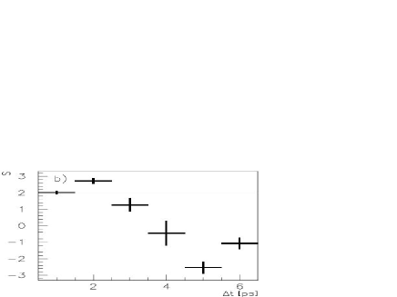
Figure 2: The experiment result of the violation of inequality [56]. The horizontal axis refers to $\Delta t$ and the vertical axis to the S. The LHVTs limit of 2 is shown by the solid line.

Here, the quantum number of flavor plays the role of spin polarization in the spin correlation system. In the first method, i.e. with fixed quasi-spin and free in time, the correlation function for $B^{0}\bar{B^{0}}$ system reads

$$E(t_{l},t_{r})=-e^{-\frac{2t^{\prime}+\Delta t}{\tau_{B}}}\cos(\Delta m_{d}\Delta t)\;,$$ (48)

where $\Delta m_{d}$ characterizes the $B^{0}-\bar{B^{0}}$ mixing, $\tau_{B}$ is the $B^{0}$ decay mean time, $t^{\prime}=\min(t_{l},t_{r})$, and $\Delta t=|t_{l}-t_{r}|$. Normalizing the above correlation function by the undecayed $B^{0}$ pairs, one then gets the correlation function as

$$E_{R}(\Delta t)=-\cos(\Delta m_{d}\Delta t)\;.$$ (49)

Put it into the Bell-CHSH inequality, one can get the violation parameter [56]

$$S(\Delta t)=3E_{R}(\Delta t)-E_{R}(3\Delta t)\leq 2\;.$$ (50)

The experiment, which based on the data sample of $80\times 10^{6}$ $\Upsilon(4S)\rightarrow B\bar{B}$ decays at Belle detector at the KEKB asymmetric collider in Japan, tells $S=2.725\pm 0.167_{stat}$. It is obviously a result violating the Bell inequality, as shown in Fig.2.

In spite of the achievements in the high energy physics experiments mentioned in above, theoretically, debate on whether the quasi-spin of unstable particle can give a genuine test of LHVTs or not remains [57]. If the neutral mesons are stable, the analogy of quasi-spin with spin would be perfect. However, in reality the unstable particles may decay, and hence, in principle on should include the Hilbert space of all decay products as well [49]. By the unitary time evolution of the unstable state, some information may lose into the decay products. In addition, there is another major difference between real- and quasi-spin systems. For the former, one can detect arbitrarily the spin state $\alpha|+\rangle+\beta|-\rangle$; however, it is not true in the quasi-spin, the mesons pairs, system. This difference may induce problem for the neutral meson systems. That is, the passive measurement nature of quasi-spin meson system makes the possibility to choose freely the quasi-spin among alternative setups lost. In CPLEAR experiment the active measurement requirement is fulfilled, because the neutral kaon meson is identified through strong interaction with the absorber. While in the B meson case, there is no way for experimenter to force B-meson to decay at a given instant $t_{l}$ or $t_{l^{\prime}}$ [57]. As of the unitary condition, the Eq.(49) for B-meson system is different from Eq.(42). For B-meson system, it is normalized by the undecayed $B^{0}\bar{B^{0}}$ pairs, which, like in the photon case, asks some additional assumptions to make the correlation to be comparable to what required by the Bell inequality because of the detecting efficiency.

Recently, the $B_{S}^{0}\bar{B}^{0}_{S}$ pair production is observed in experiment in $\Upsilon(5S)$ decays [58, 59]. $B^{0}_{S}$ meson has a suitable $x$ value for the violation of CHSH inequality, even if the interplay of weak interaction is considered, we expect that measurement on $B_{S}^{0}\bar{B}^{0}_{S}$ mixing in the future may give another notable test of the QM correlation.

4.3 Some Novel Ideas in Testing LHVT in High Energy Physics

Recently, based on the Hardy’s approach Bramon and Garbarino propose a new scheme [60, 61] to test the local realism by virtue of entangled neutral kaons. After neglecting the small CP-violation effect, the initial $K_{S}K_{L}$ pair from $\phi$ decay, or proton-antiproton annihilation, is the same as (32), i.e.

$$|\phi(T=0)\rangle=\frac{1}{\sqrt{2}}[K_{S}K_{L}-K_{L}K_{S}]\ ,$$ (51)

where $K_{S}=(K^{0}+\bar{K^{0}})/\sqrt{2}$ and $K_{L}=(K^{0}-\bar{K^{0}})/\sqrt{2}$ are the mass eigenstates of the $K$ mesons. One of the key points in using kaon system to test the LHVTs is to generate a nonmaximally entangled (asymmetric) state. That is

$$|\phi(T)\rangle=\frac{1}{\sqrt{2+|R|^{\,2}}}\,[K_{S}K_{L}-K_{L}K_{S}-re^{-i(m_{L}-m_{S})\,T+[(\Gamma_{S}-\Gamma_{L})/2]T}K_{L}K_{L}]\ .$$ (52)

Here, $r$ is the regeneration parameter to be the order of magnitude $10^{-3}$ [61]; $\Gamma_{L}$ and $\Gamma_{S}$ are the $K_{L}$ and $K_{S}$ decay widths, respectively; T is the evolution time of kaons after their production. Technically, this asymmetric state can be achieved by placing a thin regenerator close to the $\phi$ decay point [60].

Four specific transition probabilities for joint measurements from QM take the following forms:

$$P_{QM}(K^{0},\bar{K^{0}}) \equiv |\langle K^{0}\bar{K^{0}}|\phi(T)\rangle|^{\ 2}$$ (53)

$$= \frac{|2+\mathrm{R}e^{i\varphi}|^{\,2}}{4(2+|R|^{2})}\ ,$$

$$P_{QM}(K^{0},K_{L}) \equiv |\langle K^{0}K_{L}|\phi(T)\rangle|^{\ 2}$$ (54)

$$= \frac{|1+\mathrm{R}e^{i\varphi}|^{\,2}}{2(2+|R|^{2})}\ ,$$

$$P_{QM}(K_{L},\bar{K^{0}}) \equiv |\langle K_{L}\bar{K_{0}}|\phi(T)\rangle|^{\ 2}$$ (55)

$$= \frac{|1+\mathrm{R}e^{i\varphi}|^{\,2}}{2(2+|R|^{2})}\ ,$$

$$P_{QM}(K_{S}K_{S}) \equiv |\langle K_{S}K_{S}|\phi(T)\rangle|^{\ 2}=0\ ,$$ (56)

where $\mathrm{R}=-|R|=-|r|e^{[(\Gamma_{S}-\Gamma_{L})/2]T}$ and $\varphi$ is the phase of $R$. In Ref. [61] the special case of $R=-1$ was considered, in which

$$P_{QM}(K^{0},\bar{K^{0}}) = 1/12\;,$$ (57)

$$P_{QM}(K^{0},K_{L}) = 0\;,$$ (58)

$$P_{QM}(K_{L},\bar{K^{0}}) = 0\;,$$ (59)

$$P_{QM}(K_{S},K_{S}) = 0\;.$$ (60)

From (13) and in light of the arguments in Ref. [61], in the following we demonstrate how LHVTs conflict with QM in this case.

Suppose in a typical experiment, the strangeness on both sides at a proper time T is measured. For example, a detection of $K^{0}$ on the left side and $\bar{K^{0}}$ on the right side is achieved. We know this may happen from Eq.(57), and then we can infer from (58) that if the decay on the right hand side is observed, the $K_{S}$ exits there for certain. In this case, according to Einstein’s argument the $K_{S}$ on the right side corresponds to a physical reality. Similarly, if we have measured the lifetime of kaon on the left side, according to (59) one can confirm that it should be $K_{S}$. In all, the non-zero probability of $P_{QM}(K^{0},\bar{K^{0}})$ leads to the non-zero probability of $K_{S}$ on both sides. However, due to EPR’s criterion of “physical reality” this is in contradiction with Eq.(60). This kind of contradiction need a null measurement of the transition probability of Eq.(60) that cannot be strictly performed. Starting from (14) Bramon et al. derived out the following Eberhard’s inequality (EI) [62], i.e.,

$$H_{LR}\equiv\frac{P_{LR}(K^{0},\bar{K^{0}})}{P_{LR}(K^{0},K_{L})+P_{LR}(K_{S},K_{S})+P_{LR}(K_{L},\bar{K^{0}})+P(K^{0},U_{Lif})+P(U_{Lif},\bar{K^{0}})}\leq 1,$$ (61)

where $P_{\rm{LR}}$ denotes the transition probability in LHVTs with the subscripts LR symbolizing the local realism. $H_{LR}$ means the local realistic value of the fraction which must less than 1 according to LHVTs. $U_{Lif}$ denotes the failures in lifetime detection. In Ref.[62] the above inequality is used in deducing the possible violation, which depends upon the restriction of experimental efficiencies. Unlike the null measurement this inequality can tolerate with the unsatisfied experimental efficiencies.

For simplicity we consider an ideal case, in which the detection efficiency of the kaon decays is 100 percent. Then the EI for the kaon system takes the similar form as Eq.(14) [63, 21]. It reads

$$P_{LR}(K^{0},\bar{K^{0}}) \leq P_{LR}(K^{0},K_{L})+P_{LR}(K_{S},K_{S})+P_{LR}(K_{L},\bar{K^{0}})\ .$$ (62)

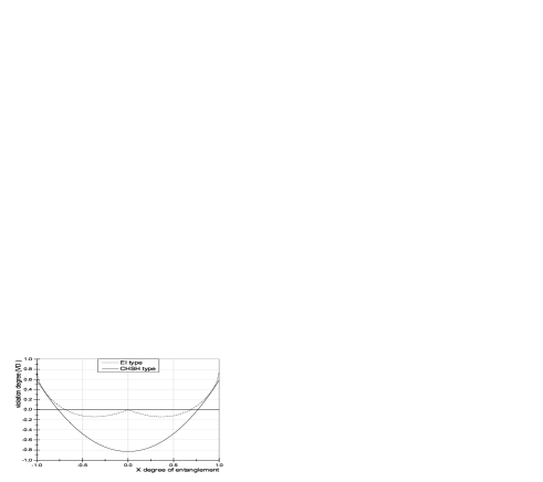
Figure 3: The violation degree of the Bell inequalities (the dashed line for EI type and the solid line for CHSH type) in terms of the entanglement. Here, for the sake of transparency, we make a coordinator exchange, the $C=1-x^{2}$. The magnitudes of $V\!\!D$ less than zero means the broken of the BIs.

For the case of QM, substituting equations (53) - (56) into the inequality (62) and assuming $\varphi=0$, we have

$$\frac{(2+\mathrm{R})^{2}}{4(2+\mathrm{R}^{2})} \leq \frac{(1+\mathrm{R})^{2}}{2(2+\mathrm{R}^{2})}\;+\;0\;+\;\frac{(1+\mathrm{R})^{2}}{2(2+\mathrm{R}^{2})}\ .$$ (63)

The above inequality is apparently violated by QM while $\mathrm{R}=-1$. In Ref. [64] we generalized the method used in [61] to heavy quarkonium. This straightforward generalization however leads to some new observations of the nonlocal property. Upon further analyzing the R value when it gives violation of Eq.(63), we find out that there exist a period of time during which the violation became larger through time evolution. In quantum information theory the entanglement property of two qubits pure state are well understood, which can be characterized by the concurrence $C$ [65]. We can also see how the degree of entanglement evolves with time. Here, according to the definition of concurrence we have

$$C(J/\psi)=|\langle J/\psi|\widetilde{J/\psi}\rangle|=\frac{2}{2+|R|^{\,2}}=\frac{2}{2+|r|^{\,2}e^{(\Gamma_{S}-\Gamma_{L})\,T}}\ ,$$ (64)

where $|\widetilde{J/\psi}\rangle=\sigma^{1}_{y}\sigma^{2}_{y}|(J/\psi)^{*}\rangle\$ and $\sigma^{1,\ 2}$ are Pauli matrices. $C$ changes between null to unit for no entanglement and full entanglement. Eq.(64) shows that the state become less entangled with the time evolution. So, considering of (63) we realize that the violation of it does not decrease monotonously with the degree of entanglement. To clarify this phenomenon we express the violation degree ($V\!\!D$) of the inequalities (left side minus the right side) in term of $C$ and compare it with the usual CHSH inequality [7]. In Figure 3 different $V\!\!D$ behaviors of CHSH’s and Eberhard’s inequalities are presented. For CHSH case, the $V\!\!D_{\rm CHSH}$ is obtained in the same condition as the maximal violation happens in the full entanglement, the $C=1$. We have:

$$V\!\!D_{CHSH}=\sqrt{2}(1+C)-2\ .$$ (65)

In fact, the above $V\!\!D_{\rm CHSH}$ can be deduced from the results given in Refs. [66, 67, 68]. For EI case,

$$V\!\!D_{EI}=\frac{-3(1-C)+2\sqrt{2}\sqrt{C-C^{2}}}{4}\ .$$ (66)

Here, in EI the counterintuitive quantum effect shows up, i.e. the less entanglement corresponding to a larger $V\!\!D$ in some region (see Fig.3). It is worthy to notice that with the time evolution, when $R$ becomes less than $-\frac{4}{3}$, the QM and LHVTs both satisfy the inequality (62). Thus give a certain asymmetrically entangled state, the Hardy state [19], the QM and LHVTs can be well distinguished from the EI in the region of $R\in[-4/3,0)$.

In a recent work [69], an improved measurement of branching ratio $B(J/\psi\rightarrow K_{S}^{0}K_{L}^{0})=(1.80\pm 0.04\pm 0.13)\times 10^{-4}$ is reported, which is significant larger than previous ones. Entangled kaon pairs from heavy quarkonium decays can be easily space-likely separated. Thus, little evolution time T will guarantee the locality condition [64], and hence enables us to test the full range of $R$ and so the peculiar quantum effects. It is promising and worthwhile to implement such test in future tau-charm factories, because of both the experimental feasibility and theoretical importance.

5 Conclusions

In this article we present a brief review of EPR paradox related studies in high energy physics. To make it self-contained, we also present some basic materials on the history of EPR paradox and experimental realizations, for instance in optics, though our main concern in this work is on the test of LHVTs in high energy physics experiment. The questions and hopes are presented and discussed. The study of BI and quantum correlation in high energy physics in fact has experienced a long time, and in this article it is impossible for us to cover every aspect of developments in this subject. For instance, in the kaon system there exist some different approaches in the study [70]. On this respect, readers may refer to Refs.[71, 72] and references therein. Noticing that there must be some important researches which are neglected and not referred in this work, we fell sorry for those authors.

The developments in the study of Bell inequalities and quantum information theory are very important for people to further understand the elusive nature of quantum phenomena. Investigation on testing the validity of LHVT in high energy physics is still an active and intriguing topic. The study in turn also stimulates some new experimental methods in high energy physics. Because in high energy physics the elementary particles are just the quanta, which obey the quantum theory, to test the theory in this regime looks unique. To this aim, one can imagine there is still large capacity for high energy physics to play a more important role in the future.

References

- [1] A. Einstein, B. Podolsky, and N. Rosen, Phys. Rev. 47, 777 (1935).
- [2] D. Bohm and Y. Aharonov, Phys. Rev. 108, 1070 (1957)
- [3] J.von. Neumann, Mathematical Foundations of Quantum Mechanics, (Princeton University Press, Princeton, NJ, 1955).
- [4] A.A. Grib and W.A. Rodrigues, JR., Nonlocality in Quantum Physics, (Kluwer Academic/Plenum Publishers, N.Y., 1999).
- [5] J.S. Bell, Rev. Mod. Phys. 38, 447 (1966).
- [6] J.S. Bell, Physics 1, 195 (1965).
- [7] J.F. Clauser, M.A. Horne, A. Shimony, and R.A. Holt, Phys. Rev. Lett. 23, 880 (1969).
- [8] J.S. Bell, in: B. D’Espagnat(Ed.), Foundations of Quantum Mechanics, Academic Press, New York, 1971.
- [9] John F. Clauser and Michael A. Horne, Phys. Rev. D 10, 526 (1974).
- [10] Samuel L. Braunstein and Carlton M. Caves, Ann. Phys. 202,22 (1990).
- [11] N.A. Törnqvist, in: Quantum Mechanics Versus Local Realism. (F.Selleri, ed.), Plenum Press, New York, 1988, pp.115-132.
- [12] Samuel L. Braunstein and Carlton M. Caves, Phys. Rev. Lett. 61, 662 (1988).
- [13] B.W. Schumacher, Phys. Rev. A 44, 7047 (1991).
- [14] N.J. Cerf and C. Adami, Phys. Rev. A 55, 3371 (1997).
- [15] E. Santos and M. Ferrero, Phys. Rev. A 62, 024101 (2000).
- [16] E. Santos, Phys. Rev. A 69, 022305 (2004).
- [17] D.M. Greenberger, M.A. Horne, and A. Zeilinger, Going beyond Bell’s theorem, in Bell’s theorem, Quantum theory and Conceptions of the Universe, M. Kafatos (ed.), (Kluwer, Dordrecht 1989) pp.73-76.
- [18] D.M. Greenberger, M.A. Horne, A. Shimony, and A. Zeilinger, Am. J. Phys. 58, 1131 (1990).
- [19] L. Hardy, Phys. Rev. Lett. 71, 1665 (1993).
- [20] Thomas F. Jordan, Phys. Rev. A 50, 62 (1994).
- [21] Augusto Garuccio, Phys. Rev. A 52, 2535 (1995).
- [22] Adán Cabello, Phys. Rev. Lett. 86, 1911 (2001).
- [23] Adán Cabello, Phys. Rev. Lett. 87, 010403 (2001).
- [24] Adán Cabello, Phys. Rev. A 65, 032108 (2002).
- [25] Adán Cabello, Phys. Rev. A 72, 050101(R) (2005).
- [26] Adán Cabello, Phys. Rev. Lett. 95, 210401 (2005).
- [27] Marco Genovese, Phys. Rep. 413, 319 (2005).
- [28] A. Aspect, P. Grangier, and G. Roger, Phys. Rev. Lett. 49, 91 (1982),
- [29] A. Aspect, J. Dalibard, and G. Roger, Phys. Rev. Lett. 49, 1804 (1982).
- [30] Y.H. Shih and C.O. Alley, Phys. Rev. Lett. 61, 2921 (1988).
- [31] Z.Y. Ou and L. Mandel, Phys. Rev. Lett. 61, 50 (1988).
- [32] Gregor Weihs, Thomas Jennewein, Christoph Simon, Harald Weinfurter, and Anton Zeilinger, Phys. Rev. Lett. 81, 5039 (1998).
- [33] Dik Bouwmeester, Jian-Wei Pan, Matthew Daniell, Harald Weinfurter, and Anton Zeilinger, Phys. Rev. Lett. 82, 1345 (1999).
- [34] Zhi Zhao, Yu-Ao Chen, An-Ning Zhang, Tao Yang, Hans J. Briegel, and Jian-Wei Pan, Nature 430, 54 (2004).
- [35] Jian-Wei Pan, Dik Bouwmeester, Matthew Daniell, Harald Weinfurter, and Anton Zeilinger, Nature 403, 515 (2000).
- [36] Andrew G. White, Daniel F.V. James, Philippe H. Eberhard, and Paul G. Kwiat, Phys. Rev. Lett. 83, 3103 (1999).
- [37] Zeng-Bing Chen, Jian-Wei Pan, Yong-De Zhang, Časlav Brukner, and Anton Zeilinger, Phys. Rev. Lett. 90, 160408 (2003).
- [38] Tao Yang, Qiang Zhang, Jun Zhang, Juan Yin, Zhi Zhao, Marek Żukowski, Zeng-Bing Chen, and Jian-Wei Pan, Phys. Lett. 95, 240406 (2005).
- [39] S.A. Abel, M. Dittmar, and H. Dreiner, Phys. Lett. B 280, 304 (1992).
- [40] M. Lamehi-Rachti and W. Mittig, Phys. Rev. D 14, 2543 (1976).
- [41] T.D. Lee and C.N. Yang, Lee report at ANL, May 28, 1960. (unpublished)
- [42] D.R. Inglis, Rev. Mod. Phys. 33, 1 (1961).
- [43] T.B. Day, Phys. Rev. 121, 1204 (1961).
- [44] Harry J. Lipkin, Phys. Rev. 176, 1715 (1968).
- [45] N.A. Törnqvist, Found. Phys. 11, 171 (1981).
- [46] Paolo Privitera, Phys. lett. B 275, 172 (1992).
- [47] M.H. Tixier et al. (the DM2 Collaboration, LAL Orsay, LPC, Clermont, Padova, Frascati), Presentation at: Conference on Microphysical Reality and Quantum Formalism, Urbino, Italy (1985).
- [48] A. Afriat, F. Selleri, The Einstein Podolsky and Rosen Paradox in atomic nuclear and particle physics. (Plenum Press, New York, 1999).
- [49] Reinhold A. Bertlmann, Lect. Notes Phys. 689, 1-45 (2006), arXiv: quant-ph/0410028.
- [50] J. Bernabéu, N. Mavromatos, and J. Papavassiliou, Phys. Rev. Lett. 92, 131601 (2004).
- [51] Fumiyo Uchiyama, Phys. Lett. A 231, 295 (1997).
- [52] Review of Particle Physics, J. Phys. G: Nucl. Part. Phys. 33, 1 (2006).
- [53] B.C. Hiesmayr, Found. Phys. Lett. 14, 231 (2001), arXiv: hep-ph/0010108.
- [54] A. Bramon, R.Escribano, and G. Garbarino, Found. Phys. 36, 563 (2006).
- [55] A. Apostolakis,et al., CPLEAR Collaboration, Phys. Lett. B 422, 339 (1998).
- [56] Apollo. Go, Journal of Modern Optics 51, 991 (2004).
- [57] R.A. Bertlmann, A. Bramon, G. Garbarino, and B.C. Hiesmayr, Phys. Lett. A 332, 355 (2004).
- [58] M Artuso, et al, CLEO Collaboration, Phys. Rev. Lett. 95, 261801 (2005).
- [59] G. Bonvicini, et al, CLEO Collaboration, Phys. Rev. Lett. 96, 022002 (2006).
- [60] Albert Bramon and Gianni Garbarino, Phys. Rev. Lett. 88, 040403 (2002).
- [61] Albert Bramon and Gianni Garbarino, Phys. Rev. Lett. 89, 160401 (2002).
- [62] A. Bramon, R. Escribano, and G. Garbarino, Found. Phys. 36, 563 (2006).
- [63] Philippe H. Eberhard, Phys. Rev. A 47, R747 (1993).
- [64] Junli Li, Cong-Feng Qiao, Phys. Rev. D 74, 076003 (2006).
- [65] William K. Wootters, Phys. Rev. Lett. 80, 2245 (1998).
- [66] N. Gisin, Phys. Lett. A 154, 201 (1991).
- [67] G. Kar, Phys. Lett. A 204, 99 (1995).
- [68] Ayman F. Abouraddy, Bahaa E.A. Saleh, Alexander V. Sergienko, and Malvin C. Teich, Phys. Rev. A 64, 050101 (2001).
- [69] J. Z. Bai et al., BES Collaboration, Phys. Rev. D 69, 012003 (2004).
- [70] Paweł Caban, Jakub Rembieliński, Kordian A. Smoliński, and Zbigniew Walczak, Phys. Rev. A 72, 032106 (2005).
- [71] Paweł Caban, Jakub Rembieliński, Kordian A. Smoliński, and Zbigniew Walczak, Phys. Lett. A 363, 389 (2007).
- [72] Reinhold A. Bertlmann, Katharina Durstberger, and Beatrix C. Hiesmayr, Phys. Rev. A 68, 012111 (2003).