$\beta(\phi_{1})$ from $B$ Decays to Charm

Abstract

The measurement of $\sin{2\beta}$ from $B_{d}\to J/\psi K_{s}$ does not resolve the discrete ambiguities in the angle $\beta$. A measurement of $\cos{2\beta}$ is therefore desirable. This talk is about measuring the CKM angle $\beta(\phi_{1})$ from various $B$ decays to charm final states which also allow us a measurement of $\cos{2\beta}$.

I Introduction

We already have a precise measurement of $\sin{2\beta}$ from $B_{d}\to J/\psi K_{s}$. However this measurement does not resolve the 4 fold ambiguity in $\beta$:

$$(\beta,{\pi\over 2}-\beta)\quad(\beta+\pi,{\pi\over 2}-\beta+\pi).$$

We want to measure the angle $\beta$ in many processes to test the SM. Also measurement of both $\sin{2\beta}$ and $\cos{2\beta}$ is clearly desirable to partly resolve the discrete ambiguity in $\beta$.

In this talk I will review the theory of measuring the CKM angle $\beta(\phi_{1})$ from various $B$ decays to charm final states. I will concentrate on $B\to J/\psi K_{s}^{(*)}$, $B\to D^{(*)}\bar{D}^{(*)}K_{s}$. These are $b\to c\bar{c}s$ transitions. I will then discuss $B\to D^{(*)}\bar{D}^{(*)}$( $b\to c\bar{c}d$) and $B\to D^{(*)}h^{0}$( $b\to c\bar{u}d$). There are other approaches to measuring $\cos{2\beta}$ that will not be discussed in this paper quim .

II $B\to J/\psi K_{s}^{(*)}$

The decay $B\to J/\psi K_{s}^{(*)}$ is a VV decay and there are three amplitudes- $A_{0}$, $A_{\|}$ which are CP even and $A_{\perp}$ which is CP odd. The time dependent angular distribution allows us to measure both $\sin{2\beta}$ and $\cos{2\beta}$. The time independent angular distributions is needed to fix the coefficients of in the time dependent distributions prd1 . However the time independent analysis gives the triple products, dattaTP

$$Im(A_{\parallel}^{*}A_{\perp}) = |A_{\parallel}||A_{\perp}|\sin(\delta_{\perp}-\delta_{\parallel}),$$

$$Im(A_{\perp}A_{0}^{*}) = |A_{\perp}||A_{0}|\sin(\delta_{\perp}-\delta_{0}),$$ (1)

but the coefficient of $\cos{2\beta}$ term depend on the cosine of the phase differences $\delta_{\perp}-\delta_{\parallel}$ and $\delta_{\perp}-\delta_{0}$. To resolve this ambiguity in the coefficient term information is obtained from the decay $B(t)\to J/\psi K\pi$. The $K\pi$ system originating from $B\to J/\psi K\pi$ can, in principle, have any integer spin but it is found experimentally that, below 1.3 GeV, the $S$ and $P$ waves dominate. Assuming that the strong interactions between the $J/\psi$ and the $K\pi$ are small, one can obtain additional information about the P-wave phase shift by an angular analysis of the decay $B\to J/\psi K\pi$. This additional information can then be used to resolve the sign ambiguity in $\cos{2\beta}$ measurement. The result of such an analysis yields a positive value for $\cos{2\beta}$ prd1 , which combined with that the value of $\sin{2\beta}$ obtained in $B_{d}\to J/\psi K_{s}$ results in a value of $\beta$ which is consistent with Standard Model expectations.

III $B(t)\to D^{*+}D^{*-}K_{s}$

This decay can have both non resonant and resonant contributions. The resonant contributions can go through an intermediate excited $D^{**}$ making this process sensitive to $\cos{2\beta}$ measurement browder .

We define the following amplitudes

$${a^{\lambda_{1},\lambda_{2}}} \equiv A(B^{0}(p)\to D^{+*}_{\lambda_{1}}(p_{+})D^{-*}_{\lambda_{2}}(p_{-})K_{s}(p_{k})),\$$ (2)

$${\bar{a}^{\lambda_{1},\lambda_{2}}} \equiv A(\bar{B}^{0}(p)\to D^{+*}_{\lambda_{1}}(p_{+})D^{-*}_{\lambda_{2}}(p_{-})K_{s}(p_{k}),\$$ (3)

where $B^{0}$ and $\bar{B}^{0}$ represent unmixed neutral $B$ and $\lambda_{1}$ and $\lambda_{2}$ are the polarization indices of the $D^{*+}$ and $D^{*-}$ respectively.

Figure 1: The decay $B\to D^{*+}D^{*-}K_{s}$.

The time-dependent amplitudes for an oscillating state $B^{0}(t)$ which has been tagged as a $B^{0}$ meson at time $t=0$ is given by

$$A^{\lambda_{1},\lambda_{2}}(t) = {a}^{\lambda_{1},\lambda_{2}}\cos\left(\frac{\Delta m\,t}{2}\right)+ie^{-2i\beta}$$ (4)

$${\bar{a}}^{\lambda_{1},\lambda_{2}}\sin\left(\frac{\Delta m\,t}{2}\right),\$$

and the time-dependent amplitude squared summed over polarizations and integrated over the phase space angles is:

$$|A(s^{+},s^{-};t)|^{2} = \frac{1}{2}\left[{\rm G}_{0}(s^{+},s^{-})+{\rm G}_{\rm c}(s^{+},s^{-})\cos\Delta m\,t-\right.$$

$$\left.{\rm G}_{\rm s}(s^{+},s^{-})\sin\Delta m\,t\right],$$

$${\rm G}_{0}(s^{+},s^{-}) = |{a}(s^{+},s^{-})|^{2}+|\bar{{a}}(s^{+},s^{-})|^{2},$$ (5)

$${\rm G}_{\rm c}(s^{+},s^{-}) = |{a}(s^{+},s^{-})|^{2}-|\bar{{a}}(s^{+},s^{-})|^{2},$$ (6)

$${\rm G}_{\rm s}(s^{+},s^{-}) = 2\Im\left(e^{-2i\beta}\bar{a}(s^{+},s^{-}){{a}^{\ast}(s^{+},s^{-})}\right)$$

$$= -2\sin(2\beta)\,\Re\left(\bar{a}{{a}^{\ast}}\right)+2\cos(2\beta)\,\Im\left(\bar{a}{{a}^{\ast}}\right),$$

$$s^{+} = (p_{+}+p_{k})^{2},\quad s^{-}=(p_{-}+p_{k})^{2},$$ (7)

where $s^{+}=(p_{+}+p_{k})^{2},\quad s^{-}=(p_{-}+p_{k})^{2}$. It is convenient to replace $(s^{+},s^{-})\rightarrow(y,E_{k})$ where $E_{k}$ is the $K_{s}$ energy in the rest frame of the $B$. The variable $y$ is defined as, $y=\cos{\theta}$ with $\theta$ being the angle between the momentum of $K_{s}$ and $D^{*+}$ in a frame where the two $D^{*}$ are moving back to back along the z- axis. Note that, $s^{+}\leftrightarrow s^{-}$ corresponds to $y\leftrightarrow-y$.

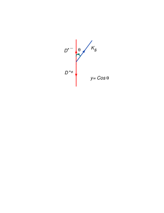
Figure 2: The definition of the variable $y$.

Carrying out the integration over the phase space variables $y$ and $E_{k}$ one gets the following expressions for the time-dependent total rates for $B^{0}(t)\to D^{*+}D^{*-}K_{s}$ and the CP conjugate process,

$$\Gamma(t) = \frac{1}{2}[I_{0}+2\sin(2\beta)\sin(\Delta mt)I_{s1}],$$ (8)

$${\overline{\Gamma}}(t) = \frac{1}{2}[I_{0}-2\sin(2\beta)\sin(\Delta mt)I_{s1}],\$$ (9)

where $I_{0}$ and $I_{s1}$ are the integrated $G_{0}(y,E_{k})$ and $G_{s1}(y,E_{k})$ functions. One can then extract $\sin(2\beta)$ from the rate asymmetry

$$\frac{\Gamma(t)-{\overline{\Gamma}}(t)}{\Gamma(t)+{\overline{\Gamma}}(t)}=D\sin(2\beta)\sin(\Delta mt);\quad D=\frac{2I_{s1}}{I_{0}},\$$ (10)

where $D$ is the dilution factor. Furthermore,

$$I_{0}=2\Gamma(0)=2{\overline{\Gamma}}(0).\$$ (11)

The $\cos(2\beta)$ term can be probed by integrating over half the range of the variable $y$ which can be taken for instance to be $y\geq 0$ for $B$ decay and $y\leq 0$ for ${\bar{B}}$ decay.

$$\frac{{\Gamma}(t,y\geq 0)}{I_{0}}=\quad\quad\quad\ \quad\quad$$

$$\frac{1}{2}[\frac{{J}_{0}}{I_{0}}+\frac{{J}_{c}}{I_{0}}\cos(\Delta mt)+2\sin(2\beta)\sin(\Delta mt)\frac{{J}_{s1}}{I_{0}}$$

$$-2\cos(2\beta)\sin(\Delta mt)\frac{{J}_{s2}}{I_{0}}],$$ (12)

$$\frac{{\overline{\Gamma}}(t,y\leq 0)}{I_{0}}=\quad\quad\quad\ \quad\quad$$

$$\frac{1}{2}[\frac{{J}_{0}}{I_{0}}+\frac{{J}_{c}}{I_{0}}\cos(\Delta mt)-2\sin(2\beta)\sin(\Delta mt)\frac{{J}_{s1}}{I_{0}}$$

$$-2\cos(2\beta)\sin(\Delta mt)\frac{{J}_{s2}}{I_{0}}],\$$ (13)

where ${J}_{0}$, ${J}_{c}$, ${J}_{s1}$ and ${J}_{s2}$, are the integrated $G_{0}(y,E_{k})$, $G_{c}(y,E_{k})$, $G_{s1}(y,E_{k})$ and $G_{s2}(y,E_{k})$ functions integrated over the range $y\geq 0$. One can measure $\cos(2\beta)$ by fitting to the time distribution of ${\Gamma(t)+{\bar{\Gamma}}(t)\over I_{0}}$.

The fits to the data yield babarDDK

$$\frac{J_{c}}{J_{0}} = 0.76\pm 0.18(stat)\pm 0.07(syst),$$

$$\frac{2J_{s1}}{J_{0}}\sin{2\beta} = 0.10\pm 0.24(stat)\pm 0.06(syst),$$

$$\frac{2J_{s2}}{J_{0}}\cos{2\beta} = 0.38\pm 0.24(stat)\pm 0.05(syst).\$$ (14)

Using the theoretical calculation of $\frac{2J_{s2}}{J_{0}}$ browder $\cos{2\beta}$ is preferred to be positive at the 94 % confidence level as the theoretical parameter $J_{s2}/J_{0}$ is positive. It is also interesting to note that $J_{c}/J_{0}$ is significantly different from zero. This implies that there is a sizable resonant contribution to the decay from a unknown $D^{+}_{s1}$ state with large width. This can have important implications for the interpretation of the new $D_{sJ}$ states discovered recently dattapat .

IV $B(t)\to Dh^{0}$

The decay $B(t)\to Dh^{0}$ has been recently proposed to measure $\sin{2\beta}$ and $\cos{2\beta}$ bondar . The idea in this case is also to use intermediate resonances to probe $\cos{2\beta}$. Consider the decays of the $B$ meson to $Dh^{0}(h^{0}=\pi^{0},\eta..)$. The dominant decay is through the $b\to c\bar{u}d$ quark level process.

Figure 3: The decay $B\to Dh^{0}$ .

Next consider the multi body $D$ meson decay. As an example use $D\to K_{s}\pi^{+}\pi^{-}$. We can write,

$$Amp(\bar{D}^{0}\to K_{\scriptscriptstyle S}\pi^{+}\pi^{-}) = f(m_{+}^{2},m_{-}^{2}),$$

$$Amp({D}^{0}\to K_{\scriptscriptstyle S}\pi^{+}\pi^{-}) = f(m_{-}^{2},m_{+}^{2}),$$

$${m_{+,-}}^{2}=(p_{K_{s}}+p_{\pi^{\pm}})^{2}.\$$ (15)

The amplitude for the $B$ decay at time $t_{\rm sig}$ is then given by,

$$M_{\bar{B}^{0}}(\Delta t) = [\bar{B}^{0}\to D^{0}(K_{s}\pi^{+}\pi^{-})h^{0}]C-$$

$$i\frac{p}{q}\eta_{h^{0}}(-1)^{l}[{B}^{0}\to\bar{D}^{0}(K_{s}\pi^{+}\pi^{-})h^{0}]S,$$

(16)

where $C=\cos(\Delta m\Delta t/2)$ and $S=\sin(\Delta m\Delta t/2)$ and

$$M_{\bar{B}^{0}}(\Delta t) = f(m_{-}^{2},m_{+}^{2})C-$$ (17)

$$i\frac{p}{q}\eta_{h^{0}}(-1)^{l}f(m_{+}^{2},m_{-}^{2})S.$$

Then, using Eq. 15,

$$M_{\bar{B}^{0}}(\Delta t) = f(m_{-}^{2},m_{+}^{2})C-$$ (18)

$$ie^{-i2\phi_{1}}\eta_{h^{0}}(-1)^{l}f(m_{+}^{2},m_{-}^{2})S,$$

$$M_{B^{0}}(\Delta t) = f(m_{+}^{2},m_{-}^{2})C-$$ (19)

$$ie^{+i2\phi_{1}}\eta_{h^{0}}(-1)^{l}f(m_{-}^{2},m_{+}^{2})S.$$

One then needs to model $f(m_{+}^{2},m_{-}^{2})$ to extract the phase $2\phi_{1}(2\beta)$. This is done by assuming Breit-Wigner form for the various contributing resonances. A non resonant component is also included. The experimental measurements of this process is discussed in other talks in the workshopkathy .

V $\bar{B}(t)\to D^{(*)}\bar{D}^{(*)}$

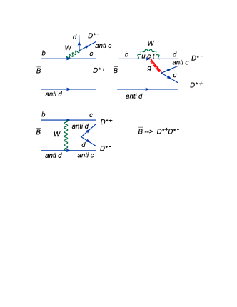
Figure 4: The decay $\bar{B}\to D^{(*)}\bar{D}^{(*)}$ .

The amplitude for $\bar{B}\to D^{(*)}\bar{D}^{(*)}$ can be written as,

$$A^{D} = (T+E+P_{c})V_{cb}^{*}V_{cd}+P_{u}V_{ub}^{*}V_{ud}+$$ (20)

$$(P_{t}+P_{EW}^{C})V_{tb}^{*}V_{td},$$

$$= (T+E+P_{c}-P_{t}-P_{EW}^{C})V_{cb}^{*}V_{cd}$$

$$+(P_{u}-P_{t}-P_{EW}^{C})V_{ub}^{*}V_{ud},$$

$$\equiv {\cal A}_{ct}\ e^{i\delta^{ct}}+{\cal A}_{ut}\ e^{i\gamma}e^{i\delta^{ut}}.$$

The time-dependent measurement of this decay allows one to obtain the three observables,

$$B \equiv \frac{1}{2}\left(|A|^{2}+|{\overline{A}}|^{2}\right)={\cal A}_{ct}^{2}+{\cal A}_{ut}^{2}$$

$$+ 2{\cal A}_{ct}\,{\cal A}_{ut}\cos\delta\cos\gamma,$$

$$a_{dir} \equiv \frac{1}{2}\left(|A|^{2}-|{\overline{A}}|^{2}\right)=-2{\cal A}_{ct}\,{\cal A}_{ut}\sin\delta\sin\gamma,$$

$$a_{indir} \equiv {\rm Im}\left(e^{-2i\beta}A^{*}{\overline{A}}\right)$$ (21)

$$- {\cal A}_{ct}^{2}\sin 2\beta-2{\cal A}_{ct}\,{\cal A}_{ut}\cos\delta\sin(2\beta+\gamma)$$

$$- {\cal A}_{ut}^{2}\sin(2\beta+2\gamma).\$$

The three independent observables depend on five theoretical parameters: ${\cal A}_{ut}$, ${\cal A}_{ct}$, $\delta$, $\beta$, $\gamma$. If ${\cal A}_{ut}$ can be neglected then one can obtain $\sin{2\beta}$. In general, however, one cannot obtain CP phase information from these measurements- this is the well known penguin pollution problem. Hence theoretical input is necessary to get the CKM phase information. One can partially solve for the theory amplitudes as,

$${\cal A}_{ct}^{2} = {a_{R}\cos(2\beta+2\gamma)-a_{indir}\sin(2\beta+2\gamma)-B\over\cos 2\gamma-1},$$

$$a_{R}^{2} = B^{2}-a_{dir}^{2}-a_{indir}^{2}~{}.$$ (22)

One can then obtain ${\cal A}_{ct}$ from a partner process and use it as a theory input. We can then obtain $\gamma$ if given $\beta$ and vice versa. The partner process can be chosen to be $\bar{B}\to{D}^{(*)}\bar{D}_{s}^{(*)}$ justin or $\bar{B_{s}}\to{D}_{s}^{(*)}\bar{D}_{s}^{(*)}$ fleischer .

VI Conclusions

The measurement of both $\sin{2\beta}$ and $\cos{2\beta}$ is crucial to test the standard model predictions of CP violation. This is all the more important as there are several decays where there are hints of beyond standard model physicsdattanp , making the precise measurements of the CKM angles a top priority. In this talk we have described several decays involving B decays to charm that probe both $\sin{2\beta}$ and $\cos{2\beta}$.

References

(1)
See for example,
R. Fleischer, G. Isidori and J. Matias,
JHEP 0305, 053 (2003)
[arXiv:hep-ph/0302229].
(2)
B. Aubert et al. [BABAR Collaboration],
Phys. Rev. D 71, 032005 (2005)
[arXiv:hep-ex/0411016].
(3)
A. Datta and D. London,
Int. J. Mod. Phys. A 19, 2505 (2004)
[arXiv:hep-ph/0303159].
(4)
T. E. Browder, A. Datta, P. J. O’Donnell and S. Pakvasa,
Phys. Rev. D 61, 054009 (2000)
[arXiv:hep-ph/9905425];
For earlier papers see:J. Charles, A. Le Yaouanc, L. Oliver, O. Pene and J. C. Raynal,
Phys. Lett. B 425, 375 (1998)
[Erratum-ibid. B 433, 441 (1998)]
[arXiv:hep-ph/9801363];
P. Colangelo, F. De Fazio, G. Nardulli, N. Paver and Riazuddin,
Phys. Rev. D 60, 033002 (1999)
[arXiv:hep-ph/9901264].
(5)
B. Aubert et al. [BABAR Collaboration],
Phys. Rev. D 74, 091101 (2006)
[arXiv:hep-ex/0608016].
(6)
A. Datta,
Int. J. Mod. Phys. A 19, 5501 (2004)
[arXiv:hep-ph/0407330];
A. Datta and P. J. O’donnell,
Phys. Lett. B 572, 164 (2003)
[arXiv:hep-ph/0307106];
A. Datta and P. J. O’Donnell,
Phys. Lett. B 567, 273 (2003)
[arXiv:hep-ph/0306097].
(7)
A. Bondar, T. Gershon and P. Krokovny,
Phys. Lett. B 624, 1 (2005)
[arXiv:hep-ph/0503174].
(8)
See for instance,
K. A. George,
arXiv:hep-ex/0701044.
(9)
J. Albert, A. Datta and D. London,
Phys. Lett. B 605, 335 (2005)
[arXiv:hep-ph/0410015];
A. Datta and D. London,
Phys. Lett. B 584, 81 (2004)
[arXiv:hep-ph/0310252].
(10)
R. Fleischer,
Eur. Phys. J. C 10, 299 (1999)
[arXiv:hep-ph/9903455].
(11)
See for instance,
S. Baek, A. Datta, P. Hamel, O. F. Hernandez and D. London,
Phys. Rev. D 72, 094008 (2005)
[arXiv:hep-ph/0508149];
S. Baek, P. Hamel, D. London, A. Datta and D. A. Suprun,
Phys. Rev. D 71, 057502 (2005)
[arXiv:hep-ph/0412086];
A. Datta, M. Imbeault, D. London, V. Page, N. Sinha and R. Sinha,
Phys. Rev. D 71, 096002 (2005)
[arXiv:hep-ph/0406192];
A. Datta and D. London,
Phys. Lett. B 595, 453 (2004)
[arXiv:hep-ph/0404130];
A. Datta,
Phys. Rev. D 66, 071702 (2002)
[arXiv:hep-ph/0208016];
A. Datta, X. G. He and S. Pakvasa,
Phys. Lett. B 419, 369 (1998)
[arXiv:hep-ph/9707259];
T. E. Browder, A. Datta, X. G. He and S. Pakvasa,
Phys. Rev. D 57, 6829 (1998)
[arXiv:hep-ph/9705320].