ANL-HEP-PR-07-14, MSU-HEP-07012

The Strange Parton Distribution of the Nucleon:
Global Analysis and Applications

H.L. Lai^a,b,c, P. Nadolsky^d, J. Pumplin^a, D. Stump^a,
W.K. Tung^a,b, C.-P. Yuan^a

^a Michigan State University, E. Lansing, MI, USA

^b University of Washington, Seattle, WA, USA

^c Taipei Municipal University of Education, Taipei, Taiwan

^d Argonne National Laboratory, Argonne, IL, USA

The strangeness degrees of freedom in the parton structure of the nucleon are explored in the global analysis framework, using the new CTEQ6.5 implementation of the general mass perturbative QCD formalism of Collins. We systematically determine the constraining power of available hard scattering experimental data on the magnitude and shape of the strange quark and anti-quark parton distributions. We find that current data favor a distinct shape of the strange sea compared to the isoscalar non-strange sea. A new reference parton distribution set, CTEQ6.5S0, and representative sets spanning the allowed ranges of magnitude and shape of the strange distributions, are presented. Some applications to physical processes of current interest in hadron collider phenomenology are discussed.

1 Introduction

Although the global analysis of parton distribution functions (PDFs) has been in progress for over two decades, certain components of the parton structure of the nucleon are still poorly determined [1, 2]. Foremost among these, perhaps surprisingly, is the strangeness sector. The lack of knowledge on the strange and anti-strange parton distributions, $s(x)$ and $\bar{s}(x)$, is reflected in the common practice in current global QCD analyses of PDFs of adopting the simplifying ansatz $s=\bar{s}=r\,(\bar{u}+\bar{d})/2$ (where $\bar{u}$ and $\bar{d}$ are the up and down sea anti-quarks) at some low factorization scale. Even the proportionality constant $r$ is only very loosely constrained by data.

Progress in incorporating heavy quark mass effects into the general PQCD formalism, combined with recent precision cross section data from HERA and fixed-target experiments, provides us with an opportunity to re-assess the situation. This is important theoretically, because the parton structure of the nucleon, including strangeness, is a fundamental aspect of QCD dynamics at the confinement scale. It is also important phenomenologically, because $s(x)$ and $\bar{s}(x)$ are significant for quantitative calculations of certain key short-distance processes at hadron colliders.

In a recent paper [3], hereafter referred to as CTEQ6.5M, we investigated how the up/down-quark and the gluon distributions, and their uncertainties, are affected by the new theoretical and experimental input, while keeping the conventional $s=\bar{s}\propto(\bar{u}+\bar{d})$ ansatz. We found that the new developments give rise to notable shifts in the PDFs which have a significant impact on hadron collider phenomenology. In this work, we extend the analysis to focus on the strangeness sector. Specifically, we explore to what extent we can now quantify $s(x)$ and $\bar{s}(x)$ without restricting their shapes; and then consider some implications of the improved PDFs on the phenomenology of Standard Model (SM) and Beyond Standard Model (BSM) physics at the Tevatron and the LHC.

In Section 2, we discuss issues relevant to performing global QCD analysis with a focus on the strangeness sector. In Section 3, we study the symmetric strange sea combination $s(x)+\bar{s}(x)$. We determine the number of new strangeness parameters that can be constrained by current data, present an improved PDF set CTEQ6.5S0 that best represents the global data, and investigate the ranges of the magnitude and shape of the symmetric strange sea allowed by the available constraints. Several PDF sets that exemplify these ranges, CTEQ6.5Si ($i=1,\dots,4$), are given. In Section 4, we examine the strangeness asymmetry function $s(x)-\bar{s}(x)$. We discuss constraints that can be placed on this function by current global analysis, and compare the results with existing ones. To illustrate the use of these new results, we consider in Section 5 implications of the new PDFs on: (i) the SM process $p\,p\mkern-11.0mu^{\scriptscriptstyle{(-)}}\to g\,+\,\bar{s}\to W^{+}\,+\,c$; and the BSM process $p\,p\mkern-11.0mu^{\scriptscriptstyle{(-)}}\to\bar{s}\,+\,c\to H^{+}$. In Section 6, we summarize our results.

2 Global Analysis with Focus on the Strange Sector

The staple input to standard global QCD analyses of PDFs are the total inclusive cross sections in deep inelastic scattering (DIS), Drell-Yan processes (DY), and inclusive jet production. These processes are largely insensitive to the strange content of the nucleon, since the contributions from the non-stange sea-quarks and gluon partons are larger and are of similar shape to the strange sea distribution. In principle, at leading order (LO) in QCD, the neutral current (NC) and charged current (CC) DIS structure functions depend on somewhat different combinations of strange and non-strange partons. Therefore certain specific combinations of these structure functions can be sensitive to $s(x)$ and $\bar{s}(x)$. But in practice, due to the large uncertainties inherent in combining data from different kinds of experiments (CC vs. NC), the constraints on strange and anti-strange PDFs provided by total inclusive data are known to be very weak, as we will also see quantitatively in this paper.

The semi-inclusive CC process $\nu/\bar{\nu}\,+\,N\to\mu^{-/+}\,+\,H_{c}\,+\,X$ (where $N$ denotes a nucleon or nucleus and $H_{c}$ a charm meson or baryon) is sensitive to strange distributions through the LO partonic process $W^{+}\,+\,s\to c$, where $c$ is the charm quark. The experimental signature of this process is dimuon production in neutrino (anti-neutrino) scattering, since the semi-leptonic decay of the charm meson gives rise to a second muon in the final state [4]. Our study is partly motivated by the recent availability of the final analysis of the high statistics NuTeV measurement of this process [6].

The task of reliably constraining $s(x)$ and $\bar{s}(x)$ must be performed, however, within the context of a comprehensive global QCD analysis. This is because, beyond the LO in perturbative theory, QCD dynamics strongly couples the strange degrees of freedom to the gluon and the other quark flavors. No parton flavor can be determined in isolation: all available high precision inclusive data that constrain the light degrees of freedom are needed in the analysis. Furthermore, the charm final state in the dimuon production process requires that heavy quark mass effects be included properly. Thus, a consistent formalism incorporating mass effects in both QCD factorization (dynamics) and in the phase space treatment (kinematics) must be applied to all the relevant DIS processes in the global analysis. The global analysis framework of CTEQ6.5 [3] contains these features, and thus provides a suitable basis for performing this study.

It is convenient to work with symmetric and anti-symmetric combinations of $s$ and $\bar{s}$:

$$s_{{}^{\pm}}(x,\mu)\,\equiv\,s(x,\mu)\,\pm\,\bar{s}(x,\mu)\;.$$ (1)

These have opposite CP properties and evolve differently under QCD evolution. In Ref. [3], the conventional ansatz

$$s_{+}(x) = r[\bar{u}(x)+\bar{d}(x)]$$ (2)

$$s_{-}(x) = 0$$ (3)

at the initial scale $\mu=Q_{0}=1.3\,\mathrm{GeV}$ was made. In this common approach, the only parameter associated with the strangeness degree of freedom is the constant ratio $r$ of the strange to non-strange sea distributions at $Q_{0}$.

In the current work, we extend the analysis to include additional independent parameters characterizing the shape of the strangeness distributions, and study their effect on the global fit. The number of new parameters and the associated functional forms will be specified in subsequent sections devoted to $s_{+}(x)$ and $s_{-}(x)$.

The experimental input to this study is essentially the same as in the CTEQ6.5M analysis [3]. It consists of the full range of HERA I NC and CC total cross section and semi-inclusive charm and bottom production data, along with standard fixed-target NC and CC DIS and DY experiments, and the Tevatron measurements of inclusive jet production and the charge asymmetry of leptons from $W$ production. Correlated systematic errors, whenever available, are incorporated in the analysis.

Since the neutrino dimuon cross sections are of special importance in exploring the strangeness degrees of freedom, we include both the CCFR and the NuTeV data sets [4] for this analysis. The measured “forward dimuon production” cross sections from [4] cannot be directly compared to our theoretical calculation of inclusive charm production cross section, because they also depend on the fragmentation of the charm quark into charmed particles, and the decay of those particles. We rely on the results of the recent comprehensive analysis of Mason [6] to make the connection between the two.

In the global analysis of PDFs, the parton degrees of freedom must be matched to the constraining power of the available input experimental data within the adopted theoretical framework, in order for the results to be meaningful. The first question in studying the strangeness sector of the nucleon parton structure must therefore be: are current theory and experiment able to discern independent non-perturbative strange degrees of freedom; and, if so, how many such degrees of freedom are needed?

We shall try to answer this question by comparing global fits of the conventional type (with no independent strange parton degrees of freedom except the overall normalization) to new fits obtained with various numbers of new strangeness shape parameters. The reference PDF set, with the conventional ansatz (2)–(3) imposed at $\mu=Q_{0}=1.3\,\mathrm{GeV}$, is essentially CTEQ6.5M [3].

3 The Symmetric Strange Sea $\mathbf{s_{+}(x)}$

To extend the analysis to the strangeness sector of parton parameter space, we first examine the symmetric component of the strange sea, $s_{+}(x)$. For the non-perturbative input distribution, we adopt the standard initial form

$$s_{+}(x,Q_{0})=A_{0}\,x^{A_{1}}\,(1-x)^{A_{2}}\,P_{+}(x)\ \ ,$$ (4)

where $P_{+}(x)$ is a smooth positive definite function on the interval $(0,1)$. The function $P_{+}(x)$ depends on additional parameters $A_{3},\dots$ as needed. The normalization constant $A_{0}$ which controls the overall magnitude of the strange distribution is related to the strange/non-strange ratio parameter $r$ in Eq. (2), and hence it will not be counted as a new parameter. The parameters $A_{1},A_{2},\dots$ define the shape of the non-perturbative strange distribution $s_{+}(x,Q_{0})$. Because the experimental constraints on the new parameters are not tight, we generally retain the relation $A_{1}^{s_{+}}=A_{1}^{\bar{u}+\bar{d}}$, suggested by common Regge considerations for small-$x$ behavior of PDFs, to reduce arbitrariness. This leaves $A_{2},A_{3},\dots$ as the new strangeness parameters to be investigated in the rest of this section.

3.1 The Number of New Shape Parameters

We have examined the quality of global fits obtained with a variety of functional forms for $P_{+}(x)$ that involve new shape parameters, compared to CTEQ6.5M which is taken as a reference fit with $s_{+}\propto(\bar{d}+\bar{u})$. The main results are summarized in Table 1, which shows the reduction in $\chi^{2}$ with respect to CTEQ6.5M (hence the improvement in the goodness-of-fit) for the full data set $\Delta\chi_{\mathrm{global}}^{2}$ and for the dimuon data sets $\Delta\chi_{\mu^{+}\mu^{-}}^{2}$, when $1$, $2$, or $3$ new strangeness parameters are added to the global fit. The $1$ new parameter case—with $A_{2}$ only—corresponds to $P_{+}=1$ in Eq. (4); the other cases involve various choices of non-trivial functions $P_{+}(x)$.

change of	# new parameters
goodness-of-fit	1	2	3
$-\Delta\chi_{\mathrm{global}}^{2}$ (3542 pts.)	65	68	69
$-\Delta\chi_{\mu^{+}\mu^{-}}^{2}$ (149 pts.)	46	48	50

Table 1: Reduction in $\chi^{2}$’s with respect to the reference fit CTEQ6.5M due to the introduction of new $s_{+}(x)$ strangeness degrees of freedom.

We see that whereas, at first sight, the significance of $\Delta\chi_{\mathrm{global}}^{2}\sim 67$ for the full global data set of $3542$ points may be arguable, it is striking that the bulk of this reduction is concentrated in the most physically relevant $\nu$ and $\bar{\nu}$ dimuon data sets. The improvement in the goodness-of-fit for the dimuon data sets—$\Delta\chi_{\mu^{+}\mu^{-}}^{2}\sim 48$—is quite significant, because, for 149 data points, the normal 90% confidence level criterion corresponds to a $\Delta\chi^{2}$ of 22. Our general analysis procedure, as described in more detail in [3], requires acceptable fits to be within the 90% confidence levels of all contributing data sets. In the current study, the deciding factor is therefore the goodness-of-fit of the dimuon data sets. This was already anticipated in Sec. 2. Fig. 1 gives a graphical illustration of the improvement on the fit to the more accurate neutrino dimuon data sets using a new PDF set with (minimal) independent strangeness sector (cf. next subsection) compared to that using CTEQ6.5M.

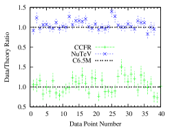
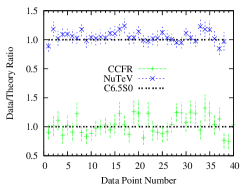
Figure 1: Comparison of neutrino dimuon data to fits using CTEQ6.5M (left panel) and the new set CTEQ6.5S0 of Sec. 3.2 (right panel). The data points are sorted in $y$-bins, and within each $y$-bin, by $x$ value, and then $Q$ value.

We conclude from these results that the current global analysis strongly favors a different shape for the strange sea $s_{+}(x)$, compared to the (isoscalar) non-strange sea $\bar{u}(x)+\bar{d}(x)$. From the physics point of view, this is only natural, since the initial parton distributions reflect low energy non-perturbative physics. QCD dynamics at long distances does differentiate the strange and non-strange sectors, as seen in hadron spectroscopy. The conventional ansatz of the same shape but different sizes for the initial parton distributions has been only a convenient working ansatz in the absence of sufficient experimental constraints on the difference. The results presented above show that recent improvements in theory and experiment now allow us to discern the difference.

However, Table 1 also shows the limitation of current experimental constraints: there is no significant improvement in the goodness-of-fit when the number of new degrees of freedom is increased beyond 1. This means our global analysis cannot distinguish the simple shape

$$s_{+}(x,Q_{0})=A_{0}\,x^{A_{1}}(1-x)^{A_{2}}$$ (5)

from more complex forms that invoke additional parameters ($P_{+}(x;\,A_{3},A_{4},A_{5})\neq 1$ in Eq. (4)). Because of this, Eq. (5) will suffice as a starting point for exploring the strangeness sector of parton parameter space.

3.2 New Central PDF set, CTEQ6.5S0

With the independent strangeness sector represented by the input function (5), we need to establish a new reference PDF set that provides the best fit to the current global hard scattering data. This set will be referred to as CTEQ6.5S0 in subsequent discussions. It represents an improvement of the CTEQ6.5M PDF set of [3] as discussed in the last subsection. Except for the differentiation between $s_{+}(x)$ and $\bar{u}(x)+\bar{d}(x)$ shapes, these two PDF sets are very similar to each other.

In Fig. 2 we compare the sea distributions from the two PDF sets. The $x$-axis is scaled as $x^{1/3}$ so that the large-$x$ and small-$x$ regions are both clearly displayed. The $y$-axis is scaled so that the area under each curve is proportional to the momentum fraction carried by that PDF. We see that the isoscalar non-strange sea $\bar{u}(x)+\bar{d}(x)$ is almost unchanged, while the new CTEQ6.5S0 symmetric strange sea $s_{+}(x)$ has become somewhat smaller and softer compared to CTEQ6.5M.

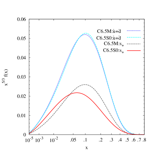
Figure 2: The new CTEQ6.5S0 $s_{+}(x)$ and $\bar{u}(x)+\bar{d}(x)$ PDFs at $\mu=1.3\ \mathrm{GeV}$ compared to those of CTEQ6.5M.

3.3 Constraints on the Magnitude of $s_{+}$

The “magnitude” of a parton flavor $f$ ($=g,u,\bar{u},d,\bar{d},s,\bar{s},...$) inside the nucleon is naturally represented by the momentum fraction it carries:

$$\langle x\rangle_{f}\equiv\int_{0}^{1}x\,f(x)\,dx\ \ .$$ (6)

By this measure, the value of $\langle x\rangle_{s_{+}}$ for the reference CTEQ6.5S0 set is $0.027$, while for CTEQ6.5M it was $0.032$.

To study the uncertainty in the magnitude of $s_{+}$, we performed a series of global fits using the Lagrange Multiplier method of [7, 8] to map out the allowed range of $\langle x\rangle_{s_{+}}$. Keeping in mind the results of Sec. 3.1, as the value of $\langle x\rangle_{s_{+}}$ is varied around the central value $0.027$, we keep track of the variation in overall $\chi_{\mathrm{global}}^{2}$ as well as the variation in $\chi_{\mu^{-}\mu^{+}}^{2}$. The results are presented in Fig. 3.

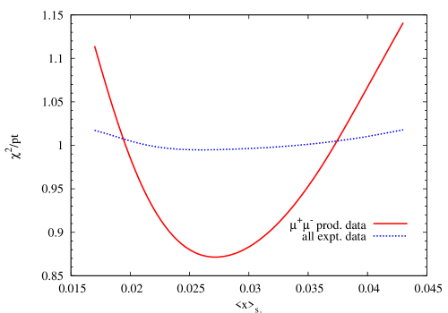
Figure 3: $\chi^{2}$ per data point vs. $\langle x\rangle_{s_{+}}$ for the full data set (3542 points) and for the $\nu$ and $\bar{\nu}$ dimuon production data (149 points).

For convenience, the comparison is made on $\chi^{2}$ per data point, with the number of data points being given in Table 1. We see that, as expected, the $\nu$ and $\bar{\nu}$ dimuon data sets are quite sensitive to the magnitude of the strangeness PDFs, whereas the rest of the global data sets are basically insensitive to it.

Thus, the experimental constraints on $\langle x\rangle_{s_{+}}$ are provided essentially by the $\nu$ and $\bar{\nu}$ dimuon data sets.  Following Refs. [9, 3], we determine the uncertainty range of $\langle x\rangle_{s_{+}}$ by the 90% confidence criteria on the dimuon production data sets. This range is $0.018\,<\langle x\rangle_{s_{+}}<\,0.040\,$. The two sets of PDFs that represent the best fits corresponding to the lower (upper) bound value of $\langle x\rangle_{s_{+}}$ will be referred to as CTEQ6.5S1 (CTEQ6.5S2). The variation of $\langle x\rangle_{s_{+}}$ is strongly correlated with the normalization of the $\nu$ and $\bar{\nu}$ dimuon production data sets compared to the theoretically calculated inclusive charm production cross section. There are various sources of uncertainty on this overall factor: experimental (global and energy-dependent) normalization of the total cross sections ($\sim 2-5\%$), fragmentation function of charm quark to charmed hadrons, branching ratio of charmed hadron decay to muon ($\sim 10\%$), …, etc. These are taken into account according to our standard uncertainty analysis. The limits of $\langle x\rangle_{s_{+}}$ obtained above correspond to $\pm 20\%$ ovreall variation of the normalization factor, as determined by this analysis procedure. As the magnitude of $\langle x\rangle_{s_{+}}$ varies, the shape of $s_{+}(x)$ also adjusts to best fit the global data. A plot of $s_{+}(x)$ for these PDFs will be shown in the next section.

The relative strength of the strange partons is conveniently characterized by the ratio of $\langle x\rangle_{s+\bar{s}}$ to the average of strange and non-strange sea $\kappa\equiv 3\langle x\rangle_{s+\bar{s}}/(2\langle x\rangle_{\bar{u}+\bar{d}}+\langle x\rangle_{s+\bar{s}})$ (Note, $u_{\mathrm{sea}}=\bar{u}$, $d_{\mathrm{sea}}=\bar{d}$.) The values of $\kappa$ for CTEQ6.5Si, $i=1,0,\,2$, are $0.35,\,0.54,\,0.75,$ respectively. The relative size of the strange and non-strange distributions can also be expressed in terms of the ratio of strange to non-strange sea, $r=\langle x\rangle_{s+\bar{s}}/\langle x\rangle_{\bar{u}+\bar{d}}=2\kappa/(3-\kappa)$. This is a generalization of the ratio parameter introduced in Eq. (2) for the special case of the same shape for strange and non-strange seas. The PDF sets CTEQ6.5Si, $i=1,\,0,\,2$, correspond to $r=0.27,\,0.44,0.67$, respectively; while $r=0.50$ for CTEQ6.5M.

3.4 Constraints on the Shape of $s_{+}(x)$

It is also of interest to ask what is the uncertainty in the shape of the input $s_{+}(x)$. To study this, we need to expand the input functional form beyond the minimal one given in Eq. (5). As shown in Table 1, fits obtained with $P_{+}(x)$ in Eq. (4) that contain additional parameters will have comparable goodness-of-fit to current data compared with those described above (with $P_{+}(x)=1$). The variation of the $s_{+}(x)$ shape among fits obtained with expanded parametrizations should therefore give a reasonable measure of the range allowed by existing data.

To carry out this study, we explored a variety of choices for $P_{+}(x;A_{3},A_{4})$ and examined the shape of $s_{+}(x)$ for candidate fits within the 90% confidence level constraints of the dimuon data sets. (The goodness-of-fit to the majority inclusive data sets was again insensitive to these variations, staying consistently close to the optimal level.) It is difficult to uniquely characterize the “shape” of a function such as $s_{+}(x)$ when the experimental constraints are relatively weak. We have chosen two representative alternative PDF sets among those explored just to illustrate the range allowed by the 90% confidence level criterion. These will be referred to as CTEQ6.5S3 and CTEQ6.5S4.

Figure 4 shows the strangeness distribution $s_{+}(x)$ at the initial scale $\mu=1.3\,\mathrm{GeV}$ for the five PDF sets, CTEQ6.5Si, $i=0,...,4$. The axes are scaled the same way as in Fig. 2. The area under each curve corresponds to the momentum fraction carried by $s_{+}$, hence directly illustrates its magnitude. The solid (red) curve shows the reference PDF set CTEQ6.5S0. The other curves illustrate the range of variation of the magnitude and shape of $s_{+}(x)$ allowed by current data.

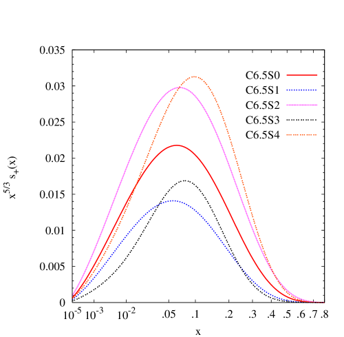
Figure 4: The strangeness distribution $s_{+}(x)$ at the initial scale $\mu=1.3\,\mathrm{GeV}$ for the five PDF sets CTEQ6.5Si, $i=0,\dots,4$.

4 The Strangeness Asymmetry $\mathbf{s_{-}(x)}$

To study the anti-symmetric combination $s_{-}(x)$, the strangeness asymmetry function, we must bear in mind that (i) if we want to keep both $s$ and $\bar{s}$ parton distributions positive definite, it is necessary to maintain the condition $|s_{-}|\leq|s_{+}|$; and (ii) in order to satisfy the strangeness quark number sum rule, we must have $\int_{0}^{1}s_{-}(x)dx=0$. The latter condition implies that $s_{-}(x)$ changes sign at least once in the interval $0<x<1$. Current data do not have enough discriminating power to establish multiple oscillatory behavior of $s_{-}(x)$, so we shall restrict the parametrization of $s_{-}(x)$ to the case of a single crossing of the $x$-axis.

A convenient smooth parametrization that has the required features is

$$s_{-}(x,Q_{0})=s_{+}(x,Q_{0})\frac{2}{\pi}\tan^{-1}[\,c\,x^{a}(1-\frac{x}{b})\,e^{dx+ex^{2}}]$$ (7)

where $c$ controls the sign and the overall magnitude of $s_{-}(x)$, $a$ characterizes the difference in small-$x$ behavior between $s_{-}(x)$ and $s_{+}(x)$ (expected on physical grounds), $b$ represents the $x$-value at which $s_{-}(x)$ changes sign, and the factor $e^{dx+ex^{2}}$ may be included if needed to provide more flexibility in the shape of the function. We see that, in order to have a non-trivial strangeness asymmetry, a minimum of 3 parameters—$a,b,c$ in Eq. (7)—are required to characterize the non-perturbative input function.

The exploration of the strangeness asymmetry sector can be pursued by the same procedure as for $s_{+}(x)$. The experimental constraints are again expected to come mostly from the $\nu$ and $\bar{\nu}$ dimuon production data sets.

change of	# of parameters
goodness-of-fit	3	4	5
$-\Delta\chi_{\mathrm{global}}^{2}$ (3542 pts.)	15	16	16
$-\Delta\chi_{\mu^{+}\mu^{-}}^{2}$ (149 pts.)	15	15	16

Table 2: Reduction in $\chi^{2}$ with respect to the reference fit CTEQ6.5S0 due to the introduction of strangeness asymmetry parameters.

The results of an extensive study are summarized in Table 2. This time we use CTEQ6.5S0 as the reference fit, and examine the improvement in goodness-of-fit due to the introduction of $3$ (the minimum) to $5$ parameters to characterize strangeness asymmetry degrees of freedom. The $3$-parameter case refers to the set $a,b,c$; and the other cases add the parameters $d,e$ in order. The numbers given in this table are not unique since many equivalent examples have been studied; they are representative of the general pattern.

Significance of non-zero Strangeness Asymmetry:

Compared to the case of $s_{+}$ (Table 1), we see that the reductions in $\chi_{\mathrm{global}}^{2}$ (with respect to CTEQ6.5S0 which has a symmetric strangeness sea) are insignificant (for the total number of points), and all the reductions come from the dimuon data sets. Furthermore, the numbers for $\Delta\chi_{\mu^{+}\mu^{-}}^{2}$ are a factor of 3 smaller than those appearing in Table 1; and are below the 90% C.L. figure of 22. Thus, we consider the improvement on the goodness-of-fit over the no strangeness asymmetry case to be marginal. This does not mean, however, that experimental evidence is against the existence of strangeness asymmetry! To the contrary, the latter can be sizable since the constraints are shown to be weak. Thus, in the next subsection, we shall investigate the allowed range of this asymmetry, assuming it is non-zero.

One feature of these fits is worth noting: the fitted value for the $\,a\,$ parameter of Eq. (7), if let free, is generally in the range of the theoretical expectation $\sim 0.5$—the difference of the two Regge intercepts of the CP even and odd trajectories. In view of this fact, in further studies described below, we normally set $a=0.5$ and let the other parameters vary, in order to render the very loosely constrainted fits more stable.

The magnitude of strangeness asymmetry can again be characterized by the first moment of $s_{-}$: $\langle x\rangle_{s_{-}}=\int_{0}^{1}x\,s_{-}(x,Q_{0})\,dx$. The best fit to global data, using the minimal parametrization ($d\!=\!e\!=\!0$ in Eq. (7)), corresponds to $\langle x\rangle_{s_{-}}=0.0018$. This value is completely consistent with those of the previous global analysis [10] and with the recent final experimental analysis of the NuTeV dimuon data alone [6].

Range of Allowed Strangeness Asymmetry:

The uncertainties of the magnitude and shape of $s_{-}(x)$ can again be studied using the Lagrange Multiplier method. Applying the 90% confidence criterion, we estimate the range of the magnitude to be $-0.001<\langle x\rangle_{s_{-}}<0.005$. This range again coincides with that found in [10].

We note that $s_{-}(x)$ is particularly sensitive to the difference between the $\nu$ and $\bar{\nu}$ cross sections. In our analysis, we treat the overall normalization of the NuTeV $\nu$ and $\bar{\nu}$ dimuon data sets as a fitting parameter (as already mentioned in Sec. 3), but keep the relative normalization between these data sets fixed. If this relative normalization were allowed to float, both the magnitude and the shape of $s_{-}(x)$ would change significantly (along with a reduction in $\chi^{2}$’s that is larger than those shown in Table 2).

In view of the large range of uncertainty on $\langle x\rangle_{s_{-}}$, which includes the possibility of zero asymmetry, we do not think a strong statement can be made about the strangeness asymmetry. However, the results of existing phenomenological studies (Refs. [10, 6] as well as the present work) and physical considerations (e.g. the light-cone wavefunction models [11]) all suggest that $\langle x\rangle_{s_{-}}$ is most likely positive. Figure 5 illustrates typical shapes of the asymmetry function $s_{-}(x)$ and the corresponding momentum distribution $x\,s_{-}(x)$. The central curve (solid line) corresponds to the best fit; the two extreme curves represent the two limiting cases corresponding to the lower and upper bounds of $\langle x\rangle_{s_{-}}$ described above; and the other two provide alternative examples. These choices represent different possible small-$x$ behaviors that span the entire physically allowed range, not just that conforming to the Regge lore.

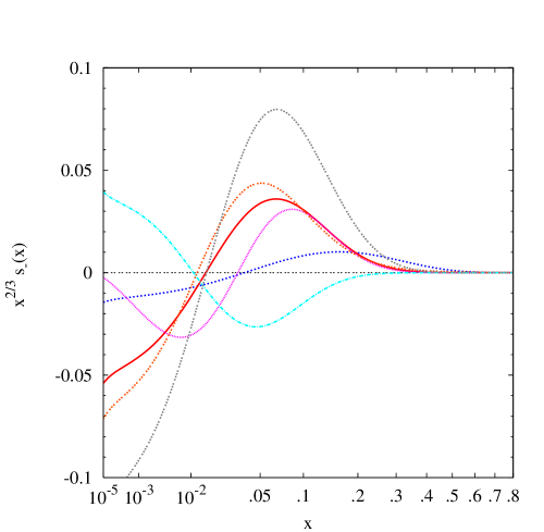
Figure 5: Examples of strangeness asymmetry function $s_{-}(x)$ that are consistent with existing experimental data (left panel); and the corresponding momentum distribution $x\,s_{-}(x)$ (right panel).

5 Physical Applications

The variations of $s(x)$ and $\bar{s}(x)$ found in the previous sections will affect predictions for physical processes that are sensitive to the strange parton distributions. In this section, we will describe two examples: one within and one beyond the SM. A more thorough study will be the subject of a separate paper [12].

$W+c$ production and the strangeness distribution

The inclusive cross section for the hadron collider process $pp\mkern-11.0mu^{\scriptscriptstyle{(-)}}\to W+c+X$ is sensitive to the strange parton distributions through the LO partonic process $g\,\,{s}\to W\,{c}$ [13, 1], where $W$ stands for $W^{\pm}$; $c$, $s$ for the corresponding quark or antiquark. Consider the rapidity distribution $d\sigma/dy$ of the $W^{+}$ boson with the constraint $q_{T}>20$ GeV on the transverse momentum of the outgoing $W^{+}$ boson in the LO approximation (order $\alpha_{s}$). The cross section can be calculated neglecting quark masses in the Wilson coefficient, since these are very small compared to the typical energy scale of the $W^{+}{\bar{c}}$ system. The range of variation of $d\sigma/dy$ for Tevatron Run-2, using the CTEQ6.5Si input PDFs ($i=0-4$), is shown in Fig. 6(a). The cross section in the central rapidity region varies by $\sim 30\%$ among the candidate PDFs. This exceeds the PDF uncertainty estimate obtained using the CTEQ6.5 eigenvector sets (all of which assume the ansatz ( 2) with a fixed $r=0.5$).

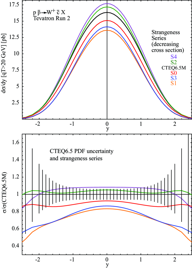
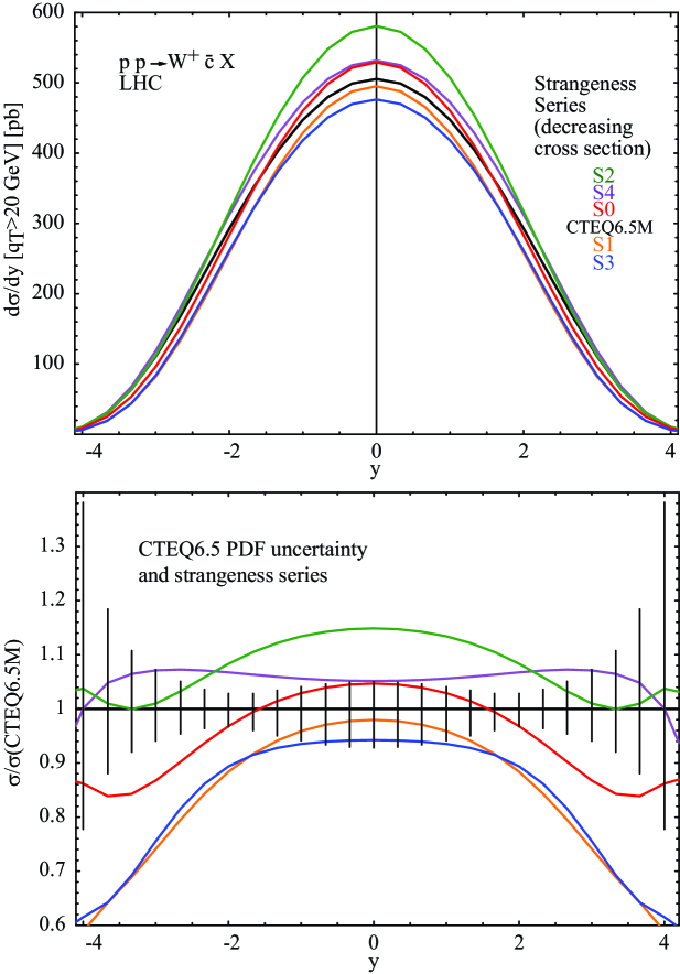
      (a)                                                                       (b)

Figure 6: The rapidity distribution $d\sigma/dy$ at $q_{T}>20$ GeV (top panel) and its fractional uncertainty (bottom panel) at the Tevatron Run-2 (left) and the LHC (right).

This suggests that the measurement of this cross section at the Tevatron will provide useful constraints on the strange distribution.

To make a more realistic feasibility study, it will be necessary to include higher-order QCD contributions, detector acceptance corrections, and background estimates. Here we shall only briefly examine how NLO QCD corrections can be expected to affect the above results. The calculation is carried out by adapting the $\mathcal{O}(\alpha_{s}^{2})$ cross section formulas for high-$q_{T}$ $W$ boson production from Ref. [14]. The most important higher-order contributions to the PDF uncertainty estimate come from the 1-loop corrections to the subprocess $g\,{\bar{s}}\to W^{+}\,{\bar{c}}$, and the tree-level $2\to 3$ process $g\,g\to s\,W^{+}\,{\bar{c}}$. (Our NLO contributions are computed with the constraint $q_{T}>20\,\mathrm{GeV}$ only and may slightly overestimate the NLO rate if a lower cut is imposed on $p_{T}^{c}$ to experimentally identify the $c$-quark jet.) The results are well represented by an overall multiplicative factor of about 1.3 applied to the LO rapidity distributions shown in Fig. 6, for all PDF sets. Hence, the NLO correction preserves sensitivity of the inclusive rapidity distribution to the strange PDF.

Figure 6(b) shows the results of a similar calculation for inclusive $W^{+}\,{\bar{c}}$ production at the LHC. We see that the range of variation of the cross section is more modest in this case. This is because the relevant $x$-range for the LHC has a smaller variation of the strangeness PDFs (see Fig. 4).

Charged Higgs boson production, strangeness, and intrinsic charm

The production of a charged Higgs boson $H^{+}$ via the partonic process $c+{\bar{s}}\to H^{+}$ provides an example of a BSM process that is sensitive to the strange PDF. A charged Higgs field arises in many models where electroweak symmetry breaking involves two or more doublets of Higgs bosons. We shall consider specifically the Type-2 two Higgs doublet model [15]. The $c\,\bar{s}\to H^{+}$ amplitude is enhanced compared to other quark flavors by relatively large $\overline{MS}$ quark masses $\overline{m}_{s}$ and $\overline{m}_{c}$, substantial magnitudes of antistrange and charm PDFs, and the nearly maximal CKM matrix element $V_{cs}\approx 1$. To illustrate the range of variation in predictions for this process at both the Tevatron and the LHC, we compute the on-shell $H^{+}$ production cross section as a function of $M_{H^{+}}$. The calculation includes the NLO QCD correction [16] and is evaluated for $\tan\beta=50$, $\overline{m}_{s}(M_{Z})=0.084\,\mathrm{GeV}$, $\overline{m}_{c}(M_{Z})=0.74\,\mathrm{GeV}$, assuming 3-loop running of $\overline{m}_{q}(\mu)$ in QCD.

The upper frame in Fig. 7(a) shows the CTEQ6.5 cross section for $H^{+}$ boson production in the Tevatron Run-2, including the central CTEQ6.5M prediction (solid line), and the uncertainty band obtained with the eigenvector sets (bounded by the dashed lines). The lower frame shows the predictions for the strangeness PDF series CTEQ6.5Si, $i=0-4$, as ratios to the CTEQ6.5M cross section. The CTEQ6.5 uncertainty band is shown as vertical lines. We observe that the strangeness distributions CTEQ6.5Si generally predict smaller cross sections. The decrease in the prediction for the $H^{+}$ cross section can be as much as 20% at small $M_{H^{+}}$ and 50% at large $M_{H^{+}}$.

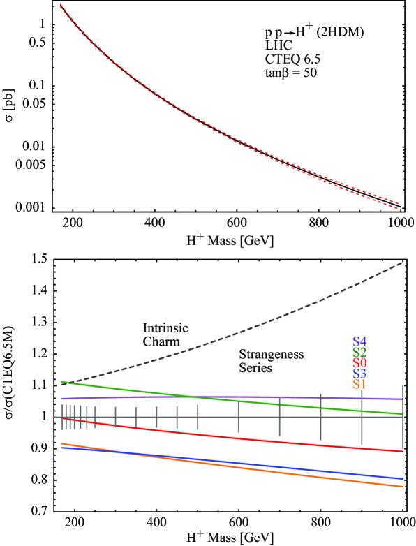
      (a)                                                                       (b)

Figure 7: The total cross section for charged Higgs boson production in 2HDM (top panel) and its fractional uncertainty (bottom panel) at (a) the Tevatron Run-2 and (b) the LHC.

The parton luminosity in the $c\,\bar{s}\to H^{+}$ process depends also on the behavior of the charm parton distribution. The CTEQ6.5Si series is generated under the conventional assumption that charm (anti)quarks are only perturbatively generated. Charm distributions of a non-perturbative origin—intrinsic charm (IC)—is both a theoretical possibility and phenomenologically allowed, as discussed recently in [17]. The existence of IC can significantly enhance the $H^{+}$ production cross section at the Tevatron. The dashed curve in the ratio plot of Fig. 7 represents the prediction obtained from a PDF set with a conventional strange input, but an intrinsic charm whose shape is given by the BHPS model [18, 17]. This dashed curve reflects the largest magnitude of the intrinsic charm contribution with $\langle x\rangle_{c+\bar{c}}=2.0\%$ allowed by the current hard scattering data [17]. Thus the enhancement in $H^{+}$ production due to intrinsic charm may be as large as a factor of 2–3, with important implications for the Tevatron experiments. A useful process to constrain the intrinsic charm contribution is the associated $Z\,c$ production, which will be discussed in another paper [12].

Figure 7(b) shows analogous plots for the $c\,\bar{s}\to H^{+}$ cross sections at the LHC. In this case, variations in the strangeness content may change the cross section in the shown range of Higgs boson masses by $\pm 10-20\%$. The intrinsic charm contributions may enhance the cross section by $10-50\%$. If $H^{+}$ is observed, the measurement of its production rate would provide clues about the underlying dynamics beyond the standard model. But for this test to be successful, uncertainties in strange and charm distributions must be reduced via independent measurements, such as dedicated studies of $W\,c$ and $Z\,c$ production.

6 Summary

We have systematically investigated the strangeness sector of the parton structure of the nucleon, using the latest theoretical tools and experimental input, within the framework of precision global QCD analysis. We find strong evidence that the strange quark distribution has a different shape compared to that of the isoscalar non-strange sea quark distribution.

We studied the range of possible magnitudes and shapes of the symmetric strange distribution function $s_{+}(x),$ using a 90% confidence level criterion. The range of allowed magnitude for the strange distribution, as measured by the average fractional momentum $\langle x\rangle_{s_{+}}$, is determined to be $0.018$–$0.040$. We present PDF sets that are representative of this range.

We find that the strangeness asymmetry function $s_{-}(x)$ is only loosely constrained. The range on the magnitude of this asymmetry, as measured by the momentum integral is determined to be $-0.001<\langle x\rangle_{s_{-}}<+0.005$, which is consistent with results in the existing literature.

We also discuss two sample applications of the PDFs presented in this study: the SM process $p\,p\mkern-11.0mu^{\scriptscriptstyle{(-)}}\to W^{+}+\,\bar{c}\,+X$ that can help further constrain the strange distributions; and the BSM process $p\,p\mkern-11.0mu^{\scriptscriptstyle{(-)}}\to H^{+}+X$, which depends sensitively on the strange and charm content of the nucleon.

The new PDFs discussed in this paper, CTEQ6.5Si, $i=0-4$, will be made available at the CTEQ web site (http://cteq.org/) and through the LHAPDF system
(http://hepforge.cedar.ac.uk/lhapdf/).

Acknowledgment

We thank Joey Huston for discussions and helpful comments. This work was supported in part by the U.S. National Science Foundation under awards PHY-0354838 and PHY-0555545; US Department of Energy, Division of High Energy Physics, Contract DE-AC02-06CH11357; and by the National Science Council of Taiwan under grant NSC-95-2112-M-133-001.

Appendix

There are currently some unresolved problems among fixed-target total inclusive neutrino and anti-neutrino scattering experiments on nuclear targets by CDHSW [19], CCFR [20, 21], NuTeV [22], and CHORUS [23], particularly in the large $x$ region. Comparisons of these experimental results can be found in Refs. [23] and [24]. A detailed study of these problems in the global analysis context, including effects of nuclear target corrections, has recently been performed in [25]. This open issue does not affect our study of the strange sector, since the strange distributions are insensitive to total inclusive cross sections, as demonstrated in Sections 3 and 4.

Specifically, the results presented in the main body of this paper were obtained by global analyses using fixed-target CC DIS data of CDHSW, CCFR, and CHORUS, which are mutually consistent. Separate fits were also done using the NuTeV total cross section data in place of these. Our findings can be summarized as follows: (i) these fits uniformly have much worse goodness-of-fit, to the point of beyond the 90% C.L. for many NC DIS data sets (BCDMS, H1, ZEUS); and (ii) if the resulting PDFs are taken at face value, all our conclusions about the (not so well-constrained) strange parton distributions remain valid, even as the better known $u,d,g$ distributions are shifted from previous determinations. Fig. 8 shows four typical $s_{+}(x)$ curves obtained using the NuTeV data set with different nuclear target corrections, compared to the CTEQ6.5S0,1,2 ones. We see that they are well within the range determined with our default data sets.

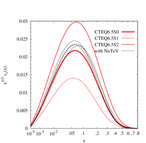
Figure 8: Typical symmetric strangeness sea $s_{+}(x)$ obtained using the NuTeV total inclusive data, represented by dotted lines, compared to CTEQ6.5S0,1,2 PDFs (solid curves).

References

- [1] W. K. Tung, AIP Conf. Proc. 753, 15 (2005) [Int. J. Mod. Phys. A 21, 620 (2006)] [hep-ph/0410139].
- [2] R. S. Thorne, “Parton distributions - DIS06,” hep-ph/0606307.
- [3] W. K. Tung, H. L. Lai, A. Belyaev, J. Pumplin, D. Stump and C.-P. Yuan, JHEP 0702, 053 (2007) [hep-ph/0611254].
- [4] M. Goncharov et al. [NuTeV Collaboration], Phys. Rev. D 64, 112006 (2001) [hep-ex/0102049].
- [5] E. Rondio et al. [NMC Collaboration], Nucl. Phys. A 553, 615C (1993).
- [6] D. A. Mason, to appear in the proceedings of 14th International Workshop on Deep Inelastic Scattering (DIS 2006), Tsukuba, Japan, 20-24 Apr 2006. (http://www-conf.kek.jp/dis06/doc/WG1/sf24-mason.pdf); and “Measurement of the strange - antistrange asymmetry at NLO in QCD from NuTeV dimuon data,” FERMILAB-THESIS-2006-01.
- [7] J. Pumplin, D. R. Stump and W. K. Tung, Phys. Rev. D 65, 014011 (2002) [hep-ph/0008191].
- [8] D. Stump et al., Phys. Rev. D 65, 014012 (2002) [hep-ph/0101051].
- [9] J. Pumplin, D. R. Stump, J. Huston, H. L. Lai, P. Nadolsky and W. K. Tung, JHEP 0207, 012 (2002) [hep-ph/0201195]; D. Stump, J. Huston, J. Pumplin, W. K. Tung, H. L. Lai, S. Kuhlmann and J. F. Owens, JHEP 0310, 046 (2003) [hep-ph/0303013].
- [10] F. Olness et al., Eur. Phys. J. C 40, 145 (2005) [hep-ph/0312323].
- [11] S.J. Brodsky, B.-Q. Ma, Phys. Lett. B381, 317 (1996); A.I. Signal and A.W. Thomas, Phys. Lett.B191, 205 (1987); F.G. Cao and A.I. Signal, Phys. Lett. B559, 229 (2003); M. Wakamatsu, Phys. Rev. D 67, 034005 (2003), and references therein.
- [12] P. Nadolsky, etal, “Implications of New Global QCD Analyses for Hadron Collider Physics”, in preparation.
- [13] W. T. Giele, S. Keller and E. Laenen, Nucl. Phys. Proc. Suppl. 51C, 255 (1996) [hep-ph/9606209].
- [14] P. B. Arnold and M. H. Reno, Nucl. Phys. B 319, 37 (1989) [Erratum-ibid. B 330, 284 (1990)].
- [15] H. E. Haber, G. Kane, S. Dawson, and J. F. Gunion, The Higgs Hunter’s Guide, Perseus Publishing, June 2000.
- [16] H. J. He and C.-P. Yuan, Phys. Rev. Lett. 83, 28 (1999) [hep-ph/9810367]; C. Balazs, H. J. He and C.-P. Yuan, Phys. Rev. D 60, 114001 (1999) [hep-ph/9812263].
- [17] J. Pumplin, H.L. Lai, and W.K. Tung, arXiv:hep-ph/0701220.
- [18] S. J. Brodsky, P. Hoyer, C. Peterson and N. Sakai, Phys. Lett. B 93, 451 (1980).
- [19] J. P. Berge et al., Z. Phys. C 49, 187 (1991).
- [20] CCFR Collaboration: U. K. Yang et al., Phys. Rev. Lett. 86 (2001) 2742 [hep-ex/0009041].
- [21] CCFR Collaboration: W. G. Seligman et al., Phys. Rev. Lett. 79 (1997) 1213 [hep-ex/970107].
- [22] M. Tzanov et al. [NuTeV Collaboration], Phys. Rev. D 74, 012008 (2006) [hep-ex/0509010].
- [23] G. Onengut et al. [CHORUS Collaboration], Phys. Lett. B 632, 65 (2006).
- [24] M. Tzanov, contribution to Proceedings of 13th International Workshop on Deep Inelastic Scattering; DIS 2005, Ed. Wesley H. Smith, Sridhara R. Dasu, AIP Conference Proceedings 792; and http://www-nutev.phyast.pitt.edu/results_2004/dis2005f.pdf
- [25] J.F. Owens, etal, arXiv:hep-ph/0702159.