Supersymmetric large $\tan\beta$ corrections to $\Delta M_{d,s}$ and $B_{d,s}\to\mu^{+}\mu^{-}$ revisited

Abstract

We point out that in the minimal supersymmetric standard model terms from the mixing of Higgs and Goldstone bosons which are connected to the renormalization of $\tan\beta$ via Slavnov-Taylor identities give rise to corrections that do not vanish in the limit where the supersymmetric particles are much heavier than the Higgs bosons. These additional contributions have important phenomenological implications as they can lead to potentially large supersymmetric effects in $\Delta M_{d}$ and to a significant increase of $\Delta M_{s}$ relative to the standard model prediction for a light pseudoscalar Higgs $A^{0}$. We calculate all the missing one-loop pieces and combine them with the known effective non-holomorphic terms to obtain improved predictions for the $B_{d,s}\text{--}\bar{B}_{d,s}$ mass differences $\Delta M_{d,s}$ and the branching ratios of $B_{d,s}\to\mu^{+}\mu^{-}$ in the large $\tan\beta$ regime of the minimal supersymmetric standard model with minimal-flavor-violation.

I Introduction

In minimal supersymmetric (SUSY) extensions of the standard model (SM) soft SUSY breaking terms are introduced that explicitly violate the underlying symmetry without spoiling the cancellation of quadratically divergent radiative corrections to the Higgs and other scalar masses. These soft terms must have positive mass dimension and the scale $M_{\rm SUSY}$ associated with them should be below a few TeV to naturally maintain the hierarchy between the electroweak scale $v$ and the Planck or any other very large energy scale. While theoretically little is known definitely about the origin and mechanism of the SUSY breaking itself, the soft mass terms will be measured and constrained as superpartners are detected. If SUSY is the solution to the hierarchy problem, then the Tevatron may, and the LHC will likely, find direct evidence for it. Meanwhile, the soft terms are also indirectly constrained by low-energy observables such as $\Delta M_{d,s}$, ${\cal B}(\bar{B}\to X_{s}\gamma)$, ${\cal B}(B_{d,s}\to\mu^{+}\mu^{-})$, ${\cal B}(B^{+}\to\tau^{+}\nu_{\tau})$, and $(g-2)_{\mu}$. From these measurements one can learn about the structure of SUSY breaking.

For large sparticle masses, i.e., $v/M_{\rm SUSY}\to 0$, the effects of SUSY degrees of freedom can be absorbed into the coupling constants of local operators in an effective theory that arises after decoupling the heavy particles. The corresponding low-energy theory is a two-Higgs-doublet model (THDM) of type II. In order for the THDM to be well-defined beyond tree-level, the effective couplings need to be calculated in the limit of unbroken $SU(2)\times U(1)$ symmetry. At the matching scale, some of the corrections to the effective couplings do not vanish for $M_{\rm SUSY}\to\infty$ if the Higgsino parameter $\mu$ is assumed to be of comparable size, i.e., $\mu={\cal O}(M_{\rm SUSY})$. In addition, some of the corrections can be enhanced by the ratio $\tan\beta=v_{u}/v_{d}$ of the vacuum expectation values (VEVs) $v_{d,u}$ of the two Higgs doublets $H_{d,u}$ that separately give masses to the down- and up-type fermions. As a result, they can be sizable, of order $\alpha_{s}\tan\beta\simeq 1$ for values of $\tan\beta\gg 1$, and need to be resummed if applicable.

In the minimal supersymmetric SM (MSSM) with minimal-flavor-violation (MFV), four different types of large $\tan\beta$ contributions that affect the interactions between Higgs bosons and SM fermions have been identified: (i) corrections to the vertices between a Higgs boson and down-type fermions Hall:1993gn , which are interpreted as corrections to the Yukawa couplings $y_{d}$ and resummed Carena:1999py , (ii) similar corrections to the vertices between a Higgs boson and up-type fermions ltbup which are not resummed, (iii) corrections to the Cabibbo-Kobayashi-Maskawa (CKM) matrix elements Blazek:1995nv , and (iv) flavor-changing neutral Higgs vertex corrections Babu:1999hn , which do not appear at tree-level.

The purpose of this article is it to point out that there are additional terms from mixing of Higgs and Goldstone bosons UN which are connected to the renormalization of $\tan\beta$. These new contributions have important phenomenological implications as they can lead to potentially large SUSY effects in $\Delta M_{d}$ and to a significant increase of $\Delta M_{s}$ relative to the SM prediction in a certain region of the allowed parameter space. Both findings go against common lore BCRS ; Isidori:2001fv ; D'Ambrosio:2002ex ; Carena:2006ai ; Blanke:2006ig ; recent , but they are an unavoidable consequence of the analysis presented here.

This article is organized as follows. In the next section we derive the $\tan\beta$ enhanced corrections to the effective Higgs interactions with quarks of the third generation, including all terms that arise from the one-loop mixing between eigenstates of the two Higgs doublets. Analytic formulas for the neutral Higgs contributions to $\Delta M_{d,s}$ and ${\cal B}(B_{d,s}\to\mu^{+}\mu^{-})$ are presented in Sec. III. Sec. IV contains a numerical analysis of $\Delta M_{d,s}$ in the MFV MSSM with large $\tan\beta$ taking into account all relevant constraints from flavor and collider physics. Concluding remarks are given in Sec. V.

II Effective theory

Beyond leading order, the physical Higgs fields $A^{0}$ and $H^{\pm}$ can mix with the longitudinal components of the gauge bosons fields $Z^{0}$ and $W^{\pm}$ through loop corrections. This mixing has to be removed for on-shell momenta by suitable rotations of the fields. Due to the connection between the longitudinal gauge bosons and the Goldstone bosons $G^{0}$ and $G^{\pm}$, this procedure also implies field renormalization for the mixing between Higgs and Goldstone bosons. The relation between the terms with gauge and Goldstone bosons is given by Slavnov-Taylor identities (STIs), derived from the invariance of two-point functions under Becchi-Rouet-Stora-Tyutin transformations. In our case the relevant STIs are given to one-loop order by

$$0=k^{\mu}\hat{\Sigma}_{\mu}^{VS}(k)+\widetilde{M}_{V}\hat{\Sigma}^{S^{\prime}S}(k^{2})+\ldots\,,$$ (1)

where $\{V,S,S^{\prime},\widetilde{M}_{V}\}=\{Z^{0},A^{0},G^{0},iM_{Z}\}$, $\{W^{\pm},H^{\mp},$ $G^{\pm},\pm M_{W}\}$, and hatted quantities denote amputated and renormalized mixing self-energies. The ellipses stand for terms that vanish in the limit $k^{2}\to M_{S}^{2}$ which are irrelevant for the further discussion.

In the renormalized mixing self-energies, besides the field renormalization counterterms $\delta Z^{S^{\prime}S}$, the contributions from the tadpole renormalization, $\delta t_{d,u}$, and from the renormalization of the VEVs, $\delta Z_{d,u}$, need to be included. The tadpole counterterms are fixed by the requirement that the properly minimized scalar potential should have no finite tadpole terms, $\hat{t}_{d,u}=t_{d,u}+\delta t_{d,u}=0$. The renormalization of the VEVs, $\hat{v}_{d,u}=(1+\delta Z_{d,u})v_{d,u}$, translates into the renormalization of the gauge boson masses and $\tan\beta$, $\delta\tan\beta=(\delta Z_{u}-\delta Z_{d})\tan\beta$. Here quantities without hat denote unrenormalized contributions.

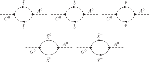
Figure 1: Diagrams in the MSSM that lead to non-decoupling corrections to the $G^{0}A^{0}$ mixing self-energy. See text for details.

Decomposing the $VS$ mixing self-energy via $\hat{\Sigma}_{\mu}^{VS}(k)=k_{\mu}\hat{\Sigma}^{VS}(k^{2})$ and using the above conventions the renormalized self-energies can be written as

$$\begin{split}\hat{\Sigma}^{VS}(k^{2})&=\Sigma^{VS}(k^{2})-\widetilde{M}_{V}\frac{1}{2}\delta Z^{S^{\prime}S}+\widetilde{M}_{V}c_{\beta}^{2}\,\delta t_{\beta}\,,\\ \hat{\Sigma}^{S^{\prime}S}(k^{2})&=\Sigma^{S^{\prime}S}(k^{2})+\frac{1}{2}k^{2}\delta Z^{S^{\prime}S}-M_{S}^{2}c_{\beta}^{2}\,\delta t_{\beta}\\ &+\frac{g}{2M_{W}}\left(c_{\beta-\alpha}\,\delta t_{h^{0}}-s_{\beta-\alpha}\,\delta t_{H^{0}}\right)+\ldots\,,\end{split}$$ (2)

where again terms that vanish on-shell have been omitted. Furthermore the abbreviations $s_{\beta}=\sin\beta$, $c_{\beta}=\cos\beta$, $t_{\beta}=\tan\beta$, etc. have been used and the tadpoles of the $H_{d,u}$ fields expressed in terms of those of the Higgs mass eigenstates $h^{0}$ and $H^{0}$.

Requiring now that the mixing between longitudinal gauge and Higgs bosons vanishes when the Higgs boson momentum is on-shell, $\hat{\Sigma}^{VS}(M_{S}^{2})=0$, one obtains for the field renormalization counterterms

$$\begin{split}\delta Z^{S^{\prime}S}&=\frac{2}{\widetilde{M}_{V}}\Sigma^{VS}(M_{S}^{2})+2c_{\beta}^{2}\,\delta t_{\beta}\\ &=-\frac{2}{M_{S}^{2}}\Sigma^{S^{\prime}S}(M_{S}^{2})+2c_{\beta}^{2}\,\delta t_{\beta}\\ &-\frac{g}{M_{S}^{2}M_{W}}\left(c_{\beta-\alpha}\,\delta t_{h^{0}}-s_{\beta-\alpha}\,\delta t_{H^{0}}\right)\,.\end{split}$$ (3)

The presence of $\delta t_{\beta}$ in the above equalities illustrates that beyond tree-level a definition of $\tan\beta$ is needed, which in turn controls the extent of mixing between Higgs and Goldstone boson fields.

Several prescriptions for the renormalization of $\tan\beta$ have been studied in the literature, but from a careful analysis Freitas:2002um it was found that in order to avoid large higher order corrections, the best scheme is to use $\overline{\rm DR}$ renormalization for $\tan\beta$, which is manifestly process-independent to all orders and gauge-independent at the one-loop level within the class of $R_{\xi}$ gauges. If only the leading contributions for large $\tan\beta$ are retained, the counterterm $\delta\tan\beta$ is thus identical to zero.

In the limit $\tan\beta\gg 1$, the leading contribution to the field renormalization counterterms involving SUSY loops are of zeroth order in $\tan\beta$. The Feynman diagrams that lead to the non-decoupling corrections to the $G^{0}A^{0}$ mixing self-energy are shown in Fig. 1. Calculating these, the corresponding $G^{\pm}H^{\mp}$ diagrams, and the tadpole counterterms in the limit of unbroken $SU(2)\times U(1)$ symmetry we find

$$\frac{1}{2}\delta Z^{G^{0}A^{0}}=\frac{1}{2}\delta Z^{G^{\pm}H^{\mp}}=\epsilon_{\rm GP}\,,$$ (4)

where

$$\epsilon_{\rm GP} =-\frac{\mu}{32\pi^{2}}\Bigg{[}3y_{t}^{2}\frac{A_{t}}{m_{\tilde{t}_{R}}^{2}}H_{1}(x_{\tilde{t}})+3y_{b}^{2}\frac{A_{b}}{m_{\tilde{b}_{R}}^{2}}H_{1}(x_{\tilde{b}})$$ (5)

$$+y_{\tau}^{2}\frac{A_{\tau}}{m_{\tilde{\tau}_{R}}^{2}}H_{1}(x_{\tilde{\tau}})+g^{\prime 2}\frac{M_{1}}{\mu^{2}}H_{1}(x_{1})+3g^{2}\frac{M_{2}}{\mu^{2}}H_{1}(x_{2})\Bigg{]},$$

and

$$H_{1}(x)=\frac{x+1}{(x-1)^{2}}-\frac{2x}{(x-1)^{3}}\ln x\,.$$ (6)

The variables $x_{\tilde{f}}=m^{2}_{\tilde{f}_{L}}/m^{2}_{\tilde{f}_{R}}$ and $x_{i}=M^{2}_{i}/\mu^{2}$ denote the ratios of the left- and right-handed sfermion masses and the soft SUSY breaking masses $M_{1,2}$ and the Higgsino parameter $\mu$ squared. We assume $CP$ conservation, so all soft SUSY breaking terms are real.

For sizable values of the tri-linear soft SUSY breaking couplings $A_{t,b}$ the correction $\epsilon_{\rm GP}$ is dominated by the stop and sbottom contributions, which are proportional to the square of the Yukawa couplings $y_{t,b}$. The stau and bino corrections are numerically insignificant. Assuming the values of $|\mu|$, $|A_{t}|$, $m_{\tilde{t}_{L}}$, and $m_{\tilde{t}_{R}}$ to be degenerate and keeping only the stop contribution one finds $\epsilon_{\rm GP}\simeq-{\rm sign}(\mu A_{t})/(32\pi^{2})\simeq-3\times 10^{-3}\,{\rm sign}(\mu A_{t})$, while $|\epsilon_{\rm GP}|$ can reach $\simeq 10^{-2}$ for $\tan\beta\gg 1$ and natural choices of sfermion masses and soft SUSY breaking parameters in the ${\rm TeV}$ range.

The corrections (4) as such are not $\tan\beta$ enhanced. However, since they describe the mixing between eigenstates of the two Higgs doublets, they replace $\tan\beta$ suppressed Higgs-fermion couplings with the non-suppressed Goldstone-fermion couplings. The $\tan\beta$ suppression at tree-level is therefore effectively lifted at the one-loop level. Obviously, this can only occur at the next-to-leading order (NLO) and there are no resummable enhanced $\tan\beta$ corrections beyond that order.

The term $\epsilon_{\rm GP}$ can also be derived from the STIs of the $CP$-even neutral Higgs sector. In this case one demands un-mixing of the on-shell Higgs bosons at loop level, and needs to take into account the renormalization of other parameters of the Higgs potential in the broken phase, such as the on-shell renormalization of the gauge boson masses. We find

$$\frac{M_{h^{0}}^{2}-M_{H^{0}}^{2}}{2M_{H^{0}}^{2}}\delta Z^{h^{0}H^{0}}=\frac{M_{H^{0}}^{2}-M_{h^{0}}^{2}}{2M_{h^{0}}^{2}}\delta Z^{H^{0}h^{0}}=\epsilon_{\rm GP}\,.$$ (7)

As a result, the mixing of $h^{0}$ and $H^{0}$ receives particularly large contributions from $\epsilon_{\rm GP}$ if the difference between the masses $M_{h^{0}}$ and $M_{H^{0}}$ is small.

The term $\epsilon_{\rm GP}$ essentially describes the mixing between the two Higgs doublets at one loop. Therefore the resulting contributions are universal for the different $CP$ and charge scalar eigenstates, up to the different mixing in the $CP$-even neutral sector, which is described here through the Higgs masses in Eq. (7).

The diagonalization of the Higgs mass matrix necessarily induces diagonal and off-diagonal couplings of the neutral and charged scalar to the quark fields. In the basis of neutral and charged Higgs mass eigenstates the large $\tan\beta$ corrections to the effective Higgs interactions with quarks of the third generation can be cast into the following form

$${\cal L}_{\rm eff} =G_{F}^{1/2}2^{1/4}\Bigg{\{}\frac{\overline{m}_{b}t_{\beta}}{1+\tilde{\epsilon}_{3}\,t_{\beta}}\Bigg{[}i\bar{b}_{{\scalebox{0.6}{$L$}}}b_{{\scalebox{0.6}{$R$}}}A^{0}+\bigg{(}\frac{s_{\alpha}}{s_{\beta}}-\frac{c_{\alpha}}{s_{\beta}}\,\tilde{\epsilon}_{3}+\frac{M_{h^{0}}^{2}}{M_{H^{0}}^{2}-M_{h^{0}}^{2}}\frac{c_{\alpha}}{s_{\beta}}\,\epsilon_{\rm GP}\bigg{)}\bar{b}_{{\scalebox{0.6}{$L$}}}b_{{\scalebox{0.6}{$R$}}}h^{0}$$

$$\hskip 100.00015pt-\bigg{(}\frac{c_{\alpha}}{s_{\beta}}+\frac{s_{\alpha}}{s_{\beta}}\,\tilde{\epsilon}_{3}\bigg{)}\bar{b}_{{\scalebox{0.6}{$L$}}}b_{{\scalebox{0.6}{$R$}}}H^{0}+\sqrt{2}V_{tb}^{\rm eff}\,\bar{t}_{{\scalebox{0.6}{$L$}}}b_{{\scalebox{0.6}{$R$}}}H^{+}\Bigg{]}$$

$$+\frac{\epsilon_{Y}y_{t}^{2}t_{\beta}^{2}}{(1+\tilde{\epsilon}_{3}\,t_{\beta})(1+\epsilon_{0}\,t_{\beta})}\Bigg{[}i\left(V_{tb}^{{\rm eff}\ast}V_{td^{i}}^{\rm eff}\,\overline{m}_{b}\,\bar{b}_{{\scalebox{0.6}{$R$}}}d^{i}_{{\scalebox{0.6}{$L$}}}A^{0}-V_{td^{i}}^{{\rm eff}\ast}V_{tb}^{\rm eff}\,\overline{m}_{d_{i}}\,\bar{b}_{{\scalebox{0.6}{$L$}}}d^{i}_{{\scalebox{0.6}{$R$}}}A^{0}\right)$$

$$\hskip 100.00015pt-\bigg{(}\frac{c_{\alpha-\beta}}{s_{\beta}^{2}}+\frac{M_{h^{0}}^{2}}{M_{H^{0}}^{2}-M_{h^{0}}^{2}}\frac{c_{\alpha}}{s_{\beta}}\,\epsilon_{\rm GP}\bigg{)}\left(V_{tb}^{{\rm eff}\ast}V_{td^{i}}^{\rm eff}\,\overline{m}_{b}\,\bar{b}_{{\scalebox{0.6}{$R$}}}d^{i}_{{\scalebox{0.6}{$L$}}}h^{0}+V_{td^{i}}^{{\rm eff}\ast}V_{tb}^{\rm eff}\,\overline{m}_{d_{i}}\,\bar{b}_{{\scalebox{0.6}{$L$}}}d^{i}_{{\scalebox{0.6}{$R$}}}h^{0}\right)$$

$$\hskip 100.00015pt-\frac{s_{\alpha-\beta}}{s_{\beta}^{2}}\left(V_{tb}^{{\rm eff}\ast}V_{td^{i}}^{\rm eff}\,\overline{m}_{b}\,\bar{b}_{{\scalebox{0.6}{$R$}}}d^{i}_{{\scalebox{0.6}{$L$}}}H^{0}+V_{td^{i}}^{{\rm eff}\ast}V_{tb}^{\rm eff}\,\overline{m}_{d_{i}}\,\bar{b}_{{\scalebox{0.6}{$L$}}}d^{i}_{{\scalebox{0.6}{$R$}}}H^{0}\right)\Bigg{]}$$

$$+\overline{m}_{t}\Bigg{[}\big{(}t_{\beta}^{-1}-\epsilon_{0}^{\prime}-\epsilon_{Y}^{\prime}y_{b}^{2}+\epsilon_{\rm GP}\big{)}\big{(}i\bar{t}_{{\scalebox{0.6}{$L$}}}t_{{\scalebox{0.6}{$R$}}}A^{0}+\sqrt{2}V_{tb}^{\rm eff}\,\bar{t}_{{\scalebox{0.6}{$R$}}}b_{{\scalebox{0.6}{$L$}}}H^{+}\big{)}-\frac{c_{\alpha}}{s_{\beta}}\bar{t}_{{\scalebox{0.6}{$L$}}}t_{{\scalebox{0.6}{$R$}}}h^{0}-\frac{s_{\alpha}}{s_{\beta}}\bar{t}_{{\scalebox{0.6}{$L$}}}t_{{\scalebox{0.6}{$R$}}}H^{0}\Bigg{]}\Bigg{\}}+{\rm h.c.}\,,$$

for $d^{i}=d,s$. Here $G_{F}$ denotes the Fermi constant, $V_{ij}^{\rm eff}$ are the physical CKM matrix elements, and $\overline{m}_{f}$ are running $\overline{\rm MS}$ masses evaluated at a scale of order $m_{t}$, which are connected to the Yukawa couplings through $y^{2}_{t}=2\sqrt{2}G_{F}\overline{m}_{t}^{2}$ and $y^{2}_{b}=2\sqrt{2}G_{F}\overline{m}_{b}^{2}t_{\beta}^{2}/(1+\tilde{\epsilon}_{3}\,t_{\beta})^{2}$. The subscripts $L$ and $R$ indicate the chirality of the quark fields involved in the interaction.

As the field renormalization counterterms $\delta Z^{S^{\prime}S}$ in Eqs. (4) and (7) cancel the momentum-independent part of the mixing self-energies $\Sigma^{S^{\prime}S}(k^{2})$, dimension four operators related to the mixing of the scalar fields $\{S,S^{\prime}\}=\{A^{0},G^{0}\}$, $\{H^{\mp},G^{\pm}\}$, $\{h^{0},H^{0}\}$, and $\{H^{0},h^{0}\}$ are removed from the effective theory. Alternatively, if the vanishing of the $S^{\prime}S$ mixing in the full theory is not enforced by suitable renormalization conditions, then diagrams with insertions of dimension four operators that mix the scalar fields $S^{\prime}$ and $S$ will contribute on the effective side. If implemented correctly, the two strategies lead naturally to identical results for physical observables.

The epsilon parameters $\tilde{\epsilon}_{3}$, $\epsilon_{0}$, $\epsilon_{Y}$, $\epsilon_{0}^{\prime}$, and $\epsilon_{Y}^{\prime}$ are defined as in BCRS . In our numerical analysis we employ them in the limit of unbroken $SU(2)\times U(1)$ and include all effects proportional to the $SU(2)$ couplings $g$ and $g^{\prime}$ squared. The corresponding analytic expressions read

$$\tilde{\epsilon}_{3} =\epsilon_{0}+\epsilon_{Y}y_{t}^{2}\,,$$ (9)

$$\epsilon_{0} =-\frac{2\alpha_{s}}{3\pi}\frac{\mu}{M_{\tilde{g}}}H_{2}(u_{\tilde{t}_{L}},u_{\tilde{b}_{R}})$$

$$+\frac{1}{16\pi^{2}}\bigg{[}\frac{g^{\prime 2}}{6}\frac{M_{1}}{\mu}\big{(}H_{2}(v_{\tilde{t}_{L}},x_{1})+2H_{2}(v_{\tilde{b}_{R}},x_{1})\big{)}$$ (10)

$$\hskip 25.00003pt+\frac{g^{\prime 2}}{9}\frac{\mu}{M_{1}}H_{2}(w_{\tilde{t}_{L}},w_{\tilde{b}_{R}})+\frac{g^{2}}{2}\frac{M_{2}}{\mu}H_{2}(v_{\tilde{t}_{L}},x_{2})\bigg{]},$$

$$\epsilon_{Y} =\frac{-1}{16\pi^{2}}\bigg{[}\frac{A_{t}}{\mu}H_{2}(v_{\tilde{t}_{L}},v_{\tilde{t}_{R}})-\frac{g^{2}}{y_{t}^{2}}\frac{M_{2}}{\mu}H_{2}(v_{\tilde{t}_{L}},x_{2})\bigg{]},$$ (11)

$$\epsilon_{0}^{\prime} =-\frac{2\alpha_{s}}{3\pi}\frac{\mu}{M_{\tilde{g}}}H_{2}(u_{\tilde{t}_{L}},u_{\tilde{t}_{R}})$$

$$-\frac{1}{16\pi^{2}}\bigg{[}\frac{g^{\prime 2}}{6}\frac{M_{1}}{\mu}\big{(}H_{2}(v_{\tilde{t}_{L}},x_{1})-4H_{2}(v_{\tilde{t}_{R}},x_{1})\big{)}$$ (12)

$$\hskip 25.00003pt+\frac{2g^{\prime 2}}{9}\frac{\mu}{M_{1}}H_{2}(w_{\tilde{t}_{L}},w_{\tilde{t}_{R}})-\frac{g^{2}}{2}\frac{M_{2}}{\mu}H_{2}(v_{\tilde{t}_{L}},x_{2})\bigg{]},$$

$$\epsilon_{Y}^{\prime} =\frac{-1}{16\pi^{2}}\bigg{[}\frac{A_{b}}{\mu}H_{2}(v_{\tilde{t}_{L}},v_{\tilde{b}_{R}})-\frac{g^{2}}{y_{b}^{2}}\frac{M_{2}}{\mu}H_{2}(v_{\tilde{t}_{L}},x_{2})\bigg{]}.$$ (13)

Here $u_{\tilde{q}}=m^{2}_{\tilde{q}}/M_{\tilde{g}}^{2}$, $v_{\tilde{f}}=m^{2}_{\tilde{f}}/\mu^{2}$, $w_{\tilde{f}}=m^{2}_{\tilde{f}}/M_{1}^{2}$, and

$$H_{2}(x,y)=\frac{x\ln x}{(1-x)(x-y)}+\frac{y\ln y}{(1-y)(y-x)}\,.$$ (14)

Our analytic results for $\tilde{\epsilon}_{3}$, $\epsilon_{0}$, $\epsilon_{Y}$, $\epsilon_{0}^{\prime}$, and $\epsilon_{Y}^{\prime}$ have been obtained in the approximation $V_{ud}\simeq V_{cs}\simeq V_{tb}\simeq 1$. They agree with the corresponding expressions in Hall:1993gn ; Carena:1999py ; Blazek:1995nv ; Babu:1999hn ; ltbup ; BCRS ; Isidori:2001fv ; D'Ambrosio:2002ex for $g=g^{\prime}=0$.

III Double penguin contributions to $\Delta M_{d,s}$ and ${\cal B}(B_{d,s}\to\mu^{+}\mu^{-})$

The unique role of neutral Higgs double penguin (DP) contributions to $\Delta M_{d,s}$ and ${\cal B}(B_{d,s}\to\mu^{+}\mu^{-})$ has been extensively discussed in the literature BCRS ; Isidori:2001fv ; D'Ambrosio:2002ex ; Carena:2006ai ; recent ; other . In the following, we extend these analyses by incorporating the effects due to the new term $\epsilon_{\rm GP}$. This allows us to obtain improved predictions for $\Delta M_{d,s}$ and ${\cal B}(B_{d,s}\to\mu^{+}\mu^{-})$ in the large $\tan\beta$ regime of the MFV MSSM based on the $SU(2)\times U(1)$ symmetry limit.

Predicting the $B_{d,s}\text{--}\bar{B}_{d,s}$ mass differences involves integrating out heavy degrees of freedom at a scale of order $m_{t}$ by matching on to the effective Hamiltonian

$${\cal H}_{\rm eff}^{\Delta B=2}=\frac{G_{F}^{2}M_{W}^{2}}{16\pi^{2}}(V_{tb}^{{\rm eff}\ast}V_{td^{i}}^{\rm eff})^{2}\sum_{j}C_{j}Q_{j}+{\rm h.c.}$$ (15)

In the MFV MSSM with large $\tan\beta$ the numerically dominant contributions to $\Delta M_{d,s}$ are induced by the two effective operators

$$Q_{2}^{\rm LR}=(\bar{b}_{{\scalebox{0.6}{$R$}}}d^{i}_{{\scalebox{0.6}{$L$}}})(\bar{b}_{{\scalebox{0.6}{$L$}}}d^{i}_{{\scalebox{0.6}{$R$}}})\,,\hskip 7.11317ptQ_{1}^{\rm SLL}=(\bar{b}_{{\scalebox{0.6}{$R$}}}d^{i}_{{\scalebox{0.6}{$L$}}})(\bar{b}_{{\scalebox{0.6}{$R$}}}d^{i}_{{\scalebox{0.6}{$L$}}})\,.$$ (16)

Combining the flavor-changing neutral Higgs couplings of Eq. (II) we find that the initial conditions of the corresponding Wilson coefficients are given by

$$C_{2}^{\rm LR} =-\frac{G_{F}\overline{m}_{b}\overline{m}_{d_{i}}\overline{m}_{t}^{4}}{\sqrt{2}\pi^{2}M_{W}^{2}}\frac{(16\pi^{2})^{2}\,t_{\beta}^{4}\,\epsilon_{Y}^{2}\,\cal{F}^{+}}{(1+\tilde{\epsilon}_{3}\,t_{\beta})^{2}(1+\epsilon_{0}\,t_{\beta})^{2}}\,,\hskip 5.69054pt$$ (17)

$$C_{1}^{\rm SLL} =-\frac{G_{F}\overline{m}_{b}^{2}\overline{m}_{t}^{4}}{2\sqrt{2}\pi^{2}M_{W}^{2}}\frac{(16\pi^{2})^{2}\,t_{\beta}^{4}\,\epsilon_{Y}^{2}\,\cal{F}^{-}}{(1+\tilde{\epsilon}_{3}\,t_{\beta})^{2}(1+\epsilon_{0}\,t_{\beta})^{2}}\,,$$

where

$$\begin{split}{\cal F}^{\pm}&=\frac{s_{\alpha-\beta}^{2}}{M_{H^{0}}^{2}}+\frac{c_{\alpha-\beta}^{2}}{M_{h^{0}}^{2}}\pm\frac{1}{M_{A^{0}}^{2}}\\ &+\frac{c_{\alpha}\,(2c_{\alpha-\beta}+c_{\alpha}\,\delta_{\rm GP})\,\delta_{\rm GP}}{M_{h^{0}}^{2}}\,,\end{split}$$ (18)

and

$$\delta_{\rm GP}=\frac{M_{h^{0}}^{2}}{M_{H^{0}}^{2}-M_{h^{0}}^{2}}\,\epsilon_{\rm GP}\,.$$ (19)

Here we have used the approximations $\sin\beta\simeq 1$ and $\cos\beta\simeq 0$ valid for $\tan\beta\gg 1$. The same relations are employed in the following whenever it is justified. The first line of Eq. (18) resembles the result derived first by the authors of BCRS , while the second one represents the new contribution to the factors $\cal{F}^{\pm}$ due to $\epsilon_{\rm GP}$.

Using $\Delta M_{d,s}=|\langle B_{d,s}|{\cal H}_{\rm eff}^{\Delta B=2}|\bar{B}_{d,s}\rangle|/M_{B_{d,s}}$ one obtains from Eq. (15) the DP contribution to the $B_{d,s}\text{--}\bar{B}_{d,s}$ mass differences. To an excellent approximation one has

$$\begin{split}\Delta M_{d^{i}}^{\rm DP}&=\frac{G_{F}^{2}M_{W}^{2}}{24\pi^{2}}M_{B_{d^{i}}}f_{B_{d^{i}}}^{2}\times\\ &|V_{tb}^{{\rm eff}\ast}V_{td^{i}}^{\rm eff}|^{2}\left(P_{2}^{\rm LR}C_{2}^{\rm LR}+P_{1}^{\rm SLL}C_{1}^{\rm SLL}\right)\,,\end{split}$$ (20)

where the factors $P_{2}^{\rm LR}=2.56$ and $P_{1}^{\rm SLL}=-1.06$ condense renormalization-group-improved NLO QCD corrections Buras:2000if and the relevant matrix elements Becirevic:2001xt . In our numerical analysis we employ the unquenched staggered three flavor results $f_{B_{d}}=216(22)\hskip 0.7113pt{\rm MeV}$ Gray:2005ad and $f_{B_{s}}=260(29)\hskip 0.7113pt{\rm MeV}$ Wingate:2003gm for the $B_{d,s}$-meson decay constants obtained by the HPQCD Collaboration, while we take $|V_{tb}^{{\rm eff}\ast}V_{td}^{\rm eff}|=86(14)\times 10^{-4}$, $|V_{tb}^{{\rm eff}\ast}V_{ts}^{\rm eff}|=41.3(7)\times 10^{-3}$ Ball:2006xx , $M_{B_{d}}=5.2793\hskip 0.7113pt{\rm GeV}$, and $M_{B_{s}}=5.3696\hskip 0.7113pt{\rm GeV}$ Yao:2006px .

In the case of the rare decays $B_{d,s}\to\mu^{+}\mu^{-}$, the effective Hamiltonian that arises after removing all heavy particles as active degrees of freedom is given by

$${\cal H}_{\rm eff}^{\Delta B=1}=-\frac{G_{F}}{\sqrt{2}}\frac{\alpha_{\rm em}}{\pi s^{2}_{W}}V_{tb}^{{\rm eff}\ast}V_{td^{i}}^{\rm eff}\sum_{j}C_{j}Q_{j}+{\rm h.c.}\,,$$ (21)

where the electromagnetic coupling $\alpha_{\rm em}$ and the weak mixing angle $s_{W}$ are naturally evaluated at the electroweak scale Bobeth:2003at .

In the large $\tan\beta$ regime of the MFV MSSM only two effective operators can have a sizable impact on $B_{d,s}\to\mu^{+}\mu^{-}$, namely

$$Q_{S}=m_{b}(\bar{b}_{{\scalebox{0.6}{$R$}}}d^{i}_{{\scalebox{0.6}{$L$}}})(\bar{\mu}\mu)\,,\hskip 7.11317ptQ_{P}=m_{d^{i}}(\bar{b}_{{\scalebox{0.6}{$L$}}}d^{i}_{{\scalebox{0.6}{$R$}}})(\bar{\mu}\gamma_{5}\mu)\,.$$ (22)

The same flavor-changing Higgs vertices that generate the dominant contribution to $\Delta M_{d,s}$ induce enhanced $\tan\beta$ corrections to the Wilson coefficients of the semileptonic operators $Q_{S}$ and $Q_{P}$. The effective couplings of Eq. (II) lead to the following matching conditions

$$\begin{split}&C_{S}=\frac{m_{\mu}\overline{m}_{t}^{2}}{4M_{W}^{2}}\frac{16\pi^{2}\,t_{\beta}^{3}\,\epsilon_{Y}}{(1+\tilde{\epsilon}_{3}\,t_{\beta})(1+\epsilon_{0}\,t_{\beta})}\Bigg{[}\frac{c_{\alpha}s_{\alpha-\beta}}{M_{H^{0}}^{2}}\\ &-\frac{s_{\alpha}c_{\alpha-\beta}}{M_{h^{0}}^{2}}-\frac{c_{\alpha}\,(c_{\alpha-\beta}+s_{\alpha}+c_{\alpha}\,\delta_{\rm GP})\,\delta_{\rm GP}}{M_{h^{0}}^{2}}\Bigg{]}\,,\\ &C_{P}=-\frac{m_{\mu}\overline{m}_{t}^{2}}{4M_{W}^{2}}\frac{16\pi^{2}\,t_{\beta}^{3}\,\epsilon_{Y}}{(1+\tilde{\epsilon}_{3}\,t_{\beta})(1+\epsilon_{0}\,t_{\beta})}\frac{1}{M_{A^{0}}^{2}}\,,\end{split}$$ (23)

where $m_{\mu}=105.66\hskip 1.42262pt{\rm MeV}$ Yao:2006px . While $C_{P}$ remains unchanged with respect to the analytic expression first presented in BCRS , $C_{S}$ picks up an additional contribution due to $\epsilon_{\rm GP}$ given by the second term in the second line of Eq. (23).

The DP contribution to the branching ratios of $B_{d,s}\to\mu^{+}\mu^{-}$ can be expressed to a very good approximation in terms of the initial conditions $C_{S}$ and $C_{P}$ as

$$\begin{split}{\cal B}(B_{d^{i}}\to\mu^{+}\mu^{-})^{\rm DP}&=\frac{G_{F}^{2}\alpha_{\rm em}M_{B_{d^{i}}}^{5}f_{B_{d^{i}}}^{2}\tau_{B_{d^{i}}}}{64\pi^{3}}\times\\ &|V_{tb}^{{\rm eff}\ast}V_{td^{i}}^{\rm eff}|^{2}\left(|C_{S}|^{2}+|C_{P}|^{2}\right)\,,\end{split}$$ (24)

where the $B_{d,s}$-meson lifetimes are taken to be $\tau_{B_{d}}=1.527\hskip 0.7113pt{\rm ps}$ and $\tau_{B_{s}}=1.454\hskip 0.7113pt{\rm ps}$ Barberio:2006bi .

IV Numerical analysis

We are now in the position to analyze the impact of the correction $\epsilon_{\rm GP}$ on the prediction of $\Delta M_{d,s}$ in the MFV MSSM with large $\tan\beta$, taking into account the constraints from the low-energy observables $\Delta M_{K}$, $|\epsilon_{K}|$, ${\cal B}(\bar{B}\to X_{s}\gamma)$, ${\cal B}(\bar{B}\to X_{s}l^{+}l^{-})$, ${\cal B}(B_{d,s}\to\mu^{+}\mu^{-})$, and ${\cal B}(B^{+}\to\tau^{+}\nu_{\tau})$, as well as the limit on the lightest Higgs boson mass $M_{h^{0}}$. In the calculation of the flavor physics observables all relevant contributions stemming from $A^{0}$, $h^{0}$, $H^{0}$, $H^{\pm}$, and $\tilde{\chi}^{\pm}$ exchange are taken into account. More precisely, in the case of $\Delta M_{K}$ and $|\epsilon_{K}|$ we rely on the formulas given in Carena:2006ai , while our calculation of ${\cal B}(\bar{B}\to X_{s}\gamma)$ includes all $\tan\beta$ enhanced charged Higgs and chargino corrections ltbup as well as the DP contribution D'Ambrosio:2002ex . In the case of $\Delta M_{s}$ we combine the neutral Higgs effects with the $\tan\beta$ resummed terms from charged Higgs box diagrams BCRS ; Isidori:2001fv , while for ${\cal B}(B^{+}\to\tau^{+}\nu_{\tau})$ we employ the formula first derived in Akeroyd:2003zr . In all cases we supplement the existing expressions with the corrections stemming from the new term $\epsilon_{\rm GP}$ and use the complete formulas Eqs. (9) to (13) for $\tilde{\epsilon}_{3}$, $\epsilon_{0}$, $\epsilon_{Y}$, $\epsilon_{0}^{\prime}$, and $\epsilon_{Y}^{\prime}$.

Another important difference with respect to the preceding analyses BCRS ; Isidori:2001fv ; D'Ambrosio:2002ex ; Carena:2006ai ; recent is the fact that we do not evaluate the mixing angle $\alpha$ and the masses $M_{h^{0}}$ and $M_{H^{0}}$ appearing in Eqs. (18) and (23) at tree-level, but include the dominant one-loop corrections mhsusy , which are essential to obtain $M_{h^{0}}>M_{Z}$. While the inclusion of these higher order corrections turns out to have a minor impact on $\Delta M_{s}$ and $B_{d,s}\to\mu^{+}\mu^{-}$, we find that they have a profound effect on $\Delta M_{d}$, as they invalidate the common assumption BCRS ; Isidori:2001fv ; D'Ambrosio:2002ex ; Carena:2006ai ; recent that $C_{1}^{\rm SLL}$ gives only a negligible contribution to the $B_{d}\text{--}\bar{B}_{d}$ mass difference.

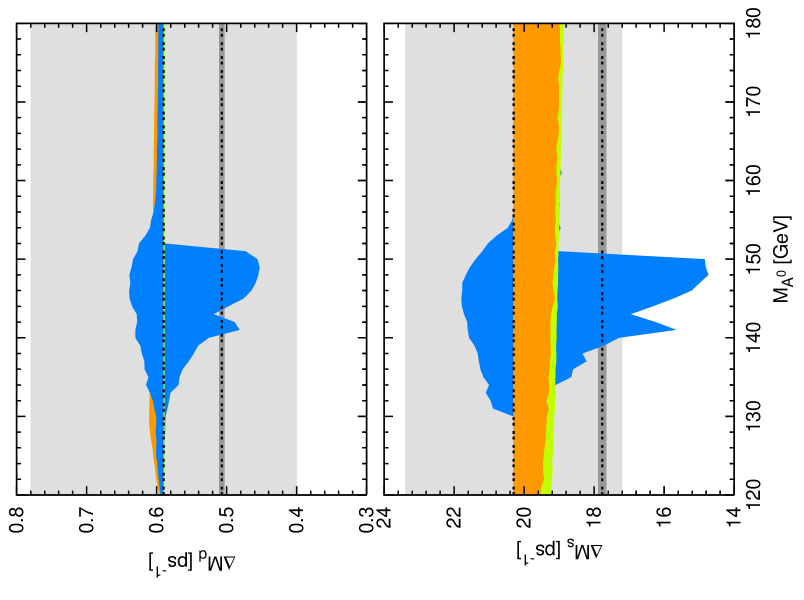
Figure 2: $\Delta M_{d}$ ($\Delta M_{s}$) as a function of $M_{A^{0}}$. The blue (dark gray) areas correspond to the improved predictions, while the orange (medium gray) and yellow-green (light gray) regions are obtained by neglecting sequentially the contributions due to $\epsilon_{\rm GP}$ and the one-loop corrections to $\alpha$, $M_{h^{0}}$, and $M_{H^{0}}$. The $1\hskip 1.13809pt\sigma$ ranges and central values of the experimental (SM) results are indicated by the dark (light) gray bands underlying the dotted lines. See text for details.

In our numerical analysis we focus on scenarios with heavy sparticles and the mass scale of the Higgs sector close to the electroweak scale. We allow the parameters to float freely in the following ranges: $10\leq\tan\beta\leq 60$, $100\hskip 1.42262pt{\rm GeV}\leq M_{A^{0}}\leq 500\hskip 1.42262pt{\rm GeV}$, $1\hskip 1.42262pt{\rm TeV}\leq\tilde{m}_{i}\leq 2\hskip 1.42262pt{\rm TeV}$ where $\tilde{m}_{i}=m_{\tilde{t}_{L}},m_{\tilde{t}_{R}},m_{\tilde{b}_{R}},m_{\tilde{\tau}_{L}},m_{\tilde{\tau}_{R}},M_{1},M_{2},M_{\tilde{g}}$, and $1\hskip 1.42262pt{\rm TeV}\leq|\tilde{M}_{i}|\leq 2\hskip 1.42262pt{\rm TeV}$ for $\tilde{M}_{i}=\mu,A_{t},A_{b},A_{\tau}$. The SM parameters are fixed to $\alpha_{s}=\alpha^{\overline{\rm MS}}_{s}(\overline{m}_{t})=0.109$, $\overline{m}_{t}=165\ {\rm GeV}$, $\overline{m}_{b}=3\ {\rm GeV}$, $\overline{m}_{s}=0.06\ {\rm GeV}$, $\overline{m}_{d}=0.003\ {\rm GeV}$, $\overline{m}_{\tau}=1.78\ {\rm GeV}$, $\alpha_{\rm em}=\alpha^{\overline{\rm MS}}_{\rm em}(M_{Z})=1/127.9$, and $s^{2}_{W}=\sin^{2}\hat{\theta}_{W}=0.231$ Yao:2006px . In order to find the boundaries of the allowed parameter space we perform an adaptive scan of the 14 SUSY variables employing the method advocated in adaptive . The correctness of the obtained results has been independently verified by a scanning procedure based on random walk techniques.

To simplify our numerical analysis we set all CKM factors and non-perturbative parameters to their central values and combine experimental and theoretical uncertainties into bounds corresponding to $95\%$ confidence levels (CLs) by adding theory errors linearly. Severe constraints on the SUSY parameter space follow from ${\cal B}(\bar{B}\to X_{s}\gamma)$, ${\cal B}(B_{s}\to\mu^{+}\mu^{-})$, ${\cal B}(B^{+}\to\tau^{+}\nu_{\tau})$, and $M_{h^{0}}$. In the case of $\bar{B}\to X_{s}\gamma$ the most recent SM calculations bsg are used and ${\cal B}(\bar{B}\to X_{s}\gamma)$ is required to lie in the interval $2.7\leq{\cal B}(\bar{B}\to X_{s}\gamma)\times 10^{4}\leq 4.4$. Since the SM prediction of ${\cal B}(\bar{B}\to X_{s}\gamma)$ is now lower than the experimental world average Barberio:2006bi by about $1.4\hskip 1.13809pt\sigma$, a cancellation between the constructive charged Higgs corrections and the chargino contribution is easier to achieve than in the past, where the theoretical result used to be above the experimental one. As far as $B_{s}\to\mu^{+}\mu^{-}$ is concerned all parameter points are required to satisfy ${\cal B}(B_{s}\to\mu^{+}\mu^{-})<1.0\times 10^{-7}$ Bernhard:2006fa , while, in view of the sizable experimental Btaunu and theoretical uncertainties, we use $0.2\leq{\cal B}(B^{+}\to\tau^{+}\nu_{\tau})\times 10^{4}\leq 2.5$ in the case of $B^{+}\to\tau^{+}\nu_{\tau}$. Because the interference between SM and charged Higgs corrections is necessarily destructive Hou:1992sy , $B^{+}\to\tau^{+}\nu_{\tau}$ may become the most stringent constraint in the near future, in particular if improved measurements of ${\cal B}(B^{+}\to\tau^{+}\nu_{\tau})$ will not differ much from the SM expectation. Finding ${\cal B}(B^{+}\to\tau^{+}\nu_{\tau})$ close to its SM prediction would also have a important effect on our numerical analysis since light values of $M_{A^{0}}$ would be disfavored in such a case. Concerning the lightest neutral Higgs boson we ensure $M_{h^{0}}>114.4\hskip 1.42262pt{\rm GeV}$ ewpm .

The constraints from $K$- and the remaining $B$-physics observables are much less restrictive. $\Delta M_{K}$ and $|\epsilon_{K}|$ are allowed to differ from their experimental values Yao:2006px by $\pm 50\%$ and $\pm 40\%$, while we reject parameter points that reverse the sign of the amplitude ${\cal A}(b\to s\gamma)$ with respect to the SM, as they correspond to ${\cal B}(\bar{B}\to X_{s}l^{+}l^{-})$ values higher than the measurements bxsll by around $3\hskip 1.13809pt\sigma$ Gambino:2004mv . In the case of $B_{d}\to\mu^{+}\mu^{-}$ we require ${\cal B}(B_{d}\to\mu^{+}\mu^{-})<3.0\times 10^{-8}$ Bernhard:2006fa . Notice that, we do not take into account the experimental constraint from $(g-2)_{\mu}$, because in our scenario the slepton sector parameters are uncorrelated with the ones of the squark sector, so that $(g-2)_{\mu}$ does not lead to any restriction.

The MFV MSSM prediction for the mass differences $\Delta M_{d,s}$ as a function of $M_{A^{0}}$ can be seen in Fig. 2. The blue (dark gray) areas correspond to the full results obtained from Eqs. (17) to (20), while the orange (medium gray) and yellow-green (light gray) regions are obtained after removing successively the contributions due to $\epsilon_{\rm GP}$ and the one-loop corrections to $\alpha$, $M_{h^{0}}$, and $M_{H^{0}}$. For comparison, the $68\%\ {\rm CLs}$ and central values of the measurements $\Delta M_{d}^{\rm exp}=0.507(4)\hskip 1.42262pt{\rm ps}^{-1}$ Barberio:2006bi and $\Delta M_{s}^{\rm exp}=17.77(12)\hskip 1.42262pt{\rm ps}^{-1}$ Abulencia:2006ze and the SM expectations $\Delta M_{d}^{\rm SM}=0.59(19)\hskip 1.42262pt{\rm ps}^{-1}$ and $\Delta M_{s}^{\rm SM}=20.3(3.1)\hskip 1.42262pt{\rm ps}^{-1}$ Dalgic:2006gp are indicated by the dark and light gray bands underlying the dotted lines. The prediction $\Delta M_{d}^{\rm SM}$ is obtained from the central value of $\Delta M_{s}^{\rm SM}$ using $\xi=f_{B_{s}}\hat{B}_{B_{s}}^{1/2}/(f_{B_{d}}\hat{B}_{B_{d}}^{1/2})=1.216(41)$ Okamoto:2005zg and the CKM factors and $B_{d,s}$-meson masses given earlier by adding all errors in quadrature. For a critical discussion of hadronic uncertainties in $\Delta M_{d,s}^{\rm SM}$ we refer to Ball:2006xx .

From Fig. 2 it is evident that, whereas one-loop corrections to $\alpha$, $M_{h^{0}}$, and $M_{H^{0}}$ have only a minor impact on $\Delta M_{s}$, which slowly loses importance with increasing $M_{A^{0}}$, they are essential to obtain a correct prediction in the case of $\Delta M_{d}$. While already this result is interesting by itself, truly spectacular effects arise after the inclusion of the new term $\epsilon_{\rm GP}$. Now large negative and positive corrections to $\Delta M_{d}$ ($\Delta M_{s}$) of up to $-0.14\hskip 1.42262pt{\rm ps}^{-1}$ and $0.05\hskip 1.42262pt{\rm ps}^{-1}$ ($-5.6\hskip 1.42262pt{\rm ps}^{-1}$ and $1.5\hskip 1.42262pt{\rm ps}^{-1}$) are possible in the mass window $130\hskip 1.42262pt{\rm GeV}\lesssim M_{A^{0}}\lesssim 160\hskip 1.42262pt{\rm GeV}$ without violating any existing constraint from flavor and collider physics. These large corrections typically arise for $15\lesssim\tan\beta\lesssim 30$ and $\mu,A_{t}\gtrsim 1.5\hskip 1.42262pt{\rm GeV}$. Their size is (slightly) less pronounced for larger (smaller) values of $m_{\tilde{t}_{L}}$ and $m_{\tilde{t}_{R}}$ ($M_{\tilde{g}}$), while they are highly uncorrelated with the remaining SUSY parameters. Therefore they do not correspond to exceptional points in the large $\tan\beta$ and small $M_{A^{0}}$ region of the MSSM parameter space.

As pointed out above, the small $M_{A^{0}}$ region may be severly constrained by a more precise determination of ${\cal B}(B^{+}\to\tau^{+}\nu_{\tau})$. The large effects shown in Fig. 2 occur only for ${\cal B}(B^{+}\to\tau^{+}\nu_{\tau})\lesssim 10^{-4}$. If future measurements should find a value in the ballpark of $1.5\times 10^{-}4$ with a small error of 30% or less, large corrections to $\Delta M_{d,s}$ would be excluded within the MSSM with MFV.

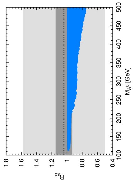
Figure 3: $R_{sd}^{\rm DP}$ as a function of $M_{A^{0}}$. The blue (dark gray) area corresponds to the improved MFV MSSM prediction. The $1\hskip 1.13809pt\sigma$ range and central value of the present (a possible future) tree-level prediction $R_{sd}^{\rm exp}$ corresponding to $\gamma=67(31)^{\circ}$ ($\gamma=67(5)^{\circ})$ is indicated by the light (dark) gray band and the dotted horizontal line. See text for details.

It is also compelling to analyze the impact of neutral Higgs DP contributions in the double ratio $R_{sd}^{\rm DP}=(\Delta M_{s}^{\rm DP}/\Delta M_{s}^{\rm SM})/(\Delta M_{d}^{\rm DP}/\Delta M_{d}^{\rm SM})$, which has smaller hadronic uncertainties than the ratios $\Delta M_{d,s}^{\rm DP}/\Delta M_{d,s}^{\rm SM}$ themselves. The size of the possible departures of $R_{sd}^{\rm DP}$ from the SM value $1$ should be compared to the total uncertainty of the double ratio

$$\begin{split}R_{sd}^{\rm exp}&=\lambda^{2}\left(1-2R_{b}\cos\gamma+R_{b}^{2}\right)\times\\ &\left(1+\left(1-2R_{b}\cos\gamma\right)\lambda^{2}\right)\frac{1}{\xi^{2}}\frac{M_{B_{d}}}{M_{B_{s}}}\frac{\Delta M_{s}^{\rm exp}}{\Delta M_{d}^{\rm exp}}\,,\hskip 14.22636pt\end{split}$$ (25)

that can be determined almost independently of new physics and $R_{b}=(1-\lambda^{2}/2)\hskip 1.42262pt1/\lambda\hskip 1.42262pt|V_{ub}^{\rm eff}/V_{cb}^{\rm eff}|$ Ball:2006xx from $\lambda=|V_{us}^{\rm eff}|$, $M_{B_{d,s}}$, $\Delta M_{d,s}^{\rm exp}$, $\xi$ and the reference unitarity triangle angle $\gamma$ measured in tree-level dominated $B$-decays like $B\to D^{(\ast)}K^{(\ast)}$.

The double ratio $R_{sd}^{\rm DP}$ as a function of $M_{A^{0}}$ is shown in Fig. 3, where the blue (dark gray) area represents the full result derived from Eqs. (17) to (20). The $68\%\ {\rm CL}$ and central value of the tree-level determination $R_{sd}^{\rm exp}=1.04(54)$ is indicated by the light gray band and the dotted line. The quoted range of $R_{sd}^{\rm exp}$ is obtained from Eq. (25) using $\lambda=0.2257(21)$, $R_{b}=0.42(4)$, $\gamma=67(31)^{\circ}$ Charles:2004jd and the remaining input specified above by adding all uncertainties in quadrature. Because of the poor knowledge of $\gamma$ from $B\to D^{(\ast)}K^{(\ast)}$ the double ratio $R_{sd}^{\rm exp}$ is only weakly constrained at the moment.

Two properties of $R_{sd}^{\rm DP}$ deserve a special mention. Our numerical analysis reveals that $i)$ effects due to $\epsilon_{\rm GP}$ and the one-loop corrections to $\alpha$, $M_{h^{0}}$, and $M_{H^{0}}$ cancel almost entirely in the double ratio $R_{sd}^{\rm DP}$ since their size is strongly correlated between $\Delta M_{d}^{\rm DP}$ and $\Delta M_{s}^{\rm DP}$ and $ii)$ the MFV MSSM with large $\tan\beta$ predicts $R_{sd}^{\rm DP}\leq 1$ as demonstrated in Fig. 3. The impact of a future precision measurement of $\gamma$ by the LHCb experiment LHCb is also illustrated in this figure. Assuming $\gamma=67(5)^{\circ}$ but $\xi$ unaltered leads to $R_{sd}^{\rm exp}=1.04(11)$. The corresponding $68\%\ {\rm CL}$ and central value is indicated by the dark gray band and the dotted line in Fig. 3. It can be seen that even with this improvement in precision, $R_{sd}^{\rm exp}$ offers only limited potential for exclusion of new physics through a deviation from its SM value. A similar conclusion has been drawn in Ball:2006xx .

V Conclusions

To conclude, we have pointed out that in the MSSM terms from the mixing between eigenstates of the two Higgs doublets give rise to $\tan\beta$ enhanced corrections that do not vanish in the limit where the SUSY particles are much heavier than the Higgs bosons. We have calculate all one-loop corrections of this type by matching the full MSSM on to an effective two-Higgs-doublet model of type II. After combining the missing effective couplings with all known non-holomorphic terms we obtain improved predictions for the $B_{d,s}\text{--}\bar{B}_{d,s}$ mass differences $\Delta M_{d,s}$ and the branching ratios of $B_{d,s}\to\mu^{+}\mu^{-}$ in the large $\tan\beta$ regime of the MSSM with minimal-flavor-violation. Our numerical analysis shows that these universal contributions have striking phenomenological implications as they can lead to large SUSY effects in $\Delta M_{d}$ and to a significant enhancement of $\Delta M_{s}$ relative to the SM prediction for a light pseudoscalar Higgs boson $A^{0}$ with mass in the range between $130\hskip 1.42262pt{\rm GeV}$ and $160\hskip 1.42262pt{\rm GeV}$.

References

(1)
L. J. Hall, R. Rattazzi and U. Sarid,
Phys. Rev. D 50, 7048 (1994).
(2)
M. Carena et al.,
Nucl. Phys. B 577, 88 (2000).
(3)
G. Degrassi, P. Gambino and G. F. Giudice,
JHEP 0012, 009 (2000);
M. Carena et al.,
Phys. Lett. B 499, 141 (2001).
(4)
T. Blazek, S. Raby and S. Pokorski,
Phys. Rev. D 52, 4151 (1995).
(5)
K. S. Babu and C. F. Kolda,
Phys. Rev. Lett. 84, 228 (2000).
(6)
U. Nierste, private communication (2003).
(7)
A. J. Buras et al.,
Nucl. Phys. B 619, 434 (2001);
Phys. Lett. B 546, 96 (2002);
Nucl. Phys. B 659, 3 (2003).
(8)
G. Isidori and A. Retico,
JHEP 0111, 001 (2001).
(9)
G. D’Ambrosio et al.,
Nucl. Phys. B 645, 155 (2002).
(10)
M. Carena et al.,
Phys. Rev. D 74, 015009 (2006).
(11)
M. Blanke et al.,
JHEP 0610, 003 (2006).
(12)
G. Isidori and P. Paradisi,
Phys. Lett. B 639, 499 (2006);
E. Lunghi, W. Porod and O. Vives,
Phys. Rev. D 74, 075003 (2006).
(13)
A. Freitas and D. Stöckinger,
Phys. Rev. D 66, 095014 (2002).
(14)
C. Hamzaoui, M. Pospelov and M. Toharia,
Phys. Rev. D 59, 095005 (1999);
C. S. Huang et al.,
Phys. Rev. D 63, 114021 (2001)
[Erratum-ibid. D 64, 059902 (2001)];
P. H. Chankowski and L. Slawianowska,
Phys. Rev. D 63, 054012 (2001);
C. Bobeth et al.,
Phys. Rev. D 64, 074014 (2001);
A. Dedes, H. K. Dreiner and U. Nierste,
Phys. Rev. Lett. 87, 251804 (2001);
A. Dedes and A. Pilaftsis,
Phys. Rev. D 67, 015012 (2003);
J. Foster, K. i. Okumura and L. Roszkowski,
Phys. Lett. B 609, 102 (2005);
JHEP 0508, 094 (2005);
Phys. Lett. B 641, 452 (2006).
(15)
R. Barbieri and M. Frigeni,
Phys. Lett. B 258, 395 (1991);
J. R. Ellis, G. Ridolfi and F. Zwirner,
Phys. Lett. B 262, 477 (1991);
A. Brignole et al.,
Phys. Lett. B 271, 123 (1991).
(16)
A. J. Buras, M. Misiak and J. Urban,
Nucl. Phys. B 586, 397 (2000).
(17)
D. Becirevic et al.,
JHEP 0204, 025 (2002).
(18)
A. Gray et al. [HPQCD Collaboration],
Phys. Rev. Lett. 95, 212001 (2005)
(19)
M. Wingate et al.,
Phys. Rev. Lett. 92, 162001 (2004).
(20)
P. Ball and R. Fleischer,
Eur. Phys. J. C 48, 413 (2006).
(21)
W. M. Yao et al. [Particle Data Group],
J. Phys. G 33 (2006) 1.
(22)
C. Bobeth et al.,
JHEP 0404, 071 (2004).
(23)
E. Barberio et al. [Heavy Flavor Averaging Group (HFAG)],
hep-ex/0603003, and online update available at
http://www.slac.stanford.edu/xorg/hfag.
(24)
A. G. Akeroyd and S. Recksiegel,
J. Phys. G 29, 2311 (2003).
(25)
J. K. Parry,
Mod. Phys. Lett. A 21, 2853 (2006).
(26)
O. Brein,
Comput. Phys. Commun. 170, 42 (2005);
A. J. Buras et al.,
Nucl. Phys. B 714, 103 (2005).
(27)
M. Misiak et al.,
Phys. Rev. Lett. 98, 022002 (2007);
M. Misiak and M. Steinhauser,
Nucl. Phys. B 764, 62 (2007);
T. Becher and M. Neubert,
Phys. Rev. Lett. 98, 022003 (2007).
(28)
R. P. Bernhard,
hep-ex/0605065.
(29)
K. Ikado et al.,
Phys. Rev. Lett. 97, 251802 (2006);
B. Aubert [BABAR Collaboration],
hep-ex/0608019.
(30)
W. S. Hou,
Phys. Rev. D 48, 2342 (1993).
(31)
S. Schael et al.,
Phys. Rept. 427, 257 (2006).
(32)
B. Aubert et al. [BaBar Collaboration],
Phys. Rev. Lett. 93, 081802 (2004);
K. Abe et al. [Belle Collaboration],
hep-ex/0408119.
(33)
P. Gambino, U. Haisch and M. Misiak,
Phys. Rev. Lett. 94, 061803 (2005).
(34)
A. Abulencia et al. [CDF Collaboration],
Phys. Rev. Lett. 97, 242003 (2006).
(35)
E. Dalgic et al.,
hep-lat/0610104.
(36)
M. Okamoto,
PoS LAT2005, 013 (2006).
(37)
J. Charles et al. [CKMfitter Group],
Eur. Phys. J. C 41, 1 (2005),
and online update available at http://ckmfitter.in2p3.fr/.
(38)
O. Schneider, talk at the “Flavour in the era of the LHC” workshop,
CERN, November 2005, http://cern.ch/flavlhc.