Abstract

Massive on–shell operator matrix elements and self-energy diagrams with outer gluon lines are calculated analytically at $O(\alpha_{s}^{2})$, using Mellin–Barnes integrals and representations through generalized hypergeometric functions. This method allows for a direct evaluation without decomposing the integrals using the integration-by-parts method.

1 Introduction

In the asymptotic region $Q^{2}\gg m^{2}$, the heavy flavor contributions to the deeply inelastic structure functions can be obtained from the corresponding massive operator matrix elements and the light flavor Wilson coefficients [1]. The massless Wilson coefficients for deeply inelastic scattering are known up to 3–loop order [2, 3]. The heavy flavor contributions were calculated to next-to-leading order in [4] semi-analytically. A fast numerical implementation was given in [5]. Complete analytic results were derived only for the limit $Q^{2}\gg m^{2}$ for the structure function $F_{2}^{Q\overline{Q}}(x,Q^{2})$ to $O(\alpha_{s}^{2})$ [1] and $F_{L}^{Q\overline{Q}}(x,Q^{2})$ to $O(\alpha_{s}^{3})$ [6]. In both cases, the $O(\alpha_{s}^{2})$ massive operator matrix elements are required. The asymptotic contributions cover all logarithmic and the constant terms, while contributions of $O((m^{2}/Q^{2})^{k}),~{}k\geq 1$ are not contained. In the case of the structure function $F_{2}(x,Q^{2})$, these terms yield a very good description already in the region $Q^{2}\raisebox{-1.9919pt}{$\,\stackrel{{\scriptstyle>}}{{{\scriptstyle\sim}}}\,$}20\,\mbox{GeV}^{2}$, while for $F_{L}(x,Q^{2})$ this approximation only holds at large scales $Q^{2}\raisebox{-1.9919pt}{$\,\stackrel{{\scriptstyle>}}{{{\scriptstyle\sim}}}\,$}1000\,\mbox{GeV}^{2}$. Since the heavy flavor contributions to the structure functions amount to 20–40 % in the small $x$ region, cf. [7], and the scaling violations of these terms differ from that of the light parton contributions, their knowledge is essential for precision measurements of the QCD scale $\Lambda_{\rm QCD}$ in singlet analyses.

In this letter we address a new compact calculation of the genuine 2–loop scalar integrals contributing to the massive operator matrix elements with outer gluon lines, based on the Mellin-Barnes technique [8, 9, 10] and using representations through generalized hypergeometric functions [11]. This approach allows to thoroughly avoid the use of the integration-by-parts method [12], which keeps the contributing number of terms low and yields very compact results. Moreover, we work in Mellin space to use the appropriate symmetry of the problem leading to further compactification. The complete calculation of the asymptotic heavy flavor Wilson coefficients will be presented elsewhere [13]. In the following, we will outline the principal method and present then the results for the seven contributing two–loop integrals in terms of nested harmonic sums [14, 15]. Some of the special sums needed are listed in the appendix.

2 The Method

The massive 2–loop diagrams considered are shown in Figure 1.

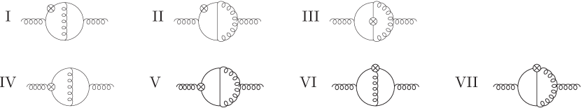
Figure 1: Genuine 2-loop diagrams contributing to the massive operator matrix elements.

The diagrams contain either three or four massive lines. The $\otimes$–symbol in Figure 1 denotes the operator insertion of the corresponding local quark-gluon operators, see Figure 2.

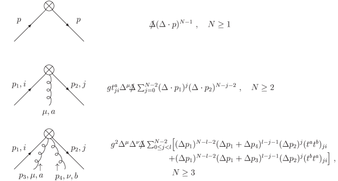
Figure 2: QCD Feynman rules for the composite local operator insertions.

The diagrams can be decomposed into a *–product as described in Figure 3. We follow the calculation of Ref. [10], now generalized from massless self–energy diagrams to massive operator matrix elements.

0.6 1                                                               0.6 1          

0.55 1.5

=

0.55 1.5

$\ast$ 0.55 1.5

Figure 3: The massive two–loop two–point diagrams with three and four fermion masses. The graphs are generated by inserting the three–point function, written as a double Mellin–Barnes integral, into the massive two–point function, i.e. performing the $\ast$-operation defined in the context of the Lie–algebra of Feynman diagrams [16]. The effect of this insertion is only given by a modification of the exponents of the two–point function, cf. [10].

Also in this case the above decomposition of diagrams can be achieved by applying the Mellin–Barnes representation 

$$\frac{1}{(A_{1}+A_{2})^{\nu}} = \frac{1}{2\pi i}\int_{\gamma-i\infty}^{\gamma+i\infty}d\sigma\>A_{1}^{\sigma}A_{2}^{-\nu-\sigma}\frac{\Gamma(-\sigma)\Gamma(\nu+\sigma)}{\Gamma(\nu)}~{}.$$ (1)

Let us consider Diagram I as an example. The corresponding gluing-product is depicted in Figure 4. Applying the Feynman-parameterization to the 2-point function yields

$${I}^{(1,2)} = \frac{\Gamma(\nu_{14})}{\Gamma(\nu_{1})\Gamma(\nu_{4})}~{}{(m^{2})^{\nu_{14}-D/2}}{(4\pi)^{2}}\int_{0}^{1}dx_{1}dx_{2}x_{1}^{\nu_{1}-1}x_{2}^{\nu_{4}-1}\delta(x_{1}+x_{2}-1)$$

$$\times\int\frac{d^{D}k_{1}}{(2\pi)^{D}}\frac{(\Delta.k_{1})^{N-1}}{(x_{1}k_{1}^{2}+x_{1}m^{2}+x_{2}(k_{1}-p)^{2}+x_{2}m^{2})^{\nu_{14}}}~{}.$$ (2)

Here, $\Delta$ denotes a light-like vector with $\Delta^{2}=0$, and $D=4-2\varepsilon$. $\nu_{i}$ is the integer power of the respective propagator and $\nu_{ij\ldots}=\nu_{i}+\nu_{j}+\ldots$ . The calculation is performed in the $\overline{\rm MS}$ scheme and we factor out $S_{\varepsilon}=\exp[\varepsilon(\ln(4\pi)-\gamma_{E})]$ for each loop.  One shifts $k_{1}\rightarrow k_{1}+x_{2}p$ and the numerator term is decomposed as

$$(\Delta.k_{1}+x_{2}\Delta.p)^{N}=\sum_{l=0}^{N}\binom{N}{l}(\Delta.k_{1})^{l}(x_{2}\Delta.p)^{N-l}~{}.$$ (3)

All integrals over $k_{1}$ with $(\Delta.k_{1})^{l},~{}l\geq 1$ vanish.

Figure 4: Diagram insertion for graph I.

One obtains

$${I}^{(1,2)} = (\Delta.p)^{N-1}(4\pi)^{\varepsilon}\frac{\Gamma(\nu_{14}-D/2)\Gamma(\nu_{4}+N-1)}{\Gamma(\nu_{4})\Gamma(\nu_{14}+N-1)}~{}.$$ (4)

In the next step, the three-point function is inserted in a similar way as in [10], since a part of the propagators are massive but no operator insertion occurs. The result for diagram I for $\nu_{i}=1,\forall i$, can be expressed by a double Mellin–Barnes integral as

$${I}_{1} = \frac{(4\pi)^{2\varepsilon}}{(2\pi)^{2}}\frac{(\Delta.p)^{N-1}}{\Gamma(1-2\varepsilon)}$$ (5)

$$\times\int_{\gamma_{1}-i\infty}^{\gamma_{1}+i\infty}d\sigma\int_{\gamma_{2}-i\infty}^{\gamma_{2}+i\infty}d\tau\>\frac{\Gamma(-\sigma)\Gamma(\sigma+1)\Gamma(-\sigma+N)}{\Gamma(-\sigma+1)}\Gamma(-\tau)\Gamma(\tau+1)$$

$$\times\frac{\Gamma(\sigma+\tau+1)\Gamma(\sigma+\tau+1+\varepsilon)\Gamma(-\sigma-\tau-2\varepsilon)\Gamma(-\sigma-\tau+\varepsilon)}{\Gamma(\sigma+\tau+2)\Gamma(-\sigma-\tau+1+N)}~{}.$$

The other six 2-loop integrals obey a similar representation. For fixed values of $N$, one may calculate the Mellin–Barnes integrals using the mathematica–package MB by M. Czakon [20], which yields numerical values. They were given in Ref. [21], Table 1. 

For the solution of one of the Mellin-Barnes integrals, relations like

$$\frac{1}{2\pi i}\int_{\gamma-i\infty}^{\gamma+i\infty}ds\frac{\Gamma(a+s)\Gamma(b+s)\Gamma(d-a-b-s)\Gamma(e-c+s)\Gamma(-s)}{\Gamma(e+s)}$$ (6)

$$\hskip 113.81102pt=\frac{\Gamma(e-c)\Gamma(a)\Gamma(b)\Gamma(d-a)\Gamma(d-b)}{\Gamma(e)\Gamma(d)}~{}_{3}F_{2}[a,b,c;d,e;1]~{},$$

cf. [11], are used. The second integral is performed by applying the residue theorem. One obtains

$${I}_{1} = (\Delta\cdot p)^{N-1}\>(4\pi)^{2\varepsilon}\frac{\Gamma(N+1)}{\Gamma(1-2\varepsilon)}\>\sum_{k=0}^{\infty}\sum_{j=0}^{\infty}\frac{\Gamma(k+1)}{\Gamma(k+2+N)}$$ (7)

$$\times\Biggl{[}\Gamma(\varepsilon)\Gamma(1-\varepsilon)\frac{\Gamma(j+1-2\varepsilon)\Gamma(j+1+\varepsilon)}{\Gamma(j+1-\varepsilon)\Gamma(j+2+N)}\frac{\Gamma(k+j+1+N)}{\Gamma(k+j+2)}$$

$$+\Gamma(-\varepsilon)\Gamma(1+\varepsilon)\frac{\Gamma(j+1+2\varepsilon)\Gamma(j+1-\varepsilon)}{\Gamma(j+1)\Gamma(j+2+\varepsilon+N)}\frac{\Gamma(k+j+1+\varepsilon+N)}{\Gamma(k+j+2+\varepsilon)}\Biggr{]}~{}.$$

One first performs the $\varepsilon$–expansion to the desired order. The infinite sums in (7) can be expressed through Mellin-type integral representations, partly using differential operators in the remaining summation and outer parameters. In some cases the starting values $\{k,j\}=0$ need a separate treatment. The corresponding Mellin-integrals finally result into weighted harmonic sums. The calculations were coded in MAPLE. For fixed values of $N$, simpler procedures are obtained which lead to analytic expressions for the expansion coefficients in $\varepsilon$, cf. Table 2, Ref. [21].

Except for diagrams VI, VII one may calculate the integrals in the above way for general values of $N$.

Explicit representations for all diagrams could be derived using generalized hypergeometric functions for all diagrams. As an example, let us consider diagram VI,

$$I_{6} = \int\!\!\frac{dk_{1}}{(2\pi)^{D}}\int\!\!\frac{dk_{2}}{(2\pi)^{D}}\frac{(\Delta k_{1})^{N-1}\!-\!(\Delta k_{2})^{N-1}}{(\Delta k_{1}\!-\!\Delta k_{2})}$$

$$\times(4\pi)^{4}~{}\frac{(m^{2})^{1+2\varepsilon}}{(k_{1}^{2}\!-\!m^{2})((k_{1}\!-\!p)^{2}\!-\!m^{2})(k_{2}^{2}\!-\!m^{2})((k_{2}\!-\!p)^{2}\!-\!m^{2})^{2}(k_{2}\!-\!k_{1})^{2}}$$

$$= (\Delta p)^{N-2}\Gamma(1+2\varepsilon)(4\pi)^{2\varepsilon}\frac{2\pi}{N\sin(-\pi\varepsilon)}\sum_{j=1}^{N}\Biggl{\{}\binom{N}{j}(-1)^{j}+\delta_{j,N}\Biggr{\}}$$

$$\times\Biggl{\{}\frac{\Gamma(j)\Gamma(j+1+\varepsilon)}{\Gamma(j+2+2\varepsilon)\Gamma(j+1-\varepsilon)}-\frac{B(1+\varepsilon,1+j)}{j}~{}_{3}F_{2}\left[1+2\varepsilon,-\varepsilon,j+1;1,j+2+\varepsilon;1\right]\Biggr{\}}~{}.$$

After performing the expansion in $\varepsilon$, the remaining sums can be carried out by suitable integral representations. Some of the sums required are listed in the appendix.

3 Results

All diagrams obey representations in terms of weighted harmonic sums in the present case. It even turns out that only single harmonic sums contribute. Not all the diagrams I–VII are independent. Due to the massless outer lines of the diagrams, graphs IV and V can be expressed in terms of diagrams ${\rm I}_{a}$ and II. Here ${\rm I}_{a}$ corresponds to the case where all scalar propagators have power one, i.e.

$${\rm IV} = \left[1+(-1)^{N}\right]\frac{1}{\Delta.p}\times{\rm I}_{a}$$ (9)

$${\rm V} = \left[1+(-1)^{N}\right]\frac{1}{\Delta.p}\times{\rm II}$$ (10)

For diagram III, even a closed expression for general values of $\varepsilon$ can be derived,

$$I_{3} = \int\!\!\!\frac{dk_{1}}{(2\pi)^{D}}\int\!\!\!\frac{dk_{2}}{(2\pi)^{D}}\frac{(4\pi)^{4}(\Delta k_{1}\!-\!\Delta k_{2})^{N-1}\quad(m^{2})^{1+2\varepsilon}}{(k_{1}^{2}\!-\!m^{2})((k_{1}\!-\!p)^{2}\!-\!m^{2})((k_{1}\!-\!k_{2})^{2}\!-\!m^{2})k_{2}^{2}(k_{2}\!-\!p)^{2}}$$

$$= (\Delta p)^{N-1}\Gamma(1+2\varepsilon)(4\pi)^{2\varepsilon}\frac{\pi}{\sin(-\pi\varepsilon)}\frac{1-(-1)^{N}}{N(N+1)}\frac{\Gamma(N+1+\varepsilon)\Gamma(N+1)}{\Gamma(N+2+2\varepsilon)\Gamma(N+1-\varepsilon)}$$

$$= (\Delta p)^{N-1}\Gamma(1+2\varepsilon)(4\pi)^{2\varepsilon}\frac{1-(-1)^{N}}{N(N+1)^{2}}\Biggl{[}-\frac{1}{\varepsilon}+\frac{2}{N+1}\Biggr{]}+O(\varepsilon).$$

We summarize the results for the independent diagrams I-III,VI,VII in Table 1, expanding to $O(\varepsilon^{0})$ in the $\overline{\rm MS}$–scheme. The expressions in terms of harmonic sums were derived exploiting their algebraic relations [23].

Table 1: The analytic results for graphs I to VII for general values of N, with all $\nu_{i}=1$, Ib: $\nu_{1}=2$.

$\rm{Ia}$	$\displaystyle\frac{{S}_{1}^{2}({N})+3{S}_{2}({N})}{2{N}({N}+1)}$
$\rm{Ib}$	$\displaystyle\frac{{S}_{1}({N})-3S_{2}(N)/2-S_{1}^{2}(N)/2}{{N}({N}+1)(N+2)}-\frac{1}{(N+1)^{2}(N+2)}$
$\rm{II}$	$\displaystyle\frac{{S}_{1}({N})}{{N}({N}+1)}\left(-\frac{1}{\varepsilon}\right)+2\frac{{S}_{1}({N})}{{N}({N}+1)^{2}}+\frac{{S}_{1}^{2}({N})-{S}_{2}({N})}{2{N}({N}+1)}$
$\rm{III}$	$\displaystyle\frac{[1-(-1)^{{N}}]}{{N}({N}+1)^{2}}\left(-\frac{1}{\varepsilon}+\frac{2}{({N}+1)}\right)$
$\rm{VI}$	$\displaystyle\frac{4}{N}\left[S_{2}(N)-\frac{S_{1}(N)}{N}\right]$
$\rm{VII}$	$\displaystyle\left[\frac{(-1)^{N}-1}{N^{2}(N+1)}+\frac{2S_{1}(N)}{N(N+1)}\right]\left(-\frac{1}{\varepsilon}\right)$
	$\displaystyle+\left[2\frac{(-1)^{N}-1}{N^{2}(N+1)^{2}}+\frac{S_{1}^{2}(N)-S_{2}(N)+2S_{-2}(N)}{N(N+1)}+\frac{2(3N+1)S_{1}(N)}{N^{2}(N+1)^{2}}\right]$

In terms of (single) harmonic sums

$$S_{a}(N)=\sum_{k=1}^{N}\frac{({\rm sign}(a))^{k}}{k^{|a|}}~{},$$ (12)

the final expressions for the genuine 2–loop diagrams turn out to be extraordinarily simple. Due to the fact that we were not applying the integration-by-parts method, also the intermediary results remained rather compact. The results may be translated into $x$-space by inverse Mellin transformation using the Tables in [14]. On the other hand, one may work within the Mellin space representation continuing the expressions to complex values of $N$ as described in [24] and construct the respective observables in analytic form. The inverse Mellin transformation is then performed by a single numeric integral.

The diagrams are applied to express the unpolarized massive 2–loop operator matrix elements [1, 13]. As shown in [6, 13], nested harmonic sums will contribute in the physical result but they are either due to one-loop insertions into one-loop diagrams or the four-propagator contributions to some of the topologies discussed here, which are obtained due to cancellation of numerator and denominator terms.

4 Appendix

We list some special sums which are typical for classes of sums to be derived for the present calculation.

$$\sum_{k=1}^{\infty}\sum_{i=1}^{\infty}\frac{S_{1}(k+i+N)}{(k+i)(N+k)k} = \frac{1}{2}\sigma_{1}^{2}\frac{S_{1}(N)}{N}+2\frac{S_{1,1}(N)}{N^{2}}-\frac{\zeta_{2}}{2}\frac{S_{1}(N)}{N}-\frac{2\zeta_{3}}{N}$$ (13)

$$\sum_{i=1}^{\infty}\frac{B(N,i)}{i} = \zeta_{2}-S_{2}(N-1)$$ (14)

$$\sum_{i=1}^{\infty}\frac{B(N+1,i)}{(N+i)} = (-1)^{N}\left[2S_{-2}(N)+\zeta_{2}\right]$$ (15)

$$\sum_{i=1}^{\infty}\frac{B(N,i)}{(N+i+1)^{2}} = \frac{(-1)^{N}}{N(N+1)}\left[2S_{-2}(N)+\zeta_{2}\right]+\frac{N-1}{N(N+1)^{3}}$$ (16)

$$\sum_{i=1}^{\infty}\frac{B(N+1,i)S_{1}(i)}{(N+i)} = \frac{\zeta_{2}-S_{2}(N)}{N}+(-1)^{N}\Biggl{[}\zeta_{3}+S_{-3}(N)-2\frac{S_{-2}(N)}{N}$$ (17)

$$+2S_{1,-2}(N)-\frac{\zeta_{2}}{N}+\zeta_{2}S_{1}(N)\Biggr{]}$$

$$\sum_{k=0}^{N-1}\binom{N-1}{k}(-1)^{k}\frac{S_{1}^{2}(k+2)}{k+2} = -\frac{2N+1}{N^{2}(N+1)^{2}}S_{1}(N)+\frac{N^{3}+6N^{2}+6N+2}{N^{3}(N+1)^{3}}$$ (18)

$$\sum_{k=0}^{L}\binom{L+1}{k}\frac{(-1)^{k}}{(N-L+k)^{2}} = B(N-L,L+2)\left[S_{1}(N+L)-S_{1}(N-L-1)\right]~{}.$$ (19)

Here the symbol $\sigma_{1}$ and Euler’s Beta-function $B(a,b)$ are defined by

$$\sigma_{1} = \lim_{N\rightarrow\infty}S_{1}(N)$$ (20)

$$B(a,b) = \frac{\Gamma(a)\Gamma(b)}{\Gamma(a+b)}~{}.$$ (21)

References

- [1] M. Buza, Y. Matiounine, J. Smith, R. Migneron and W. L. van Neerven, Nucl. Phys. B 472 (1996) 611 [arXiv:hep-ph/9601302].
-
[2]
D. W. Duke, J. D. Kimel and G. A. Sowell,
Phys. Rev. D 25 (1982) 71;
A. Devoto, D. W. Duke, J. D. Kimel and G. A. Sowell, Phys. Rev. D 30 (1984) 541;
D. I. Kazakov and A. V. Kotikov, Nucl. Phys. B 307 (1988) 721 [Erratum-ibid. B 345 (1990) 299]; Phys. Lett. B 291 (1992) 171;
D. I. Kazakov, A. V. Kotikov, G. Parente, O. A. Sampayo and J. Sanchez Guillen, Phys. Rev. Lett. 65 (1990) 1535;
J. Sanchez Guillen, J. Miramontes, M. Miramontes, G. Parente and O. A. Sampayo, Nucl. Phys. B 353 (1991) 337;
S. A. Larin and J. A. M. Vermaseren, Z. Phys. C 57 (1993) 93;
W. L. van Neerven and E. B. Zijlstra, Phys. Lett. B 272 (1991) 127;
E. B. Zijlstra and W. L. van Neerven, Phys. Lett. B 273 (1991) 476; Nucl. Phys. B 383 (1992) 525;
S. Moch and J. A. M. Vermaseren, Nucl. Phys. B 573 (2000) 853 [arXiv:hep-ph/9912355]. -
[3]
S. A. Larin, T. van Ritbergen and J. A. M. Vermaseren,
Nucl. Phys. B 427 (1994) 41;
S. A. Larin, P. Nogueira, T. van Ritbergen and J. A. M. Vermaseren, Nucl. Phys. B 492 (1997) 338 [arXiv:hep-ph/9605317];
A. Retey and J. A. M. Vermaseren, Nucl. Phys. B 604 (2001) 281 [arXiv:hep-ph/0007294]l;
J. Blümlein and J. A. M. Vermaseren, Phys. Lett. B 606 (2005) 130 [arXiv:hep-ph/0411111];
S. Moch, J. A. M. Vermaseren and A. Vogt, Phys. Lett. B 606 (2005) 123 [arXiv:hep-ph/0411112];
J. A. M. Vermaseren, A. Vogt and S. Moch, Nucl. Phys. B 724 (2005) 3 [arXiv:hep-ph/0504242]. 5 -
[4]
E. Laenen, S. Riemersma, J. Smith and W. L. van Neerven,
Nucl. Phys. B 392 (1993) 162;
229;
S. Riemersma, J. Smith and W. L. van Neerven, Phys. Lett. B 347 (1995) 143 [arXiv:hep-ph/9411431]. - [5] S. I. Alekhin and J. Blümlein, Phys. Lett. B 594 (2004) 299 [arXiv:hep-ph/0404034].
- [6] J. Blümlein, A. De Freitas, W. L. van Neerven and S. Klein, Nucl. Phys. B 755 (2006) 272 [arXiv:hep-ph/0608024].
-
[7]
M. Glück, E. Reya and M. Stratmann,
Nucl. Phys. B 422 (1994) 37;
J. Blümlein and S. Riemersma, arXiv:hep-ph/9609394. - [8] E.W. Barnes, Proc. Lond. Math. Soc. (2) 6 (1908) 141; E.W. Barnes, Quart. J. Math. 41 (1910) 136.
-
[9]
H. Mellin, Math. Ann. 68 (1910) 305;
E.T. Whittaker and G.N. Watson, A Course of Modern Analysis, (Cambridge University Press, Cambridge, 1927; reprinted 1996);
E.C. Titchmarsh, Introduction to the Theory of Fourier Integrals, (Oxford, Calendron Press, 1937; 2nd Edition 1948). - [10] I. Bierenbaum and S. Weinzierl, Eur. Phys. J. C 32 (2003) 67 [arXiv:hep-ph/0308311].
-
[11]
W.N. Bailey, Generalized Hypergeometric Series,
(Cambridge University Press, Cambridge, 1935);
L.J. Slater, Generalized Hypergeometric Functions, (Cambridge University Press, Cambridge, 1966). - [12] K. G. Chetyrkin, A. L. Kataev and F. V. Tkachov, Nucl. Phys. B 174 (1980) 345.
- [13] I. Bierenbaum, J. Blümlein, and S. Klein, in preparation.
- [14] J. Blümlein and S. Kurth, Phys. Rev. D 60 (1999) 014018 [arXiv:hep-ph/9810241].
- [15] J. A. M. Vermaseren, Int. J. Mod. Phys. A 14 (1999) 2037 [arXiv:hep-ph/9806280].
- [16] A. Connes and D. Kreimer, Annales Henri Poincare 3 (2002) 411 [arXiv:hep-th/0201157].
- [17] S. Pincherle, Atti d. R. Accademia dei Lincei, Series IV., Rendiconti, Vol. IV., pp. 694-700; 792–799.
- [18] B. Riemann, Mathematische Werke, 1892, pp. 145–147.
- [19] A. Kratzer and W. Franz, Transzendente Funktionen, (Akad. Verlagsgesellschaft Geest & Portig K.-G., Leipzig, 1963).
- [20] M. Czakon, Comput. Phys. Commun. 175 (2006) 559 [arXiv:hep-ph/0511200].
- [21] I. Bierenbaum, J. Blümlein and S. Klein, Nucl. Phys. Proc. Suppl. 160 (2006) 85 [arXiv:hep-ph/0607300].
- [22] S. Weinzierl, Comput. Phys. Commun. 145 (2002) 357 [arXiv:math-ph/0201011].
- [23] J. Blümlein, Comput. Phys. Commun. 159 (2004) 19 [arXiv:hep-ph/0311046].
-
[24]
J. Blümlein,
Comput. Phys. Commun. 133 (2000) 76
[arXiv:hep-ph/0003100];
J. Blümlein and S. O. Moch, Phys. Lett. B 614 (2005) 53 [arXiv:hep-ph/0503188].