SUSY-induced FCNC top-quark processes at the Large Hadron Collider

Abstract

We systematically calculate various flavor-changing neutral-current top-quark processes induced by supersymmetry at the Large Hadron Collider, which include five decay modes and six production channels. To reveal the characteristics of these processes, we first compare the dependence of the rates for these channels on the relevant supersymmetric parameters, then we scan the whole parameter space to find their maximal rates, including all the direct and indirect current experimental constraints on the scharm-stop flavor mixings. We find that, under all these constraints, only a few channels, through $cg\to t$ at parton-level and $t\to ch$, may be observable at the Large Hadron Collider.

I Introduction

The study of various flavor-changing neutral-current (FCNC) processes has been shown to be very useful. In particular, as the heaviest fermion in the standard model (SM), the top quark may play a special role in FCNC phenomenology. In the SM the FCNC interactions of the top quark are extremely suppressed by the GIM mechanism, so that no FCNC top quark rates can reach an observable level at current or future colliders tcvh-sm ; tcgg-sm ; eetc-sm . Thus, the observation of any FCNC top quark process would be a robust evidence for new physics beyond the SM. Due to its heaviness, the top quark is very sensitive to new physics. Indeed, several models beyond the SM often predict much larger FCNC top quark interactions Larios:2006pb . Such FCNC interactions can induce various top quark production and decay channels, which can be explored in future collider experiments Aguilar-Saavedra:2004wm ; Aguilar-saavedra:linear and serve as a good probe for new physics.

So far, much effort has been spent on the exploration of the FCNC top quark interactions. On the experimental side, the Tevatron CDF and D0 collaborations have reported interesting bounds on the FCNC top quark decays from Run 1 experiment and will tighten the bounds from the ongoing Run 2 experiments cdfd0 . On the theoretical side, various FCNC top quark decays and top-charm associated productions at high energy colliders were extensively studied in the SM tcvh-sm ; tcgg-sm ; eetc-sm , the Minimal Supersymmetric Standard Model (MSSM) tcv-mssm ; tch-mssm ; eetc-mssm ; pptc-mssm ; Gad-pptc-mssm and other new physics models tc-TC2 ; tcv-TC2 ; other . These studies showed that the SM predictions for such processes are far below the detectable level. However, some new physics can enhance them by several orders of magnitude, which makes them potentially accessible at future colliders.

The Large Hadron Collider (LHC) at CERN will be a powerful machine for studying the top quark properties such as its FCNC interactions since it will produce top quarks copiously. Analysis Aguilar-Saavedra:2004wm showed that some FCNC top quark rare decays with branching ratios as low as ${\cal O}(10^{-5})$ could be accessible at the LHC. Due to its high energy and high luminosity, the LHC will be the main utility for exploring FCNC top quark production channels Aguilar-Saavedra:2004wm .

The minimal supersymmetric standard model (MSSM) is a leading candidate for new physics beyond the SM and its consequences will be extensively explored at the LHC. In this paper, we throughly investigate various top quark FCNC processes in the framework of the MSSM. A characteristic feature of the model is that, in addition to the FCNC interactions generated at loop level by the CKM mixing matrix in the SM, it predicts FCNC interactions from soft SUSY breaking terms susyflavor . These additional FCNC interactions depend on the squark flavor mixings, and for the case of top quark, they are sensitive to the potentially large mixings between charm squarks (scharms) and top squarks (stops).

In this paper, we will examine six production channels, which proceed through the parton-level:

$$gg\to t\bar{c},$$ (1)

$$cg\to t,$$ (2)

$$cg\to tg,$$ (3)

$$cg\to tZ,$$ (4)

$$cg\to t\gamma,$$ (5)

$$cg\to th,$$ (6)

and five FCNC top quark decay modes:

$$t \to cg,$$ (7)

$$t \to cgg,$$ (8)

$$t \to cZ,$$ (9)

$$t \to c\gamma,$$ (10)

$$t \to ch,$$ (11)

Among these, the decays $t\to cg,cgg,cZ,c\gamma,ch$ and the production $gg\to t\bar{c}$ have already been studied in the MSSM before tcv-mssm ; pptc-mssm ; Gad-pptc-mssm , while the others have not been studied so far. Here we perform a comprehensive study of all these processes in the MSSM for the following purposes:

• Since in the MSSM all these processes are induced mainly by scharm-stop mixings and each of them involves the same set of SUSY parameters, they are correlated. Although some of them have been studied in the literature, they were treated individually in different papers. Even though a combined analysis has been done in Aguilar-Saavedra:2004wm within the framework of effective Lagrangian where the coefficients of all FCNC interactions are independent, such analysis is missing in an explicit model. Therefore, a comprehensive and comparative study of all these processes in an explicit model is necessary.

• Through a comparative study of all these channels, we could determine the relative size of their rates. This is useful since the LHC experiments can in principle measure each of them and the pattern of relative rates can be tested. Only by considering all these processes together, we might know which one has the largest rate and will hopefully be discovered at the LHC, if the MSSM is the correct framework.

• By scrutinizing the dependence of the rates of these transitions on the relevant SUSY parameters, one can determine the most sensitive parameters of the model and then discuss how the future LHC measurements could possibly bound them.

• Performing the scan over the whole parameter space, subject to all the direct and indirect current experimental constraints on the scharm-stop flavor mixings cao , the maximal rate for each process can be determined and, in this way, we can pinpoint which ones are hopefully observable at the LHC. Of course, this does not mean that one should give up searching for those low-rate processes at the LHC. As stated above, the LHC measurements can readily place bounds on the sensitive SUSY parameters and such bounds are complementary to the current experimental constraints, most of which are indirect constraints.

This paper is organized as follows. In Sec. II we discuss the possible sources of flavor violation in the MSSM and give the FCNC interaction Lagrangian relevant to our calculations. In Sec. III we introduce a method to calculate various top quark FCNC processes. This method, as will be shown, can greatly simplify our calculations. The predictions of the rates are given in Sec. IV, with emphasis on illustrating the characteristics of their dependence on the relevant SUSY parameters. In Sec. V we consider various experimental constraints on the sources of flavor violation and scan the parameter space to find the maximal rates at the LHC. We draw our conclusion in Sec. VI. Finally, we give the expressions for the loop results in the Appendix.

II FCNC interactions in the MSSM

There are two sources of flavor violation in the MSSM susyflavor . The first one arises from the flavor mixings of up-quarks and down-quarks, which are described by the CKM matrix (inherited from the SM). The second one results from the misalignment between the rotations that diagonalize the quark and squark sectors due to the presence of soft SUSY breaking terms. This source can induce large top quark FCNC processes and is the focus of investigation in this paper.

In the super-CKM basis with states ($\tilde{u}_{L}$, $\tilde{c}_{L}$, $\tilde{t}_{L}$, $\tilde{u}_{R}$, $\tilde{c}_{R}$, $\tilde{t}_{R}$) for up-squarks and ($\tilde{d}_{L}$, $\tilde{s}_{L}$, $\tilde{b}_{L}$, $\tilde{d}_{R}$, $\tilde{s}_{R}$, $\tilde{b}_{R}$) for down-squarks, the $6\times 6$ squark mass matrix ${\cal M}^{2}_{\tilde{q}}$ ($\tilde{q}=\tilde{u},\tilde{d}$) takes the form susyflavor

$${\cal M}^{2}_{\tilde{q}}=\left(\begin{array}[]{ll}(M^{2}_{\tilde{q}})_{LL}+m_{q}^{2}+\cos 2\beta M_{Z}^{2}(T_{3}^{q}-Q_{q}s_{W}^{2})\hat{\mbox{\large 1}}&\;\;\;(M^{2}_{\tilde{q}})_{LR}-m_{q}\mu(\tan\beta)^{-2T_{3}^{q}}\\ (M^{2}_{\tilde{q}})_{LR}^{\dagger}-m_{q}\mu(\tan\beta)^{-2T_{3}^{q}}&\;\;\;(M^{2}_{\tilde{q}})_{RR}+m_{q}^{2}+\cos 2\beta M_{Z}^{2}Q_{q}s_{W}^{2}\hat{\mbox{\large 1}}\end{array}\right),$$ (14)

where the soft mass parameters $(M^{2}_{\tilde{q}})_{LL}$, $(M^{2}_{\tilde{q}})_{LR}$ and $(M^{2}_{\tilde{q}})_{RR}$ are $3\times 3$ matrices in flavor space, $\hat{\mbox{\large 1}}$ stands for the unit matrix, $m_{q}$ is the diagonal quark mass matrix, $T_{3}^{q}=1/2$ for up-squarks and $T_{3}^{q}=-1/2$ for down-squarks, and $\tan\beta=v_{2}/v_{1}$ is the ratio of the vacuum expectation values of the Higgs fields. In general, the soft mass parameters are flavor non-diagonal. Since the low energy experimental data, such as $K^{0}-\bar{K}^{0}$, $D^{0}-\bar{D}^{0}$ and $B^{0}_{d}-\bar{B}^{0}_{d}$ mixings, require the flavor mixings involving the first generation squarks to be negligibly small susyflavor , we only consider the flavor mixings of the second and third generations and parametrize the soft mass parameters as

$$(M^{2}_{\tilde{u}})_{LL} = \left(\begin{array}[]{ccc}M_{Q_{1}}^{2}&0&0\\ 0&M_{Q_{2}}^{2}&\delta_{LL}M_{Q_{2}}M_{Q_{3}}\\ 0&\delta_{LL}M_{Q_{2}}M_{Q_{3}}&M_{Q_{3}}^{2}\end{array}\right),$$ (18)

$$(M^{2}_{\tilde{u}})_{LR} = \left(\begin{array}[]{ccc}0&0&0\\ 0&0&\delta_{LR}M_{Q_{2}}M_{U_{3}}\\ 0&\delta_{RL}M_{U_{2}}M_{Q_{3}}&m_{t}A_{t}\end{array}\right),$$ (22)

$$(M^{2}_{\tilde{u}})_{RR} = (M^{2}_{\tilde{u}})_{LL}|_{M_{Q_{i}}^{2}\to M_{U_{i}}^{2},~{}\delta_{LL}\to\delta_{RR}},$$ (23)

for up-type squarks. Similarly, for down-squarks we have

$$(M^{2}_{\tilde{d}})_{LR} = \left(\begin{array}[]{ccc}0&0&0\\ 0&0&\delta_{LR}^{d}M_{Q_{2}}M_{D_{3}}\\ 0&\delta_{RL}^{d}M_{D_{2}}M_{Q_{3}}&m_{b}A_{b}\end{array}\right),$$ (27)

$$(M^{2}_{\tilde{d}})_{RR} = (M^{2}_{\tilde{u}})_{LL}|_{M_{Q_{i}}^{2}\to M_{D_{i}}^{2},~{}\delta_{LL}\to\delta_{RR}^{d}}.$$ (28)

Due to $SU_{L}(2)$ gauge invariance, $(M^{2}_{\tilde{d}})_{LL}$ is given by

$$(M^{2}_{\tilde{d}})_{LL}=V_{CKM}^{\dagger}(M_{\tilde{u}}^{2})_{LL}V_{CKM}.$$ (29)

Note that the mixing parameters, $\delta^{d}$ in the down sector defined in Eq. (28) are independent of $\delta$ in the up sector defined in Eq. (23), and in general, $\delta_{LR}\neq\delta_{RL}$. For the diagonal elements of left-right mixings in Eq. (23) and Eq. (28), we only kept the terms of third-family squarks, since we adopted the popular assumption that they are proportional to the corresponding quark masses.

It is clear that the mixing parameters in the squark mass matrices affect both the squark mass and its interactions. For example, in the presence of flavor mixings, squark-quark interactions are given by

$$V(\bar{q}X\tilde{q}_{\alpha}^{\prime})\;=\;\Gamma_{q}^{i\alpha}\;V(\bar{q}X\tilde{q}^{\prime}_{i})~{},$$ (30)

where $V(\bar{q}X\tilde{q}_{\alpha}^{\prime})$ denotes the interaction in squark mass-eigenstates, $V(\bar{q}X\tilde{q}^{\prime}_{i})$ is that in the interaction basis, $X$ may be gluino, neutralino or chargino, and $\Gamma_{q}$ is the unitary matrix which diagonalizes the squark mass matrix. For the convenience in the following discussions, we give the interaction Lagrangian for up-type quarks susyflavor ; mssmfeynmanrule :

$${\cal{L}}_{u\tilde{u}\tilde{g}} = \sum_{i=1}^{3}\sqrt{2}g_{s}\,T^{a}_{st}\left[\bar{u}^{s}_{i}\,(\Gamma_{U})^{i\alpha}P_{L}\,\tilde{g}^{a}\,\tilde{u}^{t}_{\alpha}-\bar{u}^{s}_{i}\,(\Gamma_{U})^{(i+3)\alpha}\,P_{R}\,\tilde{g}^{a}\,\tilde{u}^{t}_{\alpha}+\text{h.c.}\right]\,,$$ (31)

$${\cal{L}}_{u\tilde{u}\tilde{\chi}^{0}} = \sum_{n=1}^{4}\sum_{i=1}^{3}\frac{g}{\sqrt{2}}\left\{\bar{u}_{i}\,N_{n1}^{*}\,\frac{4}{3}\tan\theta_{W}\,P_{L}\,\tilde{\chi}_{n}^{0}\,(\Gamma_{U})^{(i+3)\alpha}\,\tilde{u}_{\alpha}-\bar{u}_{i}\,N_{n4}^{*}\,\frac{(m_{u})_{ij}}{M_{W}\sin\beta}\,P_{L}\,\tilde{\chi}_{n}^{0}\,(\Gamma_{U})^{j\alpha}\,\tilde{u}_{\alpha}\right.$$ (32)

$$-\left.\bar{u}_{i}\,\left(N_{n2}+\frac{1}{3}N_{n1}\tan\theta_{W}\right)\,P_{R}\,\tilde{\chi}_{n}^{0}\,(\Gamma_{U})^{i\alpha}\,\tilde{u}_{\alpha}-\bar{u}_{i}\,N_{n4}\,\frac{(m_{u})_{ij}}{M_{W}\sin\beta}\,P_{R}\,\tilde{\chi}_{n}^{0}\,(\Gamma_{U})^{(j+3)\alpha}\tilde{u}_{\alpha}\right\}\,,$$

$${\cal{L}}_{u\tilde{d}\tilde{\chi}^{+}} = \sum_{\sigma=1}^{2}\,\sum_{i,j=1}^{3}g\left\{\bar{u}_{i}\,[V_{\sigma 2}^{*}\,(\frac{m_{u}}{\sqrt{2}M_{W}\sin\beta}V_{CKM})_{ij}]\,P_{L}\,\tilde{\chi}_{\sigma}^{+}\,(\Gamma_{D})^{j\alpha}\,\tilde{d}_{\alpha}-\bar{u}_{i}[U_{\sigma 1}(V_{CKM})_{ij}]P_{R}\,\tilde{\chi}_{\sigma}^{+}\,(\Gamma_{D})^{j\alpha}\,\tilde{d}_{\alpha}\right.$$ (33)

$$\left.+\,\bar{u}_{i}\,[U_{\sigma 2}\,(V_{CKM}\frac{m_{d}}{\sqrt{2}M_{W}\cos\beta})_{ij}]\,P_{R}\,\tilde{\chi}_{\sigma}^{+}\,(\Gamma_{D})^{(j+3)\alpha}\,\tilde{d}_{\alpha}\right\}+\text{h.c.}\,,$$

where $T^{a}$ are the $SU(3)_{c}$ generators, $i=1,2,3$ is the generation index, $\alpha=1,\ldots,6$ is the squark flavor index, $s$ and $t$ are color indices, $N$ is the $4\times 4$ rotation matrix defined by $N^{*}M_{\tilde{\chi}^{0}}N^{-1}=\mathrm{diag}(m_{\tilde{\chi}_{1}^{0}},\,m_{\tilde{\chi}_{2}^{0}},\,m_{\tilde{\chi}_{3}^{0}},\,m_{\tilde{\chi}_{4}^{0}})$, the index $\sigma$ refers to chargino mass eigenstates, and $V$ and $U$ are the usual chargino rotation matrices defined by $U^{*}M_{\tilde{\chi}^{+}}V^{-1}=\mathrm{diag}(m_{\tilde{\chi}_{1}^{+}},m_{\tilde{\chi}_{2}^{+}})$. From the above interactions one can see that FCNC neutralino and gluino interactions only arise from up-type squark mixings, while the FCNC chargino interactions are induced from both the off-diagonal elements in the CKM matrix, and from the flavor mixings in down-type squark mass matrix.

Although each of the above interactions contributes to the top quark FCNC transitions by gaugino mediated loops, the contributions could be of quite different magnitude. Since both the neutralino and gluino contributions depend on the same parameters in the up-type squark mass matrix, their different coupling strength indicate that the neutralino contribution is much smaller than the gluino contribution, except for a very massive gluino and light neutralino scenario. Noting that B-physics requires small $\delta^{d}\leq{\cal O}(0.1)$ bsr ; Ball ; B-summary , the FCNC interactions induced by charginos are in general not large. Recently, these three types of contributions to $gg\to t\bar{c}$ at the LHC were simultaneously calculated in Gad-pptc-mssm , and it was shown that both the neutralino and the chargino contribution are several orders of magnitude smaller than the gluino contribution for most SUSY parameter space. Since we are mostly interested in the parameter regions with large predictions for FCNC processes, in this paper we consider only the gluino-mediated contributions.

Even if only the gluino-mediated loops are considered in calculating the top quark FCNC interactions, the model has still a large parameter set. Beside the gluino mass, there are nine soft mass parameters in the scharm-stop mass matrix, which complicates our analysis. In order to simplify our calculations, we neglect the charm quark mass. Then the amplitude squared for any top quark FCNC mode/channel considered in this paper can be decomposed as

$$|M|^{2}=|M|^{2}_{L}+|M|^{2}_{R},$$ (34)

where $|M|^{2}_{L}$ ($|M|^{2}_{R}$) is the amplitude squared with a left-handed (right-handed) charm quark, as either an external state or internal state in Feynman diagrams. Furthermore, by using the mass insertion methodmass insertion , one can easily find that $|M|^{2}_{L}$ ($|M|^{2}_{R})$ vanishes if there is no left-handed (right-handed) scharm mixings with stop, and that these amplitudes have a weaker dependence on right-handed (left-handed) scharm mixings than on the left-handed (right-handed) scharm mixings. These features, verified numerically by our calculations, motivate us to consider the case with only left-handed scharm mixings in top quark FCNC processes. In this case, the relevant soft mass parameters are reduced to seven, since we set $\delta_{RL}\delta_{RR}=0$ and $M_{U_{2}}^{2}$ is irrelevant to our calculation (see Eq. (23)). Throughout this paper, we always consider this case, but we note that for those transitions not involving $W,Z$ bosons, the results for $|M|^{2}_{L}$ can be applied to $|M|^{2}_{R}$ with the substitutions $R\leftrightarrow L$ and $M_{U_{i}}\leftrightarrow M_{Q_{i}}$.

Another reason for considering only left-handed scharm mixings with stops is that these are well motivated in popular flavor-blind SUSY breaking scenarios, such as the mSUGRA model sugra and gauge-mediated SUSY-breaking models gmsb . In these models, the sfermion-mass matrices are flavor diagonal at the SUSY-breaking scale, but the Yukawa couplings can induce flavor mixings when evolving the matrices down to the electroweak scale. Estimates of these radiatively induced off-diagonal squark-mass terms indicate the magnitude for left-handed flavor mixings are proportional to bottom quark mass, while those for the right-handed scharm are proportional to charm quark mass hikasa . Therefore, in phenomenological studies of scharm-stop mixings, one usually assumes the existence of left-handed scharm mixings.

Finally, it should be pointed out that although we make use of the parametrization in Eqs.(12-14), which is widely used in the literature for the calculations by mass insertion approximation, our calculations are the full computation in the mass eigentsate basis of squarks (that is we first diagonalize the squark mass matrices and then perform the loop calculations in the mass eigentsate basis). Such a treatment, unlike the mass insertion method mass insertion which makes sense only for $\delta^{\prime}s<1$, can allow for $\delta^{\prime}s>1$ (as will be shown in Sec. V, in some cases $\delta^{\prime}s>1$ can be permitted by all experimental constraints because we use non-universal squark mass parameters, that is $M_{Q}$, $M_{U}$ and $M_{D}$ are not degenerate). Note that although all our numerical results are obatined from such full computation in the mass eigenstate basis, we will utilize the mass insertion method when we try to qualitatively explain the behaviors of some results.

III The Effective Vertex Method

We introduce a method which can greatly simplify our calculations since it avoids repetition of the evaluation of a same loop-corrected vertex in different places, or in different processes. All results in this paper were obtained by this method, and some of them were cross-checked by other tools such as FormCalc Hahn .

The key point of our method is the so-called “effective vertex”. To illustrate this method we consider $gg\to t\bar{c}$ as an example. The Feynman diagrams for this process are shown in Fig. 1. The SUSY-QCD contributions to the $c-t$ transition and the vertex $t\bar{c}g$, as well as the box diagrams, are given in Fig. 2. Noting that the amplitude for Fig. 1(a) can be split into two terms, one containing a charm quark propagator, and the other containing a top quark propagator

$$M_{a}\propto\frac{i}{\not{\hbox{\kern-2.1pt$q$}}-m_{t}}i\Sigma(q)\frac{i}{\not{\hbox{\kern-2.1pt$q$}}-m_{c}}=\frac{i(\not{\hbox{\kern-2.1pt$q$}}+m_{t})}{m_{c}^{2}-m_{t}^{2}}\ i\Sigma(q)\ \frac{i}{\not{\hbox{\kern-2.1pt$q$}}-m_{c}}+\frac{i}{\not{\hbox{\kern-2.1pt$q$}}-m_{t}}\ i\Sigma(q)\ \frac{i(\not{\hbox{\kern-2.1pt$q$}}+m_{c})}{m_{t}^{2}-m_{c}^{2}},$$ (35)

we collect the first term together with Fig. 1(e, f), and combine the second term together with Fig. 1(g, h). After this arrangement, we can define a momentum dependent effective $\bar{t}cg$ interaction as

$$\Gamma^{eff}_{\mu}(p_{t},p_{c}) = \Gamma_{\mu}^{\bar{t}cg}(p_{t},p_{c})+i\Sigma(p_{t})\ \frac{i(\not{\hbox{\kern-4.0pt$p$}}_{t}+m_{c})}{m_{t}^{2}-m_{c}^{2}}\Gamma_{\mu}^{\bar{q}qg}+\Gamma_{\mu}^{\bar{q}qg}\frac{i(\not{\hbox{\kern-4.0pt$p$}}_{c}+m_{t})}{m_{c}^{2}-m_{t}^{2}}\ i\Sigma(p_{c}),$$ (36)

where $\Gamma_{\mu}^{\bar{t}cg}$ is the penguin diagram contribution to the effective interaction and $\Gamma_{\mu}^{\bar{q}qg}$ is the usual QCD vertex. Then the calculation of Fig. 1(a-h) is equivalent to the calculation of the “tree” level transition depicted in Fig. 3(a-c), which obviously has a simpler structure. By following this method, our calculations can be greatly simplified, since the effective $\bar{t}cg$ interaction appears in many processes, and the effective $\bar{t}cg$ interaction is the same for all channels considered in the paper.

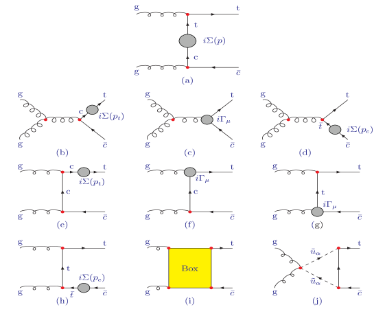
Figure 1: Feynman diagrams for $gg\to t\bar{c}$. Additional diagrams with the two gluons interchanged are not shown.

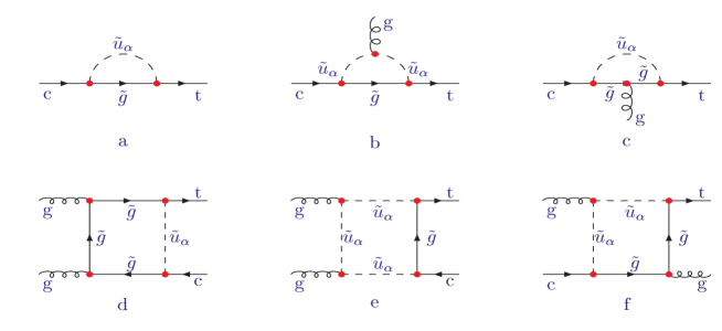
Figure 2: SUSY-QCD contribution to $c-t$ transition, $\bar{t}cg$ interaction and box diagrams for $gg\to t\bar{c}$.

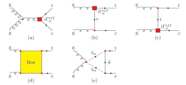
Figure 3: Effective diagrams for the process $gg\to t\bar{c}$. Here $\Gamma^{eff}_{\mu}$ is the effective $\bar{t}cg$ interaction defined in Eq. (36).

Of course, the effective vertex $\bar{t}cg$ is model-dependent since its components $\Gamma_{\mu}^{\bar{t}cg}$ and $\Sigma$ are model-dependent. We obtained their expressions in SUSY QCD analytically. We retain the tensor loop functions rather than expanding them in terms of scalar loop functions as usual Hooft . This method makes our results quite compact and also simplifies our Fortran codes which will be discussed below.

The effective vertex $\bar{t}cg$ in Eq. (36) is a 4-component Lorentz vector and also a $4\times 4$ matrix in Dirac spinor space. In its realization in Fortran coding, we use a dimension-three array $V(i,j,k)$ with $i$ (=1,2,3,4) labeling the Lorentz index and $j,k$ (=1,2,3,4) labeling the spinor indices. We also use arrays to encode other quantities such as Lorentz vectors, Dirac spinors, Lorentz tensors and Dirac $\gamma$ matrices. The steps to calculate the effective interaction in Fortran code can be then summarized as follows:

• Input the matrices $P_{L,R}$, $\gamma^{\mu}P_{L,R}$ and $\sigma^{\mu\nu}$. For any other matrices encountered in the calculation, we use $\gamma$ algebra to generate its elements.

• Use the mass splitting methodBarger to generate events with momentums for the initial and final particles.

• For a generated event with fixed momenta, the components of any tensor loop function can be calculated numerically and stored in arrays.

• Generate the $\gamma$ matrices $\gamma^{\mu_{1}}\cdots\gamma^{\mu_{n}}$ and contract its Lorentz indices with those of tensor loop functions and those of quark momenta to obtain the effective vertex.

To calculate the amplitude of $gg\to t\bar{c}$, we also need to calculate box diagrams. Such calculations are usually tedious if the four-point tensor loop functions are expanded in terms of scalar loop functions. Since we choose to retain the tensor loop functions and contract the indices numerically, our results are quite compact, as shown for $gg\to t\bar{c}$ in the Appendix. The general expression for a box diagram is the sum of fermion chain of the form $\left(\bar{u}\gamma^{\mu_{1}}\cdots\gamma^{\mu_{n}}u\right)\times D_{\mu_{i}\cdots\mu_{j}}\times p_{\mu_{k}}\cdots$ and its numerical value is calculated by the following steps

• Input the wave functions for fermions and define the multiplication of $\gamma$ matrix with the wave function.

• Generate the tensor, say $\bar{u}\cdots\gamma^{\mu_{n-1}}\gamma^{\mu_{n}}u$, and contract its indices with those of loop functions $D_{\mu_{i}\cdots\mu_{j}}$ and those of vectors involved, to get the value of each term in the amplitude.

With the method introduced above, we can also easily calculate other FCNC interactions. Let us take the calculation of $cg\to tZ$ as an example. Its Feynman diagrams can be obtained from Figs. 1-2 by removing those involving triple-gluon interaction and gluon-gluino-gluino interaction, and then replacing any gluon with Z boson. Using the technique from Eq. (35) to introduce the effective $\bar{t}cg$ interaction and the effective $\bar{t}cZ$ interaction, one can again get simplified diagrams similar to Fig. 3(b-e).

Once $gg\to t\bar{c}$ is calculated, evaluation of the others $t\to cg$, $cg\to tg$ and $t\to cgg$ becomes rather easy. The decay $t\to cg$ is now a tree level interaction induced by the interaction $\bar{t}cg$. The amplitudes (or their conjugates) for $cg\to tg$ and $t\to cgg$ are related to that of $gg\to t\bar{c}$, and can be easily obtained by making some simple replacements which can be easily realized in our code.

In the Appendix, we list the explicit forms of all the penguin-induced FCNC interactions discussed in this paper. These interactions are needed to obtain the effective top FCNC interactions.

IV Numerical results and dependence on SUSY parameters

We know, from the discussion in Section II, that the calculations of the SUSY-QCD contributions induced by the flavor mixings between left-handed scharm and stop, depend on the parameters $M_{Q_{2,3}}$, $M_{U_{3}}$, $X_{t}=A_{t}-\mu\cot\beta$, $m_{\tilde{g}}$, $\delta_{LL}$ and $\delta_{LR}$. In this section, we investigate the dependence of the numerical results on these parameters. We first show the results for top quark rare decays. These decay modes occur only via one effective interaction and thus their dependence on the parameters is relatively simple. We perform a comparative study and plot the results for these decays together, to illustrate their dependence on a given set of parameters. After analyzing the features of the top quark rare decays, we extend the study to the FCNC top quark productions. They usually involve two effective interactions and several box diagrams, and thus their dependence on SUSY parameters is more complex.

The SM parameters used in our calculations are pdg

$$m_{t}=172.7{~{}\rm GeV},~{}~{}m_{b}=4.8{~{}\rm GeV},~{}~{}m_{Z}=91.19{~{}\rm GeV},$$

$$\sin\theta_{W}=0.2228,~{}~{}\alpha_{s}(m_{t})=0.1095,~{}~{}\alpha=1/128.$$ (37)

After the assumptions discussed in Sec. III, about 10 SUSY parameters are still involved. We will show below the dependence on SUSY parameters of the top FCNC processes. When one of the parameters is varied, the others will be fixed to their “central” values, taken as

$$M_{\rm SUSY}=M_{Q_{3}}=M_{U_{3}}=M_{Q_{2}}=500{~{}\rm GeV},\quad X_{t}=1000{~{}\rm GeV},\quad m_{\tilde{g}}=250{~{}\rm GeV},\quad\tan\beta=5.$$ (38)

The values of $\delta_{LL}$ and $\delta_{LR}$ will be shown in the figures. With the exception of the last plot in this section (Fig. 12), we adopt the so-called $m_{h}^{\rm max}$ scenario mhmax which is widely discussed in Higgs physics, and which assumes that all the soft mass parameters are degenerate

$$M_{\rm SUSY}=M_{Q_{i}}=M_{U_{i}}=M_{D_{i}},$$ (39)

and that all the trilinear couplings are also degenerate, $A_{u_{i}}=A_{d_{i}}$, with $X_{t}/M_{\rm SUSY}=2$. In investigating the processes $t\to ch$ and $cg\to th$, we used the loop-corrected lightest Higgs boson mass and the effective Higgs mixing anglehollik ; cao . These two quantities involve two additional parameters $\mu$ and $m_{A}$, which are fixed as

$$\mu=m_{A}=500{~{}\rm GeV}.$$ (40)

In our calculations we use CTEQ6L cteq to generate the parton distributions with renormalization scale $\mu_{R}$ and factorization scale $\mu_{F}$, chosen to be $\mu_{R}=\mu_{F}=m_{t}$. To make our predictions more realistic, we applied some kinematic cuts. For example, for the three body decay $t\to cgg$ we require that the energy of each decay product be larger than $15$ GeV and the separation of any two final states be more than $15^{o}$ in the top quark rest frame. For the top quark production channels, we require that the transverse momentum of each produced particle be larger than $15$ GeV and their pseudo rapidity be less than 2.5 in the laboratory frame. Moreover, for $cg\to t$ followed by $t\to bW$, we do not require the top quark exactly on mass shell and instead we require the invariant mass of bottom quark and W boson in a region of $m_{t}-3\Gamma_{t}\leq M_{bW}\leq m_{t}+3\Gamma_{t}$ ($\Gamma_{t}$ is the top quark width). This requirement was once used in Hosch to investigate the observability of this channel at hadron colliders in the effective Lagrangian framework.

Furthermore, we vary the flavor mixings, $\delta_{LL}$ and $\delta_{LR}$, over a wide range, with the only requirement that they satisfy current collider searches for sparticles and Higgs bosonspdg :

$$m_{\tilde{q}}\geq 96{\rm~{}GeV},\quad m_{\tilde{g}}\geq 195{\rm~{}GeV},\quad m_{h}\geq 85{\rm~{}GeV}.$$ (41)

In principle, some low energy data, such as $b-s$ transition and $\delta\rho$, can also constrain these mixings cao . But those so-called indirect constraints are usually quite complicated. To simplify the discussion in this section we do not impose these indirect constraints, but we address such a question in the next section. We checked that the conclusions obtained in this section are valid in the region favored by these indirect constraints .

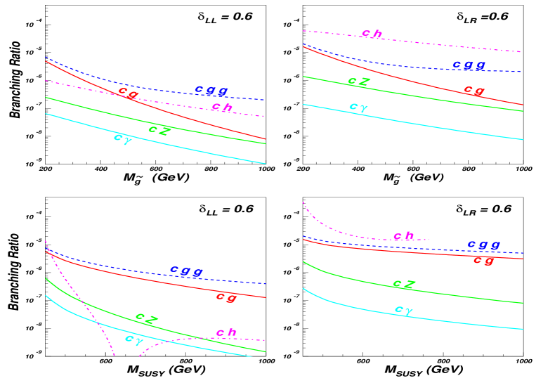
Figure 4: The branching ratios of FCNC top quark decays. Unspecified parameters are given in Eqs. (37-40). The values of $\delta_{LL}$ and $\delta_{LR}$ are arbitrarily chosen, and a smaller value will lower the rates, but not change the tendencies of these curves.

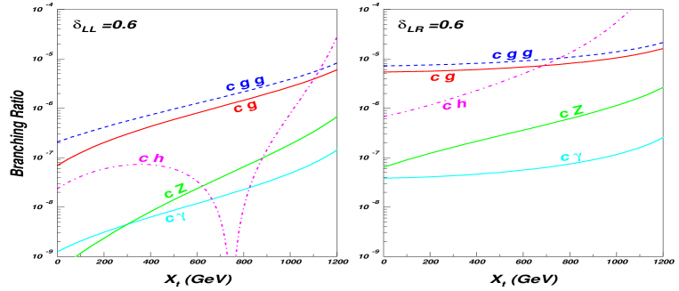
Figure 5: Same as Fig. 4, but as functions of $X_{t}(=A_{t}-\mu\cot\beta)$.

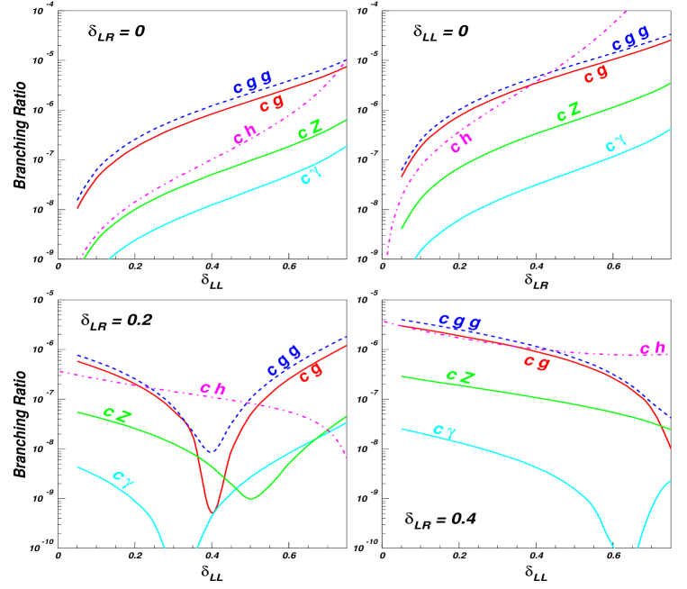
Figure 6: Same as Fig. 4, but as functions of the mixing parameters.

In Figs. 4-6, we present the branching ratios of various FCNC top quark decays, defined with respect to the width $\Gamma_{t}(t\to bW)$ ($\simeq 1.45$ GeV). We plot the six branching ratios for the decays in Eq. (7)-(11) as functions of $m_{\tilde{g}}$, $M_{SUSY}$ and $X_{t}$ in the upper two diagrams of Fig. 4, the lower two diagrams of Fig. 4 and Fig. 5, respectively. We also show the dependence of the branching ratios on the squark mixing parameter $\delta_{LL}$ ($\delta_{LR}$) by fixing the value of $\delta_{LR}$ ($\delta_{LL}$) in Fig. 6. These figures show some common features of all the gauge boson decay modes. The first one is that, as the sparticles become heavy, the branching ratios drops monotonously (see Fig. 4), a reflection of the decoupling property of the MSSM. The second is that, as shown in Fig. 5, the branching ratios increase with the increase of $X_{t}$. This is because $X_{t}$ affects the squark mass splittings and could alleviate the cancellation between different loop contributions. The third feature is that the branching ratios increase rapidly with the flavor mixing $\delta_{LL}$ and $\delta_{LR}$, because the flavor mixings can not only enhance the coupling strength of squark flavor changing interactions, but also enlarge the squark mass splittings. This is illustrated in the first two diagrams of Fig. 6. These last two effects combined make the branching ratios very sensitive to the flavor mixing parameters.

By comparing the case $\delta_{LL}\neq 0$ with the case $\delta_{LR}\neq 0$ throughout Figs. 4-6, one finds that $\delta_{LR}$ induces larger rates with weaker dependence on sparticle masses. Furthermore, when both $\delta_{LL}$ and $\delta_{LR}$ are non-zero, as can be inferred from the last two diagrams of Fig. 6, the $\delta_{LL}$ and the $\delta_{LR}$ dependences interfere destructively. To understand such behaviors, we resort to the mass insertion method, as it can give more intuitive results mass insertion . We take the decay $t\to cg$ as an example. By gauge invariance, the general expression for the effective $\bar{t}cg$ interaction takes the form

$$\Gamma_{\mu}=F_{1}(k^{2})\bar{t}T^{a}(k^{2}\gamma_{\mu}-k_{\mu}\not{\hbox{\kern-2.1pt$k$}})P_{L}cg^{a}-m_{t}F_{2}(k^{2})\bar{t}T^{a}i\sigma_{\mu\nu}k^{\nu}P_{L}cg^{a}$$ (42)

where $F_{1,2}(k^{2})$ are form factors arising from loop calculations. For the decay $t\to cg$, $F_{1}$ does not contribute, since the gluon momentum $k^{\mu}$ satisfies $k^{2}=0$ and $k\cdot\epsilon=0$. So only the dipole moment term is relevant to our discussion. Noting that the dipole changes both the flavor and the chirality of the fermions, we may infer the form of $m_{t}F_{2}$ in the mass insertion approximation. If only $\delta_{LL}$ is considered for flavor changing, $m_{t}F_{2}$ must be

$$m_{t}F_{2}=\frac{m_{t}\delta_{LL}}{M_{SUSY}^{2}}A+\frac{m_{\tilde{g}}\delta_{LL}m_{t}X_{t}}{M_{SUSY}^{4}}B,$$ (43)

where $M_{SUSY}=max(m_{\tilde{g}},M_{\tilde{q}})$, and $A,B$ are dimensionless constants coming from loop functions with $1/M_{SUSY}^{2}$ factored out. The first term corresponds to the top chirality flipping contribution, i.e., obtained by using the relation $\bar{u}_{t}\!\not{\hbox{\kern-4.0pt$p$}}_{t}=m_{t}\bar{u}_{t}$, while the second term corresponds to the $\tilde{t}_{L}-\tilde{t}_{R}$ mixing contribution, and thus associated with the gluino mass. The situation is quite different for $\delta_{LR}\neq 0$, which alone can be responsible for both flavor changing and chirality flipping. In this case, $m_{t}F_{2}$ should be

$$m_{t}F_{2}=\frac{m_{\tilde{g}}\delta_{LR}}{M_{SUSY}^{2}}C.$$ (44)

where $C$, like $A$ and $B$, is a dimensionless constant coming from loop functions with $1/M_{SUSY}^{2}$ factored out. Comparing Eq. (43) with Eq. (44), we find that the latter is larger if $m_{\tilde{g}}\gg m_{t}$. Assuming that $m_{\tilde{g}}\simeq M_{\tilde{q}}$, Eq. (43) scales like $1/M_{SUSY}^{2}$ while Eq. (44) scales like $1/M_{SUSY}$. This explains the fact that $\delta_{LR}$ induces larger rates with weaker dependence on sparticle masses. Moreover, a detailed calculation shows that $m_{t}F_{2}$ in Eq. (43) is of opposite sign to that in Eq. (44), which means that the $\delta_{LL}$ contribution tends to cancel the $\delta_{LR}$ contribution.

The decay $t\to ch$ has similar features to the decay into a gauge boson except for a rather complicated dependence on $M_{SUSY}$ and $X_{t}$, as shown in Figs. 4-5. For the effective $\bar{t}ch$ interaction, with both the top and the charm quarks on-shell, the general expression is

$$\Gamma^{eff}_{\bar{t}ch}=D\bar{t}P_{L}ch,$$ (45)

where $D$ is a form factor emanating from the loop calculation. This interaction, like the effective $\bar{t}cg$ interaction, also involves both flavor change and chirality flip. So in some aspects, the behavior for $t\to ch$ should be similar to $t\to cg$. But its dependence on $X_{t}$ is more complicated than other decay modes. The reason may be that $X_{t}$ not only affects the masses and mixings of squarks, but also affects the Higgs boson mass and its mixing angles, and, further, it enters the interaction of $\tilde{q}^{\ast}\tilde{q}h$.

An interesting feature, shown in Figs. 4-6 is that the branching ratio of $t\to cg$ is always smaller than the higher order decay $t\to cgg$. This was observed in the SM tcgg-sm and the MSSM Gad-pptc-mssm , and it indicates that the QCD corrections to $t\to cg$ may be important. Two reasons may account for this behavior. One is that the QCD factor in the amplitude-square for $t\to cgg$ is much larger than that for $t\to cg$. The other reason is that, unlike the case $t\to cg$, $F_{1}$ in Eq. (42) also contributes to $t\to cgg$ and this contribution is important. From Figs. 4-6, one finds that, in most cases

$$Br(t\to cgg)>Br(t\to cg)>Br(t\to cZ)>Br(t\to c\gamma),$$ (46)

and in some cases $Br(t\to ch)$ may be the largest.

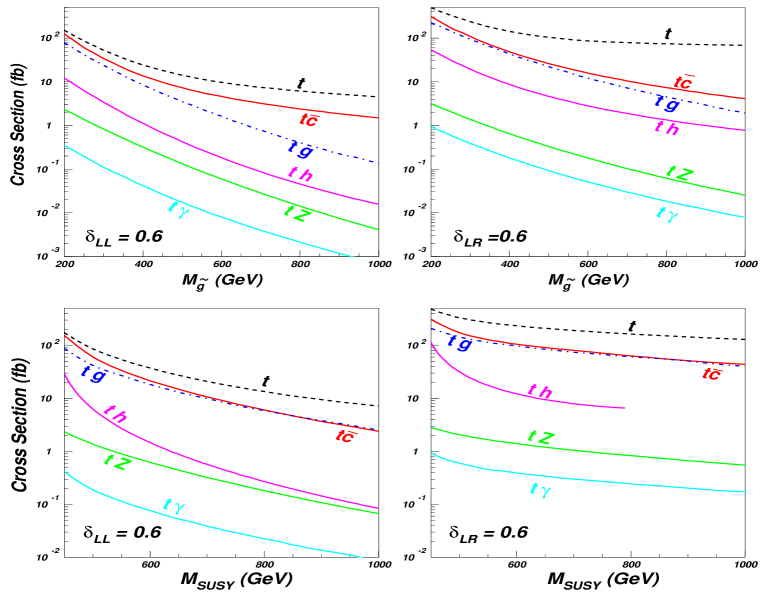
Figure 7: The cross sections of the FCNC top quark productions at the LHC. Each curve labeled by the final states corresponds to a certain production channel.

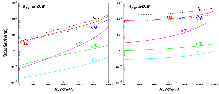
Figure 8: Same as Fig. 7, but as a function of $X_{t}(=A_{t}-\mu\cot\beta)$.

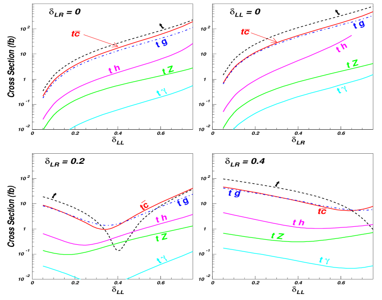
Figure 9: Same as Fig. 7, but as a function of the mixing parameters.

After giving the branching ratios for the FCNC top decays comparatively, we now consider the FCNC top quark production channels. At the LHC the production proceeds through the six parton-level processes shown in Eqs. (1-6), among which only $gg\to t\bar{c}$ has been extensively studied in the MSSMpptc-mssm ; Gad-pptc-mssm . In calculating the cross section for each channel, we also include the rate for its charge conjugate channel. In the following discussions we use the parton process to label its contribution to the hadronic one. Thus, the cross sections mentioned below refer to the hadronic ones.

The dependence of the cross sections on SUSY parameters is plotted in Figs. 7-9. These figures exhibit the same features as the FCNC top quark decays in Fig. 4-6. Thus we do not repeat drawing attention to the same features, and we only point out three remarkable points of these diagrams. The first is that the rate of $cg\to t$ is generally larger than that for $gg\to t\bar{c}$. This is possible because the charm quark in the parton distributions mainly comes from the splitting of a gluon cteq and thus $cg\to t$ can be seen as $gg\to t\bar{c}$ with the final charm quark going along the beam pipe. Analyzing the signal versus background Hosch ; pptc-background , it seems that $cg\to t$ provides a better opportunity for the observation of top production. The second point is that the rate of $cg\to tg$ is comparable to $gg\to t\bar{c}$ in most cases. This coincides with the results in pptc-Han where both modes were studied in the effective Lagrangian approach. Since the two processes have the same signals at colliders, namely single top plus one light-quark jet, one should combine these two when searching for the FCNC top production events. The third point is that in most cases the cross section for $cg\to th$ is one order of magnitude smaller than that for $gg\to t\bar{c}$. The reason is that although $cg\to th$ can proceed either through $\bar{t}cg$ interaction or $\bar{t}ch$ interaction, the two interactions interfere destructively and thus the combined contributions are suppressed.

As shown above, in most of parameter space the rates are expected to be quite small at the LHC. In order to study the observability of such rare processes, it is necessary to scan the whole parameter space to figure out the maximum value that each process can reach. We call the ‘favorable region’ the part of parameter space which gives the maximum value for the rate of an individual channel. Of course, such favorable region is process-dependent. In what follows we take $gg\to t\bar{c}$ as an example to carry out such a parameter scan explicitly. In the next section, the maximal rates for all processes will be tabulated, after discussing the effects of the indirect constraints on the flavor mixing parameters.

In Fig. 10 we plot the maximal cross section for $gg\to t\bar{c}$ as a function of $X_{t}$ with non-zero $\delta_{LL}$ (left panel) and $\delta_{LR}$ (right panel). The maximum value is obtained by fixing $M_{SUSY}$ and $X_{t}$ but varying $m_{\tilde{g}}$ and $\delta_{LL}$ or $\delta_{LR}$. In searching for such maximal values, we required $m_{\tilde{q}}\geq 100$ GeV and $m_{\tilde{g}}\geq 200$ GeV.

For non-zero $\delta_{LL}$, we find that the parameter points for the maximal cross sections correspond to the lightest squark mass and the gluino mass fixed at their allowed lower bound, i.e., 100 GeV and 200 GeV, respectively. This can be easily understood from the decoupling property of the MSSM. At such optimum points, if $M_{SUSY}$ is fixed, $X_{t}$ value is related to $\delta_{LL}$. Since both $X_{t}$ and $\delta_{LL}$ are the off-diagonal elements in squark mass matrix, a large $X_{t}$ will correspond to a small $\delta_{LL}$ and vice versa. Then from Eq. (43), one can see that neither large nor small $X_{t}$ can predict the largest rate for $gg\to t\bar{c}$. This explains the behavior of each curve in the left panel of Fig. 10.

In Fig.  11, we plot the maximal cross section as a function of mixing parameters. For non-zero $\delta_{LL}$ mixings (left panel), we see that the maximal value of each curve lies at a moderate $\delta_{LL}$, which agrees with the above analysis. Among the three curves for different $M_{SUSY}$, the maximal value is obtained for $M_{SUSY}=800$ GeV. The reason is that $M_{SUSY}=800$ GeV implies heavier masses for the other two squarks and alleviates the cancellation between different diagram contributions.

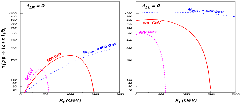
Figure 10: The maximal cross section of $t\bar{c}$ production at the LHC, proceeding through the parton-level channel $gg\to t\bar{c}$, as a function of $X_{t}$ by varying $m_{\tilde{g}}$ and $\delta_{LL}$ or $\delta_{LR}$.

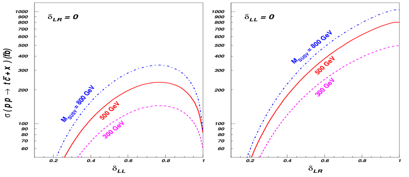
Figure 11: Same as Fig. 10, but as a function of mixing parameters.

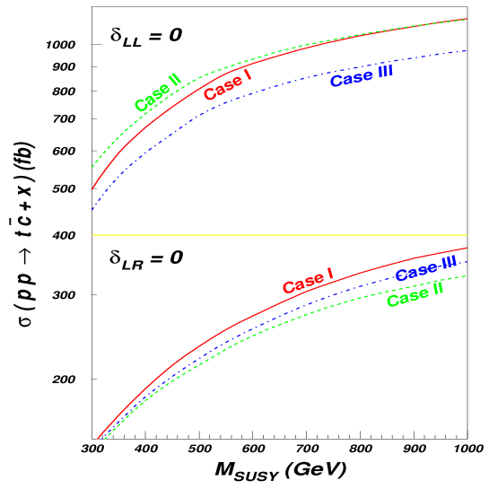
Figure 12: Same as Fig. 10, but as a function of $M_{SUSY}$ under different cases specified in the text.

For the case of non-zero $\delta_{LR}$, maximal cross sections also appear at the lower bounds of the lightest squark mass and the gluino mass. This property together with the effective $\bar{t}cg$ coupling in Eq. (44), imply that the maximal value for each curve should lie at a large $\delta_{LR}$, or by the correlation, at small $X_{t}$. (Both $X_{t}$ and $\delta_{LR}$ appear as the off-diagonal elements in squark mass matrix. Thus, for a given $M_{SUSY}$, their large values enlarge the mass splitting between squark mass eigenstates and lead to a small mass for the lightest squark. Due to the lower bound on the lightest squark mass, $\delta_{LR}$ and $X_{t}$ cannot be both large.) This is in agreement with the behaviors of the curves for non-zero $\delta_{LR}$ shown in the right panels of Figs. 10-11. For the right panel of Fig. 10, we checked that for $M_{SUSY}=800$ GeV, varying $X_{t}$ from 0 to $500$ GeV only resulted in a change of $0.006$ for $\delta_{LR}$. This is the reason that the maximal cross section is insensitive to $X_{t}$ for $X_{t}\leq 500$ GeV.

In Fig. 12 we show the dependence of the maximal cross section on $M_{SUSY}$ for non-zero $\delta_{LL}$ or $\delta_{LR}$ values. To get the maximal cross sections, we fix the lightest squark mass as $100$ GeV and vary the value of $\delta_{LL}$ or $\delta_{LR}$. We considered three cases,

• Case I: $M_{Q_{2}}=M_{Q_{3}}=M_{U_{3}}=M_{SUSY}$,

• Case II: $M_{Q_{3}}=M_{U_{3}}=M_{SUSY}$, $M_{Q_{2}}=1.2M_{SUSY}$,

• Case III: $M_{Q_{3}}=M_{SUSY},M_{U_{3}}=0.8M_{SUSY},M_{Q_{2}}=1.2M_{SUSY}$.

These cases are motivated by mSUGRA model sugra where the three squark masses are generated from the same soft breaking mass parameter $m_{0}$ at supersymmetry breaking scale, but are split due to quark Yukawa couplings when they evolve down to electroweak scale spectrum . From this figure we see that the maximal cross section values increases with $M_{SUSY}$, and for non-zero $\delta_{LL}$ ($\delta_{LR}$), case I (II) gives the largest prediction for the cross sections. These results indicate that in searching for the maximum values of the cross section, we should treat $M_{Q_{2}}$, $M_{Q_{3}}$ and $M_{U_{3}}$ as free parameters and explore all the possibilities for these masses.

Note that in the above discussions we have only considered the case for non-zero $\delta_{LL}$ or $\delta_{LR}$. But as pointed below Eq. (34), most of our conclusions should be valid for the case non-zero $\delta_{RL}$ or $\delta_{RR}\neq 0$ with an interchange of $L$ and $R$.

V Low-energy constraints on FCNC top quark interactions

V.1 Constraints on scharm-stop flavor mixings

We know, from the discussions in the preceding section, that the rates of the FCNC top quark processes depend strongly on the flavor mixing parameters $\delta_{LL}$ and $\delta_{LR}$, which are treated as free. Of course, such a treatment is informative and useful to the LHC experiments since it allows to directly place limits on the mixing parameters once the measurements are made at the LHC.

However, it is worth noting that these mixing parameters may be subject to various direct and indirect experimental constraints. Firstly, since the mixing terms appear as the non-diagonal elements of squark mass matrices, they can affect the squark mass spectrum, especially by enlarging the mass splitting between squarks. Therefore they should be constrained by the squark mass bounds from the direct experimental searches. At the same time, since the squark loops affect the precision electroweak quantities such as $M_{W}$ and the effective weak mixing angle $\sin^{2}\theta_{eff}$hollik ; mw-mssm , such mixings could also be constrained by precision electroweak measurements. As shown inhollik ; cao , to a good approximation, the supersymmetric corrections to the electroweak quantities contribute through the $\delta\rho$ parameter and thus sensitive to the mass splitting of squarks. Secondly, the processes governed by $b\to s$ transition like $B_{s}-\bar{B}_{s}$ mixings Ball and $b\to s\gamma$bsr can provide rich information about the $\tilde{s}-\tilde{b}$ mixings. Through the SU(2) relation between the up-squark and down-squark mass matrices (see Eq. (29)) and also through the electroweak quantities (since all squarks contribute to electroweak quantities via loops), the information can be reflected in the up-squark sector and hence constrain the scharm-stop mixings. Thirdly, we note that the chiral flipping mixings of scharm-stop come from the trilinear $H_{2}\tilde{c}_{L}^{\ast}\tilde{t}_{R}$ interactionssusyflavor . Such interactions can lower the lightest Higgs boson mass $m_{h}$ via squark loops and thus should be subject to the current experimental bound on $m_{h}$.

In cao these constraints were examined and it was shown that, although they usually depend on additional unknown parameters in the down-type squark mass matrix, a combined analysis can still severely restrict the mixings $\delta_{LL}$ and $\delta_{LR}$ in most cases. Here we extend the analysis of cao by providing more examples about these constraints and then perform a detailed investigation of the maximum rates for various top quark FCNC processes both with and without these constraints.

The constraints considered in our paper are $b\to s\gamma$, $B_{s}-\bar{B}_{s}$ mixing, $\delta M_{W}$ and $\delta\sin^{2}\theta_{eff}$ and the lightest Higgs boson mass. In the following, we first recapitulate these constraints and then apply them to scharm-stop mixings.

• $b\to s\gamma$: In the MSSM, there are four kinds of loops contributing to $b\to s\gamma$ mediated respectively by the charged Higgs bosons, charginos, neutralinos and gluinos, each of which may be sizable bsr . For a light charged Higgs mass, the contribution from the charged Higgs is quite large and always has the same sign as the SM contribution, and thus enhance the branching ratio to very high values charged higgs . The current $b\to s\gamma$ data require either a sufficiently heavy charged Higgs boson, or its contribution should be canceled by other parts of SUSY effects. For the other three kinds of contributions, depending on SUSY parameters, they may interfere constructively or destructively with the SM effects and thus their relative sizes are not fixed bsr-character . The effect of these properties of SUSY on $b\to s\gamma$ makes it necessary to consider all the contributions simultaneously in discussing $b\to s\gamma$ constraints on the squark flavor mixing parameters.

  Current measurement of the branching ratio for $b\to s\gamma$ is rather precise, with $3\sigma$ bounds given by heavy flavor

  $$2.53\times 10^{-4}<Br(b\to s\gamma)<4.34\times 10^{-4}.$$ (47)

  With the SM prediction $Br^{NLO}(b\to s\gamma)=(3.53\pm 0.30)\times 10^{-4}$ bsr-sm and a favored negative $C_{7}$ by $b\to sl^{+}l^{-}$ bsll , where $C_{7}$ denotes the Wilson coefficient for the electromagnetic dipole operator ${\cal O}_{7}$, this decay can severely restrict the SUSY parameters. Our numerical results indicate that it is very sensitive to $\delta^{d}_{LR}$ and $\delta^{d}_{RL}$ for most cases, and for large $\tan\beta$, it is sensitive to $\delta_{LL}$ as well. The same results also indicate that $b\to s\gamma$ depends weakly on $\delta_{LR}$ which affects the decay via chargino-mediated loops, but under all circumstances $b\to s\gamma$ is not sensitive to $\delta_{RL}$ and $\delta_{RR}$.

• $B_{s}-\bar{B}_{s}$ mixing: In the MSSM, although the loops mediated by charged Higgs boson, chargino and neutralino contribute to $B_{s}-\bar{B}_{s}$ mixing, their effects are generally much smaller than the SM contributionBall . So when discussing the constraint of $B_{s}-\bar{B}_{s}$ mixing on squark flavor mixing parameters, we only consider gluino contributions. Recently, the D0 collaboration gave the first two-side bound on the mass splitting between $B_{s}$ and $\bar{B}_{s}$ Abazov:2006dm

  $$17~{}{\rm ps}^{-1}<\Delta M_{s}<21~{}{\rm ps}^{-1}\quad(90\%~{}{\rm C.L.})$$ (48)

  This result is in agreement with the SM prediction, which is estimated as $21.3\pm 2.6~{}{\rm ps}^{-1}$ by the UTfit group Bona:2005vz and $20.9^{+4.5}_{-4.2}~{}{\rm ps}^{-1}$ by the CKMfitter group Charles:2004jd . After considering various uncertainties, the bounds in Eq. (48) can be re-expressed asEndo:2006dm

  $$0.55<|1+M_{12}^{SUSY}/M_{12}^{SM}|<1.37,$$ (49)

  where $M_{12}$ is the transition matrix element for $B_{s}-\bar{B}_{s}$ transition. As pointed out inBall , $B_{s}-\bar{B}_{s}$ mixing is very sensitive to the combinations $\delta_{LL}\delta_{RR}^{d}$ and $\delta_{LR}^{d}\delta_{RL}^{d}$ and thus can put rather stringent constraints on any of $\delta^{d}$s.

• $\delta M_{W}$ and $\delta\sin^{2}\theta_{eff}$: In the MSSM, the corrections to $M_{W}$ and $\sin^{2}\theta_{eff}$ involve the calculation of the gauge boson self energy, and among all kinds of contribution to the self energy, those from squark loops are most importantrho . As a good approximation, $\delta M_{W}$ and $\delta\sin^{2}\theta_{eff}$ are related to $\delta\rho$ byhollik

  $$\delta M_{W}\simeq\frac{M_{W}}{2}\frac{c_{W}^{2}}{c_{W}^{2}-s_{W}^{2}}\delta\rho,$$

  $$\delta\sin^{2}\theta_{eff}\simeq-\frac{c_{W}^{2}s_{W}^{2}}{c_{W}^{2}-s_{W}^{2}}\delta\rho,$$ (50)

  where

  $$\delta\rho\equiv\frac{\Sigma_{Z}(0)}{M_{Z}^{2}}-\frac{\Sigma_{W}(0)}{M_{W}^{2}}.$$ (51)

  Since the couplings are stronger for left-handed squarks than for right-handed squarks, $\delta\rho$ is sensitive to the mass splittings between left-handed up-squarks and down-squarks rho . As far as $\delta_{LL}$ is concerned, due to the $SU(2)$ relation in Eq. (29), it changes up-squark and down-squark mass spectra simultaneously and thus its effects on $\delta\rho$ are generally small even for large $\delta_{LL}$. For $\delta_{LR}$ and $\delta_{RL}$, they are independent of $\delta_{LR}^{d}$ and $\delta_{RL}^{d}$, which are very small as required by $b-s$ transition bsr ; Ball ; B-summary . Thus a large $\delta_{LR}$ or $\delta_{RL}$ can induce a sizable mismatch between up-squark and down-squark mass spectra. As a result, large $\delta_{LR}$ or $\delta_{RL}$ can significantly change $\delta\rho$ cao .

  With the recent analysis of the LEP data, the uncertainties in measuring $M_{W}$ and $\sin^{2}\theta_{eff}$ were significantly lowered to read lep

  $$\delta M_{W}<34{\rm~{}MeV},\quad\delta\sin^{2}\theta_{eff}<15\times 10^{-5}.$$ (52)

  These uncertainties imply that the new physics influence on $\delta\rho$ should be lower than $5.5\times 10^{-4}$.

• Higgs boson mass $m_{h}$: In the MSSM the loop-corrected lightest Higgs boson mass $m_{h}$ is defined as the pole of the corrected propagator matrix, which can be obtained by solving the equation Dabelstein

  $$\left[p^{2}-m_{h,tree}^{2}+\hat{\Sigma}_{hh}(p^{2})\right]\left[p^{2}-m_{H,tree}^{2}+\hat{\Sigma}_{HH}(p^{2})\right]-\left[\hat{\Sigma}_{hH}(p^{2})\right]^{2}=0,$$ (53)

  where $m_{h,tree}$ and $m_{H,tree}$ are the tree-level masses of the neutral Higgs bosons $h$ and $H$, and $\hat{\Sigma}_{i}(p^{2})$ ($i=hh$, $hH$, $HH$) are the renormalized Higgs boson self energies. Among all SUSY contributions to the Higgs boson self energies, those from top and stop loops are by far dominant because of the large top quark Yukawa couplingsh-original . In the presence of the flavor mixings in the up-squark mass matrix, stops will mix with other squarks, and in this case, the dominant contribution comes from the up-squark sector hollik ; feynhiggs .

  Our results indicate that the Higgs boson mass is more sensitive to $\delta_{LR}$ than to $\delta_{LL}$. The reason is that $\delta_{LL}$ affects the Higgs boson mass only by changing the squark interaction through the unitary matrix $\Gamma$ in Eq. (30) while $\delta_{LR}$ can also appear directly in the coupling of trilinear $H_{2}\tilde{c}_{L}\tilde{t}_{R}$ interaction, since the $\delta_{LR}M_{Q_{2}}M_{U_{3}}$ term in up-squark mass matrix comes from this trilinear interaction, and this can reduce the lightest Higgs boson mass. Current collider searches for a MSSM Higgs boson have given the lower bounds on $m_{h}$ in five benchmark scenarios in Higgs physicsbenchmark . In our calculation, we use the limit

  $$m_{h}>\left\{\begin{array}[]{ll}92.8{~{}\rm GeV}&\quad{~{}\rm for}\ m_{h}^{max}\ {~{}\rm scenario}\\ &\\ 85{~{}\rm GeV}&\quad{~{}\rm for~{}other~{}scenarios}\end{array}\right.$$ (57)

As the first example of these constraints, we consider the $m_{h}^{max}$ scenario with the parameters given in Eqs. (38,40). To determine these constraints, we also need to specify the values of the parameters in the down-squark mass matrix and the gaugino mass $M_{2}$. In Fig. 13 we show the allowed region in $\delta_{LL}-\delta_{LR}$ plane for the parameters

$$M_{S}=M_{Q_{i}}=M_{U_{i}}=M_{D_{i}}=500{~{}\rm GeV},~{}~{}X_{t}1000{~{}\rm GeV},~{}~{}M_{\tilde{g}}=250{~{}\rm GeV},~{}~{}\tan\beta=5,$$

$$\mu=M_{A}=M_{2}=500{~{}\rm GeV},~{}~{}\delta_{RL}=\delta_{RR}0,~{}~{}\delta^{d}_{LR}=\delta^{d}_{RL}=\delta^{d}_{RR}=0.$$ (58)

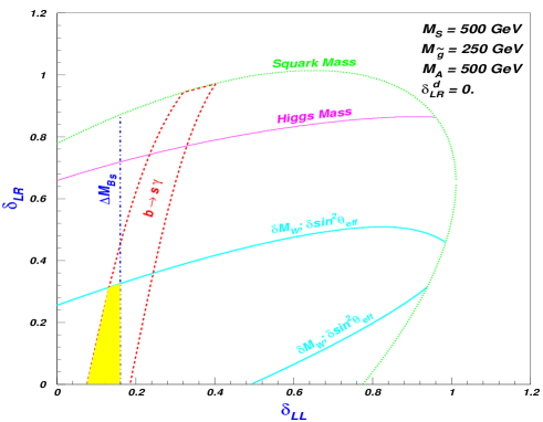
Figure 13: Experimental constraints on $\delta_{LL}$ versus $\delta_{LR}$ with the parameters given in Eq. (58). The region under or left to each curve corresponds to the allowed region. The dashed-line enclosed area is allowed by $b\to s\gamma$. The colored area is the overlap region satisfying all the constraints.

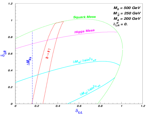
Figure 14: Same as Fig. 13, but for $M_{A}=200$ GeV.

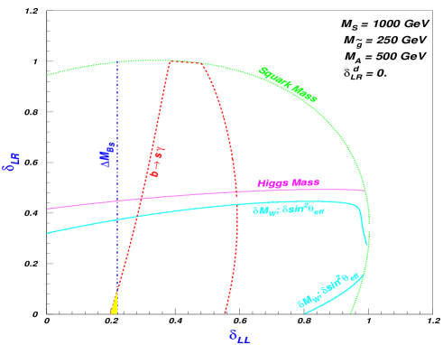
Figure 15: Same as Fig. 13, but for $M_{S}=1$ TeV.

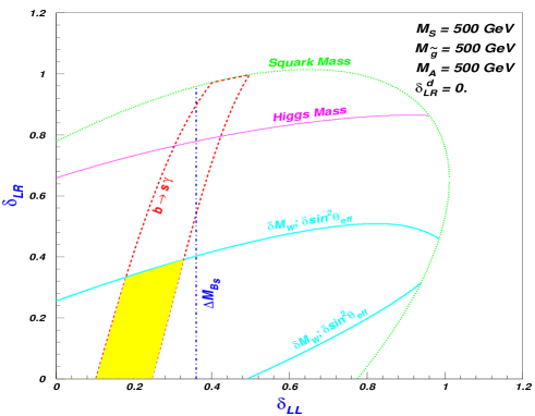
Figure 16: Same as Fig. 13, but for $M_{\tilde{g}}=500$ GeV.

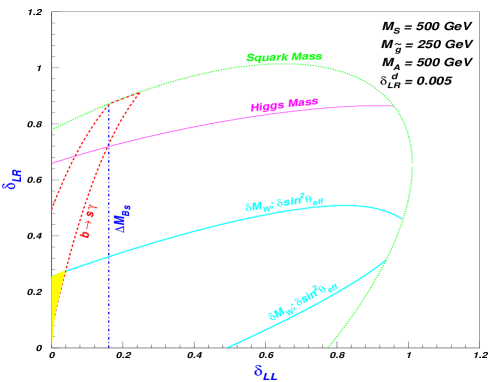
Figure 17: Same as Fig. 13, but for $\delta^{d}_{LR}=0.005$.

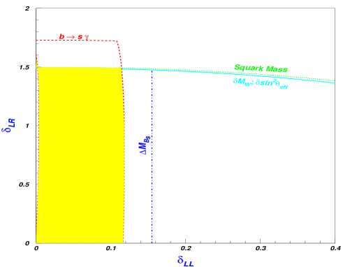
Figure 18: Same as Fig. 13, but for the parameters in Eq. (59). In this case the Higgs boson mass cannot impose any constraints.

Each curve in this figure corresponds to an experimental bound from Eqs. (41), (47), (49), (52) and (57); while the colored area is the overlap region satisfying all the constraints. The distinctive character of this figure is that $b\to s\gamma$ requires a non-zero $\delta_{LL}$. The reason is that with the fixed parameters in Eq. (58), especially with $\delta^{d}_{LR}=0$, the charged Higgs contribution enhances the SM contribution and, as a result, a none-zero gluino contribution is needed to cancel such effects. From Fig. 13 we see that the allowed region is mainly determined by $b\to s\gamma$ and $B_{s}-\bar{B}_{s}$ mixing. To show the dependence of such allowed region on SUSY parameters, we vary the values of $M_{A}$, $M_{S}$, $M_{\tilde{g}}$ and $\delta_{LR}^{d}$ one at a time, and get the allowed region (colored area) in Figs. 14, 15, 16 and 17, respectively. Explicitly, Fig. 14 corresponds to the parameters in Eq. (58) but with $M_{A}=200$ GeV, Fig. 15 corresponds to the parameters in Eq. (58) but with $M_{S}=1000$ GeV , and Fig. 16 and Fig. 17 are drawn in a similar way. The shift of the allowed region can be well understood by the properties of each constraint. Take Fig. 14 as an example. As $M_{A}$ becomes smaller, the charged Higgs contribution to $b\to s\gamma$ further enhance the SM contribution and consequently a larger $\delta_{LL}$ is needed to cancel such effect and satisfy the bound in Eq. (47). Since the constraint from $B_{s}-\bar{B}_{s}$ mixing is not changed, the overlap region diminishes gradually and finally vanishes for $M_{A}\simeq 200$ GeV.

As the second example, we consider the following parameters as an input

$$M_{Q_{2}}=400{\rm~{}GeV},\quad M_{Q_{3}}=1000{\rm~{}GeV},\quad M_{U_{3}}=120{\rm~{}GeV},\quad M_{\tilde{g}}=196{\rm~{}GeV},\quad M_{A}=160{\rm~{}GeV},$$

$$X_{t}=33{\rm~{}GeV},\quad\mu=-330{\rm~{}GeV},\quad M_{2}=860{\rm~{}GeV},\quad M_{D_{i}}=M_{Q_{1}}=M_{D_{1}}=500{\rm~{}GeV},$$

$$\delta_{LR}^{d}=0.0026,\quad\delta_{RL}=\delta_{LR}=0,\quad\delta_{RL}^{d}=\delta_{RR}^{d}=0.$$ (59)

This set corresponds to a point in the parameter space where $cg\to t$ is maximized for non-zero $\delta_{LR}$ (see following discussion about Table 1 and Table 2) and the results are depicted in Fig. 18. Since the squark masses are not universal, $\delta_{LR}>1$ can still satisfy all the constraints and thus is allowed. The reason for this is that all the constraints actually limit the size of the product $\delta_{LR}M_{Q_{2}}M_{U_{3}}$. For the case discussed here, $M_{Q_{2}}$ and $M_{U_{3}}$ are not large and thus a large $\delta_{LR}$ is allowed.

A common property of the above several figures is that $B_{s}-\bar{B}_{s}$ mixing and $b\to s\gamma$ require a small $\delta_{LL}$ value. This is a general feature, which accounts for the significant suppression of the maximal predictions for various top quark FCNC interactions after considering all the constraints (see the results in case I($\delta_{LR}=0$) of Table 1) . We also considered the constraints on $\delta_{RL}$ and $\delta_{RR}$, which, as we pointed out earlier in this section, do not significantly affect $b\to s\gamma$ and $B_{s}-\bar{B}_{s}$ mixing, and hence are constrained only by $\delta\rho$ and the Higgs boson mass. We found that by comparing with the constraints on $\delta_{LR}$ and $\delta_{LL}$, the constraints on these two mixing parameters, especially on $\delta_{RR}$, are rather weak. Let us consider parameters in Eq. (58) as an example. For $\delta_{LL}=\delta_{LR}=0$, our results indicate that $\delta_{RR}$ and $\delta_{RL}$ should be less than $0.76$ and $0.46$, respectively. Such constraints come from $\delta M_{W}$ and $\delta\sin^{2}\theta_{eff}$, and are sensitive to $X_{t}$. For $X_{t}=0$, the bounds will be relaxed to $0.98$ for $\delta_{RR}$ and $0.75$ for $\delta_{RL}$.

V.2 Maximal predictions in MSSM for FCNC top quark processes

With the constraints discussed above, we perform a scan over the SUSY parameter space to search for the maximal predictions of the MSSM on various top quark FCNC processes. We consider two cases: (I) only $\delta_{LL}\neq 0$ and (II) only $\delta_{LR}\neq 0$. For each case, we require the parameters to vary in the following ranges

$$2<\tan\beta<60,\quad\quad\quad\quad\quad\quad 0<M_{Q_{i},U_{i},D_{i}}<1{\rm~{}TeV},$$

$$94{\rm~{}GeV}<m_{A}<1{\rm~{}TeV},\quad\quad 195{\rm~{}GeV}<m_{\tilde{g}}<1{\rm~{}TeV},$$

$$0<\delta_{LL}\ or\ \delta_{LR}<2,\quad\quad\quad\quad-1{\rm~{}TeV}<\mu,M_{2}<1{\rm~{}TeV},$$

$$0<\delta_{LR}^{b}<0.1,\quad\quad\quad\quad\quad\quad\;-2{\rm~{}TeV}<A_{t,b}<2{\rm~{}TeV}.$$ (60)

To manifest the effect of the combined constraints on the maximal rates, we present two types of predictions: one by only requiring the squark, chargino and neutralino masses satisfy their current lower bounds

$$m_{\tilde{u}}>96{\rm~{}GeV},\quad m_{\tilde{d}}>89{\rm~{}GeV},\quad m_{\tilde{\chi}^{0}}>46{\rm~{}GeV},\quad m_{\tilde{\chi}^{+}}>94{\rm~{}GeV};$$ (61)

and the other by imposing all constraints in Eqs. (61, 47, 49, 52, 57). With five million samples for each process in either case, we obtain the maximal predictions and they are given in Table I. From the table one can see that the combined constraints can significantly decrease the MSSM predictions for top-quark FCNC channels at the LHC, especially for the case I, and among these FCNC processes, $cg\to th$ is the most affected one after imposing these constraints. The reason is that, as we pointed out before, there is a cancellation between the contribution from the effective interactions $\bar{t}cg$ and $\bar{t}ch$, and the constraints only allow a region with strong cancellation.

Table 1: Maximal predictions for top-quark FCNC processes induced by stop-scharm mixings via gluino-squark loops in the MSSM. For the production channels we show the hadronic cross sections at the LHC obtained from the given parton-level channels and the corresponding charge-conjugate channels. For the decays we show the branching ratios. LHC sensitivities listed in the last column are for 100fb^-1 integrated luminosity.

	$\delta_{LL}\neq 0$		$\delta_{LR}\neq 0$		LHC sensitivity
	constraints	constraints	constraints	constraints	at $3\sigma$ level
	masses	all	masses	all
$t\to ch$	$1.2\times 10^{-3}$	$2.0\times 10^{-5}$	$2.5\times 10^{-2}$	$6.0\times 10^{-5}$	$5.8\times 10^{-5}$ tch-Aguilar
$t\to cg$	$5.0\times 10^{-5}$	$5.0\times 10^{-6}$	$1.3\times 10^{-4}$	$3.2\times 10^{-5}$	$-$
$t\to cgg$	$6.1\times 10^{-5}$	$7.1\times 10^{-6}$	$1.5\times 10^{-4}$	$3.5\times 10^{-5}$	$-$
$t\to cZ$	$5.0\times 10^{-6}$	$5.7\times 10^{-7}$	$1.2\times 10^{-5}$	$1.8\times 10^{-6}$	$3.6\times 10^{-5}$ tcz-Han ; tcz-Atlas
$t\to c\gamma$	$9.0\times 10^{-7}$	$1.5\times 10^{-7}$	$1.3\times 10^{-6}$	$5.2\times 10^{-7}$	$1.2\times 10^{-5}$ tcr-Han ; tcr-Beneke
$cg\to t$	1450 fb	225 fb	3850 fb	950 fb	800 fbHosch
$gg\to t\bar{c}$	1400 fb	240 fb	2650 fb	700 fb	1500 fb pptc-Han ; pptc-background
$cg\to tg$	800 fb	85 fb	1750 fb	520 fb	1500 fb pptc-Han ; pptc-background
$cg\to t\gamma$	4 fb	0.4 fb	8 fb	1.8 fb	5 fb zt-Aguilar
$cg\to tZ$	11 fb	1.5 fb	17 fb	5.7 fb	35 fb zt-Aguilar
$cg\to th$	550 fb	18 fb	12000 fb	24 fb	200 fb tch-Aguilar

Table 2: SUSY parameters leading to the maximal predictions for $\delta_{LR}\neq 0$ in Table 1.

process	$M_{Q_{2}}(GeV)$	$M_{Q_{3}}(GeV)$	$M_{U_{3}}(GeV)$	$X_{t}(GeV)$	$m_{\tilde{g}}(GeV)$	$\delta_{LR}$
$t\to ch$	1000	900	225	500	195	1.1
$t\to cg$	310	985	90	100	195	1.72
$t\to cgg$	310	980	90	35	195	1.75
$t\to cZ$	500	900	165	600	198	1.1
$t\to c\gamma$	290	1000	90	20	196	1.72
$cg\to t$	400	990	120	33	196	1.5
$gg\to t\bar{c}$	310	990	85	80	196	1.8
$cg\to tg$	490	900	125	0	197	1.45
$cg\to t\gamma$	280	1000	85	25	197	1.78
$cg\to tZ$	370	920	80	115	196	1.86
$cg\to th$	280	1000	85	23	197	1.77

As one can see from Table 1, predictions for the case with non-zero $\delta_{LR}$ are larger than for the one with non-zero $\delta_{LL}$. In Table 2 we list the SUSY parameters leading to the maximal predictions in Table 1 for the case II ($\delta_{LR}\neq 0$). It is seen from Table 2 that the ‘favorable’ parameters for the maximal rates are process dependent. Since these parameters could be first tested by seeking top quark FCNC signals at LHC, in Table 3 we present the predictions for all processes with two sets of parameters, called ‘Point 1’ and ‘Point 2’, where $t\to ch$ and $cg\to t$ are required to be maximized, respectively. It is seen that ‘Point 1’ favors $cg\to t$ as the production channel but ‘Point 2’ favors $t\to cgg$ among the decay modes.

Note that in Table 1 we only showed the cases of $\delta_{LL}\neq 0$ and $\delta_{LR}\neq 0$. For $\delta_{RL}\neq 0$, we found that the maximal rate of $t\to cg$ is $1.3\times 10^{-4}$ if only the squark mass constraints are included and $6\times 10^{-5}$ with all the constraints. For $\delta_{RR}\neq 0$, the maximal rate of $t\to cg$ is $5.0\times 10^{-5}$ with only the squark mass constraints and $4.85\times 10^{-5}$ with all the constraints. These results can be easily understood since, as discussed in cao and in this section, the constraints on $\delta_{RL}$ and $\delta_{RR}$ are weaker than those for $\delta_{LR}$ and $\delta_{RR}$, respectively.

Table 3: SUSY predictions for the rates of top quark FCNC processes at two points of parameter space: ‘Point 1’ maximizes $t\to ch$ and ‘Point 2’ maximizes $cg\to t$ channel.

process	Point 1	Point 2
$t\to cg$	$2.0\times 10^{-5}$	$3.1\times 10^{-5}$
$t\to cgg$	$2.9\times 10^{-5}$	$3.5\times 10^{-5}$
$t\to cZ$	$1.4\times 10^{-6}$	$1.2\times 10^{-6}$
$t\to c\gamma$	$2.6\times 10^{-7}$	$5.2\times 10^{-7}$
$t\to ch$	$6.0\times 10^{-5}$	$7.0\times 10^{-9}$
$cg\to t$	660 fb	950 fb
$gg\to t\bar{c}$	450 fb	690 fb
$cg\to tg$	280 fb	415 fb
$cg\to tZ$	2.3 fb	4.9 fb
$cg\to t\gamma$	1.2 fb	1.8 fb
$cg\to th$	24 fb	8.5 fb

V.3 Top FCNC observability at the LHC

Now we consider the observability of these top quark FCNC interactions at the LHC. This issue has been intensively investigated in the effective Lagrangian approach for $t\to ch$ tch-Aguilar , $t\to cZ$ tcz-Han ; tcz-Atlas , $t\to c\gamma$ tcr-Han ; tcr-Beneke , $pp\to t+X$ Hosch , $pp\to t\bar{c}+X$ pptc-Han ; pptc-background , $pp\to tg+X$pptc-Han ; pptc-background , $pp\to tZ+X$zt-Aguilar , $pp\to t\gamma+X$zt-Aguilar and $pp\to th+X$tch-Aguilar . At the LHC, most of the top quarks will be pair-produced. One of the tops is assumed to subsequently decay as $t\to bW$ (normal mode) while the other top goes to one of the above channels via FCNC interactions (exotic mode).

Due to the large QCD backgrounds at the LHC, the search for these processes must be performed in the decay channels $W\to\ell\bar{\nu}_{\ell}$ ($\ell=e,\mu$) for $W$ boson, $Z\to\ell^{+}\ell^{-}$ for $Z$ boson and $h\to b\bar{b}$ for Higgs boson. For any of these reactions, top quark reconstruction is required to extract the signal from its background. In Table 4, we list the signals and the main backgrounds. The detailed Monte Carlo simulations for the signals and backgrounds can be found in the corresponding literature listed in the last column of Table 1, where the LHC sensitivity for these processes is quoted. Although these sensitivities are based on the effective Lagrangian approach and may be not perfectly applicable to the MSSM, we can take them as a rough criteria to estimate the observability of these channels. Comparing these sensitivities with the SUSY predictions, one can see that only the maximal predictions for $cg\to t$ and $t\to ch$ are slightly larger than the corresponding LHC sensitivities. This implies that the study of these processes may provide the first insight about top quark FCNC. From these sensitivities one can also see that, although the $gg\to t\bar{c}$ channel is now the most extensively studied among the FCNC production channels pptc-mssm , its observation needs a higher luminosity. This is because $gg\to t\bar{c}$ has large irreducible backgrounds from single top productions in the SM pptc-background . Note that in Table 1, we did not list the sensitivity of the LHC to $t\to cg$, which has not been investigated because of a general belief that this decay is not well suited for detecting $\bar{t}cg$ interaction Aguilar-Saavedra:2004wm . In fact, this decay was once investigated for the Tevatron tcg-Han , and it was found that due to the large background, namely $W$ boson plus three jets, only a branching ratio as large as $5\times 10^{-3}$ may be accessible with 10 fb^-1 integrated luminosity. This rate is about one order larger than that for $t\to c\gamma$ at the Tevatron with the same luminosity tcr-Han . For the decay $t\to cgg$, there is an additional jet in its signal and its observability needs to be studied by a detailed Monte Carlo simulation.

Table 4: Experimental signature and main background for FCNC top rare decays and productions at the LHC. The top quarks are assumed to decay $t\to W^{+}b\to\ell^{+}\nu_{\ell}b$, and $Z$ and $h$ bosons decay in the channel $Z\to\ell^{+}\ell^{-}$ and $h\to b\bar{b}$, respectively.

Process	Signal	Background		Process	Signal	Background
$t\bar{t}$, $t\to cg$	$jj\ell\nu b$	$Wjjj$		$cg\to t$	$\ell\nu b$	$Wj$
$t\bar{t}$, $t\to cgg$	$jjj\ell\nu b$	$Wjjjj$		$gg\to t\bar{c}$	$\ell\nu bj$	$tj$
				$cg\to tg$	$\ell\nu bj$	$tj$
$t\bar{t}$, $t\to cZ$	$\ell^{+}\ell^{-}j\ell\nu b$	$ZWjj$		$cg\to tZ$	$\ell^{+}\ell^{-}\ell\nu b$	$ZWj$
$t\bar{t}$, $t\to c\gamma$	$\gamma j\ell\nu b$	$\gamma Wjj$		$cg\to t\gamma$	$\gamma\ell\nu b$	$\gamma Wj$
$t\bar{t}$, $t\to ch$	$b\bar{b}j\ell\nu b$	$Wb\bar{b}jj$		$cg\to th$	$b\bar{b}\ell\nu b$	$t\bar{t}$

VI Conclusions

In this paper, we investigated systematically the SUSY-induced top quark FCNC processes at the LHC, which includes various decay modes and production channels. We performed a comparative study for all the decay modes and for all the production channels so that one can see clearly which decay mode or production channel can have a relatively large rate. The dependence of these channels on the relevant SUSY parameters is investigated in detail and its properties are analyzed. We note that such a global study of the top quark FCNC processes has been done only in a model independent way Aguilar-Saavedra:2004wm . We also analyzed the characteristics of the ‘favorable region’ in SUSY parameter space where the FCNC processes are maximized. After getting an understanding of these processes, we examined the effects of all the direct and indirect experimental constraints on the scharm-stop flavor mixings and scanned the parameter space to find their maximal rates with these constraints imposed. We found that $cg\to t$ and $t\to ch$ are the most likely channels to be observable at the LHC if the MSSM is the correct scenario beyond the SM.

Appendix A Expressions for the Loop results

If significant flavor mixings exist only between left-handed scharm with stops, the squark states $\tilde{c}_{L}$, $\tilde{t}_{L}$ and $\tilde{t}_{R}$ will mix together to induce various top quark FCNCs. In this case, other squark states only serve as spectators to the processes considered in this paper. So in the actual calculation, we only need to consider the squark mass matrix for $(\tilde{t}_{L},\tilde{t}_{R},\tilde{c}_{L})$, which is given by

$$\left(\begin{array}[]{ccc}M_{Q_{3}}^{2}+m_{t}^{2}+(\frac{1}{2}-\frac{2}{3}s_{W}^{2})m_{Z}^{2}\cos 2\beta&m_{t}(A_{t}-\mu\cot\beta)&\delta_{LL}M_{Q_{2}}M_{Q_{3}}\\ m_{t}(A_{t}-\mu\cot\beta)&M_{U_{3}}^{2}+m_{t}^{2}+\frac{2}{3}s_{W}^{2}\cos 2\beta&\delta_{LR}M_{Q_{2}}M_{U_{3}}\\ \delta_{LL}M_{Q_{2}}M_{Q_{3}}&\delta_{LR}M_{Q_{2}}M_{U_{3}}&M_{Q_{3}}^{2}+(\frac{1}{2}-\frac{2}{3}s_{W}^{2})m_{Z}^{2}\cos 2\beta\end{array}\right).$$ (65)

This mass matrix can be diagonalized by a unitary matrix $V$, and it enters the squark interactions as in Eq. (30).

In this Appendix, we list the expressions for $\Sigma$ and $\Gamma^{\bar{t}cg}_{\mu}$ in Eq. (36) which are needed to get the effective $\bar{t}cg$ vertex. We also list the expressions for $\Gamma^{\bar{t}c\gamma}$, $\Gamma^{\bar{t}cZ}$ and $\Gamma^{\bar{t}ch}$ to calculate other effective vertices. Before presenting these expressions, we define the following abbreviations:

$$R^{a} = \sum_{\lambda=1}^{3}V_{1\lambda}V_{\lambda 3}^{\dagger}B(p,m_{\tilde{g}},m_{\lambda}),\quad R^{b}=R^{a}|_{V_{1\lambda}\to V_{2\lambda}},$$ (66)

$$R^{c} = \sum_{\lambda=1}^{3}V_{1\lambda}V_{\lambda 3}^{\dagger}C(-p_{c},p_{c}-p_{t},m_{\tilde{g}},m_{\lambda},m_{\lambda}),\quad R^{d}=R^{c}|_{V_{1\lambda}\to V_{2\lambda}},$$ (67)

$$R^{e} = \sum_{\lambda=1}^{3}V_{1\lambda}V_{\lambda 3}^{\dagger}C(-p_{c},p_{c}-p_{t},m_{\lambda},m_{\tilde{g}},m_{\tilde{g}}),\quad R^{f}=R^{e}|_{V_{1\lambda}\to V_{2\lambda}},$$ (68)

$$R^{g} = \sum_{\lambda=1}^{3}V_{1\lambda}V_{\lambda 3}^{\dagger}C(-p_{b},p_{b}-p_{t},m_{\tilde{g}},m_{\tilde{b}_{L}},m_{\lambda}),$$ (69)

$$R^{h} = \sum_{\rho,\lambda=1}^{3}V_{1\lambda}F^{Z}_{\lambda\rho}V_{\rho 3}^{\dagger}C(-p_{c},p_{c}-p_{t},m_{\tilde{g}},m_{\rho},m_{\lambda}),\quad R^{i}=R^{h}|_{V_{1\lambda}\to V_{2\lambda}},$$ (70)

$$R^{j} = \sum_{\rho,\lambda=1}^{3}V_{1\lambda}F^{h}_{\lambda\rho}V_{\rho 3}^{\dagger}C(-p_{c},p_{c}-p_{t},m_{\tilde{g}},m_{\rho},m_{\lambda}),\quad R^{k}=R^{j}|_{V_{1\lambda}\to V_{2\lambda}},$$ (71)

$$R^{l} = \sum_{\lambda=1}^{3}V_{1\lambda}V_{\lambda 3}^{\dagger}D(-p_{t},p_{2},p_{1},m_{\lambda},m_{\tilde{g}},m_{\tilde{g}},m_{\tilde{g}}),\quad R^{m}=R^{l}|_{V_{1\lambda}\to V_{2\lambda}},$$ (72)

$$R^{n} = \sum_{\lambda=1}^{3}V_{1\lambda}V_{\lambda 3}^{\dagger}D(p_{1},p_{2},-p_{t},m_{\lambda},m_{\lambda},m_{\lambda},m_{\tilde{g}}),\quad R^{o}=R^{n}|_{V_{1\lambda}\to V_{2\lambda}},$$ (73)

$$R^{p} = \sum_{\lambda=1}^{3}V_{1\lambda}V_{\lambda 3}^{\dagger}D(-p_{t},p_{2},-p_{c},m_{\lambda},m_{\tilde{g}},m_{\tilde{g}},m_{\lambda}),\quad R^{q}=R^{p}|_{V_{1\lambda}\to V_{2\lambda}},$$ (74)

where $\rho$ and $\lambda$ are squark indices in mass eigenstate, $p_{i}$ is particle momentum, B, C and D are loop functionsHooft , and $F^{Z}_{\lambda\rho}$ and $F^{h}_{\lambda\rho}$ are interaction coefficients for $\tilde{q}_{\lambda}^{*}\tilde{q}_{\rho}Z$ and $\tilde{q}_{\lambda}^{*}\tilde{q}_{\rho}h$ interactions respectively, which are given by

$$F^{Z}_{\lambda\rho} = (1-\frac{4}{3}s_{W}^{2})\delta_{\rho\lambda}-V_{\lambda 2}^{\dagger}V_{2\rho}$$ (75)

$$F^{h}_{\lambda\rho} = -\frac{g}{m_{W}\sin\beta}\left(m_{t}^{2}\cos\alpha(V_{\lambda 1}^{\dagger}V_{1\rho}+V_{\lambda 2}^{\dagger}V_{2\rho})+\frac{m_{t}(A_{t}\cos\alpha+\mu\sin\alpha)}{2}(V_{\lambda 1}^{\dagger}V_{2\rho}+V_{\lambda 2}^{\dagger}V_{1\rho})\right.$$ (76)

$$\left.+\frac{\delta_{LR}M_{Q_{2}}M_{U_{3}}\cos\alpha}{2}(V_{\lambda 3}^{\dagger}V_{2\rho}+V_{\lambda 2}^{\dagger}V_{3\rho})\right).$$

Then after factoring out the common factor $\alpha_{s}/4\pi$, we obtain the expressions for $\Sigma$ and $\Gamma$s:

$$\Sigma(p) = -2C_{F}\left(\gamma^{\mu}R^{a}_{\mu}+m_{\tilde{g}}R^{b}_{0}\right)P_{L},$$ (77)

$$\Gamma^{\bar{t}cg}_{\mu} = \frac{1}{3}g_{s}T^{a}\left(2\gamma^{\nu}R^{c}_{\mu\nu}-2m_{\tilde{g}}R^{d}_{\mu}-(p_{t}+p_{c})_{\mu}(\gamma^{\nu}R^{c}_{\nu}-m_{\tilde{g}}R^{d}_{0})\right)P_{L}+3g_{s}T^{a}\left(\not{\hbox{\kern-4.0pt$p$}}_{t}\gamma_{\mu}\not{\hbox{\kern-4.0pt$p$}}_{c}R^{e}_{0}-\not{\hbox{\kern-4.0pt$p$}}_{t}\gamma_{\mu}\gamma^{\nu}R^{e}_{\nu}\right.$$ (78)

$$\left.-\gamma^{\nu}\gamma_{\mu}\not{\hbox{\kern-4.0pt$p$}}_{c}R^{e}_{\nu}+\gamma^{\nu}\gamma_{\mu}\gamma^{\lambda}R^{e}_{\nu\lambda}+m_{\tilde{g}}^{2}\gamma_{\mu}R^{e}_{0}-m_{\tilde{g}}\gamma_{\mu}\not{\hbox{\kern-4.0pt$p$}}_{c}R^{f}_{0}+2m_{\tilde{g}}R^{f}_{\mu}-m_{\tilde{g}}\not{\hbox{\kern-4.0pt$p$}}_{t}\gamma_{\mu}R^{f}_{0}\right)P_{L},$$

$$\Gamma^{\bar{b}cW}_{\mu} = \frac{g}{\sqrt{2}}C_{F}\gamma^{\nu}P_{L}(p_{b\mu}R^{g}_{\nu}-R^{g}_{\mu\nu}),$$ (79)

$$\Gamma^{\bar{t}cZ}_{\mu} = \frac{g}{c_{W}}C_{F}\left((p_{t}+p_{c})_{\mu}(\gamma^{\nu}R^{h}_{\nu}-m_{\tilde{g}}R^{i}_{0})-2(\gamma^{\nu}R^{h}_{\mu\nu}-m_{\tilde{g}}R^{i}_{\mu})\right)P_{L},$$ (80)

$$\Gamma^{\bar{t}c\gamma}_{\mu} = -2eQ_{u}C_{F}\left(2\gamma^{\nu}R^{c}_{\mu\nu}-2m_{\tilde{g}}R^{d}_{\mu}-(p_{t}+p_{c})_{\mu}(\gamma^{\nu}R^{c}_{\nu}-m_{\tilde{g}}R^{d}_{0})\right)P_{L},$$ (81)

$$\Gamma^{\bar{t}ch} = -2C_{F}\left(\gamma^{\mu}R^{j}_{\mu}-m_{\tilde{g}}R^{k}_{0}\right)P_{L},$$ (82)

where $C_{F}$ is the quadratic Casimir operator of the fundemantal representation of $SU(3)_{C}$.

For the box diagrams in Fig. 2, their results are given by

$$M_{d} = -2\alpha_{s}^{2}T^{e}T^{a}f^{deb}f^{cba}\varepsilon^{d}_{\lambda}(p_{2})\varepsilon^{c}_{\rho}(p_{1})\bar{u}_{t}\left(-m_{\tilde{g}}m_{t}\gamma^{\lambda}(\not{\hbox{\kern-4.0pt$p$}}_{t}-\not{\hbox{\kern-4.0pt$p$}}_{2})\gamma^{\rho}R^{m}_{0}\right.$$ (83)

$$+m_{\tilde{g}}m_{t}\gamma^{\lambda}\gamma^{\nu}\gamma^{\rho}R^{m}_{\nu}+m_{\tilde{g}}\gamma^{\nu}\gamma^{\lambda}(\not{\hbox{\kern-4.0pt$p$}}_{t}-\not{\hbox{\kern-4.0pt$p$}}_{2})\gamma^{\rho}R^{m}_{\nu}-m_{\tilde{g}}\gamma^{\mu}\gamma^{\lambda}\gamma^{\nu}\gamma^{\rho}R^{m}_{\mu\nu}$$

$$\quad\ -m_{t}\gamma^{\lambda}(\not{\hbox{\kern-4.0pt$p$}}_{t}-\not{\hbox{\kern-4.0pt$p$}}_{2})\gamma^{\rho}\gamma^{\nu}R^{l}_{\nu}+m_{t}\gamma^{\lambda}\gamma^{\mu}\gamma^{\rho}\gamma^{\nu}R^{l}_{\mu\nu}+\gamma^{\mu}\gamma^{\lambda}(\not{\hbox{\kern-4.0pt$p$}}_{t}-\not{\hbox{\kern-4.0pt$p$}}_{2})\gamma^{\rho}\gamma^{\nu}R^{l}_{\mu\nu}-\gamma^{\mu}\gamma^{\lambda}\gamma^{\nu}\gamma^{\rho}\gamma^{\sigma}R^{l}_{\mu\nu\sigma}$$

$$\left.\quad\ +m_{\tilde{g}}^{2}m_{t}\gamma^{\lambda}\gamma^{\rho}R^{l}_{0}-m_{\tilde{g}}^{2}\gamma^{\nu}\gamma^{\lambda}\gamma^{\rho}R^{l}_{\nu}+m_{\tilde{g}}m_{t}\gamma^{\lambda}\gamma^{\rho}\gamma^{\nu}R^{m}_{\nu}-m_{\tilde{g}}\gamma^{\mu}\gamma^{\lambda}\gamma^{\rho}\gamma^{\nu}R^{m}_{\mu\nu}\right)P_{L}v_{c},$$

$$M_{e} = -8\alpha_{s}^{2}T^{a}T^{d}T^{c}T^{a}\varepsilon^{d}_{\lambda}(p_{2})\varepsilon^{c}_{\rho}(p_{1})\bar{u}_{t}\left(\gamma^{\nu}R^{n}_{\nu\rho\lambda}+\gamma^{\nu}p_{1\lambda}R^{n}_{\nu\rho}+m_{\tilde{g}}R^{o}_{\rho\lambda}+m_{\tilde{g}}p_{1\lambda}R^{o}_{\rho}\right)P_{L}v_{c},$$ (84)

$$M_{f} = -4\alpha_{s}^{2}T^{a}T^{c}T^{b}f^{dab}\varepsilon^{d}_{\lambda}(p_{2})\varepsilon^{c}_{\rho}(p_{1})\bar{u}_{t}\left(m_{t}\gamma^{\lambda}(\not{\hbox{\kern-4.0pt$p$}}_{t}-\not{\hbox{\kern-4.0pt$p$}}_{2})R^{p}_{\rho}\right.$$ (85)

$$-m_{t}\gamma^{\lambda}\gamma^{\nu}R^{p}_{\nu\rho}-\gamma^{\nu}\gamma^{\lambda}(\not{\hbox{\kern-4.0pt$p$}}_{t}-\not{\hbox{\kern-4.0pt$p$}}_{2})R^{p}_{\nu\rho}+\gamma^{\mu}\gamma^{\lambda}\gamma^{\nu}R^{p}_{\mu\nu\rho}-m_{\tilde{g}}m_{t}\gamma^{\lambda}R^{q}_{\rho}$$

$$\left.\quad\ +m_{\tilde{g}}\gamma^{\nu}\gamma^{\lambda}R^{q}_{\rho\nu}-m_{\tilde{g}}\gamma^{\lambda}(\not{\hbox{\kern-4.0pt$p$}}_{t}-\not{\hbox{\kern-4.0pt$p$}}_{2})R^{q}_{\rho}+m_{\tilde{g}}\gamma^{\lambda}\gamma^{\nu}R^{q}_{\rho\nu}+m_{\tilde{g}}^{2}\gamma^{\lambda}R^{p}_{\rho}\right)P_{L}v_{c}.$$

References

- (1) For the FCNC top quark decays in the SM, see, G. Eilam, J. L. Hewett and A. Soni, Phys. Rev. D 44, 1473 (1991); Erratum-ibid. D 59 039901 (1999). B. Mele, S. Petrarca and A. Soddu, Phys. Lett. B 435, 401 (1998);A. Cordero-Cid, J. M. Hernandez, G. Tavares-Velasco and J. J. Toscano, Phys. Rev. D 73, 094005 (2006).
- (2) G. Eilam, M. Frank and I. Turan, Phys. Rev. D 73, 053011 (2006).
- (3) C.-H. Chang, X.-Q. Li, J.-X. Wang and M.-Z. Yang, Phys. Lett. B 313, 389 (1993) C.-S. Huang, X.-H. Wu and S.-H. Zhu, Phys. Lett. B 452, 14 (1999).
- (4) For a recent review, see F. Larios, R. Martinez and M. A. Perez, Int. J. Mod. Phys. A 21, 3473 (2006).
- (5) J. A. Aguilar-Saavedra, Acta Phys. Polon. B 35, 2695 (2004).
- (6) J. A. Aguilar-Saavedra and T. Riemann, hep-ph/0102197; J. A. Aguilar-Saavedra, Phys. Lett. B 502, 115(2001).
- (7) M. Paulini, hep-ex/9701019; J. Incandela (CDF), FERMILAB-CONF-95/237-E(1995); D. Gerdes, hep-ex/9706001; T. J. Lecompte (CDF), FERMILAB-CONF-96/021-E (1996); A. P. Heinson (D0), hep-ex/9605010.
- (8) For in the MSSM, see, C. S. Li, R. J. Oakes and J. M. Yang, Phys. Rev. D 49, 293 (1994); G. Couture, C. Hamzaoui and H. Konig, Phys. Rev. D 52, 1713 (1995); J. L. Lopez, D. V. Nanopoulos and R. Rangarajan, Phys. Rev. D 56, 3100 (1997); G. M. de Divitiis, R. Petronzio and L. Silvestrini, Nucl. Phys. B 504, 45 (1997); J. M. Yang, B.-L. Young and X. Zhang, Phys. Rev. D 58, 055001 (1998); C. S. Li, L. L. Yang and L. G. Jin, Phys. Lett. B 599, 92 (2004); D. Delepine and S. Khalil, Phys. Lett. B 599, 62 (2004); M. Frank and I. Turan, Phys. Rev. D 74, 073014 (2006).
- (9) For in the MSSM, see, J. M. Yang and C. S. Li, Phys. Rev. D 49, 3412 (1994); J. Guasch and J. Sola, Nucl. Phys. B 562, 3 (1999); G. Eilam, et al., Phys. Lett. B 510, 227 (2001); J. L. Diaz-Cruz, H.-J. He, C.-P. Yuan Phys. Lett. B 179,530 (2002).
- (10) For top-charm associated productions in the MSSM at linear colliders, see, J. M. Yang, Annals Phys. 316, 529 (2005); J. Cao, Z. Xiong and J. M. Yang, Nucl. Phys. B 651, 87 (2003); C. S. Li, X. Zhang and S. H. Zhu, Phys. Rev. D 60, 077702 (1999).
- (11) For top-charm associated productions in the MSSM at hadron colliders, see, J. J. Liu, C. S. Li, L. L. Yang and L. G. Jin, Nucl. Phys. B 705, 3 (2005); J. Guasch, et al., Nucl. Phys. Proc. Suppl. 157, 152 (2006) [hep-ph/0601218].
- (12) G. Eilam, M. Frank and I. Turan, Phys. Rev. D 74, 035012 (2006).
- (13) For exotic top production processes in TC2 models, see, H. J. He and C. P. Yuan, Phys. Rev. Lett. 83, 28(1999); G. Burdman, Phys. Rev. Lett. 83,2888(1999); J. Cao, Z. Xiong and J. M. Yang, Phys. Rev. D 67, 071701 (2003); C. Yue, et al. Phys. Lett. B 496, 93 (2000); C. Yue, et al., Phys. Lett. B 525, 301(2002); J. Cao, et al. Phys. Rev. D 70, 114035 (2004); F. Larios and F. Penunuri, J. Phys. G30, 895(2004); J. Cao, et al. Eur. Phys. Jour. C 41, 381 (2005).
- (14) For FCNC top quark decays in TC2 theory, see, X. L. Wang et al., Phys. Rev. D 50, 5781 (1994); C. Yue, et al., Phys. Rev. D 64, 095004 (2001); G. Lu, F. Yin, X. Wang and L. Wan, Phys. Rev. D 68, 015002 (2003).
- (15) J. L. Diaz-Cruz, et al. Phys. Rev. D 41, 891(1990); G. Eilam, et. in Ref. tcvh-sm ; X.L. Wang et al., J. Phys. G20, L91 (1994); Commun. Theor. Phys. 24, 359 (1995); D. Atwood, L. Reina and A. Soni, Phys. Rev. D 53, 1199 (1996); S. Bar-Shalom, et al., Phys. Rev. Lett. 79, 1217(1997); W. S. Hou, G.-L. Lin and C.-Y. Ma, Phys. Rev. D 56, 7434(1997); S. Bejar, J. Guasch and J. Sola, Nucl. Phys. B 600, 21 (2001); R. A. Diaz, R. Martinez, J.-A. Rodriguez, hep-ph/0103307; T. Han and J. Hewett, Phys. Rev. D 60, 074015 (1999); F. del Aguila, J. A. Aguilar-Saavedra, R. Miquel, Phys. Rev. Lett. 82, 1628 (1999); E. O. Iltan, Phys. Rev. D 65, 075017 (2002); E. O. Iltan and I. Turan Phys. Rev. D 67, 015004 (2003); J. A. Aguilar-Saavedra, B. M. Nobre, Phys. Lett. B 553, 251 (2003); R. Gaitan, O. G. Miranda and L. G. Cabral-Rosetti, Phys. Rev. D 72, 034018 (2005); A. Cordero-Cid, G. Tavares-Velasco and J. J. Toscano, Phys. Rev. D 72, 057701 (2005); M. Frank and I. Turan, Phys. Rev. D 72, 035008 (2005); A. Arhrib, K. Cheung, C. W. Chiang and T. C. Yuan, Phys. Rev. D 73, 075015 (2006); H. Zhou, W. G. Ma, Y. Jiang, R. Y. Zhang and L. H. Wan, hep-ph/0107293; H. Zhou, W. G. Ma and R. Y. Zhang, hep-ph/0208170. P. M. Ferreira and R. Santos, Phys. Rev. D 73, 054025 (2006); P. M. Ferreira and R. Santos, Phys. Rev. D 74, 014006 (2006).
- (16) S. Dimopoulos and D. Sutter, Nucl. Phys. B 452, 496 (1996); F. Gabbiani, et al., Nucl. Phys. B 477, 321 (1996); M. Misiak, S. Pokorski and J. Rosiek, hep-ph/9703442.
- (17) J. Cao, G. Eilam, K. Hikasa and J. M. Yang, Phys. Rev. D 74, 031701 (2006).
- (18) J. Rosiek, hep-ph/9511250.
- (19) T. Besmer, C. Greub, T.Hurth, Nucl. Phys. B 609, 359 (2001); F. Borzumati, et al., Phys. Rev. D 62, 075005(2000).
- (20) M. Ciuchini, E. Franco, A. Masiero and L. Silvestrini, hep-ph/0307194; P. Ball, S. Khalil and E. Kou, Phys. Rev. D 69, 115011 (2004); M. Ciuchini and L. Silvestrini, Phys. Rev. Lett. 97, 021803 (2006).
- (21) J. Hewett et al., hep-ph/0503261.
- (22) L. J. Hall, V. A. Kostelecky and S. Raby, Nucl. Phys. B 267, 415 (1986); F. Gabbiani and A. Masiero, Nucl. Phys. B 322, 235 (1989); J. S. Hagelin, S. Kelley and T. Tanaka, Nucl. Phys. B 415, 293 (1994).
- (23) A.H. Chamseddine, R. Arnowitt and P. Nath, Phys. Rev. Lett. 49, 970 (1982); R. Barbieri, S. Ferrara and C.A. Savoy, Phys. Lett. B 119, 343 (1982); L. Hall, J. Lykken and S. Weinberg, Phys. Rev. D 27, 2359 (1983); H. P. Nilles, Phys. Report 110, 1 (1984); M. Drees and S. P. Martin, hep-ph/9504324.
- (24) N. Arkani-Hamed, J. March-Russell and H. Murayama, Nucl. Phys. B 509, 3(1998); H. Murayama, Phys. Rev. Lett. 79, 18 (1997); K.-I. Izawa, Y. Nomura, K. Tobe and T. Yanagida, Phys. Rev. D 56, 2886(1997); M.A. Luty, Phys. Lett. B 414, 71(1997).
- (25) K. Hikasa and M. Kobayashi, Phys. Rev. D 36, 724 (1987); M. J. Duncan, Nucl. Phys. B 221, 285 (1983).
- (26) T. Hahn and M. Perez-Victoria, Comput. Phys. Commun. 118, 153 (1999); T. Hahn, Nucl. Phys. Proc. Suppl. 135, 333 (2004).
- (27) G. Passarino and M. J. G. Veltman, Nucl. Phys. B 160, 151 (1979); G. ’t Hooft and M. J. G. Veltman, Nucl. Phys. B 153, 365 (1979).
- (28) Vernon D. Barger and R.J.N. Phillips, Collider Physics, Addison-Wesley (1987).
- (29) W. M. Yao et al. [Particle Data Group], J. Phys. G33, 1 (2006).
- (30) M. Carena, S. Heinmeyer, C. E. M. Wagner, G. Weiglein, hep-ph/9912223.
- (31) S. Heinemeyer, et al., Eur. Phys. Jour. C 37, 481 (2004).
- (32) J. Pumplin, A. Belyaev, J. Huston, D. Stump and W. K. Tung, JHEP 0602, 032 (2006).
- (33) M. Hosch, K. Whisnant and B. L. Young, Phys. Rev. D 56, 5725 (1997).
- (34) T. Stelzer, Z. Sullivan and S. Willenbrock, Phys. Rev. D 58, 094021 (1998).
- (35) T. Han, M. Hosch, K. Whisnant, B. L. Young and X. Zhang, Phys. Rev. D 58, 073008 (1998).
- (36) K. Inoue, A. Kakuto, H. Komatsu and S. Takeshita, Prog. Theor. Phys. 67, 1889 (1982); Prog. Theor. Phys. 68, 927 (1982) [Erratum-ibid. 70, 330 (1983)]; Prog. Theor. Phys. 71, 413 (1984).
- (37) S. Heinemeyer, W. Hollik, D. Stockinger, A. M. Weber and G. Weiglein, JHEP 0608, 052 (2006).
- (38) R. Barbieri and G. F. Giudice, Phys. Lett. B 309, 86 (1993).
- (39) E. Gabrielli, K. Huitu and S. Khalil, Nucl. Phys. B 710, 139 (2005); Z. J. Xiao, F. G. Li and W. J. Zou, hep-ph/0603120.
- (40) HFAG Group, http://www.slac.stanford.edu/xorg/hfag.
- (41) P. Gambino and M. Misiak, Nucl. Phys. B 611, 338(2001); A.J.Buras, A. Czarnecki, M. Misiak, and J. Urban, Nucl. Phys. B 631, 219 (2002); C. Bobeth, P. Gambino, M. Gorbahn, and U. Haisch, JHEP04, 071 (2004) 071; A. Ghinculov, T. Hurth, G. Isidori, and Y.P. Yao, Nucl. Phys. B 685, 351(2004).
- (42) P. Gambino, U. Haisch and M. Misiak,Phys. Rev. Lett. 94, 061803(2005).
- (43) V. M. Abazov et al. [D0 Collaboration], Phys. Rev. Lett. 97, 021802 (2006).
- (44) M. Bona et al. [UTfit Collaboration], JHEP 0507, 028 (2005).
- (45) J. Charles et al. [CKMfitter Group], Eur. Phys. Jour. C 41, 1 (2005).
- (46) M. Endo and S. Mishima, Phys. Lett. B 640, 205 (2006).
- (47) See, e.g., P. Chankowski, et al., Nucl. Phys. B 417, 101 (1994); D. Garcia and J. Solà, Mod. Phys. Lett. A 9, 211 (1994).
- (48) The LEP Collaborations, hep-ex/0509008.
- (49) A. Dabelstein, Z. Phys. C 67, 495 (1995).
- (50) H.E. Haber, R. Hempfling, Phys. Rev. Lett. 66, 1815 (1991); Y. Okada, M. Yamaguchi, T. Yanagida, Prog. Theor. Phys. 85, 1 (1991); Phys. Lett. B 262,54(1991); J. Ellis, G. Ridolfi, F. Zwirner, Phys. Lett. B 257, 83 (1991); Phys. Lett. B 262, 477 (1991); J. R. Espinosa and R. J. Zhang, JHEP 0003 (2000) 026.
- (51) S. Heinemeyer, Int. J. Mod. Phys. A 21, 2659 (2006); T. Hahn, W. Hollik, S. Heinemeyer and G. Weiglein, hep-ph/0507009.
- (52) M. Carena, et al., Eur. Phys. Jour. C 26, 601 (2003).
- (53) J. A. Aguilar-Saavedra and G. C. Branco, Phys. Lett. B 495, 347 (2000).
- (54) T. Han, R. D. Peccei and X. Zhang, Nucl. Phys. B 454, 527 (1995).
- (55) L. Chikovani and T. Djobava, hep-ex/0205016.
- (56) M. Beneke et al., hep-ph/0003033.
- (57) F. del Aguila and J. A. Aguilar-Saavedra, Nucl. Phys. B 576, 56 (2000).
- (58) T. Han, K. Whisnant, B. L. Young and X. Zhang, Phys. Lett. B 385, 311 (1996).
- (59) T. Han, K. Whisnant, B. L. Young and X. Zhang, Phys. Rev. D 55, 7241 (1997).