Transport coefficients of
Relativistic Causal Hydrodynamics for Hadrons

Abstract We investigate coefficients in the Israel-Stewart’s causal hydrodynamics and discuss the way to calculate them microscopic theory. Based on the hadro-molecular simulation based on an event generator URASiMA, we evaluate the coefficients for a hot and dense hadronic fluid.

Key words Hydrodynamics, Relaxation, Hadro-Molecular Dynamics

1 Introduction

A hydrodynamical model is one of the most established models for the multiple-production in high energy reactions. Especially for RHIC, a hydrodynamical model is believed to be the promising model for the $v_{2}$. Up to now, most hydrodynamical models for RHIC adopt a perfect fluid model, i.e., Euler equation neglecting viscosity and heat conductivity for simplicity.

It is well know that the relativistic extension of the Navier-Stokes equation which contains transport coefficients is not unique. At least three types of deferent definition for the local four velocity $U^{\mu}$ are known. In the textbook by Landau and Lifshitz, $U^{\mu}$ is defined as an eigenvector of the energy-momentum tensor ${}^{\cite[cite]{[\@@bibref{}{LL}{}{}]}}$, and it is named e-frame. A mass current $J^{\mu}$ is used to define $U^{\mu}$ by Eckart and Namiki-Iso${}^{\cite[cite]{[\@@bibref{}{NI}{}{}]}}$(this is named m-frame). Weinberg used a charged current instead of a mass current${}^{\cite[cite]{[\@@bibref{}{We}{}{}]}}$. All these three types are the covariant extension of the non-relativistic Navier-Stokes equation which belongs to the diffusion type parabolic equation. The rank of the spatial derivative and the one of time derivative are different. This difference between space and time contradicts relativity and can lead acausal results.

Israel and Stewart proposed a relativistic causal hydrodynamic equation${}^{\cite[cite]{[\@@bibref{}{IS}{}{}]}}$ which is hyperbolic type and contains several additional coefficients other than ordinary transport coefficients. In this paper we will investigate the physical meaning of these new coefficients and evaluate them of a hadronic gas based on a microscopic theory.

2 Causal Hydrodynamics

The relativistic hydrodynamical equation proposed by Israel and Stewart is as follows;

$$\begin{array}[]{lcl}q^{\mu}&=&-\kappa\Delta^{\mu\nu}(\displaystyle{\frac{1}{T}}\partial_{\nu}T+Du_{\nu}\\ &&\left.+\bar{\beta_{1}}Dq_{\nu}-\bar{\alpha_{0}}\displaystyle{\partial_{\nu}\sigma}-\bar{\alpha_{1}}\partial_{\alpha}\sigma^{\alpha}_{\nu}\right)\\ \vskip 11.38092pt\cr\sigma&=&-\displaystyle{\frac{1}{3}}\eta_{V}(\partial_{\mu}u^{\mu}+\beta_{0}D\sigma-\bar{\alpha_{0}}\partial_{\mu}q^{\mu})\\ \vskip 11.38092pt\cr\sigma_{\mu\nu}&=&-2\eta<\partial_{\mu}u_{\nu}+{\beta_{2}}D\sigma_{\mu\nu}-\bar{\alpha_{1}}\partial_{\mu}q_{\nu}>\end{array}$$

where $D\equiv u_{\mu}\partial^{\mu}$ and $<A_{\mu\nu}>\equiv\displaystyle{\frac{1}{2}}\Delta_{\mu}^{\lambda}\Delta_{\nu}^{\rho}(A_{\lambda\rho}+A_{\rho\lambda}-\displaystyle{\frac{2}{3}}\Delta_{\lambda\rho}\Delta^{\alpha\beta}A_{\alpha\beta})$

The most important feature of Israel-Stewart’s hydrodynamics is the existence of the relaxation terms, $\beta_{i}$, which makes the equation hyperbola. As the same order term, there also appear terms with $\alpha_{i}$ which stand for the influence of the derivative of the different currents.

3 Linear Responce Theory

A hydrodynamical model is a macroscopic phenomenological model of which coefficients should be derived by a microscopic statistical physics. According to the linear response theory, transport coefficients are evaluated from the correlations of the corresponding currents. Thermo-dynamical forces and currents are identified through the formula of entropy production.

Israel and Stewart gives entropy production as${}^{\cite[cite]{[\@@bibref{}{IS}{}{}]}}$,

$$\begin{array}[]{lcl}\partial_{\mu}S^{\mu}&=&\displaystyle{\frac{1}{T}}q_{\mu}\quad\{-\Delta^{\mu\nu}(\displaystyle{\frac{1}{T}}\partial_{\nu}T+Du_{\nu}+\bar{\beta_{1}}D{q_{\nu}}\\ \vskip 5.69046pt\cr&&\qquad\qquad-{\bar{\alpha_{0}}}\partial_{\nu}{\sigma}-{\bar{\alpha_{1}}}\partial_{\alpha}{\sigma^{\alpha}_{\nu}})\}\\ \vskip 5.69046pt\cr&+&\displaystyle{\frac{1}{T}}\sigma\quad\left(-(\partial_{\mu}u^{\mu}+{\beta_{0}}D{\sigma}-{\bar{\alpha_{0}}}\partial_{\mu}{q^{\mu}})\right)\\ \vskip 11.38092pt\cr&+&\displaystyle{\frac{1}{T}}\sigma_{\mu\nu}\left(-<\partial_{\mu}u_{\nu}+{\bar{\beta_{2}}}D{\sigma_{\mu\nu}}-{\bar{\alpha_{1}}}\partial_{\mu}{q_{\nu}}>\right)\\ \vskip 5.69046pt\cr&=&\displaystyle{\frac{q_{\mu}q^{\mu}}{\kappa T}}+\displaystyle{\frac{3}{\eta_{V}}\displaystyle{\frac{\sigma^{2}}{T}}+\displaystyle{\frac{\sigma_{\mu\nu}\sigma^{\mu\nu}}{2\eta T}}}.\end{array}$$

This formula is diagonal with currents and there exists no combination which contradicts with Currie’s theorem. Therefore, even there exist $\alpha$ term, terms added by Israel and Stewart are able to be rewrite in the higher derivative of thermo-dynamical quantities. Under the basic assumption of linear response theory that the disturbance of macroscopic current is small, we can safely adopt usual Kubo formula for the transport coefficients, such as viscosity and heat conductivity[6].

4 Evaluation of $\beta$

As we have discussed in the previous section, we can calculate viscosity and heat conductivity by taking current-current correlation as usual. If we use Israel-Stewart’s causal hydrodynamics as a phenomenological model, we need additional coefficients $\alpha$ and $\beta$ also. Neglecting $\alpha$ for simplicity, let us focus our discussion on $\beta$ through out this paper.

If the $\beta$ belongs to a kind of material constant, it should only depend on the thermo-dynamical quantities such as temperature and density. It should not depend on the boundary condition of the macroscopic current. Hence, we may assume particular situation without generality.

Suppose the situation that the temperature gradient only exists. Then thermal current $q^{i}$ in eq. (1) is given as,

$$q^{i}=-\kappa{\bar{\beta_{1}}}\displaystyle{\frac{d}{dt}}q^{i}.\\$$

If the heat current relaxes in $\tau_{\kappa}$ as,

$$q^{i}(t)=q^{i}(0)e^{-\frac{t}{\tau_{\kappa}}}.$$ (1)

Then, $\bar{\beta_{1}}$ are related to the heat conductivity as, $\kappa\bar{\beta_{1}}=\tau_{\kappa}.$

According to the linear response theory, heat conductivity is calculated through the correlation of the heat currents,

$$\kappa=\frac{1}{T}\int d^{3}{\mbox{\boldmath${x}$}}^{\prime}\int^{t}_{-\infty}dt^{\prime}{\rm e}^{-\varepsilon(t-t^{\prime})}(q_{x}({\mbox{\boldmath${x}$}},t),q_{x}({\mbox{\boldmath${x}$}}^{\prime},t^{\prime})).$$ (2)

Therefore, if the heat current relaxes in the relaxation time $\tau_{\kappa}$, heat conductivity is written as,

$$\kappa=\frac{\tau_{\kappa}}{T}<<q^{i}(t)q^{i}(t)>>,$$

where $<<**>>$ is average and integraion in eq.(5).

Hence, transport coefficient and corresponding $\beta$ are closely related through the expectation value of the square of the current, relaxation time and temperature.

5 Relaxation of hadron gas

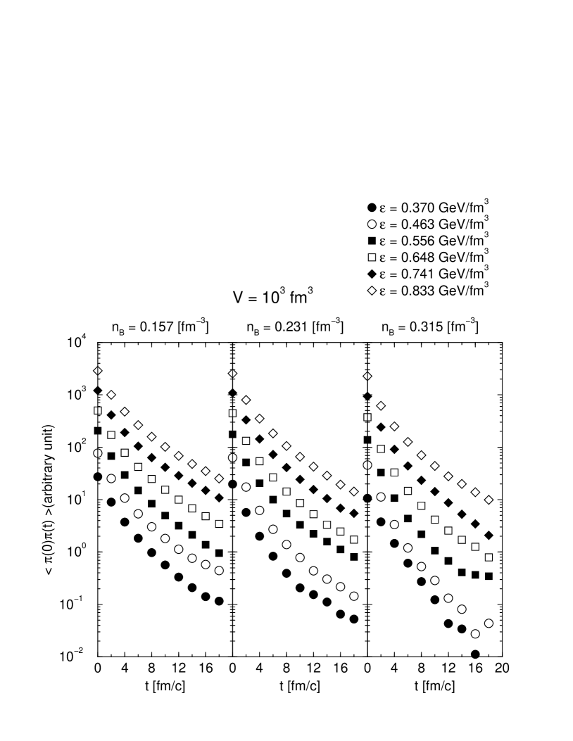
Figure 1: Relaxation in visous-shear tensor correlation

In a previous paper we have reported the calculation of transport coefficients of hadron gas based on a hadro-molecular simulation${}^{\cite[cite]{[\@@bibref{}{MS}{}{}]}}$. We used event generator URASiMA as a time evolution generator. In our simulation, we first put only baryons in the box with periodic boundary condition and turn switch on the simulator. Collisions between particles take place and mesons and resonances are produced. At later time, the system approaches to some kind of stationary state where all kinds of particle possess a common slope parameter, which we may call ”temperature”${}^{\cite[cite]{[\@@bibref{}{Sasaki-ptp}{}{}]}}$. The configurations of the stationary state we use as statistical ensembles.

Figure 1 displays correlation of stress-shear tensors as a function of time interval of the currents, which correspond to $(T_{xy}({\mbox{\boldmath${x}$}},t),T_{xy}({\mbox{\boldmath${x}$}}^{\prime},t^{\prime}))$ in the formula of the linear response theory. Figures 2 and 3 display the shear viscosity and heat conductivity of hadron gas obtained by our simulation. According to our simulation, both transport coefficients depend on baryon number density very weakly and temperature dependences are as strong as almost $T^{5}$${}^{\cite[cite]{[\@@bibref{}{MS}{}{}]}}$.

On the other hand, the changes of the relaxation times of the currents are very mild as functions of temperature (figs. 4 and 5). Most part of the temperature dependences of the transport coefficients come from the change of the intensity (expectation value of the current square (figs. 6 and 7)).

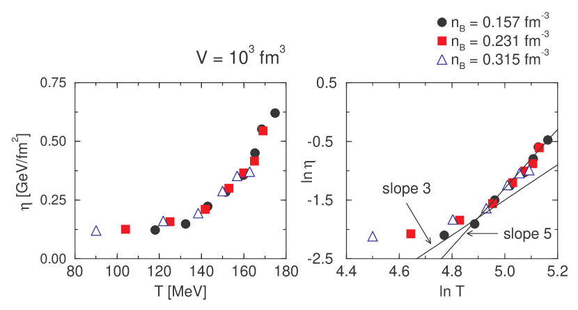
Figure 2: Shear visosity

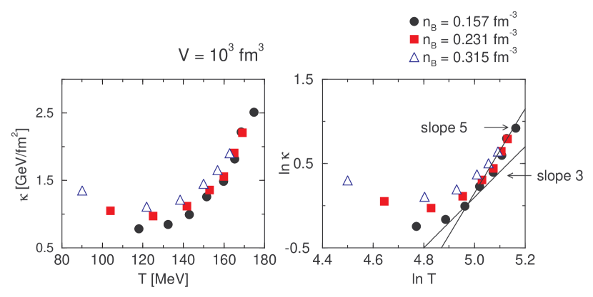
Figure 3: Heat concuctivity

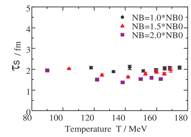
Figure 4: relaxation of visous-shear tensor

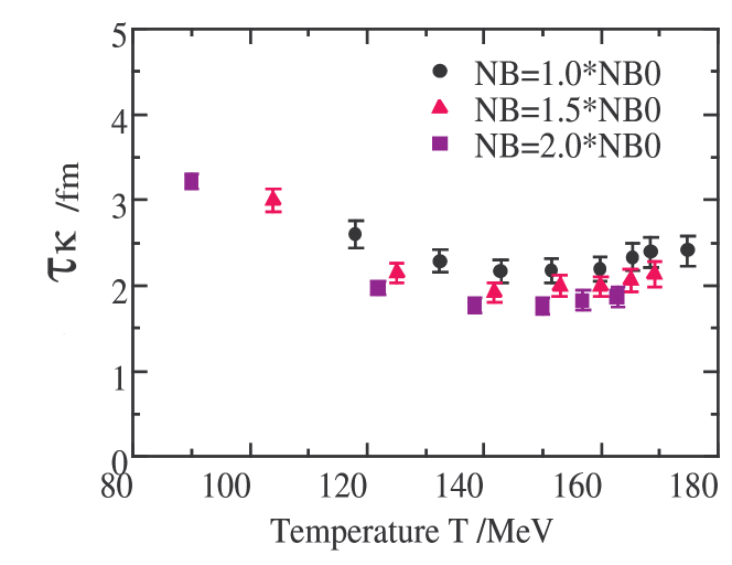
Figure 5: relaxation of heat conductivety

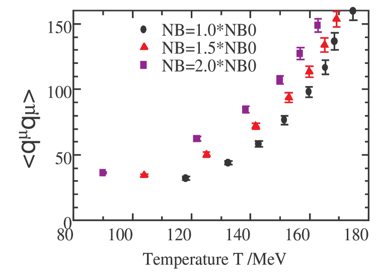
Figure 6: The square expectation of heat current

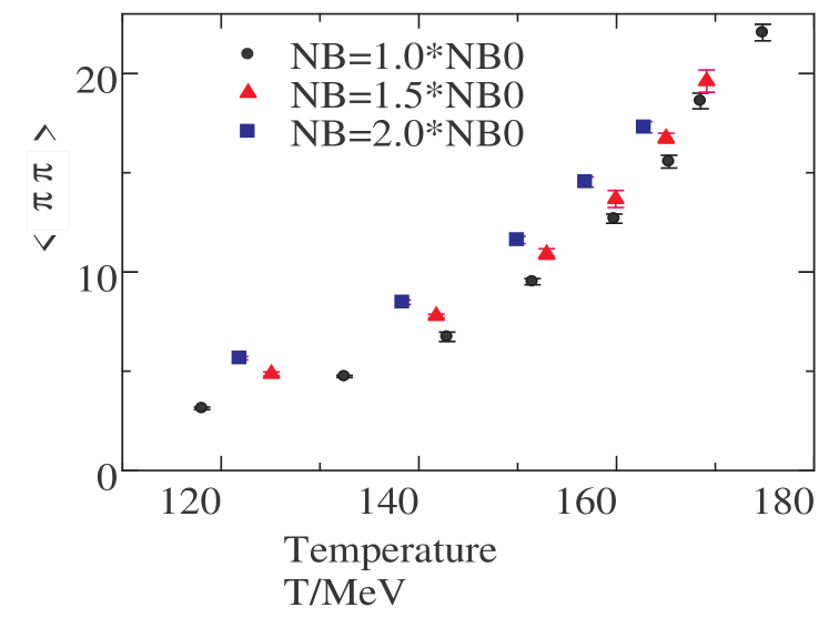
Figure 7: The square expectation of visous-shear tensor

6 Concluding remarks

In this paper we have investigated the coefficients of the causal hydrodyanamics and evaluated them by using a hadro-molecular simulation. According to our simulation based on URASiMA, the relaxation time of stress-shear tensor and heat current of the hadron gas are about 2 fm. The changes with temperature and baryon number density are very small. This results show rather clear contrast against the relaxation time in diffusion process which changes clearly with temperature ${}^{\cite[cite]{[\@@bibref{}{PRC,EPL}{}{}]}}$.

The importance of quantitatively investigating the relaxation in order to justify the macroscopic model has been pointed out by Iso, Mori and Namiki${}^{\cite[cite]{[\@@bibref{}{IMN}{}{}]}}$.

This work is supported by Grant-in-Aid for Scientific Research by Monbu-kagakusyo (No. 18540294). Stimulating discussions at the workshop ThermalField Theory and Its Application held at the Yukawa Institute for Theoretical Physics was extremely helpful.

References

- [1] L. D. Landau and E. M. Lifsitz, Fluid Mechanics(Pergamon Press, Oxford)1989.
- [2] M. Namiki and C. Iso, Prog. Theor. Phys. 18 (1957), 591.
- [3] S. Weinberg, Astrophys. J. 168 (1971), 175.
- [4] W. Israel, Ann. of Phys. 100, 310(76);W. Israel and J. M. Stewart, Ann. of Phys. 118, 341(79).
- [5] A. Muronga, Phys. Rev. C69 (2004), 034903;U. W. Heinz, H. Song and A. K. Chaudhuri, Phys. Rev. C73 (2006), 034904;A. Muronga, D. H. Rischke, nucl-th/0407114;R. Baier, P. Romatschke and U. A. Wiedemann, Phys. Rev. C73 (2006),064903.
- [6] S. Muroya and N. Sasaki, Prog. Theor. Phys. 113(2005), 457.
- [7] N. Sasaki, Prog. Theor. Phys. 106 (2001), 783.
- [8] N. Sasaki, O. Miyamura, S. Muroya and C. Nonaka, Phys. Rev. C 62 (2000), 011901R.
- [9] N. Sasaki, O. Miyamura, S. Muroya and C. Nonaka, Europhys. Lett. 54 (2001), 38.
- [10] C. Iso, K. Mori and M. Namiki, Prog. Theor. Phys. 22 (1959), 403.