The Three Site Model at One-Loop

Abstract:

In this paper we compute the one-loop chiral logarithmic corrections to all ${\cal O}(p^{4})$ counterterms in the three site Higgsless model. The calculation is performed using the background field method for both the chiral- and gauge-fields, and using Landau gauge for the quantum fluctuations of the gauge fields. The results agree with our previous calculations of the chiral-logarithmic corrections to the $S$ and $T$ parameters in ’t Hooft-Feynman gauge. The work reported here includes a complete evaluation of all one-loop divergences in an $SU(2)\times U(1)$ nonlinear sigma model, corresponding to an electroweak effective Lagrangian in the absence of custodial symmetry.

March 7, 2007

1 Introduction

Higgsless models [1] achieve electroweak symmetry breaking without introducing a fundamental scalar Higgs boson [2], and the unitarity of longitudinally-polarized $W$ and $Z$ boson scattering is preserved by the exchange of extra vector bosons [3, 4, 5, 6]. Inspired by TeV-scale [7] compactified five-dimensional gauge theories [8, 9, 10, 11], these models provide effectively unitary descriptions of the electroweak sector beyond the TeV energy scale.

Five-dimensional gauge-theories are not renormalizable, and therefore Higgsless models can only be viewed as effective theories valid below some high-energy cutoff (above which some other physics, a “high-energy” completion, must be present). Since these theories are only low-energy effective theories their properties may be conveniently studied using deconstruction [12, 13], which is a technique to build a four-dimensional gauge theory, with an appropriate gauge-symmetry breaking pattern, which approximates the properties of a five-dimensional theory. Deconstructed Higgsless models [14, 15, 16, 17, 18, 19, 20] have been used as tools to compute the general properties of Higgsless theories, and to illustrate the phenomological properties of this class of models.

The simplest deconstructed Higgsless model [21] incorporates only three sites on the deconstructed lattice, and the only additional vector states (other than the usual electroweak gauge bosons) are a triplet of $\rho^{\pm}$ and $\rho^{0}$ mesons (which may be interpreted as the lightest Kaluza-Klein states of a compactified five-dimensional theory). This theory is in the same class as models of extended electroweak gauge symmetries [22, 23] motivated by models of hidden local symmetry [24, 25, 26, 27, 28] in QCD, and the gauge sector is precisely that of the BESS model [22]. While simple, the three site model is sufficiently rich [21] to describe the physics associated with fermion mass generation, as well as the fermion delocalization [29, 30, 31, 32, 33, 34, 35] required in order to accord with precision electroweak tests [36, 37, 38, 39, 40].

Recently, we have computed [41] the one-loop chiral logarithmic corrections to the $S$ and $T$ parameters [36, 37, 38] in the three site Higgsless model, in the limit $M_{W}\ll M_{\rho}\ll\Lambda$, where $\Lambda$ is the cutoff of the effective three site Higgsless theory. In ref. [41], the calculation was performed by directly computing the one-loop corrections to four-fermion scattering processes in ’t Hooft-Feynman gauge, including the ghost, unphysical Goldstone-boson, and appropriate “pinch” contributions [42, 43] required to obtain gauge-invariant results for the one-loop self-energy functions.

In this paper, we compute the one-loop corrections to all ${\cal O}(p^{4})$ counterterms in the three site Higgsless model, using the renormalization group equation (RGE) technique. The calculation here is performed using the background field method for both the chiral- and gauge-fields, and using Landau gauge for the quantum fluctuations of the gauge fields. Focusing on those corrections which contribute to $S$ and $T$, we find that our RGE results agree with the chiral-logarithmic corrections to the $S$ and $T$ parameters determined previously [41] in ’t Hooft-Feynman gauge, thereby establishing the gauge-invariance of our results directly. Our calculations include also a complete evaluation of all one-loop divergences in an $SU(2)\times U(1)$ nonlinear sigma model, corresponding to an electroweak effective Lagrangian in the absence of custodial symmetry.

The hierarchy of scales, $M_{W}\ll M_{\rho}\ll\Lambda$, implies that the calculation breaks up into two different energy regimes. For renormalization group scales $\mu$ such that $M_{\rho}<\mu<\Lambda$, we consider the running of the effective Lagrangian parameters in the full three site model (illustrated in Figure 1). Running in the three site model is discussed in Section 2. At an energy scale of order $M_{\rho}$, one must “integrate out” the $\rho$-meson, matching to an effective two site model (the electroweak chiral Lagrangian [45, 46, 47, 48, 49], illustrated in Figure 2). For renormalization group scales $\mu<M_{\rho}$, we consider the running of the parameters in the two site electroweak chiral Lagrangian. Both the matching of the three site to the two site model and the low-energy running in the two site model are discussed in Section 3. In Section 4, we discuss the chiral-logarithmic corrections to the $S$ and $T$ parameters, and discuss the correspondence of the RGE calculation with that presented in Ref. [41]. Section 5 contains a concluding summary of our results.

The appendices include a detailed description of the one-loop calculations leading to the RGE equations. The one-loop renormalization of the operators [45, 46, 47, 48, 49] in the $SU(2)\times SU(2)/SU(2)$ chiral Lagrangian was first undertaken in Refs. [50, 51, 52] and later discussed in the context of electroweak physics [53, 54]. We review the the RGE calculation in a gauged $SU(2)\times SU(2)$ model using the background field method for the chiral- and gauge-fields, and add a calculation of the renormalization of the operator associated with fermion delocalization effects. Then, in the same language, we report our RGE calculation for a gauged $SU(2)\times U(1)$ model. We then show that the results of these separate calculations may be combined to obtain the RGE equations for the three site gauged $SU(2)\times SU(2)\times U(1)$ model.

2 The Three Site Model

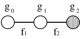
Figure 1: The moose diagram [55] for the three site model analyzed in this note. The $SU(2)$ gauge groups are shown as open circles, and the $U(1)$ gauge group is shown as a shaded circle. The fermion $SU(2)$ couplings arise from sites 0 and 1, and their hypercharge couplings from site 2 (c.f. eqn. (7)). The links, read from left to right, correspond to nonlinear sigma model fields $U_{1}$ and $U_{2}$ with $f$-constants $f_{1}$ and $f_{2}$, respectively.

In this section we consider the renormalization group structure of the three site model shown in Figure 1, valid for energies below the cutoff $\Lambda$ but above the mass of the heavy vector meson $M_{\rho}$.

2.1 The three site Lagrangian and counterterms

The lowest order (${\cal O}(p^{2})$) custodially symmetric Lagrangian of this model is given by

$${\cal L}_{2}=\sum_{i=1}^{2}\dfrac{f_{i}^{2}}{4}\mbox{tr}\left[(D_{\mu}U_{i})^{\dagger}(D^{\mu}U_{i})\right]-\sum_{i=0}^{2}\dfrac{1}{2g_{i}^{2}}\mbox{tr}\left[V_{i\mu\nu}V_{i}^{\mu\nu}\right],$$ (1)

where $D_{\mu}U_{i}$ and $V_{i\mu\nu}$ are defined as

$$D_{\mu}U_{i}\equiv\partial_{\mu}U_{i}+iV_{(i-1)\mu}U_{i}-iU_{i}V_{i\mu},$$ (2)

$$V_{i\mu\nu}\equiv\partial_{\mu}V_{i\nu}-\partial_{\nu}V_{i\mu}+i[V_{i\mu},V_{i\nu}].$$ (3)

The first two gauge fields ($i=0,1$) correspond to $SU(2)$ gauge groups,

$$V_{i\mu}=\sum_{a=1,2,3}\frac{\tau^{a}}{2}V^{a}_{i\mu},\qquad\mbox{for $i=0,1$},$$ (4)

while the last gauge field ($i=2$) corresponds to $U(1)$ group embedded as the $T_{3}$ generator of $SU(2)$,

$$V_{2\mu}=\frac{\tau^{3}}{2}V^{3}_{2\mu},\qquad\mbox{for $i=2$}.$$ (5)

There is one additional ${\cal O}(p^{2})$ term violating custodial symmetry,

$${\cal L}_{2}^{\prime}=\beta_{(2)}\dfrac{f_{2}^{2}}{4}\mbox{tr}\left[U_{2}^{\dagger}(D_{\mu}U_{2})\tau^{3}\right]\mbox{tr}\left[U_{2}^{\dagger}(D^{\mu}U_{2})\tau^{3}\right].$$ (6)

Fermions (quarks and leptons) couple to sites 0 and 1 (weak isospin), and to site 2 (weak hypercharge) through,

$${\cal L}_{f}=-2J_{W}^{a\mu}\,\mbox{tr}\left[\frac{\tau^{a}}{2}V_{0\mu}\right]-2x_{1}J_{W}^{a\mu}\,\mbox{tr}\left[\frac{\tau^{a}}{2}i(D_{\mu}U_{1})U_{1}^{\dagger}\right]-2J_{Y}^{\mu}\,\mbox{tr}\left[\frac{\tau^{3}}{2}V_{2\mu}\right],$$ (7)

where

$$J_{W}^{a\mu}\equiv\bar{\psi}_{L}\gamma^{\mu}T^{a}\psi_{L},\qquad J_{Y}^{\mu}\equiv\bar{\psi}_{L}\gamma^{\mu}Y_{\psi_{L}}\psi_{L}+\bar{\psi}_{R}\gamma^{\mu}Y_{\psi_{R}}\psi_{R},$$ (8)

and the $T^{a}$ and $Y_{\psi_{L},\psi_{R}}$ are the $SU(2)_{W}$ and $U(1)_{Y}$ charges of the fermions.

In order to renormalize the one-loop divergences of this model, we need to introduce appropriate counter terms at ${\cal O}(p^{4})$,

$${\cal L}_{4}=\sum_{i=1}^{2}{\cal L}_{4}^{(i)},$$ (9)

with

$${\cal L}_{4}^{(i)} = \alpha_{(i)1}\mbox{tr}\left[V_{(i-1)\mu\nu}U_{i}V_{i}^{\mu\nu}U_{i}^{\dagger}\right]$$ (10)

$$-2i\alpha_{(i)2}\mbox{tr}\left[(D_{\mu}U_{i})^{\dagger}(D_{\nu}U_{i})V_{i}^{\mu\nu}\right]$$

$$-2i\alpha_{(i)3}\mbox{tr}\left[V_{(i-1)}^{\mu\nu}(D_{\mu}U_{i})(D_{\nu}U_{i})^{\dagger}\right]$$

$$+\alpha_{(i)4}\mbox{tr}\left[(D_{\mu}U_{i})(D_{\nu}U_{i})^{\dagger}\right]\mbox{tr}\left[(D^{\mu}U_{i})(D^{\nu}U_{i})^{\dagger}\right]$$

$$+\alpha_{(i)5}\mbox{tr}\left[(D_{\mu}U_{i})(D^{\mu}U_{i})^{\dagger}\right]\mbox{tr}\left[(D_{\nu}U_{i})(D^{\nu}U_{i})^{\dagger}\right].$$

Here we have neglected terms violating the custodial symmetry at ${\cal O}(p^{4})$ level. Of the terms introduced in (6) and (10), the $\alpha_{(i)1}$ and $\beta_{(2)}$ will be of particular interest, as they contribute, respectively, to the precision electroweak parameters $\alpha S$ and $\alpha T$.

The three site model approximates (see [21] for details) the standard electroweak theory in the limit

$$g_{0}\ll g_{1}~{},\ \ \ \ \ \ \ g_{2}\ll g_{1}~{},$$ (11)

and we therefore define a small parameter $x=g_{0}/g_{1}\ll 1$. For simplicity, we also take $f_{1}=f_{2}$. The analysis of the three site model proceeds in an expansion in powers of $x$, and at tree-level the values of all electroweak observables differ from those in the standard model beginning at ${\cal O}(x^{2})$. To leading order, we find that $g_{0,2}$ are approximately equal to the standard model $SU(2)_{W}$ and $U(1)_{Y}$ couplings. Defining an angle $\theta$ such that $s\equiv\sin\theta$, $c\equiv\cos\theta$, and $s/c=g_{2}/g_{0}$, we find

$$g^{2}_{0}\approx\frac{4\pi\alpha}{s^{2}}=\frac{e^{2}}{s^{2}}~{},\ \ g^{2}_{2}\approx\frac{4\pi\alpha}{s^{2}}=\frac{e^{2}}{c^{2}}~{},$$ (12)

where $\alpha$ is the fine-structure constant and $e$ is the charge of the electron.

2.2 The Size of Electroweak and Radiative Corrections

To leading order, we find

$$\frac{M^{2}_{W}}{M^{2}_{\rho}}\approx\frac{x^{2}}{4}~{},$$ (13)

and [21, 41, 56] that the tree-level values

$$\alpha S^{tree} = \frac{4\pi\alpha}{g^{2}_{1}}\left(1-\frac{2x_{1}}{x^{2}}\right)$$ (14)

$$= \frac{4s^{2}M^{2}_{W}}{M^{2}_{\rho}}\left(1-\frac{x_{1}M^{2}_{\rho}}{2M^{2}_{W}}\right)~{},$$ (15)

$$\alpha T^{tree} = \beta_{(2)}~{},$$ (16)

summarize the deviations in the three site model relative to the standard electroweak theory.

Observationally, $\alpha S,\,\alpha T\leq{\cal O}(10^{-3})$ [39]. The mass of $M_{\rho}$ is bounded by ${\cal O}(1\,{\rm TeV})$, since $\rho$-exchange is necessary to maintain the unitarity of longitudinally polarized $W$-boson scattering – leading (from eqn. (15)) to a value of $\alpha S$ which is too large [17, 40] for localized fermions with $x_{1}=0$. The phenomenologically preferred region therefore has $x_{1}\approx x^{2}/2$,which is the condition for “ideal delocalization” [35, 56] in this model. In what follows, we will assume $x_{1}={\cal O}(x^{2})$.

As the observed limits on $\alpha S$ are ${\cal O}(10^{-3})$, radiative electroweak corrections are potentially important. In the context of the hierarchy $M_{W}\ll M_{\rho}\ll\Lambda$, the leading chiral logarithmic corrections are found to be of order [41]

$$\frac{\alpha}{4\pi}\log\frac{\Lambda}{M_{\rho}}~{},\ \ \ \frac{\alpha}{4\pi}\log\frac{M_{\rho}}{M_{H,{\rm ref}}}~{},\ \ {\rm or}\ \ \ \ \frac{\alpha\,x_{1}}{4\pi x^{2}}\log\frac{\Lambda}{M_{\rho}}~{},$$ (17)

where $M_{H,ref}$ is the reference Higgs mass used in the extraction of the value of $\alpha S$ from electroweak observations. As we shall see, the RGE calculations described here will allow us to reproduce the chiral log corrections found in Ref. [41], while simultaneously calculating the corrections to the other ${\cal O}(p^{4})$ chiral parameters. Given that $\alpha T$ is bounded by ${\cal O}(10^{-3})$, we will assume that the theory is approximately custodially symmetric and $\beta_{(2)}={\cal O}(\alpha/4\pi)$. In our computations, therefore, we will neglect contributions of order $\alpha\beta_{(2)}/4\pi$.

Inspired by AdS/CFT duality [57, 58, 59, 60], tree-level computations in this theory are interpreted to represent the leading terms in a large-$N$ expansion [61] of the strongly-coupled dual gauge theory akin to “walking technicolor” [62, 63, 64, 65, 66, 67]. Formally, both the electroweak [10, 41] and the chiral corrections [68, 69] are suppressed by $1/N$, and therefore the calculations presented here are consistent with duality. In this language, our discussion of the $S$ and $T$ parameters in the three site model will include (a) the tree-level contributions, which are of order $N$, (b) the chiral corrections which are order $1$ but enhanced by chiral logs, and (c) the effects of the $p^{4}$ counterterms, which are simply order $1$.

2.3 RGE Solutions in the three site model

Performing $\overline{\rm MS}$ renormalization of the one-loop amplitudes, we find that the chiral parameters (including, in particular, $\alpha_{(i)1}-\alpha_{(i)5}$ and $\beta_{(2)}$) depend on the renormalization scale $\mu$. The invariance of the amplitudes for physical processes with respect to changes in the renormalization scale $\mu$ gives rise to renormalization group equations (RGEs) for these chiral parameters in the usual manner. A detailed description of the calculation of the renormalization group equations, which is performed using the background field method for both the chiral- and gauge-fields and using Landau gauge for the quantum fluctuations of the gauge field, is given in appendix A of this paper. Here, we simply list the one-loop RGEs which result, for ${\cal O}(p^{2})$ parameters,

$$\mu\dfrac{d}{d\mu}f_{1}^{2} = \dfrac{3}{(4\pi)^{2}}(g_{0}^{2}+g_{1}^{2})f_{1}^{2},$$ (18)

$$\mu\dfrac{d}{d\mu}f_{2}^{2} = \dfrac{3}{(4\pi)^{2}}(g_{1}^{2}+\frac{1}{2}g_{2}^{2})f_{2}^{2},$$ (19)

$$\mu\dfrac{d}{d\mu}\left(\beta_{(2)}f_{2}^{2}\right) = \dfrac{3}{4(4\pi)^{2}}g_{2}^{2}f_{2}^{2},$$ (20)

for gauge coupling strengths,

$$\mu\dfrac{d}{d\mu}\left(\dfrac{1}{g_{0}^{2}}\right) = \dfrac{1}{(4\pi)^{2}}\left[\dfrac{44}{3}-\dfrac{1}{6}\right],$$ (21)

$$\mu\dfrac{d}{d\mu}\left(\dfrac{1}{g_{1}^{2}}\right) = \dfrac{1}{(4\pi)^{2}}\left[\dfrac{44}{3}-\dfrac{2}{6}\right],$$ (22)

$$\mu\dfrac{d}{d\mu}\left(\dfrac{1}{g_{2}^{2}}\right) = \dfrac{1}{(4\pi)^{2}}\left[\phantom{\dfrac{44}{3}}-\dfrac{1}{6}\right],$$ (23)

for ${\cal O}(p^{4})$ terms,

$$\mu\dfrac{d}{d\mu}\alpha_{(i)1} = \dfrac{1}{6(4\pi)^{2}},$$ (24)

$$\mu\dfrac{d}{d\mu}\alpha_{(i)2} = \dfrac{1}{12(4\pi)^{2}},$$ (25)

$$\mu\dfrac{d}{d\mu}\alpha_{(i)3} = \dfrac{1}{12(4\pi)^{2}},$$ (26)

$$\mu\dfrac{d}{d\mu}\alpha_{(i)4} = -\dfrac{1}{6(4\pi)^{2}},$$ (27)

$$\mu\dfrac{d}{d\mu}\alpha_{(i)5} = -\dfrac{1}{12(4\pi)^{2}},$$ (28)

and

$$\mu\dfrac{d}{d\mu}x_{1}=\dfrac{3g_{1}^{2}}{(4\pi)^{2}}x_{1},$$ (29)

for the fermion delocalization operator. Here we have assumed $\beta_{(2)}\ll 1$ and have ignored additional ${\cal O}(\beta_{(2)})$ terms in these RGEs.

Next we solve the renormalization group equations assuming

$$\beta_{(2)}\ll 1.$$ (30)

We find

$$f_{1}^{2}(\mu) = f_{1}^{2}(\Lambda)\exp\left[\int_{\Lambda}^{\mu}\dfrac{d\mu}{\mu}\dfrac{3}{(4\pi)^{2}}(g_{0}^{2}+g_{1}^{2})\right],$$ (31)

$$f_{2}^{2}(\mu) = f_{2}^{2}(\Lambda)\exp\left[\int_{\Lambda}^{\mu}\dfrac{d\mu}{\mu}\dfrac{3}{(4\pi)^{2}}(g_{1}^{2}+\frac{1}{2}g_{2}^{2})\right],$$ (32)

$$\beta_{(2)}(\mu) = \dfrac{3}{4(4\pi)^{2}}\int_{\Lambda}^{\mu}\dfrac{d\mu}{\mu}g_{2}^{2}(\mu),$$ (33)

for the ${\cal O}(p^{2})$ terms,

$$\dfrac{1}{g_{0}^{2}(\mu)} = \dfrac{1}{g_{0}^{2}(\Lambda)}+\dfrac{87}{6(4\pi)^{2}}\ln\dfrac{\mu}{\Lambda},$$ (34)

$$\dfrac{1}{g_{1}^{2}(\mu)} = \dfrac{1}{g_{1}^{2}(\Lambda)}+\dfrac{43}{3(4\pi)^{2}}\ln\dfrac{\mu}{\Lambda},$$ (35)

$$\dfrac{1}{g_{2}^{2}(\mu)} = \dfrac{1}{g_{2}^{2}(\Lambda)}-\dfrac{1}{6(4\pi)^{2}}\ln\dfrac{\mu}{\Lambda},$$ (36)

for the gauge-coupling strengths, and

$$x_{1}(\mu)=x_{1}(\Lambda)\exp\left[\int^{\mu}_{\Lambda}\dfrac{d\mu}{\mu}\dfrac{3g_{1}^{2}}{(4\pi)^{2}}\right],$$ (37)

for the delocalization parameter. We may similarly solve for the ${\cal O}(p^{4})$ coefficients. Here we list the results only for $\alpha_{(i)1}$’s explicitly

$$\alpha_{(1)1}(\mu) = \dfrac{1}{6(4\pi)^{2}}\ln\frac{\mu}{\Lambda}+\alpha_{(1)1}(\Lambda),$$ (38)

$$\alpha_{(2)1}(\mu) = \dfrac{1}{6(4\pi)^{2}}\ln\frac{\mu}{\Lambda}+\alpha_{(2)1}(\Lambda).$$ (39)

If we further assume

$$g_{0}^{2},g_{2}^{2}\ll g_{1}^{2},(4\pi)^{2},$$ (40)

we find

$$f_{1}^{2}(\mu) = f_{1}^{2}(\Lambda)\exp\left[\int_{\Lambda}^{\mu}\dfrac{d\mu}{\mu}\dfrac{3}{(4\pi)^{2}}g_{1}^{2}\right],$$ (41)

$$f_{2}^{2}(\mu) = f_{2}^{2}(\Lambda)\exp\left[\int_{\Lambda}^{\mu}\dfrac{d\mu}{\mu}\dfrac{3}{(4\pi)^{2}}g_{1}^{2}\right],$$ (42)

which, assuming $f^{2}_{1}(\Lambda)=f^{2}_{2}(\Lambda)$, justifies the ansatz

$$f_{1}^{2}(\mu)=f_{2}^{2}(\mu),$$ (43)

adopted in the discussion of the three site model in Refs.[21] and [41]. The assumption Eq.(40) also makes it possible to neglect the $\mu$ dependence of $g_{2}(\mu)$ in Eq.(33). We then find

$$\beta_{(2)}(\mu)=\dfrac{3}{4(4\pi)^{2}}g_{2}^{2}\ln\frac{\mu}{\Lambda}.$$ (44)

As demonstrated in the appendix, the three site RGE equations for $\alpha_{(i)1-5}$ arise solely from Goldstone Boson loops, and are therefore identical with those calculated [70, 28] in hidden local symmetry [24, 25, 26, 27, 28] models of QCD in the “vector limit” [71].

3 Matching to the Two Site Model and Running to Low Energies

In order to run to scales lower than $M_{\rho}$, we must integrate out the $\rho$-meson and match the three site model to the two site electroweak chiral lagrangian which describes the physics at scales below $M_{\rho}$. This matching is most conveniently done in two steps: first we reformulate the effect of fermion delocalization in terms of a redefinition of the chiral parameters in the three site lagrangian, a procedure described in the following subsection, and then we explicitly match the three site model to the two site model, as described in the second subsection. We conclude this section with a description of the running in the two site model for the energy range between $\mu=M_{\rho}$ and low energies $\mu=M_{H,ref}$.

3.1 Field redefinitions and fermion delocalization

We begin by reformulating the effect of fermion delocalization in terms of a redefinition of the chiral parameters in the three site lagrangian with brane-localized fermion couplings (to leading order in $x_{1}$). The delocalized fermion coupling in Eq.(7) can be written in a localized manner

$${\cal L}_{f}=-2J_{W}^{a\mu}\mbox{tr}\left[T^{a}W_{\mu}\right]-2J_{Y}^{\mu}\mbox{tr}\left[T^{3}B_{\mu}\right],$$ (45)

if we redefine the gauge fields as

$$W_{\mu} \equiv V_{0\mu}+x_{1}i(D_{\mu}U_{1})U_{1}^{\dagger},$$ (46)

$$B_{\mu} \equiv V_{2\mu}.$$ (47)

Note that $W_{\mu}$ transforms under the gauge symmetry in a manner similar to $V_{0\mu}$. Defining

$$\tilde{D}_{\mu}U_{1}\equiv\partial_{\mu}U_{1}+iW_{\mu}U_{1}-iU_{1}V_{1\mu},$$ (48)

we find

$$D_{\mu}U_{1}=\dfrac{1}{1-x_{1}}\tilde{D}_{\mu}U_{1},$$ (49)

and obtain

$$V_{0\mu}=W_{\mu}-\dfrac{x_{1}}{1-x_{1}}i(\tilde{D}_{\mu}U_{1})U_{1}^{\dagger}.$$ (50)

Defining the $W$ field strength $W_{\mu\nu}$ as

$$W_{\mu\nu}\equiv\partial_{\mu}W_{\nu}-\partial_{\nu}W_{\mu}+i[W_{\mu},W_{\nu}]~{},$$ (51)

we find that $V_{0\mu\nu}$ can be expressed in terms of $W_{\mu}$,

$$V_{0\mu\nu}=\dfrac{1}{1-x_{1}}W_{\mu\nu}-\dfrac{x_{1}}{1-x_{1}}U_{1}V_{1\mu\nu}U_{1}^{\dagger}-\dfrac{x_{1}}{(1-x_{1})^{2}}i[(\tilde{D}_{\mu}U_{1})U_{1}^{\dagger},(\tilde{D}_{\nu}U_{1})U_{1}^{\dagger}].$$ (52)

The ${\cal O}(p^{2})$ Lagrangian Eq.(1) may then be written as

$${\cal L}_{2} = \dfrac{f_{1}^{2}}{4}(1+2x_{1})\mbox{tr}\left[(\tilde{D}_{\mu}U_{1})^{\dagger}(\tilde{D}^{\mu}U_{1})\right]+\dfrac{f_{2}^{2}}{4}\mbox{tr}\left[(D_{\mu}U_{2})^{\dagger}(D^{\mu}U_{2})\right]$$ (53)

$$-\dfrac{1}{2g_{0}^{2}}(1+2x_{1})\mbox{tr}\left[W_{\mu\nu}W^{\mu\nu}\right]-\dfrac{1}{2g_{1}^{2}}\mbox{tr}\left[V_{1\mu\nu}V_{1}^{\mu\nu}\right]-\dfrac{1}{2g_{2}^{2}}\mbox{tr}\left[B_{\mu\nu}B^{\mu\nu}\right]$$

$$+\dfrac{x_{1}}{g_{0}^{2}}\mbox{tr}\left[W_{\mu\nu}U_{1}V_{1}^{\mu\nu}U_{1}^{\dagger}\right]-2\dfrac{x_{1}}{g_{0}^{2}}i\mbox{tr}\left[W_{\mu\nu}(\tilde{D}^{\mu}U_{1})(\tilde{D}^{\nu}U_{1})^{\dagger}\right]+{\cal O}(x_{1}^{2})~{}.$$

The ${\cal O}(p^{4})$ Lagrangians ${\cal L}_{4}^{(i)}$ become

$${\cal L}_{4}^{(1)} = \alpha_{(1)1}\mbox{tr}\left[W_{\mu\nu}U_{1}V_{1}^{\mu\nu}U_{1}^{\dagger}\right]$$ (54)

$$-2i\alpha_{(1)2}\mbox{tr}\left[(\tilde{D}_{\mu}U_{1})^{\dagger}(\tilde{D}_{\nu}U_{1})V_{1}^{\mu\nu}\right]$$

$$-2i\alpha_{(1)3}\mbox{tr}\left[W^{\mu\nu}(\tilde{D}_{\mu}U_{1})(\tilde{D}_{\nu}U_{1})^{\dagger}\right]$$

$$+\alpha_{(1)4}\mbox{tr}\left[(\tilde{D}_{\mu}U_{1})(\tilde{D}_{\nu}U_{1})^{\dagger}\right]\mbox{tr}\left[(\tilde{D}^{\mu}U_{1})(\tilde{D}^{\nu}U_{1})^{\dagger}\right]$$

$$+\alpha_{(1)5}\mbox{tr}\left[(\tilde{D}_{\mu}U_{1})(\tilde{D}^{\mu}U_{1})^{\dagger}\right]\mbox{tr}\left[(\tilde{D}_{\nu}U_{1})(\tilde{D}^{\nu}U_{1})^{\dagger}\right]+{\cal O}(x_{1}\alpha_{(i)j}),$$

and

$${\cal L}_{4}^{(2)} = \alpha_{(2)1}\mbox{tr}\left[V_{1\mu\nu}U_{2}B^{\mu\nu}U_{2}^{\dagger}\right]$$ (55)

$$-2i\alpha_{(2)2}\mbox{tr}\left[(D_{\mu}U_{2})^{\dagger}(D_{\nu}U_{2})B^{\mu\nu}\right]$$

$$-2i\alpha_{(2)3}\mbox{tr}\left[V_{1}^{\mu\nu}(D_{\mu}U_{2})(D_{\nu}U_{2})^{\dagger}\right]$$

$$+\alpha_{(2)4}\mbox{tr}\left[(D_{\mu}U_{2})(D_{\nu}U_{2})^{\dagger}\right]\mbox{tr}\left[(D^{\mu}U_{2})(D^{\nu}U_{2})^{\dagger}\right]$$

$$+\alpha_{(2)5}\mbox{tr}\left[(D_{\mu}U_{2})(D^{\mu}U_{2})^{\dagger}\right]\mbox{tr}\left[(D_{\nu}U_{2})(D^{\nu}U_{2})^{\dagger}\right]+{\cal O}(x_{1}\alpha_{(i)j}).$$

We note that the Lagrangian Eq.(53) now contains ${\cal O}(p^{4})$ terms. We thus rearrange Eq.(53) and Eq.(54) as

$$\tilde{{\cal L}}_{2} = \dfrac{\tilde{f}_{1}^{2}}{4}\mbox{tr}\left[(\tilde{D}_{\mu}U_{1})^{\dagger}(\tilde{D}^{\mu}U_{1})\right]+\dfrac{f_{2}^{2}}{4}\mbox{tr}\left[(D_{\mu}U_{2})^{\dagger}(D^{\mu}U_{2})\right]$$ (56)

$$-\dfrac{1}{2\tilde{g}_{0}^{2}}\mbox{tr}\left[W_{\mu\nu}W^{\mu\nu}\right]-\dfrac{1}{2g_{1}^{2}}\mbox{tr}\left[V_{1\mu\nu}V_{1}^{\mu\nu}\right]-\dfrac{1}{2g_{2}^{2}}\mbox{tr}\left[B_{\mu\nu}B^{\mu\nu}\right],$$

and

$$\tilde{{\cal L}}_{4}^{(1)} = \tilde{\alpha}_{(1)1}\mbox{tr}\left[W_{\mu\nu}U_{1}V_{1}^{\mu\nu}U_{1}^{\dagger}\right]$$ (57)

$$-2i\alpha_{(1)2}\mbox{tr}\left[(\tilde{D}_{\mu}U_{1})^{\dagger}(\tilde{D}_{\nu}U_{1})V_{1}^{\mu\nu}\right]$$

$$-2i\tilde{\alpha}_{(1)3}\mbox{tr}\left[W^{\mu\nu}(\tilde{D}_{\mu}U_{1})(\tilde{D}_{\nu}U_{1})^{\dagger}\right]$$

$$+\alpha_{(1)4}\mbox{tr}\left[(\tilde{D}_{\mu}U_{1})(\tilde{D}_{\nu}U_{1})^{\dagger}\right]\mbox{tr}\left[(\tilde{D}^{\mu}U_{1})(\tilde{D}^{\nu}U_{1})^{\dagger}\right]$$

$$+\alpha_{(1)5}\mbox{tr}\left[(\tilde{D}_{\mu}U_{1})(\tilde{D}^{\mu}U_{1})^{\dagger}\right]\mbox{tr}\left[(\tilde{D}_{\nu}U_{1})(\tilde{D}^{\nu}U_{1})^{\dagger}\right]+{\cal O}(x_{1}\alpha_{(i)j}),$$

with

$$\tilde{f}_{1}^{2} = f_{1}^{2}(1+2x_{1}),$$ (58)

$$\dfrac{1}{\tilde{g}_{0}^{2}} = \dfrac{1+2x_{1}}{g_{0}^{2}},$$ (59)

$$\tilde{\alpha}_{(1)1} = \alpha_{(1)1}+\dfrac{x_{1}}{g_{0}^{2}},$$ (60)

$$\tilde{\alpha}_{(1)3} = \alpha_{(1)3}+\dfrac{x_{1}}{g_{0}^{2}}.$$ (61)

3.2 Matching with the two site model

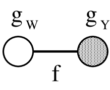
Figure 2: Moose diagram [55] for the two site electroweak chiral Lagrangian [45, 46, 47, 48, 49], an $SU(2)\times U(1)$ gauged nonlinear sigma model. The $SU(2)_{W}$ gauge group is shown as an open circle; the $U(1)_{Y}$ gauge group as a shaded circle. The link represents the nonlinear sigma model field $U$, with $f$-constant $f$.

Below the KK mass scale, phenomenology of the three site model can be described by a two site model, i.e., the electroweak chiral Lagrangian illustrated in Figure 2, with the ${\cal O}(p^{2})$ Lagrangian

$${\cal L}_{2}=\dfrac{f^{2}}{4}\mbox{tr}\left[(D_{\mu}U)^{\dagger}(D^{\mu}U)\right]-\dfrac{1}{2g_{W}^{2}}\mbox{tr}\left[W_{\mu\nu}W^{\mu\nu}\right]-\dfrac{1}{2g_{Y}^{2}}\mbox{tr}\left[B_{\mu\nu}B^{\mu\nu}\right]~{},$$ (62)

where

$$D_{\mu}U=\partial_{\mu}U+iW_{\mu}U-iUB_{\mu},\qquad U\equiv U_{1}U_{2}.$$ (63)

There also exists a custodial symmetry violating ${\cal O}(p^{2})$ operator

$${\cal L}_{2}^{\prime}=\beta\dfrac{f^{2}}{4}\mbox{tr}\left[U^{\dagger}(D_{\mu}U)\tau^{3}\right]\mbox{tr}\left[U^{\dagger}(D^{\mu}U)\tau^{3}\right]~{},$$ (64)

and the ${\cal O}(p^{4})$ operators

$${\cal L}_{4} = \alpha_{1}\mbox{tr}\left[W_{\mu\nu}UB^{\mu\nu}U^{\dagger}\right]$$ (65)

$$-2i\alpha_{2}\mbox{tr}\left[(D_{\mu}U)^{\dagger}(D_{\nu}U)B_{\mu\nu}\right]$$

$$-2i\alpha_{3}\mbox{tr}\left[W^{\mu\nu}(D_{\mu}U)(D_{\nu}U)^{\dagger}\right]$$

$$+\alpha_{4}\mbox{tr}\left[(D_{\mu}U)(D_{\nu}U)^{\dagger}\right]\mbox{tr}\left[(D^{\mu}U)(D^{\nu}U)^{\dagger}\right]$$

$$+\alpha_{5}\mbox{tr}\left[(D_{\mu}U)(D^{\mu}U)^{\dagger}\right]\mbox{tr}\left[(D_{\nu}U)(D^{\nu}U)^{\dagger}\right]~{}.$$

We next perform matching between three site and two site models. We will assume

$$\beta_{(2)},\alpha_{(i)1,2,3,4,5},x_{1}\ll 1,$$ (66)

and treat these parameters in a perturbative manner. In the limit $g_{0},g_{2}\ll g_{1}$, the mass-eigenstate $\rho$ field being integrated out is approximately the same as the field $V_{1\mu}$ of the three site model. Using the equations of motion arising from Eq. (56), to leading order in the derivative expansion

$$\frac{\delta\tilde{\cal L}_{2}}{\delta V_{1\mu}}=\partial_{\nu}\frac{\delta\tilde{\cal L}_{2}}{\delta(\partial_{\nu}V_{1\mu})}\approx 0~{},$$ (67)

this field may be expressed as

$$V_{1\mu}=\dfrac{1}{\tilde{f}_{1}^{2}+f_{2}^{2}}\left[\tilde{f}_{1}^{2}U_{1}^{\dagger}W_{\mu}U_{1}+f_{2}^{2}U_{2}B_{\mu}U_{2}^{\dagger}-i\tilde{f}_{1}^{2}U_{1}^{\dagger}\partial_{\mu}U_{1}-if_{2}^{2}U_{2}\partial_{\mu}U_{2}^{\dagger}\right].$$ (68)

From this we obtain

$$U_{1}^{\dagger}\tilde{D}_{\mu}U_{1} = \dfrac{f_{2}^{2}}{\tilde{f}_{1}^{2}+f_{2}^{2}}\left[U_{1}^{\dagger}\partial_{\mu}U_{1}-U_{2}\partial_{\mu}U_{2}^{\dagger}+iU_{1}^{\dagger}W_{\mu}U_{1}-iU_{2}B_{\mu}U_{2}^{\dagger}\right]$$ (69)

$$= \dfrac{f_{2}^{2}}{\tilde{f}_{1}^{2}+f_{2}^{2}}U_{1}^{\dagger}(D_{\mu}U)U_{2}^{\dagger},$$

$$U_{2}(D_{\mu}U_{2})^{\dagger} = \dfrac{\tilde{f}_{1}^{2}}{\tilde{f}_{1}^{2}+f_{2}^{2}}\left[-U_{1}^{\dagger}\partial_{\mu}U_{1}+U_{2}\partial_{\mu}U_{2}^{\dagger}-iU_{1}^{\dagger}W_{\mu}U_{1}+iU_{2}B_{\mu}U_{2}^{\dagger}\right]$$ (70)

$$= -\dfrac{\tilde{f}_{1}^{2}}{\tilde{f}_{1}^{2}+f_{2}^{2}}U_{1}^{\dagger}(D_{\mu}U)U_{2}^{\dagger},$$

$$V_{1\mu\nu} = \dfrac{\tilde{f}_{1}^{2}}{\tilde{f}_{1}^{2}+f_{2}^{2}}U_{1}^{\dagger}W_{\mu\nu}U_{1}+\dfrac{f_{2}^{2}}{\tilde{f}_{1}^{2}+f_{2}^{2}}U_{2}B_{\mu\nu}U_{2}^{\dagger}$$ (71)

$$+\dfrac{\tilde{f}_{1}^{2}f_{2}^{2}}{\left(\tilde{f}_{1}^{2}+f_{2}^{2}\right)^{2}}iU_{2}\left[U^{\dagger}(D_{\mu}U),U^{\dagger}(D_{\nu}U)\right]U_{2}^{\dagger}.$$

Putting these into Eqs. (6), (55), (56) and (57), we match the two site model to the three site model, and find matching conditions

$$\dfrac{1}{f^{2}} = \dfrac{1}{\tilde{f}_{1}^{2}}+\dfrac{1}{f_{2}^{2}}\simeq\dfrac{1}{f_{1}^{2}}+\dfrac{1}{f_{2}^{2}},$$ (72)

$$\beta = \beta_{(2)}\dfrac{\tilde{f}_{1}^{2}}{\tilde{f}_{1}^{2}+f_{2}^{2}}\simeq\beta_{(2)}\dfrac{f_{1}^{2}}{f_{1}^{2}+f_{2}^{2}},$$ (73)

$$\dfrac{1}{g_{W}^{2}} = \dfrac{1}{\tilde{g}_{0}^{2}}+\dfrac{1}{g_{1}^{2}}\left(\dfrac{\tilde{f}_{1}^{2}}{\tilde{f}_{1}^{2}+f_{2}^{2}}\right)^{2}-2\tilde{\alpha}_{(1)1}\left(\dfrac{\tilde{f}_{1}^{2}}{\tilde{f}_{1}^{2}+f_{2}^{2}}\right)$$ (74)

$$\simeq \dfrac{1}{g_{0}^{2}},$$

$$\dfrac{1}{g_{Y}^{2}} = \dfrac{1}{g_{2}^{2}}+\dfrac{1}{g_{1}^{2}}\left(\dfrac{f_{2}^{2}}{\tilde{f}_{1}^{2}+f_{2}^{2}}\right)^{2}-2\alpha_{(2)1}\left(\dfrac{f_{2}^{2}}{\tilde{f}_{1}^{2}+f_{2}^{2}}\right)$$ (75)

$$\simeq \dfrac{1}{g_{2}^{2}},$$

$$\alpha_{1} = -\dfrac{1}{g_{1}^{2}}\left(\dfrac{\tilde{f}_{1}f_{2}}{\tilde{f}_{1}^{2}+f_{2}^{2}}\right)^{2}+\tilde{\alpha}_{(1)1}\left(\dfrac{f_{2}^{2}}{\tilde{f}_{1}^{2}+f_{2}^{2}}\right)+\alpha_{(2)1}\left(\dfrac{\tilde{f}_{1}^{2}}{\tilde{f}_{1}^{2}+f_{2}^{2}}\right)$$ (76)

$$\simeq -\dfrac{1}{g_{1}^{2}}\dfrac{f_{1}^{2}f_{2}^{2}}{(f_{1}^{2}+f_{2}^{2})^{2}}+\left(\alpha_{(1)1}+\dfrac{x_{1}}{g_{0}^{2}}\right)\dfrac{f_{2}^{2}}{f_{1}^{2}+f_{2}^{2}}+\alpha_{(2)1}\dfrac{f_{1}^{2}}{f_{1}^{2}+f_{2}^{2}},$$

$$\alpha_{2} \simeq -\dfrac{1}{g_{1}^{2}}\dfrac{f_{1}^{2}f_{2}^{4}}{(f_{1}^{2}+f_{2}^{2})^{3}}+\alpha_{(2)1}\dfrac{f_{1}^{2}f_{2}^{2}}{(f_{1}^{2}+f_{2}^{2})^{2}}$$ (77)

$$+\alpha_{(1)2}\dfrac{f_{2}^{6}}{(f_{1}^{2}+f_{2}^{2})^{3}}+\alpha_{(2)2}\dfrac{f_{1}^{4}}{(f_{1}^{2}+f_{2}^{2})^{2}}+\alpha_{(2)3}\dfrac{f_{1}^{4}f_{2}^{2}}{(f_{1}^{2}+f_{2}^{2})^{3}},$$

$$\alpha_{3} \simeq -\dfrac{1}{g_{1}^{2}}\dfrac{f_{1}^{4}f_{2}^{2}}{(f_{1}^{2}+f_{2}^{2})^{3}}+\left(\alpha_{(1)1}+\dfrac{x_{1}}{g_{0}^{2}}\right)\dfrac{f_{1}^{2}f_{2}^{2}}{(f_{1}^{2}+f_{2}^{2})^{2}}$$ (78)

$$+\alpha_{(1)2}\dfrac{f_{1}^{2}f_{2}^{4}}{(f_{1}^{2}+f_{2}^{2})^{3}}+\left(\alpha_{(1)3}+\dfrac{x_{1}}{g_{0}^{2}}\right)\dfrac{f_{2}^{4}}{(f_{1}^{2}+f_{2}^{2})^{2}}+\alpha_{(2)3}\dfrac{f_{1}^{6}}{(f_{1}^{2}+f_{2}^{2})^{3}},$$

$$\alpha_{4} \simeq \frac{1}{g^{2}_{1}}\Bigg{(}\frac{f_{1}f_{2}}{f_{1}^{2}+f_{2}^{2}}\Bigg{)}^{4}-2\alpha_{(1)2}\frac{f_{1}^{2}f_{2}^{6}}{(f_{1}^{2}+f_{2}^{2})^{4}}-2\alpha_{(2)3}\frac{f_{1}^{6}f_{2}^{2}}{(f_{1}^{2}+f_{2}^{2})^{4}}$$ (79)

$$+\alpha_{(1)4}\Bigg{(}\frac{f_{2}^{2}}{f_{1}^{2}+f_{2}^{2}}\Bigg{)}^{4}+\alpha_{(2)4}\Bigg{(}\frac{f_{1}^{2}}{f_{1}^{2}+f_{2}^{2}}\Bigg{)}^{4}\,,$$

$$\alpha_{5} \simeq -\frac{1}{g^{2}_{1}}\Bigg{(}\frac{f_{1}f_{2}}{f_{1}^{2}+f_{2}^{2}}\Bigg{)}^{4}+2\alpha_{(1)2}\frac{f_{1}^{2}f_{2}^{6}}{(f_{1}^{2}+f_{2}^{2})^{4}}+2\alpha_{(2)3}\frac{f_{1}^{6}f_{2}^{2}}{(f_{1}^{2}+f_{2}^{2})^{4}}$$ (80)

$$+\alpha_{(1)5}\Bigg{(}\frac{f_{2}^{2}}{f_{1}^{2}+f_{2}^{2}}\Bigg{)}^{4}+\alpha_{(2)5}\Bigg{(}\frac{f_{1}^{2}}{f_{1}^{2}+f_{2}^{2}}\Bigg{)}^{4}~{},$$

where we match at a scale

$$\mu=M_{\rho}\simeq g_{1}\dfrac{\sqrt{f_{1}^{2}+f_{2}^{2}}}{2}.$$ (81)

Finally, we note that we can make contact with prior results by setting $f_{1}=f_{2}$ and $\alpha_{(i)j}=0$. In this limit, Eqs.(76)–(80) lead to

$$\alpha_{1}=-\dfrac{1}{4g_{1}^{2}} + \dfrac{x_{1}}{2g_{0}^{2}},\qquad\alpha_{2}=-\dfrac{1}{8g_{1}^{2}},\qquad\alpha_{3}=-\dfrac{1}{8g_{1}^{2}}+\dfrac{x_{1}}{2g_{0}^{2}},$$ (82)

$$\alpha_{4} = \frac{1}{16g_{1}^{2}},\qquad\qquad\alpha_{5}=-\frac{1}{16g_{1}^{2}},$$ (83)

which are consistent with Table 2 given in  [21].

3.3 Solutions of RGE in the two site model

We next consider the renormalization group flow in the two site model, from a scale $\mu=M_{\rho}$ to low-energy, $\mu=M_{H,{\rm ref}}$. The renormalization group equations of the two site model, the derivation of which is described in A.2, are given by

$$\mu\dfrac{d}{d\mu}f^{2} = \dfrac{3}{(4\pi)^{2}}(g_{W}^{2}+\frac{1}{2}g_{Y}^{2})f^{2},$$ (84)

$$\mu\dfrac{d}{d\mu}\left(\beta f^{2}\right) = \dfrac{3}{4(4\pi)^{2}}g_{Y}^{2}f^{2},$$ (85)

$$\mu\dfrac{d}{d\mu}\left(\dfrac{1}{g_{W}^{2}}\right) = \dfrac{1}{(4\pi)^{2}}\left[\dfrac{44}{3}-\dfrac{1}{6}\right],$$ (86)

$$\mu\dfrac{d}{d\mu}\left(\dfrac{1}{g_{Y}^{2}}\right) = \dfrac{1}{(4\pi)^{2}}\left[\phantom{\dfrac{44}{3}}-\dfrac{1}{6}\right],$$ (87)

$$\mu\dfrac{d}{d\mu}\alpha_{1} = \dfrac{1}{6(4\pi)^{2}},$$ (88)

$$\mu\dfrac{d}{d\mu}\alpha_{2} = \dfrac{1}{12(4\pi)^{2}},$$ (89)

$$\mu\dfrac{d}{d\mu}\alpha_{3} = \dfrac{1}{12(4\pi)^{2}},$$ (90)

$$\mu\dfrac{d}{d\mu}\alpha_{4} = -\dfrac{1}{6(4\pi)^{2}},$$ (91)

$$\mu\dfrac{d}{d\mu}\alpha_{5} = -\dfrac{1}{12(4\pi)^{2}}.$$ (92)

We solve these equations assuming

$$\beta\ll 1.$$ (93)

We find

$$\beta(\mu)=\frac{3}{4}\dfrac{g_{Y}^{2}}{(4\pi)^{2}}\ln\dfrac{\mu}{M_{\rho}}+\beta(M_{\rho}),$$ (94)

and

$$\alpha_{1}(\mu) = \dfrac{1}{6(4\pi)^{2}}\ln\frac{\mu}{M_{\rho}}+\alpha_{1}(M_{\rho}),$$ (95)

and similarly for the other $\alpha_{i}$.

4 $\alpha S$ and $\alpha T$

Using the results of Sections 2 and 3, we may compute the values of $\alpha S$ and $\alpha T$, which are defined as

$$\alpha S = -16\pi\alpha\,\alpha_{1}(\mu=M_{H,\rm ref}),$$ (96)

$$\alpha T = 2\beta(\mu=M_{H,\rm ref}).$$ (97)

We begin with Eqn. (96) and use the RGE equations to evaluate $\alpha S$ at successively higher energy scales, and eventually compare it with the results in Ref. [41]. First, we can use Eqn. (95) to run up from $M_{H,\rm ref}$ to $M_{\rho}$

$$\alpha S=-16\pi\alpha\,\alpha_{1}(M_{\rho})-\dfrac{\alpha}{6\pi}\ln\dfrac{M_{H,\rm ref}}{M_{\rho}}.$$ (98)

Taking $f_{1}=f_{2}$, we apply Eqn. (76) to match from the two-site to the three-site regime

$$\alpha S\simeq\dfrac{4\pi\alpha}{g_{1}^{2}(M_{\rho})}-8\pi\alpha\,\alpha_{(1)1}(M_{\rho})-8\pi\alpha\,\alpha_{(2)1}(M_{\rho})-\dfrac{8\pi\alpha x_{1}(M_{\rho})}{g_{0}^{2}(M_{\rho})}-\dfrac{\alpha}{6\pi}\ln\dfrac{M_{H,\rm ref}}{M_{\rho}}.$$ (99)

We employ Eqns. (37, 38, 39) to run $x_{1}$, $\alpha_{(1)1}$, and $\alpha_{(2)1}$ up to scale $\Lambda$

$$\alpha S \simeq \dfrac{4\pi\alpha}{g_{1}^{2}(M_{\rho})}-\dfrac{\alpha}{6\pi}\ln\dfrac{M_{H,\rm ref}}{M_{\rho}}-\dfrac{\alpha}{6\pi}\ln\dfrac{M_{\rho}}{\Lambda}-8\pi\alpha\,\alpha_{(1)1}(\Lambda)-8\pi\alpha\,\alpha_{(2)1}(\Lambda)$$ (100)

$$-\dfrac{8\pi\alpha x_{1}(\Lambda)}{g_{0}^{2}(\Lambda)}\exp\left[\int^{M_{\rho}}_{\Lambda}\dfrac{d\mu}{\mu}\dfrac{3g_{1}^{2}(\mu)}{(4\pi)^{2}}\right],$$

and then employ Eqn. (35) to run $g_{1}$ up to scale $\Lambda$

$$\alpha S \simeq \dfrac{4\pi\alpha}{g_{1}^{2}(\Lambda)}-\dfrac{8\pi\alpha x_{1}(\Lambda)}{g_{0}^{2}(\Lambda)}-\dfrac{\alpha}{6\pi}\ln\dfrac{M_{H,\rm ref}}{M_{\rho}}+\dfrac{41\alpha}{12\pi}\ln\dfrac{M_{\rho}}{\Lambda}-\dfrac{3\alpha}{2\pi}\dfrac{x_{1}g_{1}^{2}}{g_{0}^{2}}\ln\dfrac{M_{\rho}}{\Lambda}$$ (101)

$$-8\pi\alpha\,\alpha_{(1)1}(\Lambda)-8\pi\alpha\,\alpha_{(2)1}(\Lambda).$$

In the first line of Eq.(101), we have used the expansion

$$\exp\left[\int^{M_{\rho}}_{\Lambda}\dfrac{d\mu}{\mu}\dfrac{3g_{1}^{2}(\mu)}{(4\pi)^{2}}\right]\simeq 1+\dfrac{3}{(4\pi)^{2}}g_{1}^{2}\ln\dfrac{M_{\rho}}{\Lambda}.$$ (102)

In order to make connection with the results of ref. [41], we note that at tree-level

$$M^{2}_{W}\approx\frac{g^{2}_{0}f^{2}}{4}=\frac{g^{2}_{0}f^{2}_{1}}{8}~{},$$ (103)

and, therefore (c.f. Eq. (81)),

$$\frac{g^{2}_{1}}{g^{2}_{0}}=\frac{M^{2}_{\rho}}{4M^{2}_{W}}~{},$$ (104)

so that the first two terms of Eqn. (101) may be rewritten as

$$\dfrac{4\pi\alpha}{g_{1}^{2}(\Lambda)}-\dfrac{8\pi\alpha x_{1}(\Lambda)}{g_{0}^{2}(\Lambda)}=\left[\frac{4s^{2}M^{2}_{W}}{M^{2}_{\rho}}\left(1-\frac{x_{1}M^{2}_{\rho}}{2M^{2}_{W}}\right)\right]_{\mu=\Lambda}~{},$$ (105)

to this order.

Similarly, starting from Eqn. (97), we can use the RGE equations from the previous sections to evaluate $\alpha T$ at higher energy scales, and eventually compare it with the results in Ref. [41]. First, we can use Eqn. (94) to run up from $M_{H,\rm ref}$ to $M_{\rho}$

$$\alpha T=2\beta(M_{\rho})+\dfrac{3g_{Y}^{2}}{2(4\pi)^{2}}\ln\dfrac{M_{H,\rm ref}}{M_{\rho}}.$$ (106)

Taking $f_{1}=f_{2}$, we apply Eqn. (73) to match from the two-site to the three-site regime

$$\alpha T=\beta_{(2)}(M_{\rho})+\dfrac{3g_{Y}^{2}}{2(4\pi)^{2}}\ln\dfrac{M_{H,\rm ref}}{M_{\rho}},$$ (107)

and then employ Eqn. (44) to run up to scale $\Lambda$

$$\alpha T = \beta_{(2)}(\Lambda)+\dfrac{3g_{2}^{2}}{4(4\pi)^{2}}\ln\dfrac{M_{\rho}}{\Lambda}+\dfrac{3g_{Y}^{2}}{2(4\pi)^{2}}\ln\dfrac{M_{H,\rm ref}}{M_{\rho}}$$ (108)

$$\simeq \beta_{(2)}(\Lambda)+\dfrac{3g_{Y}^{2}}{4(4\pi)^{2}}\ln\dfrac{M_{\rho}}{\Lambda}+\dfrac{3g_{Y}^{2}}{2(4\pi)^{2}}\ln\dfrac{M_{H,\rm ref}}{M_{\rho}}.$$

We can now see that our leading-log expressions for $\alpha S$ (101) and $\alpha T$ (108) correspond exactly to those found in [41]. Note that the calculations in [41] are performed in ’t Hooft-Feynman gauge, whereas those reported here are performed in Landau gauge. The correspondence of these calculations is therefore an explicit demonstration of the gauge-invariance of the results. In addition, as noted in [41], the $M_{H,{\rm ref}}$ dependence of the results in Eqns. (101) and (108) matches that of the low-energy effective theory of the standard model with a heavy Higgs boson [45, 46, 47, 48], and therefore these contributions are model-independent and match the dependence on the reference Higgs-boson mass present in the experimental determinations of $\alpha S$ and $\alpha T$.

Our expressions for the $S$ and $T$ parameters include (a) the tree-level contributions, which are of order $N$, (b) the chiral corrections which are order $1$ but enhanced by chiral logs, and (c) the effects of the $p^{4}$ counterterms, which are simply order $1$. While the coefficients of the counterterms are unknown, it is important to note that their magnitude is sub-leading in the large-$N$ expansion. A detailed investigation of the size of the chiral log corrections, and of the corresponding phenomenological bounds on the three site model, is underway [72].

5 Summary

In this paper we have computed the one-loop chiral logarithmic corrections to all ${\cal O}(p^{4})$ counterterms in the three site Higgsless model. The calculation is performed using the background field method for both the chiral- and gauge-fields, and using Landau gauge for the quantum fluctuations of the gauge fields. For the chiral parameters $\alpha_{(i)1-5}$, the contributions to the RGE equations arise solely from Goldstone Boson loops, and are therefore identical with those calculated [70] in hidden local symmetry [24, 25, 26, 27, 28] models of QCD in the “vector limit” [71]. Our results agree with previous calculations [41] of the chiral-logarithmic corrections to the $S$ and $T$ parameters in ’t Hooft-Feynman gauge.

Acknowledgments

We thank Kaoru Hagiwara and Qi-Shu Yan for discussions on the renormalization of $SU(2)\times U(1)$ gauged nonlinear sigma model. The visit of S.M. to Michigan State University which made this collaboration possible was fully supported by the fund of The Mitsubishi Foundation through Koichi Yamawaki, and this work received the preliminary report number DPNU-06-12. R.S.C. and E.H.S. are supported in part by the US National Science Foundation under grant PHY-0354226. M.T.’s work is supported in part by the JSPS Grant-in-Aid for Scientific Research No.16540226

Appendix A RGE Calculations

In this appendix, we outline the calculation of the renormalization group equations used in this paper. All calculations are performed using dimensional regularization, renormalized using modified minimal subtraction ($\overline{\rm MS}$). In order to facilitate the identification of the counterterms required, the calculations are performed using the background field method for both the chiral- and gauge-fields. Landau gauge, in which all unphysical Goldstone bosons and ghost fields are massless, is used for the quantum fluctuations of the gauge fields.

The calculation is carried out in three steps. In the next subsection, A.1, we discuss the RGE calculation in the context of a gauged $SU(2)\times SU(2)$ model. In the following subsection, A.2, we discuss the RGE calculation in a gauged $SU(2)\times U(1)$ model. Finally, in the last subsection, A.3, we show how these results may be combined to obtain the RGE equations for the three site gauged $SU(2)\times SU(2)\times U(1)$ model. The results of the last subsection yield the equations necessary for section 2.3: running from high-energies, $\mu=\Lambda$, to intermediate energies, $\mu=M_{\rho}$. The results of the second subsection directly yield the equations necessary for section 3.3: running between intermediate energies and low energies, $\mu=M_{H,{\rm ref}}$.

The divergences of the scalar one-loop integrals which appear are discussed, in general form, in appendix B.

A.1 $SU(2)\times SU(2)$ gauged nonlinear sigma model

The one-loop renormalization of the operators [45, 46, 47, 48, 49] in the $SU(2)\times SU(2)/SU(2)$ chiral Lagrangian was first undertaken in Refs. [50, 51, 52] and later discussed in the context of electroweak physics [53, 54]. Here we review the the RGE calculation in a gauged $SU(2)\times SU(2)$ model using the background field method for the chiral- and gauge-fields, and add a calculation of the renormalization of the operator associated with fermion delocalization effects.

Figure 3: Moose diagram for the $SU(2)\times SU(2)$ gauged nonlinear sigma model analyzed in this subsection. $SU(2)$ gauge groups are shown as open circles.

We begin by considering an $SU(2)\times SU(2)$ gauged nonlinear sigma model shown in a moose diagram Figure 3. The lowest order (${\cal O}(p^{2})$) Lagrangian of this model is given by

$${\cal L}_{2}=\dfrac{f^{2}}{4}\mbox{tr}\left[(D_{\mu}U)^{\dagger}(D^{\mu}U)\right]-\dfrac{1}{2g_{0}^{2}}\mbox{tr}\left[V_{0\mu\nu}V_{0}^{\mu\nu}\right]-\dfrac{1}{2g_{1}^{2}}\mbox{tr}\left[V_{1\mu\nu}V_{1}^{\mu\nu}\right],$$ (A.109)

with $U$ being a chiral field,

$$U\equiv\exp\left[\dfrac{2i\pi^{a}T^{a}}{f}\right],\qquad T^{a}\equiv\dfrac{\tau^{a}}{2}.$$ (A.110)

The gauge field strengths $V_{0\mu\nu}$ and $V_{1\mu\nu}$ are defined as

$$V_{0\mu\nu}\equiv\partial_{\mu}V_{0\nu}-\partial_{\nu}V_{0\mu}+i[V_{0\mu},V_{0\nu}],\qquad V_{1\mu\nu}\equiv\partial_{\mu}V_{1\nu}-\partial_{\nu}V_{1\mu}+i[V_{1\mu},V_{1\nu}],$$ (A.111)

with $V_{0\mu}$ and $V_{1\mu}$ being the gauge fields at site-0 and site-1 in the moose diagram,

$$V_{0\mu}\equiv V^{a}_{0\mu}T^{a},\qquad V_{1\mu}\equiv V^{a}_{1\mu}T^{a}.$$ (A.112)

The covariant derivative $D_{\mu}U$ is given by

$$D_{\mu}U\equiv\partial_{\mu}U+iV_{0\mu}U-iUV_{1\mu}.$$ (A.113)

We calculate one-loop divergences using the background field formalism in order to maintain manifest chiral and gauge invariance. For this purpose we decompose the chiral field $U$ into a background field $\bar{U}$ and a fluctuating quantum Nambu-Goldstone Boson (NGB) field $u^{a}$,

$$U=\bar{U}\exp\left[\dfrac{2iu^{a}T^{a}}{f}\right].$$ (A.114)

In a similar manner, we decompose the site-1 gauge field $V_{1\mu}$ into a background field $\bar{V}_{1\mu}$ and a quantum field $v_{1\mu}$,

$$V_{1\mu}=\bar{V}_{1\mu}+g_{1}v_{1\mu}.$$ (A.115)

For the site-0 gauge field $V_{0\mu}$, it is convenient to first make a gauge transformation,

$$V_{0\mu}\to V^{\prime}_{0\mu}=\bar{U}^{\dagger}V_{0\mu}\bar{U}-i\bar{U}^{\dagger}\partial_{\mu}\bar{U},$$ (A.116)

and then decompose it into a background field $\bar{V}_{0\mu}$ and a quantum field $v_{0\mu}$,

$$V^{\prime}_{0\mu}=\bar{V}_{0\mu}+g_{0}v_{0\mu}.$$ (A.117)

Expanding the ${\cal O}(p^{2})$ Lagrangian Eq.(A.109) in terms of these quantum fields $u$ and $v_{\mu}$, we obtain

$${\cal L}_{2}=\left.{\cal L}_{2}\right|_{0}+\left.{\cal L}_{2}\right|_{u}+\left.{\cal L}_{2}\right|_{v}+\left.{\cal L}_{2}\right|_{uu}+\left.{\cal L}_{2}\right|_{vv}+\left.{\cal L}_{2}\right|_{uv}+\cdots,$$ (A.118)

with

$$\left.{\cal L}_{2}\right|_{0} = \dfrac{f^{2}}{4}\mbox{tr}\left[(\bar{V}_{0\mu}-\bar{V}_{1\mu})(\bar{V}_{0}^{\mu}-\bar{V}_{1}^{\mu})\right]-\dfrac{1}{2g_{0}^{2}}\mbox{tr}\left[\bar{V}_{0\mu\nu}\bar{V}_{0}^{\mu\nu}\right]-\dfrac{1}{2g_{1}^{2}}\mbox{tr}\left[\bar{V}_{1\mu\nu}\bar{V}_{1}^{\mu\nu}\right],$$ (A.119)

$$\left.{\cal L}_{2}\right|_{u} = \dfrac{f}{2}\partial_{\mu}u^{a}(\bar{V}_{0}^{a\mu}-\bar{V}_{1}^{a\mu})-\dfrac{f}{2}\epsilon^{abc}\bar{V}_{0\mu}^{a}\bar{V}_{1}^{b\mu}u^{c},$$ (A.120)

$$\left.{\cal L}_{2}\right|_{v} = \dfrac{f^{2}}{4}(\bar{V}_{0\mu}^{a}-\bar{V}_{1\mu}^{a})(g_{0}v_{0}^{\mu}-g_{1}v_{1}^{\mu})-\frac{1}{g_{0}}\bar{V}_{0\mu\nu}^{a}(D^{\mu}v_{0}^{\nu})^{a}-\frac{1}{g_{1}}\bar{V}_{1\mu\nu}^{a}(D^{\mu}v_{1}^{\nu})^{a},$$ (A.121)

$$\left.{\cal L}_{2}\right|_{uu} = \frac{1}{2}(D_{\mu}u)^{a}(D^{\mu}u)^{a}-\frac{1}{8}\epsilon^{abc}\epsilon^{ade}(\bar{V}_{0\mu}^{b}-\bar{V}_{1\mu}^{b})u^{c}(\bar{V}_{0}^{d\mu}-\bar{V}_{1}^{d\mu})u^{e},$$ (A.122)

$$\left.{\cal L}_{2}\right|_{vv} = \dfrac{f^{2}}{8}(g_{0}v_{0\mu}^{a}-g_{1}v_{1\mu}^{a})(g_{0}v_{0}^{a\mu}-g_{1}v_{1}^{a\mu})$$ (A.123)

$$-\frac{1}{2}(D_{\mu}v_{0\nu})^{a}(D^{\mu}v_{0}^{\nu})^{a}+\frac{1}{2}(D_{\mu}v_{0\nu})^{a}(D^{\nu}v_{0}^{\mu})^{a}+\frac{1}{2}\epsilon^{abc}\bar{V}_{0\mu\nu}^{a}v_{0}^{b\mu}v_{0}^{c\nu}$$

$$-\frac{1}{2}(D_{\mu}v_{1\nu})^{a}(D^{\mu}v_{1}^{\nu})^{a}+\frac{1}{2}(D_{\mu}v_{1\nu})^{a}(D^{\nu}v_{1}^{\mu})^{a}+\frac{1}{2}\epsilon^{abc}\bar{V}_{1\mu\nu}^{a}v_{1}^{b\mu}v_{1}^{c\nu},$$

$$\left.{\cal L}_{2}\right|_{uv} = \frac{f}{2}(\partial_{\mu}u^{a})(g_{0}v_{0}^{a\mu}-g_{1}v_{1}^{a\mu})-\frac{f}{2}g_{0}\epsilon^{abc}u^{a}v_{0}^{b\mu}\bar{V}_{1\mu}^{c}+\frac{f}{2}g_{1}\epsilon^{abc}u^{a}v_{1}^{b\mu}\bar{V}_{0\mu}^{c}.$$ (A.124)

Here $\bar{V}_{0\mu\nu}$ and $\bar{V}_{1\mu\nu}$ are defined as

$$\bar{V}_{0\mu\nu}\equiv\partial_{\mu}\bar{V}_{0\nu}-\partial_{\nu}\bar{V}_{0\mu}+i[\bar{V}_{0\mu},\bar{V}_{0\nu}],\qquad\bar{V}_{1\mu\nu}\equiv\partial_{\mu}\bar{V}_{1\nu}-\partial_{\nu}\bar{V}_{1\mu}+i[\bar{V}_{1\mu},\bar{V}_{1\nu}].$$ (A.125)

We also define the covariant derivatives $D_{\mu}u$, $D_{\mu}v_{0\nu}$, and $D_{\mu}v_{1\nu}$, by

$$(D_{\mu}u)^{a} \equiv \partial_{\mu}u^{a}-\frac{1}{2}\epsilon^{abc}(\bar{V}_{0\mu}^{b}+\bar{V}_{1\mu}^{b})u^{c},$$ (A.126)

$$(D_{\mu}v_{0\nu})^{a} \equiv \partial_{\mu}v_{0\nu}^{a}-\epsilon^{abc}\bar{V}_{0\mu}^{b}v_{0\nu}^{c},$$ (A.127)

$$(D_{\mu}v_{1\nu})^{a} \equiv \partial_{\mu}v_{1\nu}^{a}-\epsilon^{abc}\bar{V}_{1\mu}^{b}v_{1\nu}^{c}.$$ (A.128)

Note that, from Eqn. (A.126), the fluctuating pion fields transform as adjoints of the unbroken diagonal subgroup. However, with respect to either gauged $SU(2)$, the coupling of the pions to $\bar{V}^{b}_{0\mu}$ or $\bar{V}^{b}_{1\mu}$ is precisely one-half of the value for an adjoint scalar field.

In order to compute radiative corrections, we introduce the background field gauge fixing Lagrangian,

$${\cal L}_{\rm GF}=-\frac{1}{2\xi}\left((D_{\mu}v_{0}^{\mu})^{a}-\xi\dfrac{g_{0}f}{2}u^{a}\right)^{2}-\frac{1}{2\xi}\left((D_{\mu}v_{1}^{\mu})^{a}+\xi\dfrac{g_{1}f}{2}u^{a}\right)^{2}~{},$$ (A.129)

for the quantum fields. We then obtain

$$\left.{\cal L}_{2}\right|_{uu}+\left.{\cal L}_{\rm GF}\right|_{uu} = \frac{1}{2}(D_{\mu}u)^{a}(D^{\mu}u)^{a}-\frac{1}{8}\epsilon^{abc}\epsilon^{ade}(\bar{V}_{0\mu}^{b}-\bar{V}_{1\mu}^{b})u^{c}(\bar{V}_{0}^{d\mu}-\bar{V}_{1}^{d\mu})u^{e}$$ (A.130)

$$-\xi\dfrac{(g_{0}^{2}+g_{1}^{2})f^{2}}{8}u^{a}u^{a}~{},$$

$$\left.{\cal L}_{2}\right|_{vv}+\left.{\cal L}_{\rm GF}\right|_{vv} = \dfrac{f^{2}}{8}(g_{0}v_{0\mu}^{a}-g_{1}v_{1\mu}^{a})(g_{0}v_{0}^{a\mu}-g_{1}v_{1}^{a\mu})$$ (A.131)

$$-\frac{1}{2}(D_{\mu}v_{0\nu})^{a}(D^{\mu}v_{0}^{\nu})^{a}+\frac{1}{2}\left(1-\frac{1}{\xi}\right)(D_{\mu}v_{0}^{\mu})^{a}(D_{\nu}v_{0}^{\nu})^{a}$$

$$+\epsilon^{abc}\bar{V}_{0\mu\nu}^{a}v_{0}^{b\mu}v_{0}^{c\nu}$$

$$-\frac{1}{2}(D_{\mu}v_{1\nu})^{a}(D^{\mu}v_{1}^{\nu})^{a}+\frac{1}{2}\left(1-\frac{1}{\xi}\right)(D_{\mu}v_{1}^{\mu})^{a}(D_{\nu}v_{1}^{\nu})^{a}$$

$$+\epsilon^{abc}\bar{V}_{1\mu\nu}^{a}v_{1}^{b\mu}v_{1}^{c\nu},$$

$$\left.{\cal L}_{2}\right|_{uv}+\left.{\cal L}_{\rm GF}\right|_{uv} = -\frac{f}{2}\epsilon^{abc}u^{a}\left(\bar{V}_{0\mu}^{b}-\bar{V}_{1\mu}^{b}\right)\left(g_{0}v_{0}^{c\mu}+g_{1}v_{1}^{c\mu}\right),$$ (A.132)

up to terms proportional to total derivatives.

We also need to introduce the Faddeev-Popov Lagrangian associated with the gauge fixing term Eq.(A.129),

$${\cal L}_{\rm FP} = (D_{\mu}\bar{c}_{0})^{a}((D^{\mu}c_{0})^{a}-\epsilon^{abc}v_{0}^{b\mu}c_{0}^{c})+(D_{\mu}\bar{c}_{1})^{a}((D^{\mu}c_{1})^{a}-\epsilon^{abc}v_{1}^{b\mu}c_{1}^{c})$$ (A.133)

$$-\xi\dfrac{f^{2}}{4}(g_{0}\bar{c}_{0}^{a}-g_{1}\bar{c}_{1}^{a})(g_{0}c_{0}^{a}-g_{1}c_{1}^{a})+\cdots,$$

with $c_{0}$, $c_{1}$ ($\bar{c}_{0}$, $\bar{c}_{1}$) being the Faddeev-Popov ghost (anti-ghost) for the site-0,1 gauge fields. Here $D_{\mu}c$ is defined as

$$(D_{\mu}\bar{c}_{0})^{a}=\partial_{\mu}\bar{c}_{0}^{a}-\epsilon^{abc}\bar{V}_{0\mu}^{b}\bar{c}_{0}^{c},\qquad(D_{\mu}{c}_{0})^{a}=\partial_{\mu}{c}_{0}^{a}-\epsilon^{abc}\bar{V}_{0\mu}^{b}{c}_{0}^{c},$$ (A.134)

$$(D_{\mu}\bar{c}_{1})^{a}=\partial_{\mu}\bar{c}_{1}^{a}-\epsilon^{abc}\bar{V}_{1\mu}^{b}\bar{c}_{1}^{c},\qquad(D_{\mu}{c}_{1})^{a}=\partial_{\mu}{c}_{1}^{a}-\epsilon^{abc}\bar{V}_{1\mu}^{b}{c}_{1}^{c}.$$ (A.135)

In Eq.(A.133) we do not specify the terms of higher order in the fluctuating pion fields arising from the nonlinear gauge transformation properties of these fields, terms of the form $u^{n}\bar{c}c$ terms ($n\geq 1$). For the one-loop analysis it is enough to consider just the $\bar{c}c$ terms in this Faddeev-Popov Lagrangian.

The Lagrangians Eq.(A.120) and Eq.(A.121) lead to the following equations of motion for the background fields,

$$0=\partial_{\mu}(\bar{V}_{0}^{a\mu}-\bar{V}_{1}^{a\mu})+\epsilon^{abc}\bar{V}_{0\mu}^{b}\bar{V}_{1}^{c\mu}$$ (A.136)

and

$$0=\partial_{\mu}\bar{V}_{0}^{a\mu\nu}-\epsilon^{abc}\bar{V}_{0\mu}^{b}\bar{V}_{0}^{c\mu\nu}+\dfrac{g_{0}^{2}f^{2}}{4}(\bar{V}_{0}^{a\nu}-\bar{V}_{1}^{a\nu}),$$ (A.137)

$$0=\partial_{\mu}\bar{V}_{1}^{a\mu\nu}-\epsilon^{abc}\bar{V}_{1\mu}^{b}\bar{V}_{1}^{c\mu\nu}-\dfrac{g_{1}^{2}f^{2}}{4}(\bar{V}_{0}^{a\nu}-\bar{V}_{1}^{a\nu}).$$ (A.138)

As is usual for the background field method, we assume that the background fields satisfy these equations of motion, so that quantum corrections arise only from $uu$, $uv$, $vv$, and $cc$ loops.

Figure 4: Gauge boson loop diagrams.

Figure 5: Ghost loop diagrams.

A.1.1 Gauge boson loop ($vv$)

Now we are ready to evaluate the one-loop divergences of the $SU(2)\times SU(2)$ gauged nonlinear sigma model. We first consider the gauge boson loop diagrams ($vv$ loop diagrams) arising from Eq. (A.131), as illustrated in Fig. 5. In Landau gauge ($\xi=0$), we find the effective Lagrangian generated from $vv$ diagrams,

$$\frac{20}{3}\dfrac{1}{(4\pi)^{2}\bar{\epsilon}}\mbox{tr}\left[\bar{V}_{0\mu\nu}\bar{V}_{0}^{\mu\nu}\right]+\frac{20}{3}\dfrac{1}{(4\pi)^{2}\bar{\epsilon}}\mbox{tr}\left[\bar{V}_{1\mu\nu}\bar{V}_{1}^{\mu\nu}\right].$$ (A.139)

Here $\bar{\epsilon}$ is defined as

$$\dfrac{1}{\bar{\epsilon}}\equiv\dfrac{\Gamma(2-d/2)}{2(4\pi)^{d/2-2}},$$ (A.140)

with $d$ being the dimensionality of space-time.

A.1.2 Ghost loop ($cc$)

We next consider effects of ghost loop ($cc$ diagrams). In Landau gauge ($\xi=0$) the ghosts remain massless. From the Lagrangian Eq.(A.133), we find the effective Lagrangian arising from the $cc$ diagrams illustrated in Fig. 5,

$$\frac{2}{3}\dfrac{1}{(4\pi)^{2}\bar{\epsilon}}\mbox{tr}\left[\bar{V}_{0\mu\nu}\bar{V}_{0}^{\mu\nu}\right]+\frac{2}{3}\dfrac{1}{(4\pi)^{2}\bar{\epsilon}}\mbox{tr}\left[\bar{V}_{1\mu\nu}\bar{V}_{1}^{\mu\nu}\right].$$ (A.141)

Figure 6: Gauge-NGB loop diagram.

Figure 7: NGB loop diagrams.

A.1.3 Gauge-NGB mixed loop ($uv$)

We next evaluate the gauge-boson and Nambu-Goldstone-boson mixed loop diagrams ($uv$ diagrams) arising from Eq.(A.132), illustrated in Fig. 7. In Landau gauge we find the $uv$-generated one-loop effective Lagrangian,

$$\dfrac{-3}{(4\pi)^{2}\bar{\epsilon}}(g_{0}^{2}+g_{1}^{2})\dfrac{f^{2}}{4}\mbox{tr}\left[(\bar{V}_{0\mu}-\bar{V}_{1\mu})(\bar{V}_{0}^{\mu}-\bar{V}_{1}^{\mu})\right].$$ (A.142)

A.1.4 NGB loop ($uu$)

Finally, we turn to the Nambu-Goldstone-boson loop effects ($uu$ loop) generated from the Lagrangian Eq.(A.130), illustrated in Fig. 7. In the Landau gauge ($\xi=0$), the Nambu-Goldstone bosons remain massless, and we are thus able to use the result of conventional chiral perturbation theory. See also Appendix B of this note. We find that the $uu$ diagrams lead to the one-loop effective action,

$$-\frac{1}{12}\dfrac{1}{(4\pi)^{2}\bar{\epsilon}}\mbox{tr}\left[\bar{V}_{0\mu\nu}\bar{V}_{0}^{\mu\nu}\right]-\frac{1}{12}\dfrac{1}{(4\pi)^{2}\bar{\epsilon}}\mbox{tr}\left[\bar{V}_{1\mu\nu}\bar{V}_{1}^{\mu\nu}\right]-\frac{1}{6}\dfrac{1}{(4\pi)^{2}\bar{\epsilon}}\mbox{tr}\left[\bar{V}_{0\mu\nu}\bar{V}_{1}^{\mu\nu}\right]$$

$$+\frac{1}{6}\dfrac{1}{(4\pi)^{2}\bar{\epsilon}}i\mbox{tr}\left[(\bar{V}_{0\mu}-\bar{V}_{1\mu})(\bar{V}_{0\nu}-\bar{V}_{1\nu})\bar{V}_{0}^{\mu\nu}\right]+\frac{1}{6}\dfrac{1}{(4\pi)^{2}\bar{\epsilon}}i\mbox{tr}\left[(\bar{V}_{0\mu}-\bar{V}_{1\mu})(\bar{V}_{0\nu}-\bar{V}_{1\nu})\bar{V}_{1}^{\mu\nu}\right]$$

$$+\frac{1}{6}\dfrac{1}{(4\pi)^{2}\bar{\epsilon}}\mbox{tr}\left[(\bar{V}_{0\mu}-\bar{V}_{1\mu})(\bar{V}_{0\nu}-\bar{V}_{1\nu})\right]\mbox{tr}\left[(\bar{V}_{0}^{\mu}-\bar{V}_{1}^{\mu})(\bar{V}_{0}^{\nu}-\bar{V}_{1}^{\nu})\right]$$

$$+\frac{1}{12}\dfrac{1}{(4\pi)^{2}\bar{\epsilon}}\mbox{tr}\left[(\bar{V}_{0\mu}-\bar{V}_{1\mu})(\bar{V}_{0}^{\mu}-\bar{V}_{1}^{\mu})\right]\mbox{tr}\left[(\bar{V}_{0\nu}-\bar{V}_{1\nu})(\bar{V}_{0}^{\nu}-\bar{V}_{1}^{\nu})\right].$$ (A.143)

In order to renormalize the one-loop divergences in Eq.(A.143), we need to introduce counter terms at ${\cal O}(p^{4})$,

$${\cal L}_{4} = \alpha_{1}\mbox{tr}\left[V_{0\mu\nu}UV_{1}^{\mu\nu}U^{\dagger}\right]$$ (A.144)

$$-2i\alpha_{2}\mbox{tr}\left[(D_{\mu}U)^{\dagger}(D_{\nu}U)V_{1\mu\nu}\right]$$

$$-2i\alpha_{3}\mbox{tr}\left[V_{0}^{\mu\nu}(D_{\mu}U)(D_{\nu}U)^{\dagger}\right]$$

$$+\alpha_{4}\mbox{tr}\left[(D_{\mu}U)(D_{\nu}U)^{\dagger}\right]\mbox{tr}\left[(D^{\mu}U)(D^{\nu}U)^{\dagger}\right]$$

$$+\alpha_{5}\mbox{tr}\left[(D_{\mu}U)(D^{\mu}U)^{\dagger}\right]\mbox{tr}\left[(D_{\nu}U)(D^{\nu}U)^{\dagger}\right],$$

which, using Eqs. (A.116) and (A.117), are equivalent to the forms of the interactions in Eq. (A.143).

A.1.5 $SU(2)\times SU(2)$ Renormalization group equations

We next define the $\overline{\rm MS}$ renormalized parameters. From Eq.(A.139), Eq.(A.141) and Eq.(A.143), we define “renormalized” gauge coupling strengths $g_{0r}$ and $g_{1r}$ by,

$$\dfrac{1}{g_{0r}^{2}} = \dfrac{1}{g_{0}^{2}}-\dfrac{1}{(4\pi)^{2}\bar{\epsilon}}\left(\dfrac{40}{3}+\dfrac{4}{3}-\dfrac{1}{6}\right),$$ (A.145)

$$\dfrac{1}{g_{1r}^{2}} = \dfrac{1}{g_{1}^{2}}-\dfrac{1}{(4\pi)^{2}\bar{\epsilon}}\left(\dfrac{40}{3}+\dfrac{4}{3}-\dfrac{1}{6}\right).$$ (A.146)

Renormalization of the decay constant $f$ is given by

$$f_{r}^{2}=f^{2}-3(g_{0}^{2}+g_{1}^{2})f^{2}\dfrac{1}{(4\pi)^{2}\bar{\epsilon}},$$ (A.147)

where we used the result of $uv$-loop diagrams Eq.(A.142). The renormalization of the ${\cal O}(p^{4})$ Lagrangian can be determined from Eq.(A.143). We find

$$\alpha_{1}^{r} = \alpha_{1}-\dfrac{1}{6}\dfrac{1}{(4\pi)^{2}\bar{\epsilon}},$$ (A.148)

$$\alpha_{2}^{r} = \alpha_{2}-\dfrac{1}{12}\dfrac{1}{(4\pi)^{2}\bar{\epsilon}},$$ (A.149)

$$\alpha_{3}^{r} = \alpha_{3}-\dfrac{1}{12}\dfrac{1}{(4\pi)^{2}\bar{\epsilon}},$$ (A.150)

$$\alpha_{4}^{r} = \alpha_{4}+\dfrac{1}{6}\dfrac{1}{(4\pi)^{2}\bar{\epsilon}},$$ (A.151)

$$\alpha_{5}^{r} = \alpha_{5}+\dfrac{1}{12}\dfrac{1}{(4\pi)^{2}\bar{\epsilon}}.$$ (A.152)

It is now straightforward to obtain the $\overline{\rm MS}$ renormalization group equations of these parameters. We find

$$\mu\dfrac{d}{d\mu}\left(\dfrac{1}{g_{0r}^{2}}\right) = \dfrac{1}{(4\pi)^{2}}\left[\dfrac{44}{3}-\dfrac{1}{6}\right],$$ (A.153)

$$\mu\dfrac{d}{d\mu}\left(\dfrac{1}{g_{1r}^{2}}\right) = \dfrac{1}{(4\pi)^{2}}\left[\dfrac{44}{3}-\dfrac{1}{6}\right],$$ (A.154)

for the renormalized gauge coupling strengths. Here $\mu$ stands for the $\overline{\rm MS}$ renormalization scale. Note that the factor $-1/6$ in Eqs.(A.153) and (A.154) comes from the Nambu-Goldstone boson loop ($uu$-diagrams). This factor is a quarter the size of the usual $SU(2)$ adjoint scalar-loop effect in the gauge coupling renormalization group equations ($-2/3$), with the difference arising from the definition of “covariant” derivative Eq.(A.126) for the $u$-field. The renormalization group running of the $f$-constant comes from the $uv$-loop diagram in Landau gauge, and we find

$$\mu\dfrac{d}{d\mu}f_{r}^{2} = \dfrac{3}{(4\pi)^{2}}(g_{0r}^{2}+g_{1r}^{2})f_{r}^{2}.$$ (A.155)

Finally, we compute the renormalization group equations for the ${\cal O}(p^{4})$ interactions

$$\mu\dfrac{d}{d\mu}\alpha_{1}^{r} = \dfrac{1}{6(4\pi)^{2}},$$ (A.156)

$$\mu\dfrac{d}{d\mu}\alpha_{2}^{r} = \dfrac{1}{12(4\pi)^{2}},$$ (A.157)

$$\mu\dfrac{d}{d\mu}\alpha_{3}^{r} = \dfrac{1}{12(4\pi)^{2}},$$ (A.158)

$$\mu\dfrac{d}{d\mu}\alpha_{4}^{r} = -\dfrac{1}{6(4\pi)^{2}},$$ (A.159)

$$\mu\dfrac{d}{d\mu}\alpha_{5}^{r} = -\dfrac{1}{12(4\pi)^{2}}.$$ (A.160)

It should also be emphasized that the RGE equations for the ${\cal O}(p^{4})$ operators in the gauged non-linear sigma model are, at this order, identical with those in the usual global (non-gauged) sigma model.

A.1.6 Delocalization operator

Figure 8: Gauge-NGB loop diagram responsible for the renormalization of $x_{1}$.

We next consider the renormalization of the delocalization operator,

$$x_{1}\mbox{tr}\left[J^{\mu}D_{\mu}UU^{\dagger}\right].$$ (A.161)

Expanding Eq.(A.161) in terms of $u$ and $v_{\mu}$, we find

$$\left.x_{1}\mbox{tr}\left[J^{\mu}D_{\mu}UU^{\dagger}\right]\right|_{0}=x_{1}i\mbox{tr}\left[J^{\mu}\bar{U}(\bar{V}_{0\mu}-\bar{V}_{1\mu})\bar{U}^{\dagger}\right],$$ (A.162)

$$\left.x_{1}\mbox{tr}\left[J^{\mu}D_{\mu}UU^{\dagger}\right]\right|_{uv}=-2x_{1}\dfrac{g_{1}}{f}i\epsilon^{abc}v_{1\mu}^{b}u^{c}\mbox{tr}\left[J^{\mu}\bar{U}T^{a}\bar{U}^{\dagger}\right].$$ (A.163)

The $uv$ loop diagram arising from Eq.(A.132) and Eq.(A.163) then leads (see Fig. 8) to the one-loop effective operator,

$$-\dfrac{3g_{1}^{2}}{(4\pi)^{2}\bar{\epsilon}}x_{1}i\mbox{tr}\left[J^{\mu}\bar{U}(\bar{V}_{0\mu}-\bar{V}_{1\mu})\bar{U}^{\dagger}\right],$$ (A.164)

in Landau gauge. Comparing Eq.(A.162) and Eq.(A.164), we find the renormalization of the delocalization parameter $x_{1}$,

$$x_{1}^{r}=x_{1}-\dfrac{3g_{1}^{2}}{(4\pi)^{2}\bar{\epsilon}}x_{1},$$ (A.165)

and therefore the renormalization group equation for $x_{1}$

$$\mu\dfrac{d}{d\mu}x_{1}^{r}=\dfrac{3g_{1r}^{2}}{(4\pi)^{2}}x_{1}^{r}.$$ (A.166)

A.2 $SU(2)\times U(1)$ gauged nonlinear sigma model

Figure 9: Moose diagram [55] for the two site electroweak chiral Lagrangian, an $SU(2)\times U(1)$ gauged nonlinear sigma model. The $SU(2)_{1}$ gauge group is shown as an open circle; the $U(1)_{2}$ gauge group as a shaded circle. The link represents the nonlinear sigma model field $U$, with $f$-constant $f$.

We next discuss an $SU(2)\times U(1)$ gauged nonlinear sigma model of the sort shown in Figure 9. The lowest order (${\cal O}(p^{2})$) Lagrangian of this model is given by

$${\cal L}_{2} = \dfrac{f^{2}}{4}\mbox{tr}\left[(D_{\mu}U)^{\dagger}(D^{\mu}U)\right]+\beta\dfrac{f^{2}}{4}\mbox{tr}\left[U^{\dagger}(D_{\mu}U)\tau_{3}\right]\mbox{tr}\left[U^{\dagger}(D^{\mu}U)\tau_{3}\right]$$ (A.167)

$$-\dfrac{1}{2g_{1}^{2}}\mbox{tr}\left[V_{1\mu\nu}V_{1}^{\mu\nu}\right]-\dfrac{1}{2g_{2}^{2}}\mbox{tr}\left[V_{2\mu\nu}V_{2}^{\mu\nu}\right],$$

with $U$ being a chiral field,

$$U\equiv\exp\left[\dfrac{2i\pi^{a}T^{a}}{f}\right],\qquad T^{a}\equiv\dfrac{\tau^{a}}{2}.$$ (A.168)

The $SU(2)_{1}$ and $U(1)_{2}$ gauge fields (at sites 1 and 2 in the moose diagram Figure 9) are

$$V_{1\mu}\equiv V^{a}_{1\mu}T^{a},\qquad V_{2\mu}\equiv V^{3}_{2\mu}T^{3}.$$ (A.169)

The covariant derivative $D_{\mu}U$ is given by

$$D_{\mu}U\equiv\partial_{\mu}U+iV_{1\mu}U-iUV_{2\mu}.$$ (A.170)

Note that the $U(1)_{2}$ gauge group is embedded as the $T_{3}$ generator of $SU(2)_{2}$ in this Lagrangian. The term proportional to $\beta$ in Eq.(A.167) keeps the $U(1)_{2}$ invariance, but it violates $SU(2)_{2}$, and hence “custodial” symmetry as well. The gauge field strengths $V_{1\mu\nu}$ and $V_{2\mu\nu}$ are defined as

$$V_{1\mu\nu}\equiv\partial_{\mu}V_{1\nu}-\partial_{\nu}V_{1\mu}+i[V_{1\mu},V_{1\nu}],\qquad V_{2\mu\nu}\equiv\partial_{\mu}V_{2\nu}-\partial_{\nu}V_{2\mu}.$$ (A.171)

We calculate one-loop divergences arising from Eq.(A.167) using methods similar to §A.1. We decompose the chiral field $U$ into a background field $\bar{U}$ and fluctuating quantum fields $u^{1},u^{2}$ and $u_{z}$,

$$U=\bar{U}\exp\left[\dfrac{2i(u^{1}T^{1}+u^{2}T^{2})}{f}\right]\exp\left[\dfrac{2iu_{z}T^{3}}{f_{z}}\right].$$ (A.172)

Here we allow for the neutral current $f$-constant, $f_{z}$, to differ from $f$

$$\dfrac{f_{z}^{2}}{f^{2}}\equiv 1-2\beta.$$ (A.173)

The site-2 gauge field $V_{2}^{\mu}$ is decomposed into background and fluctuating fields,

$$V_{2\mu}^{3}=\bar{V}_{2\mu}^{3}+g_{2}v_{2\mu}^{3}~{},$$ (A.174)

as is the site-1 gauge field $V_{1}^{\mu}$

$$V_{1\mu}^{\prime}=\bar{U}^{\dagger}V_{1\mu}\bar{U}-i\bar{U}^{\dagger}\partial_{\mu}\bar{U}=\bar{V}_{1\mu}+g_{1}v_{1\mu}.$$ (A.175)

We introduce the gauge fixing Lagrangian,

$${\cal L}_{\rm GF} = -\frac{1}{2\xi}\left[(D_{\mu}v_{1}^{\mu})^{1}-\xi g_{1}\frac{f}{2}u^{1}\right]^{2}-\frac{1}{2\xi}\left[(D_{\mu}v_{1}^{\mu})^{2}-\xi g_{1}\frac{f}{2}u^{2}\right]^{2}$$ (A.176)

$$-\frac{1}{2\xi}\left[(D_{\mu}v_{1}^{\mu})^{3}-\xi g_{1}\frac{f_{z}}{2}u_{z}\right]^{2}-\frac{1}{2\xi}\left[\partial_{\mu}v_{2}^{3\mu}+\xi g_{2}\frac{f_{z}}{2}u_{z}\right]^{2},$$

where

$$D_{\mu}v_{1}^{\mu}=\left(\begin{array}[]{l}\partial_{\mu}v_{1}^{1\mu}-\bar{V}_{1\mu}^{2}v_{1}^{3\mu}+\bar{V}_{1\mu}^{3}v_{1}^{2\mu}\\ \partial_{\mu}v_{1}^{2\mu}-\bar{V}_{1\mu}^{3}v_{1}^{1\mu}+\bar{V}_{1\mu}^{1}v_{1}^{3\mu}\\ \partial_{\mu}v_{1}^{3\mu}-\bar{V}_{1\mu}^{1}v_{1}^{2\mu}+\bar{V}_{1\mu}^{2}v_{1}^{1\mu}\end{array}\right).$$ (A.177)

Expanding these Lagrangians Eq.(A.167) and Eq.(A.177) in terms of the fluctuating quantum fields $u$ and $v^{\mu}$, we find

$$\left.{\cal L}_{2}\right|_{uu}+\left.{\cal L}_{\rm GF}\right|_{uu}=\frac{1}{2}(D_{\mu}u)^{T}(D^{\mu}u)-\frac{1}{2}u^{T}\sigma u,$$ (A.178)

with

$$u\equiv\left(\begin{array}[]{c}u^{1}\\ u^{2}\\ u_{z}\end{array}\right)~{},\qquad\qquad D_{\mu}u\equiv\partial_{\mu}u+\Gamma_{\mu}u~{},$$ (A.182)

$$\Gamma_{\mu}=\left(\begin{array}[]{ccc}0&\dfrac{1}{2}(2-\dfrac{f_{z}^{2}}{f^{2}})\bar{V}_{1\mu}^{3}+\dfrac{1}{2}\dfrac{f_{z}^{2}}{f^{2}}\bar{V}_{2\mu}^{3}&-\dfrac{f_{z}}{2f}\bar{V}_{1\mu}^{2}\\ -\dfrac{1}{2}(2-\dfrac{f_{z}^{2}}{f^{2}})\bar{V}_{1\mu}^{3}-\dfrac{1}{2}\dfrac{f_{z}^{2}}{f^{2}}\bar{V}_{2\mu}^{3}&0&\dfrac{f_{z}}{2f}\bar{V}_{1\mu}^{1}\\ \dfrac{f_{z}}{2f}\bar{V}_{1\mu}^{2}&-\dfrac{f_{z}}{2f}\bar{V}_{1\mu}^{1}&0\end{array}\right),$$ (A.183)

$$\sigma_{11} \equiv \dfrac{1}{4}(4-3\frac{f_{z}^{2}}{f^{2}})\bar{V}_{1\mu}^{2}\bar{V}_{1}^{2\mu}+\dfrac{1}{4}\dfrac{f_{z}^{4}}{f^{4}}(\bar{V}_{1\mu}^{3}-\bar{V}^{3}_{2\mu})(\bar{V}_{1}^{3\mu}-\bar{V}_{2}^{3\mu})+\xi\dfrac{g_{1}^{2}f^{2}}{4},$$ (A.184)

$$\sigma_{12} \equiv -\frac{1}{4}(4-3\frac{f_{z}^{2}}{f^{2}})\bar{V}_{1\mu}^{1}\bar{V}_{1}^{2\mu},$$ (A.185)

$$\sigma_{1z} \equiv -\dfrac{1}{4}\dfrac{f_{z}^{3}}{f^{3}}\bar{V}_{1\mu}^{1}(\bar{V}_{1}^{3\mu}-\bar{V}_{2}^{3\mu}),$$ (A.186)

$$\sigma_{22} \equiv \dfrac{1}{4}(4-3\dfrac{f_{z}^{2}}{f^{2}})\bar{V}_{1\mu}^{1}\bar{V}_{1}^{1\mu}+\dfrac{1}{4}\dfrac{f_{z}^{4}}{f^{4}}(\bar{V}_{1\mu}^{3}-\bar{V}_{2\mu}^{3})(\bar{V}_{1}^{3\mu}-\bar{V}_{2}^{3\mu})+\xi\dfrac{g_{1}^{2}f^{2}}{4},$$ (A.187)

$$\sigma_{2z} \equiv -\frac{1}{4}\dfrac{f_{z}^{3}}{f^{3}}\bar{V}_{1\mu}^{2}(\bar{V}_{1}^{3\mu}-\bar{V}_{2}^{3\mu})~{},$$ (A.188)

$$\sigma_{zz} \equiv \dfrac{f_{z}^{2}}{4f^{2}}(\bar{V}_{1\mu}^{1}\bar{V}_{1}^{1\mu}+\bar{V}_{1\mu}^{2}\bar{V}_{1}^{2\mu})+\xi\dfrac{(g_{1}^{2}+g_{2}^{2})f_{z}^{2}}{4},$$ (A.189)

where we have simplified these expressions by using the equations of motion of the background field. We also find

$$\left.{\cal L}_{2}\right|_{uv}+\left.{\cal L}_{\rm GF}\right|_{uv} = -g_{1}\dfrac{f}{2}(2-\dfrac{f_{z}^{2}}{f^{2}})\left(\bar{V}_{1\mu}^{2}v_{1}^{3\mu}u^{1}-\bar{V}_{1\mu}^{1}v_{1}^{3\mu}u^{2}\right)$$ (A.190)

$$-g_{2}\dfrac{f_{z}^{2}}{2f}\left(\bar{V}_{1\mu}^{2}v_{2}^{3\mu}u^{1}-\bar{V}_{1\mu}^{1}v_{2}^{3\mu}u^{2}\right)$$

$$-g_{1}\dfrac{f_{z}^{2}}{2f}\left((\bar{V}_{1\mu}^{3}-\bar{V}_{2\mu}^{3})v_{1}^{1\mu}u^{2}-(\bar{V}_{1\mu}^{3}-\bar{V}_{2\mu}^{3})v_{1}^{2\mu}u^{1}\right)$$

$$-g_{1}\dfrac{f_{z}}{2}\left(\bar{V}_{1\mu}^{1}v_{1}^{2\mu}u_{z}-\bar{V}_{1\mu}^{2}v_{1}^{1\mu}u_{z}\right).$$

A.2.1 Gauge-NGB mixed loop ($uv$)

We now evaluate the gauge-boson and Nambu-Goldstone-boson mixed loop diagrams ($uv$ diagrams) in the Landau gauge $\xi=0$. From the Lagrangian Eq.(A.190), we obtain the effective action arising from the $uv$ diagrams,

$$-\dfrac{3}{2(4\pi)^{2}\bar{\epsilon}}\left[g_{1}^{2}\left((2-\dfrac{f_{z}^{2}}{f^{2}})^{2}+\dfrac{f_{z}^{2}}{f^{2}}\right)+g_{2}^{2}\dfrac{f_{z}^{4}}{f^{4}}\right]\dfrac{f^{2}}{8}(\bar{V}_{1\mu}^{1}\bar{V}_{1}^{1\mu}+\bar{V}_{1\mu}^{2}\bar{V}_{1}^{2\mu})$$

$$-\dfrac{3}{(4\pi)^{2}\bar{\epsilon}}g_{1}^{2}\dfrac{f_{z}^{4}}{f^{4}}\dfrac{f^{2}}{8}(\bar{V}_{1\mu}^{3}-\bar{V}_{2\mu}^{3})(\bar{V}_{1}^{3\mu}-\bar{V}_{2}^{3\mu}),$$ (A.191)

which can be simplified to

$$-\dfrac{3}{2(4\pi)^{2}\bar{\epsilon}}\left[g_{1}^{2}(4-3\dfrac{f_{z}^{2}}{f^{2}}+\dfrac{f_{z}^{4}}{f^{4}})+g_{2}^{2}\dfrac{f_{z}^{4}}{f^{4}}\right]\dfrac{f^{2}}{4}\mbox{tr}\left[(\bar{V}_{1\mu}-\bar{V}_{2\mu})(\bar{V}_{1}^{\mu}-\bar{V}_{2}^{\mu})\right]$$

$$+\dfrac{3}{4(4\pi)^{2}\bar{\epsilon}}\left[g_{1}^{2}(4-3\dfrac{f_{z}^{2}}{f^{2}}-\dfrac{f_{z}^{4}}{f^{4}})+g_{2}^{2}\dfrac{f_{z}^{4}}{f^{4}}\right]\dfrac{f^{2}}{4}\mbox{tr}\left[(\bar{V}_{1\mu}-\bar{V}_{2\mu})\tau^{3}\right]\mbox{tr}\left[(\bar{V}_{1}^{\mu}-\bar{V}_{2}^{\mu})\tau^{3}\right].$$

(A.192)

A.2.2 NGB loop ($uu$)

We next consider the Nambu-Goldstone-boson loop effects ($uu$ loops) generated from the Lagrangian Eq.(A.178). Using the result of Appendix B, we see that the $uu$ diagrams lead to one-loop effective action,

$$\dfrac{1}{(4\pi)^{2}\bar{\epsilon}}\left(\dfrac{1}{12}\Gamma^{ab}_{\mu\nu}\Gamma^{ba\mu\nu}+\dfrac{1}{2}\sigma^{ab}\sigma^{ba}\right).$$ (A.193)

In Landau gauge, we then obtain

$$\frac{1}{12}\Gamma^{ab}_{\mu\nu}\Gamma^{ba\mu\nu}+\frac{1}{2}\sigma^{ab}\sigma^{ba}$$ (A.194)

$$= -\dfrac{f_{z}^{2}}{12f^{2}}\mbox{tr}\left[\bar{V}_{1\mu\nu}\bar{V}_{1}^{\mu\nu}\right]-\dfrac{f_{z}^{4}}{12f^{4}}\mbox{tr}\left[\bar{V}_{2\mu\nu}\bar{V}_{2}^{\mu\nu}\right]$$

$$-\dfrac{f_{z}^{2}}{6f^{2}}(2-\dfrac{f_{z}^{2}}{f^{2}})\mbox{tr}\left[\bar{V}_{1\mu\nu}\bar{V}_{2}^{\mu\nu}\right]$$

$$+\dfrac{f_{z}^{2}}{6f^{2}}(4-3\dfrac{f_{z}^{2}}{f^{2}})\,i\,\mbox{tr}\left[(\bar{V}_{1\mu}-\bar{V}_{2\mu})(\bar{V}_{1\nu}-\bar{V}_{2\nu})\bar{V}_{2}^{\mu\nu}\right]$$

$$+\dfrac{f_{z}^{4}}{6f^{4}}\,i\,\mbox{tr}\left[(\bar{V}_{1\mu}-\bar{V}_{2\mu})(\bar{V}_{1\nu}-\bar{V}_{2\nu})\bar{V}_{1}^{\mu\nu}\right]$$

$$+\dfrac{1}{6}(4-3\dfrac{f_{z}^{2}}{f^{2}})^{2}\mbox{tr}\left[(\bar{V}_{1\mu}-\bar{V}_{2\mu})(\bar{V}_{1\nu}-\bar{V}_{2\nu})\right]\mbox{tr}\left[(\bar{V}_{1}^{\mu}-\bar{V}_{2}^{\mu})(\bar{V}_{1}^{\nu}-\bar{V}_{2}^{\nu})\right]$$

$$+\dfrac{1}{12}(-8+12\dfrac{f_{z}^{2}}{f^{2}}-3\dfrac{f_{z}^{4}}{f^{4}})\times$$

$$\qquad\times\mbox{tr}\left[(\bar{V}_{1\mu}-\bar{V}_{2\mu})(\bar{V}_{1}^{\mu}-\bar{V}_{2}^{\mu})\right]\mbox{tr}\left[(\bar{V}_{1\nu}-\bar{V}_{2\nu})(\bar{V}_{1}^{\nu}-\bar{V}_{2}^{\nu})\right]$$

$$-\dfrac{1}{6}(1-\frac{f_{z}^{2}}{f^{2}})(4-\frac{f_{z}^{2}}{f^{2}})^{2}\times$$

$$\qquad\times\mbox{tr}\left[(\bar{V}_{1\mu}-\bar{V}_{2\mu})(\bar{V}_{1\nu}-\bar{V}_{2\nu})\right]\mbox{tr}\left[(\bar{V}_{1}^{\mu}-\bar{V}_{2}^{\mu})\tau^{3}\right]\mbox{tr}\left[(\bar{V}_{1}^{\nu}-\bar{V}_{2}^{\nu})\tau^{3}\right]$$

$$+\dfrac{1}{12}(1-\dfrac{f_{z}^{2}}{f^{2}})(8-4\dfrac{f_{z}^{2}}{f^{2}}+5\dfrac{f_{z}^{4}}{f^{4}})\times$$

$$\qquad\times\mbox{tr}\left[(\bar{V}_{1\mu}-\bar{V}_{2\mu})(\bar{V}_{1}^{\mu}-\bar{V}_{2}^{\mu})\right]\mbox{tr}\left[(\bar{V}_{1\nu}-\bar{V}_{2\nu})\tau^{3}\right]\mbox{tr}\left[(\bar{V}_{1}^{\nu}-\bar{V}_{2}^{\nu})\tau^{3}\right]$$

$$-\dfrac{1}{6}(1-\dfrac{f_{z}^{2}}{f^{2}})(4-\dfrac{f_{z}^{2}}{f^{2}})\dfrac{1}{4}\mbox{tr}\left[\bar{V}_{1\mu\nu}\tau^{3}\right]\mbox{tr}\left[\bar{V}_{1}^{\mu\nu}\tau^{3}\right]$$

$$+\dfrac{1}{6}(1-\dfrac{f_{z}^{2}}{f^{2}})(4-\frac{f_{z}^{2}}{f^{2}})\,i\,\mbox{tr}\left[\bar{V}_{1\mu\nu}\tau^{3}\right]\mbox{tr}\left[(\bar{V}_{1}^{\mu}-\bar{V}_{2}^{\mu})(\bar{V}_{1}^{\nu}-\bar{V}_{2}^{\nu})\tau^{3}\right]$$

$$+\dfrac{1}{8}(1-\dfrac{f_{z}^{2}}{f^{2}})^{2}(8+4\dfrac{f_{z}^{2}}{f^{2}}+\dfrac{f_{z}^{4}}{f^{4}})\dfrac{1}{2}\left[\mbox{tr}\left[(\bar{V}_{1\mu}-\bar{V}_{2\mu})\tau^{3}\right]\mbox{tr}\left[(\bar{V}_{1}^{\mu}-\bar{V}_{2}^{\mu})\tau^{3}\right]\right]^{2}.$$

In order to renormalize the one-loop divergences in Eq.(A.193), we need to introduce the following counter terms at ${\cal O}(p^{4})$,

$${\cal L}_{4} = \alpha_{1}\mbox{tr}\left[V_{1\mu\nu}UV_{2}^{\mu\nu}U^{\dagger}\right]$$ (A.195)

$$-2i\alpha_{2}\mbox{tr}\left[(D_{\mu}U)^{\dagger}(D_{\nu}U)V_{2\mu\nu}\right]$$

$$-2i\alpha_{3}\mbox{tr}\left[V_{1}^{\mu\nu}(D_{\mu}U)(D_{\nu}U)^{\dagger}\right]$$

$$+\alpha_{4}\mbox{tr}\left[(D_{\mu}U)(D_{\nu}U)^{\dagger}\right]\mbox{tr}\left[(D^{\mu}U)(D^{\nu}U)^{\dagger}\right]$$

$$+\alpha_{5}\mbox{tr}\left[(D_{\mu}U)(D^{\mu}U)^{\dagger}\right]\mbox{tr}\left[(D_{\nu}U)(D^{\nu}U)^{\dagger}\right]$$

$$-\alpha_{6}\mbox{tr}\left[(D_{\mu}U)(D_{\nu}U)^{\dagger}\right]\mbox{tr}\left[U^{\dagger}(D^{\mu}U)\tau^{3}\right]\mbox{tr}\left[U^{\dagger}(D^{\nu}U)\tau^{3}\right]$$

$$-\alpha_{7}\mbox{tr}\left[(D_{\mu}U)(D^{\mu}U)^{\dagger}\right]\mbox{tr}\left[U^{\dagger}(D_{\nu}U)\tau^{3}\right]\mbox{tr}\left[U^{\dagger}(D^{\nu}U)\tau^{3}\right]$$

$$+\frac{1}{4}\alpha_{8}\mbox{tr}\left[U^{\dagger}V_{1\mu\nu}U\tau^{3}\right]\mbox{tr}\left[U^{\dagger}V^{1\mu\nu}U\tau^{3}\right]$$

$$-\alpha_{9}i\mbox{tr}\left[U^{\dagger}V_{1\mu\nu}U\tau^{3}\right]\mbox{tr}\left[(D^{\mu}U)^{\dagger}(D^{\nu}U)\tau^{3}\right]$$

$$+\frac{1}{2}\alpha_{10}\left[\mbox{tr}\left[U^{\dagger}(D_{\mu}U)\tau^{3}\right]\mbox{tr}\left[U^{\dagger}(D^{\mu}U)\tau^{3}\right]\right]^{2}.$$

A.2.3 $SU(2)\times U(1)$ Renormalization group equations

We are now ready to perform $\overline{\rm MS}$ renormalization. For the gauge coupling strengths, we find

$$\dfrac{1}{g_{1r}^{2}} = \dfrac{1}{g_{1}^{2}}-\dfrac{1}{(4\pi)^{2}\bar{\epsilon}}\left(\dfrac{44}{3}-\dfrac{1}{6}\cdot\dfrac{f^{2}_{z}}{f^{2}}\right),$$ (A.196)

$$\dfrac{1}{g_{2r}^{2}} = \dfrac{1}{g_{2}^{2}}-\dfrac{1}{(4\pi)^{2}\bar{\epsilon}}\left(-\dfrac{1}{6}\cdot\dfrac{f^{4}_{z}}{f^{4}}\right)~{}.$$ (A.197)

Renormalization of $f$-constants is given by

$$f_{r}^{2} = f^{2}-\dfrac{3}{2(4\pi)^{2}\bar{\epsilon}}f^{2}\left[g_{1}^{2}(4-3\dfrac{f_{z}^{2}}{f^{2}}+\dfrac{f_{z}^{4}}{f^{4}})+g_{2}^{2}\dfrac{f_{z}^{4}}{f^{4}}\right],$$ (A.198)

$$\beta_{r}f_{r}^{2} = \beta f^{2}-\dfrac{3}{4(4\pi)^{2}\bar{\epsilon}}f^{2}\left[g_{1}^{2}(4-3\dfrac{f_{z}^{2}}{f^{2}}-\dfrac{f_{z}^{4}}{f^{4}})+g_{2}^{2}\dfrac{f_{z}^{4}}{f^{4}}\right].$$ (A.199)

Using Eq.(A.173) the above expressions can be simplified as,

$$f_{r}^{2} = f^{2}-\dfrac{3}{2(4\pi)^{2}\bar{\epsilon}}f^{2}\left[g_{1}^{2}(2+2\beta+4\beta^{2})+g_{2}^{2}(1-2\beta)^{2}\right],$$ (A.200)

$$\beta_{r}f_{r}^{2} = \beta f^{2}-\dfrac{3}{4(4\pi)^{2}\bar{\epsilon}}f^{2}\left[g_{1}^{2}(10-4\beta)\beta+g_{2}^{2}(1-2\beta)^{2}\right].$$ (A.201)

Finally, the renormalization of ${\cal O}(p^{4})$ coefficients $\alpha_{i}$ is given by

$$\alpha_{i}^{r}=\alpha_{i}+\dfrac{\gamma_{i}}{(4\pi)^{2}\bar{\epsilon}},\qquad\mbox{for $i=1,2\cdots,10$},$$ (A.202)

where divergent coefficients $\gamma_{i}$ are

$$\gamma_{1} = -\dfrac{f_{z}^{2}}{6f^{2}}(2-\dfrac{f_{z}^{2}}{f^{2}})=\dfrac{-1+4\beta^{2}}{6},$$ (A.203)

$$\gamma_{2} = -\dfrac{f_{z}^{2}}{12f^{2}}(4-3\frac{f_{z}^{2}}{f^{2}})=\dfrac{-1-4\beta+12\beta^{2}}{12},$$ (A.204)

$$\gamma_{3} = -\dfrac{f_{z}^{4}}{12f^{4}}=\dfrac{-1+4\beta-4\beta^{2}}{12},$$ (A.205)

$$\gamma_{4} = \dfrac{1}{6}(4-3\dfrac{f_{z}^{2}}{f^{2}})^{2}=\dfrac{1+12\beta+36\beta^{2}}{6},$$ (A.206)

$$\gamma_{5} = \dfrac{1}{12}(-8+12\dfrac{f_{z}^{2}}{f^{2}}-3\dfrac{f_{z}^{4}}{f^{4}})=\dfrac{1-12\beta-12\beta^{2}}{12},$$ (A.207)

$$\gamma_{6} = -\dfrac{1}{6}(1-\frac{f_{z}^{2}}{f^{2}})(4-\frac{f_{z}^{2}}{f^{2}})^{2}=-\dfrac{\beta(9+12\beta+4\beta^{2})}{3},$$ (A.208)

$$\gamma_{7} = \dfrac{1}{12}(1-\frac{f_{z}^{2}}{f^{2}})(8-4\dfrac{f_{z}^{2}}{f^{2}}+5\dfrac{f_{z}^{4}}{f^{4}})=\dfrac{\beta(9-12\beta+20\beta^{2})}{6},$$ (A.209)

$$\gamma_{8} = -\dfrac{1}{6}(1-\dfrac{f_{z}^{2}}{f^{2}})(4-\dfrac{f_{z}^{2}}{f^{2}})=-\dfrac{\beta(3+2\beta)}{3},$$ (A.210)

$$\gamma_{9} = -\dfrac{1}{6}(1-\dfrac{f_{z}^{2}}{f^{2}})(4-\dfrac{f_{z}^{2}}{f^{2}})=-\dfrac{\beta(3+2\beta)}{3},$$ (A.211)

$$\gamma_{10} = \dfrac{1}{8}(1-\frac{f_{z}^{2}}{f^{2}})^{2}(8+4\dfrac{f_{z}^{2}}{f^{2}}+\frac{f_{z}^{4}}{f^{4}})=\dfrac{\beta^{2}(13-12\beta+4\beta^{2})}{2}.$$ (A.212)

We then obtain the $\overline{\rm MS}$ renormalization group equations,

$$\mu\dfrac{d}{d\mu}\left(\dfrac{1}{g_{1r}^{2}}\right) = \dfrac{1}{(4\pi)^{2}}\left[\dfrac{44}{3}-\dfrac{1}{6}(1-2\beta_{r})\right],$$ (A.213)

$$\mu\dfrac{d}{d\mu}\left(\dfrac{1}{g_{2r}^{2}}\right) = \dfrac{1}{(4\pi)^{2}}\left[-\dfrac{1}{6}(1-2\beta_{r})^{2}\right],$$ (A.214)

for the gauge coupling strengths, and

$$\mu\dfrac{d}{d\mu}f_{r}^{2} = \dfrac{3}{2(4\pi)^{2}}\left[g_{1r}^{2}(2+2\beta_{r}+4\beta_{r}^{2})+g_{2r}^{2}(1-2\beta_{r})^{2}\right]f_{r}^{2},$$ (A.215)

$$\mu\dfrac{d}{d\mu}(\beta_{r}f_{r}^{2}) = \dfrac{3}{4(4\pi)^{2}}\left[g_{1r}^{2}(10-4\beta_{r})\beta_{r}+g_{2r}^{2}(1-2\beta_{r})^{2}\right]f_{r}^{2},$$ (A.216)

for the $f$-constants. It should be emphasized that, even if we start with $\beta_{r}(\mu=\Lambda)=0$ at the cutoff scale, non-vanishing $\beta_{r}$ is generated at lower energies through the $g_{2r}^{2}$ term in the renormalization group Eq.(A.216). We also note that the $U(1)_{2}$ gauge field decouples from the non-linear sigma model in the $\beta_{r}=1/2$ limit. The $g_{2r}^{2}$ terms thus vanish in Eqs.(A.215) and (A.216) in the $\beta_{r}=1/2$ limit. Actually, we can show that $\beta_{r}=1/2$ is a fixed point in the renormalization group Eqs.(A.215) and (A.216).

The renormalization group equations for the ${\cal O}(p^{4})$ parameters is given by

$$\mu\dfrac{d}{d\mu}\alpha_{1}^{r} = \dfrac{1-4\beta_{r}^{2}}{6(4\pi)^{2}},$$ (A.217)

$$\mu\dfrac{d}{d\mu}\alpha_{2}^{r} = \dfrac{1+4\beta_{r}-12\beta_{r}^{2}}{12(4\pi)^{2}},$$ (A.218)

$$\mu\dfrac{d}{d\mu}\alpha_{3}^{r} = \dfrac{1-4\beta_{r}+4\beta_{r}^{2}}{12(4\pi)^{2}},$$ (A.219)

$$\mu\dfrac{d}{d\mu}\alpha_{4}^{r} = \dfrac{-1-12\beta_{r}-36\beta_{r}^{2}}{6(4\pi)^{2}},$$ (A.220)

$$\mu\dfrac{d}{d\mu}\alpha_{5}^{r} = \dfrac{-1+12\beta_{r}+12\beta_{r}^{2}}{12(4\pi)^{2}},$$ (A.221)

$$\mu\dfrac{d}{d\mu}\alpha_{6}^{r} = \dfrac{\beta_{r}(9+12\beta_{r}+4\beta_{r}^{2})}{3(4\pi)^{2}},$$ (A.222)

$$\mu\dfrac{d}{d\mu}\alpha_{7}^{r} = \dfrac{\beta_{r}(-9+12\beta_{r}-20\beta_{r}^{2})}{6(4\pi)^{2}},$$ (A.223)

$$\mu\dfrac{d}{d\mu}\alpha_{8}^{r} = \dfrac{\beta_{r}(3+2\beta_{r})}{3(4\pi)^{2}},$$ (A.224)

$$\mu\dfrac{d}{d\mu}\alpha_{9}^{r} = \dfrac{\beta_{r}(3+2\beta_{r})}{3(4\pi)^{2}},$$ (A.225)

$$\mu\dfrac{d}{d\mu}\alpha_{10}^{r} = \dfrac{\beta_{r}^{2}(-13+12\beta_{r}-4\beta_{r}^{2})}{2(4\pi)^{2}}.$$ (A.226)

The Eqs.(A.217)–(A.226) agree with the $SU(2)\times SU(2)$ chiral perturbation theory results in the $\beta_{r}=0$ limit. We also note that Eqs.(A.222)–(A.225) are proportional to $\beta_{r}$ for $\beta_{r}\ll 1$, while Eq.(A.226) is proportional to $\beta_{r}^{2}$. These behaviors are consistent with that expected from custodial symmetry.

The RGE equations in the two site regime, Eqs. (84)-(92), follow immediately in the small $\beta_{r}$ limit.

A.3 The Three Site Model

Finally, we discuss the $SU(2)\times SU(2)\times U(1)$ three site moose model shown in Figure 1. To lowest order (${\cal O}(p^{2})$) Lagrangian is given by

$${\cal L}_{2} = \dfrac{f_{1}^{2}}{4}\mbox{tr}\left[(D_{\mu}U_{1})^{\dagger}(D^{\mu}U_{1})\right]+\dfrac{f_{2}^{2}}{4}\mbox{tr}\left[(D_{\mu}U_{2})^{\dagger}(D^{\mu}U_{2})\right]$$ (A.227)

$$+\beta_{(2)}\dfrac{f_{2}^{2}}{4}\mbox{tr}\left[U_{2}^{\dagger}(D_{\mu}U_{2})\tau_{3}\right]\mbox{tr}\left[U_{2}^{\dagger}(D^{\mu}U_{2})\tau_{3}\right]$$

$$-\dfrac{1}{2g_{0}^{2}}\mbox{tr}\left[V_{0\mu\nu}V_{0}^{\mu\nu}\right]-\dfrac{1}{2g_{1}^{2}}\mbox{tr}\left[V_{1\mu\nu}V_{1}^{\mu\nu}\right]-\dfrac{1}{2g_{2}^{2}}\mbox{tr}\left[V_{2\mu\nu}V_{2}^{\mu\nu}\right],$$

with $U_{1}$, $U_{2}$ being chiral fields (at link-1 and link-2 in the moose diagram Figure 1),

$$U_{1}=\exp\left[\dfrac{2i\pi_{1}T^{a}}{f}\right],\qquad U_{2}=\exp\left[\dfrac{2i\pi_{2}T^{a}}{f}\right].$$ (A.228)

The covariant derivatives are given by

$$D_{\mu}U_{1}=\partial_{\mu}U_{1}+iV_{0\mu}U_{1}-iU_{1}V_{1\mu},\qquad D_{\mu}U_{2}=\partial_{\mu}U_{2}+iV_{1\mu}U_{2}-iU_{2}V_{2\mu},$$ (A.229)

where $V_{0\mu}$, $V_{1\mu}$ and $V_{2\mu}$ are gauge fields at site-0, site-1 and site-2,

$$V_{0\mu}\equiv V^{a}_{0\mu}T^{a},\qquad V_{1\mu}\equiv V^{a}_{1\mu}T^{a},\qquad V_{2\mu}\equiv V^{3}_{2\mu}T^{3}.$$ (A.230)

Note that $V_{0\mu}$ and $V_{1\mu}$ are $SU(2)$ gauge fields, while $V_{2\mu}$ belong to $U(1)$.

In the previous sections, we have investigated the one-loop logarithmic divergences which appear in $SU(2)\times SU(2)$ and in $SU(2)\times U(1)$ gauged nonlinear sigma models. In essence, therefore, we have investigated the divergences associated with each of the links in the three site model separately. Naively, one may expect to proceed in the three site model by simply adding the divergences associated with the these two links together. This, in fact, turns out to be the case. For this to be the case, however, we must show that there are no new divergences at one-loop which are intrinsic to the three site model – in particular, that there are no next-to-nearest-neighbor (NNN) operators, for example the ${\cal O}(p^{2})$ term

$$\mbox{tr}\left[U_{1}^{\dagger}(D_{\mu}U_{1})(D^{\mu}U_{2})U_{2}^{\dagger}\right]~{},$$ (A.231)

which are induced at one-loop from the ${\cal O}(p^{2})$ interactions included in the three site model.

Consider an NNN term, such as that in Eq.(A.231). By definition, such a term contains both chiral fields at link-1 and at link-2. Note that the three site model separates into two decoupled models in the limit that $g^{2}_{1}\to 0$. Therefore we see that any NNN term would be generated at one-loop proportional to $g_{1}^{2}$ and, therefore, in Landau gauge (in which pions are massless) this means that NNN terms can only be generated by a $V_{1\mu}$ gauge boson loop. From the form of the three site Lagrangian, Eq.(A.227), we see that there are no $V_{1\mu}V_{1}^{\mu}(\pi_{1})^{n}$ nor $V_{1\mu}V_{1}^{\mu}(\pi_{2})^{n}$ interactions ($n\geq 1$) in our three site Lagrangian. Therefore a $v_{1}v_{1}$-loop diagram cannot produce an NNN term. In addition, we see that the first term in Eq.(A.227) contains $u_{1}v_{1}$ interactions, while the second term in Eq.(A.227) has $u_{2}v_{1}$ interactions. In the Landau gauge, however, there is no $u_{1}$-$u_{2}$ mixing. Therefore $uv_{1}$-loop diagrams cannot produce an NNN term. The remaining possibilities are $uv_{0}$ (and $uv_{2}$) diagrams, in which the $v_{0}$ (or $v_{2}$) mix with $v_{1}$. The integrand of such a one-loop diagram, however, will be highly suppressed in the ultraviolet and will not produce logarithmic divergences. We thus conclude that NNN terms are not generated through one-loop diagrams.

A.3.1 Renormalization group equations

We may now derive the renormalization group equations in the three site model by combining the results presented in the previous sections. We then immediately find

$$\mu\dfrac{d}{d\mu}\left(\dfrac{1}{g_{0r}^{2}}\right) = \dfrac{1}{(4\pi)^{2}}\left[\dfrac{44}{3}-\dfrac{1}{6}\right],$$ (A.232)

$$\mu\dfrac{d}{d\mu}\left(\dfrac{1}{g_{1r}^{2}}\right) = \dfrac{1}{(4\pi)^{2}}\left[\dfrac{44}{3}-\dfrac{1}{6}-\dfrac{1}{6}(1-2\beta_{(2)r})\right],$$ (A.233)

$$\mu\dfrac{d}{d\mu}\left(\dfrac{1}{g_{2r}^{2}}\right) = \dfrac{1}{(4\pi)^{2}}\left[-\dfrac{1}{6}(1-2\beta_{(2)r})^{2}\right],$$ (A.234)

for the renormalized gauge coupling strengths. Here the first $-1/6$ in Eq.(A.233) comes from a $u_{1}u_{1}$-loop, while the second $-1/6$ comes from a $u_{2}u_{2}$ loop. For the renormalized $f$-constants, we find

$$\mu\dfrac{d}{d\mu}f_{1r}^{2} = \dfrac{3}{(4\pi)^{2}}(g_{0r}^{2}+g_{1r}^{2})f_{1r}^{2},$$ (A.235)

$$\mu\dfrac{d}{d\mu}f_{2r}^{2} = \dfrac{3}{2(4\pi)^{2}}\left[g_{1r}^{2}(2+2\beta_{(2)r}+4\beta_{(2)r}^{2})+g_{2r}^{2}(1-2\beta_{(2)r})^{2}\right]f_{2r}^{2},$$ (A.236)

$$\mu\dfrac{d}{d\mu}(\beta_{(2)r}f_{2r}^{2}) = \dfrac{3}{4(4\pi)^{2}}\left[g_{1r}^{2}(10-4\beta_{(2)r})\beta_{(2)r}+g_{2r}^{2}(1-2\beta_{(2)r})^{2}\right]f_{2r}^{2}.$$ (A.237)

We need to introduce the ${\cal O}(p^{4})$ counter terms,

$${\cal L}_{(1)4} = \alpha_{(1)1}\mbox{tr}\left[V_{0\mu\nu}U_{1}V_{1}^{\mu\nu}U_{1}^{\dagger}\right]$$ (A.238)

$$-2i\alpha_{(1)2}\mbox{tr}\left[(D_{\mu}U_{1})^{\dagger}(D_{\nu}U_{1})V_{1\mu\nu}\right]$$

$$-2i\alpha_{(1)3}\mbox{tr}\left[V_{0}^{\mu\nu}(D_{\mu}U_{1})(D_{\nu}U_{1})^{\dagger}\right]$$

$$+\alpha_{(1)4}\mbox{tr}\left[(D_{\mu}U_{1})(D_{\nu}U_{1})^{\dagger}\right]\mbox{tr}\left[(D^{\mu}U_{1})(D^{\nu}U_{1})^{\dagger}\right]$$

$$+\alpha_{(1)5}\mbox{tr}\left[(D_{\mu}U_{1})(D^{\mu}U_{1})^{\dagger}\right]\mbox{tr}\left[(D_{\nu}U_{1})(D^{\nu}U_{1})^{\dagger}\right],$$

and

$${\cal L}_{(2)4} = \alpha_{(2)1}\mbox{tr}\left[V_{1\mu\nu}U_{2}V_{2}^{\mu\nu}U_{2}^{\dagger}\right]$$ (A.239)

$$-2i\alpha_{(2)2}\mbox{tr}\left[(D_{\mu}U_{2})^{\dagger}(D_{\nu}U_{2})V_{2\mu\nu}\right]$$

$$-2i\alpha_{(2)3}\mbox{tr}\left[V_{1}^{\mu\nu}(D_{\mu}U_{2})(D_{\nu}U_{2})^{\dagger}\right]$$

$$+\alpha_{(2)4}\mbox{tr}\left[(D_{\mu}U_{2})(D_{\nu}U_{2})^{\dagger}\right]\mbox{tr}\left[(D^{\mu}U_{2})(D^{\nu}U_{2})^{\dagger}\right]$$

$$+\alpha_{(2)5}\mbox{tr}\left[(D_{\mu}U_{2})(D^{\mu}U_{2})^{\dagger}\right]\mbox{tr}\left[(D_{\nu}U_{2})(D^{\nu}U_{2})^{\dagger}\right]$$

$$-\alpha_{(2)6}\mbox{tr}\left[(D_{\mu}U_{2})(D_{\nu}U_{2})^{\dagger}\right]\mbox{tr}\left[U_{2}^{\dagger}(D^{\mu}U_{2})\tau^{3}\right]\mbox{tr}\left[U_{2}^{\dagger}(D^{\nu}U_{2})\tau^{3}\right]$$

$$-\alpha_{(2)7}\mbox{tr}\left[(D_{\mu}U_{2})(D^{\mu}U_{2})^{\dagger}\right]\mbox{tr}\left[U_{2}^{\dagger}(D_{\nu}U_{2})\tau^{3}\right]\mbox{tr}\left[U_{2}^{\dagger}(D^{\nu}U_{2})\tau^{3}\right]$$

$$+\frac{1}{4}\alpha_{(2)8}\mbox{tr}\left[U_{2}^{\dagger}V_{1\mu\nu}U_{2}\tau^{3}\right]\mbox{tr}\left[U_{2}^{\dagger}V^{1\mu\nu}U_{2}\tau^{3}\right]$$

$$-\alpha_{(2)9}i\mbox{tr}\left[U_{2}^{\dagger}V_{1\mu\nu}U_{2}\tau^{3}\right]\mbox{tr}\left[(D^{\mu}U_{2})^{\dagger}(D^{\nu}U_{2})\tau^{3}\right]$$

$$+\frac{1}{2}\alpha_{(2)10}\left[\mbox{tr}\left[U_{2}^{\dagger}(D_{\mu}U_{2})\tau^{3}\right]\mbox{tr}\left[U_{2}^{\dagger}(D^{\mu}U_{2})\tau^{3}\right]\right]^{2}.$$

The renormalization group equations for these coefficients are

$$\mu\dfrac{d}{d\mu}\alpha_{(1)1}^{r} = \dfrac{1}{6(4\pi)^{2}},$$ (A.240)

$$\mu\dfrac{d}{d\mu}\alpha_{(1)2}^{r} = \dfrac{1}{12(4\pi)^{2}},$$ (A.241)

$$\mu\dfrac{d}{d\mu}\alpha_{(1)3}^{r} = \dfrac{1}{12(4\pi)^{2}},$$ (A.242)

$$\mu\dfrac{d}{d\mu}\alpha_{(1)4}^{r} = -\dfrac{1}{6(4\pi)^{2}},$$ (A.243)

$$\mu\dfrac{d}{d\mu}\alpha_{(1)5}^{r} = -\dfrac{1}{12(4\pi)^{2}},$$ (A.244)

and

$$\mu\dfrac{d}{d\mu}\alpha_{(2)1}^{r} = \dfrac{1-4\beta_{(2)r}^{2}}{6(4\pi)^{2}},$$ (A.245)

$$\mu\dfrac{d}{d\mu}\alpha_{(2)2}^{r} = \dfrac{1+4\beta_{(2)r}-12\beta_{(2)r}^{2}}{12(4\pi)^{2}},$$ (A.246)

$$\mu\dfrac{d}{d\mu}\alpha_{(2)3}^{r} = \dfrac{1-4\beta_{(2)r}+4\beta_{(2)r}^{2}}{12(4\pi)^{2}},$$ (A.247)

$$\mu\dfrac{d}{d\mu}\alpha_{(2)4}^{r} = \dfrac{-1-12\beta_{(2)r}-36\beta_{(2)r}^{2}}{6(4\pi)^{2}},$$ (A.248)

$$\mu\dfrac{d}{d\mu}\alpha_{(2)5}^{r} = \dfrac{-1+12\beta_{(2)r}+12\beta_{(2)r}^{2}}{12(4\pi)^{2}},$$ (A.249)

$$\mu\dfrac{d}{d\mu}\alpha_{(2)6}^{r} = \dfrac{\beta_{(2)r}(9+12\beta_{(2)r}+4\beta_{(2)r}^{2})}{3(4\pi)^{2}},$$ (A.250)

$$\mu\dfrac{d}{d\mu}\alpha_{(2)7}^{r} = \dfrac{\beta_{(2)r}(-9+12\beta_{(2)r}-20\beta_{(2)r}^{2})}{6(4\pi)^{2}},$$ (A.251)

$$\mu\dfrac{d}{d\mu}\alpha_{(2)8}^{r} = \dfrac{\beta_{(2)r}(3+2\beta_{(2)r})}{3(4\pi)^{2}},$$ (A.252)

$$\mu\dfrac{d}{d\mu}\alpha_{(2)9}^{r} = \dfrac{\beta_{(2)r}(3+2\beta_{(2)r})}{3(4\pi)^{2}},$$ (A.253)

$$\mu\dfrac{d}{d\mu}\alpha_{(2)10}^{r} = \dfrac{\beta_{(2)r}^{2}(-13+12\beta_{(2)r}-4\beta_{(2)r}^{2})}{2(4\pi)^{2}}.$$ (A.254)

Finally, we consider the renormalization group property of the delocalization operator, which only depends on the first link, and we find

$$x_{1}\mbox{tr}\left[J^{\mu}D_{\mu}U_{1}U_{1}^{\dagger}\right].$$ (A.255)

We find

$$\mu\dfrac{d}{d\mu}x_{1}^{r}=\dfrac{3g_{1r}^{2}}{(4\pi)^{2}}x_{1}^{r}.$$ (A.256)

The three site RGE equations used in the body of the paper, Eqs. (18)-(29), follow immediately in the small $\beta_{r}$ limit. The three site RGE equations for $\alpha_{(i)1-5}$ arise solely from NGB loops, and are therefore identical with those calculated [70] in hidden local symmetry [24, 25, 26, 27, 28] models of QCD in the “vector limit” [71].

Appendix B Divergences in scalar field one-loop integrals

In this appendix, we consider one-loop integrals of the scalar field $u$,

$${\cal L}=\frac{1}{2}(D_{\mu}^{ab}u^{b})(D_{\mu}^{ac}u^{c})-\frac{1}{2}\sigma^{ac}u^{a}u^{c},$$ (B.257)

where covariant derivative is given by

$$D_{\mu}^{ab}u^{b}=\partial_{\mu}u^{a}+\Gamma^{ab}_{\mu}u^{b}.$$ (B.258)

We also assume

$$\sigma^{ab}=\sigma^{ba}.$$ (B.259)

The logarithmic divergence in the one-loop effective Lagrangian is calculated to be

$$\dfrac{1}{(4\pi)^{2}\bar{\epsilon}}\left(\frac{1}{12}\Gamma_{\mu\nu}^{ab}\Gamma^{ba\mu\nu}+\frac{1}{2}\sigma^{ab}\sigma^{ba}\right),$$ (B.260)

with $\Gamma^{ab}_{\mu\nu}$ being given by

$$\Gamma^{ab}_{\mu\nu}=\partial_{\mu}\Gamma_{\nu}^{ab}-\partial_{\nu}\Gamma_{\mu}^{ab}+[\Gamma_{\mu},\Gamma_{\nu}]^{ab}.$$ (B.261)

Here $\bar{\epsilon}$ is defined as

$$\dfrac{1}{\bar{\epsilon}}\equiv\dfrac{\Gamma(2-d/2)}{2(4\pi)^{d/2-2}},$$ (B.262)

with $d$ being the dimensionality of space-time.

References

[1]
C. Csaki, C. Grojean, H. Murayama, L. Pilo and J. Terning,
Gauge theories on an interval: Unitarity without a Higgs,
Phys. Rev. D 69, 055006 (2004)
[arXiv:hep-ph/0305237].
[2]
P. W. Higgs, Broken symmetries, massless particles and gauge fields,
Phys. Lett.12 (1964) 132–133.
[3]
R. Sekhar Chivukula, D. A. Dicus, and H.-J. He, Unitarity of compactified
five dimensional yang-mills theory, Phys. Lett.B525 (2002)
175–182, [arXiv:hep-ph/0111016].
[4]
R. S. Chivukula and H.-J. He, Unitarity of deconstructed five-dimensional
yang-mills theory, Phys. Lett.B532 (2002) 121–128,
[arXiv:hep-ph/0201164].
[5]
R. S. Chivukula, D. A. Dicus, H.-J. He, and S. Nandi, Unitarity of the
higher dimensional standard model, Phys. Lett.B562 (2003)
109–117, [arXiv:hep-ph/0302263].
[6]
H.-J. He,
Higgsless deconstruction without boundary condition,
arXiv:hep-ph/0412113.
[7]
I. Antoniadis,
Phys. Lett. B 246, 377 (1990).
[8]
K. Agashe, A. Delgado, M. J. May and R. Sundrum,
RS1, Custodial Isospin and Precision Tests,
JHEP 0308, 050 (2003)
[arXiv:hep-ph/0308036].
[9]
C. Csaki, C. Grojean, L. Pilo, and J. Terning, Towards a realistic model
of higgsless electroweak symmetry breaking, Phys. Rev. Lett.92
(2004) 101802, [arXiv:hep-ph/0308038].
[10]
G. Burdman and Y. Nomura,
Holographic theories of electroweak symmetry breaking without a Higgs
boson,
Phys. Rev. D 69, 115013 (2004)
[arXiv:hep-ph/0312247].
[11]
G. Cacciapaglia, C. Csaki, C. Grojean and J. Terning,
Oblique corrections from Higgsless models in warped space,
Phys. Rev. D70, (2004) 075014,
[arXiv:hep-ph/0401160].
[12]
N. Arkani-Hamed, A. G. Cohen, and H. Georgi, (de)constructing dimensions,
Phys. Rev. Lett.86 (2001) 4757–4761,
[arXiv:hep-th/0104005].
[13]
C. T. Hill, S. Pokorski, and J. Wang, Gauge invariant effective lagrangian
for kaluza-klein modes, Phys. Rev.D64 (2001) 105005,
[arXiv:hep-th/0104035].
[14]
R. Foadi, S. Gopalakrishna, and C. Schmidt, Higgsless electroweak symmetry
breaking from theory space, JHEP03 (2004) 042,
[arXiv: hep-ph/0312324].
[15]
J. Hirn and J. Stern,
The role of spurions in Higgs-less electroweak effective theories,
Eur. Phys. J. C 34, 447 (2004)
[arXiv:hep-ph/0401032].
[16]
R. Casalbuoni, S. De Curtis and D. Dominici,
Moose models with vanishing S parameter,
Phys. Rev. D 70 (2004) 055010
[arXiv:hep-ph/0405188].
[17]
R. S. Chivukula, E. H. Simmons, H. J. He, M. Kurachi and M. Tanabashi,
The structure of corrections to electroweak interactions in Higgsless
models,
Phys. Rev. D 70 (2004) 075008
[arXiv:hep-ph/0406077].
[18]
M. Perelstein, Gauge-assisted technicolor?, JHEP10 (2004)
010, [arXiv:hep-ph/0408072].
[19]
H. Georgi, Fun with Higgsless theories,
Phys. Rev. D 71, 015016 (2005)
[arXiv:hep-ph/0408067].
[20]
R. Sekhar Chivukula, E. H. Simmons, H. J. He, M. Kurachi and M. Tanabashi,
Electroweak corrections and unitarity in linear moose models,
Phys. Rev. D 71 (2005) 035007
[arXiv:hep-ph/0410154].
[21]
R. Sekhar Chivukula, B. Coleppa, S. Di Chiara, E. H. Simmons, H. J. He, M. Kurachi and M. Tanabashi,
A three site higgsless model,
Phys. Rev. D 74, 075011 (2006)
[arXiv:hep-ph/0607124].
[22]
R. Casalbuoni, S. De Curtis, D. Dominici, and R. Gatto, Effective weak
interaction theory with possible new vector resonance from a strong higgs
sector, Phys. Lett.B155 (1985) 95.
[23]
R. Casalbuoni et. al., Degenerate bess model: The possibility of a
low energy strong electroweak sector, Phys. Rev.D53 (1996)
5201–5221, [hep-ph/9510431].
[24]
M. Bando, T. Kugo, S. Uehara, K. Yamawaki, and T. Yanagida, Is rho meson a
dynamical gauge boson of hidden local symmetry?, Phys. Rev. Lett.54 (1985) 1215.
[25]
M. Bando, T. Kugo, and K. Yamawaki, On the vector mesons as dynamical
gauge bosons of hidden local symmetries, Nucl. Phys.B259
(1985) 493.
[26]
M. Bando, T. Fujiwara, and K. Yamawaki, Generalized hidden local symmetry
and the a1 meson, Prog. Theor. Phys.79 (1988) 1140.
[27]
M. Bando, T. Kugo, and K. Yamawaki, Nonlinear realization and hidden local
symmetries, Phys. Rept.164 (1988) 217–314.
[28]
M. Harada and K. Yamawaki, Hidden local symmetry at loop: A new
perspective of composite gauge boson and chiral phase transition, Phys. Rept.381 (2003) 1–233,
[hep-ph/0302103].
[29]
G. Cacciapaglia, C. Csaki, C. Grojean and J. Terning,
Curing the ills of Higgsless models: The S parameter and unitarity,
Phys. Rev. D 71 (2005) 035015
[arXiv:hep-ph/0409126].
[30]
G. Cacciapaglia, C. Csaki, C. Grojean, M. Reece and J. Terning,
Top and bottom: A brane of their own,
Phys. Rev. D72, (2005) 095018
[arXiv:hep-ph/0505001].
[31]
R. Foadi, S. Gopalakrishna and C. Schmidt,
Effects of fermion localization in Higgsless theories and electroweak
constraints,
Phys. Lett. B 606 (2005) 157
[arXiv:hep-ph/0409266].
[32]
R. Foadi and C. Schmidt,
An Effective Higgsless Theory: Satisfying Electroweak Constraints and a
Heavy Top Quark,
Phys. Rev. D 73 (2006) 075011
[arXiv:hep-ph/0509071].
[33]
R. S. Chivukula, E. H. Simmons, H. J. He, M. Kurachi and M. Tanabashi,
Deconstructed Higgsless models with one-site delocalization,
Phys. Rev. D 71, 115001 (2005)
[arXiv:hep-ph/0502162].
[34]
R. Casalbuoni, S. De Curtis, D. Dolce and D. Dominici,
Playing with fermion couplings in Higgsless models,
Phys. Rev. D 71, 075015 (2005)
[arXiv:hep-ph/0502209].
[35]
R. Sekhar Chivukula, E. H. Simmons, H. J. He, M. Kurachi and M. Tanabashi,
Ideal fermion delocalization in Higgsless models,
Phys. Rev. D 72, 015008 (2005)
[arXiv:hep-ph/0504114].
[36]
M. E. Peskin and T. Takeuchi, Estimation of oblique electroweak
corrections, Phys. Rev.D46 (1992) 381–409.
[37]
G. Altarelli and R. Barbieri, Vacuum polarization effects of new physics
on electroweak processes, Phys. Lett.B253 (1991) 161–167.
[38]
G. Altarelli, R. Barbieri, and S. Jadach, Toward a model independent
analysis of electroweak data, Nucl. Phys.B369 (1992) 3–32.
[39]
R. Barbieri, A. Pomarol, R. Rattazzi and A. Strumia,
Electroweak symmetry breaking after LEP1 and LEP2,
Nucl. Phys. B 703, 127 (2004)
[arXiv:hep-ph/0405040].
[40]
R. S. Chivukula, E. H. Simmons, H.-J. He, M. Kurachi, and M. Tanabashi, Universal non-oblique corrections in higgsless models and beyond, Phys. Lett.B603 (2004) 210–218,
[arXiv:hep-ph/0408262].
[41]
S. Matsuzaki, R. S. Chivukula, E. H. Simmons and M. Tanabashi,
One-Loop Corrections to the S and T Parameters in a Three Site Higgsless
Model,
arXiv:hep-ph/0607191.
[42]
G. Degrassi and A. Sirlin,
Phys. Rev. D 46, 3104 (1992).
[43]
G. Degrassi and A. Sirlin,
Nucl. Phys. B 383, 73 (1992).
[44]
T. Abe and M. Tanabashi, private communication.
[45]
T. Appelquist and C. W. Bernard,
The Nonlinear Sigma Model In The Loop Expansion,
Phys. Rev. D 23, 425 (1981).
[46]
T. Appelquist and C. W. Bernard,
Strongly Interacting Higgs Bosons,
Phys. Rev. D 22, 200 (1980).
[47]
A. C. Longhitano,
Phys. Rev. D 22, 1166 (1980).
[48]
A. C. Longhitano,
Low-Energy Impact Of A Heavy Higgs Boson Sector,
Nucl. Phys. B 188, 118 (1981).
[49]
T. Appelquist and G. H. Wu,
The Electroweak chiral Lagrangian and new precision
measurements,
Phys. Rev. D 48, 3235 (1993)
[arXiv:hep-ph/9304240].
[50]
S. Weinberg,
Physica A 96 (1979) 327.
[51]
J. Gasser and H. Leutwyler,
Annals Phys. 158, 142 (1984).
[52]
J. Gasser and H. Leutwyler,
Nucl. Phys. B 250, 465 (1985).
[53]
M. J. Herrero and E. Ruiz Morales,
Nucl. Phys. B 418, 431 (1994)
[arXiv:hep-ph/9308276].
[54]
A. Dobado, A. Gomez-Nicola, A. Maroto and J. R. Pelaez,
N.Y., Springer-Verlag, 1997. (Texts and Monographs in Physics)
[55]
H. Georgi, A tool kit for builders of composite models, Nucl.
Phys.B266 (1986) 274.
[56]
L. Anichini, R. Casalbuoni and S. De Curtis,
Phys. Lett. B 348, 521 (1995)
[arXiv:hep-ph/9410377].
[57]
J. M. Maldacena, The large n limit of superconformal field theories and
supergravity, Adv. Theor. Math. Phys.2 (1998) 231–252,
[hep-th/9711200].
[58]
S. S. Gubser, I. R. Klebanov, and A. M. Polyakov, Gauge theory correlators
from non-critical string theory, Phys. Lett.B428 (1998)
105–114, [hep-th/9802109].
[59]
E. Witten, Anti-de sitter space and holography, Adv. Theor. Math.
Phys.2 (1998) 253–291,
[hep-th/9802150].
[60]
O. Aharony, S. S. Gubser, J. M. Maldacena, H. Ooguri, and Y. Oz, Large n
field theories, string theory and gravity, Phys. Rept.323
(2000) 183–386, [hep-th/9905111].
[61]
G. ’t Hooft,
A Planar Diagram Theory For Strong Interactions,
Nucl. Phys. B 72, 461 (1974).
[62]
B. Holdom, Raising the sideways scale, Phys. Rev.D24 (1981)
1441.
[63]
B. Holdom, Techniodor, Phys. Lett.B150 (1985) 301.
[64]
K. Yamawaki, M. Bando, and K.-i. Matumoto, Scale invariant technicolor
model and a technidilaton, Phys. Rev. Lett.56 (1986) 1335.
[65]
T. W. Appelquist, D. Karabali, and L. C. R. Wijewardhana, Chiral
hierarchies and the flavor changing neutral current problem in technicolor,
Phys. Rev. Lett.57 (1986) 957.
[66]
T. Appelquist and L. C. R. Wijewardhana, Chiral hierarchies and chiral
perturbations in technicolor, Phys. Rev.D35 (1987) 774.
[67]
T. Appelquist and L. C. R. Wijewardhana, Chiral hierarchies from slowly
running couplings in technicolor theories, Phys. Rev.D36
(1987) 568.
[68]
A. V. Manohar,
arXiv:hep-ph/9802419.
[69]
R. S. Chivukula, M. J. Dugan and M. Golden,
Analyticity, crossing symmetry and the limits of chiral perturbation
theory,
Phys. Rev. D 47, 2930 (1993)
[arXiv:hep-ph/9206222].
[70]
M. Tanabashi,
Chiral perturbation to one loop including the rho meson,
Phys. Lett. B 316, 534 (1993)
[arXiv:hep-ph/9306237].
[71]
H. Georgi,
Vector Realization Of Chiral Symmetry,
Nucl. Phys. B 331, 311 (1990).
[72]
R. S. Chivukula, S. Matsuzaki, E. H. Simmons, and M. Tanabashi,
in progress.