Hunting a light CP-odd non-standard Higgs boson through its tauonic decay
at a (Super) B factory

Abstract

Several scenarios beyond the minimal extension of the Standard Model still allow light non-standard Higgs bosons evading LEP bounds. We examine the mixing between a light CP-odd Higgs boson and $\eta_{b}$ states and its implications on a slight (but observable) lepton universality breaking in Upsilon decays to be measured at the percent level at a (Super) B factory.

1 Introduction

With the advent of the LHC era, the search for signals of New Physics (NP) beyond the Standard Model (SM) is definitely becoming one of the hottest topics in elementary particle physics. On the other hand, it is widely recognized that the high-energy frontier of discovery has to be complemented by high-precision experiments at lower energies - like those performed at high luminosity B factories - providing valuable information for the LHC and ILC themselves.

The relevance of (radiative) decays of the $\Upsilon$ resonance in the quest for (pseudo)scalar non-standard particles was soon recognized after its discovery [1, 2, 3], quickly followed by experimental searches [4, 5, 6] which, however, have yielded negative results so far. (No further confirmation was found for a narrow state claimed by Crystal Ball with a mass around 8.3 GeV.) Basically, in all these searches a monochromatic photon was expected (for a narrow Higgs boson) but no peak was observed in the photon spectrum and, therefore, narrow intermediate states were excluded in the analysis.

As argued in this paper, the mixing between ${}^{1}S_{0}$ bottomonium states and a light CP-odd Higgs boson ($A^{0}$) would imply broader intermediate states, e.g. in $\Upsilon\to\gamma\ \eta_{b}(\to\tau^{+}\tau^{-})$ decays, yielding rather non-monochromatic radiated photons. Thus, any photon signal peak would be smeared and probably swallowed up in the background rendering difficult the experimental observation in this way. Moreover, the photon energy region $\lesssim$ 100 MeV in $\Upsilon(1S)\to\gamma+X$ decays is generally not examined by experiments [7] because of a low photon detection efficiency. Nevertheless, NP might still show up as a (slight) breaking of lepton universality (LU) in $\Upsilon$ decays as advocated in [8, 9].

From a theoretical viewpoint, the existence of a light pseudoscalar Higgs is not unexpected in certain non-minimal extensions of the SM. As an especially appealing example, the next-to-minimal supersymmetric standard model (NMSSM) gets a gauge singlet added to the MSSM two-doublet Higgs sector, leading to seven physical Higgs bosons, five of them neutral including two pseudoscalars [10]. In the limit of either slightly broken $R$ or Peccei-Quinn symmetries, the lightest CP-odd Higgs would be naturally light [11, 12], even requiring the smallest degree of fine tuning [13].

Interestingly, the authors of [14] interpret, within the NMSSM, the excess of $Z$+$b$-jets events found at LEP as a signal of a SM-like Higgs decaying partly into $b\bar{b}\tau^{+}\tau^{-}$, but dominantly into $\tau$’s via two light pseudoscalars. Let us also mention the exciting connection with possible light neutralino dark matter [15] and its detection at B factories [16]. In Ref. [17] a thorough analysis of the $\Upsilon$ radiative decay into a pseudoscalar Higgs can be found, except for a mass range close to the resonance which is the main object of the present study.

The possibility of light Higgs particles can be extended to scenarios with more than one gauge singlet [18], and even to the MSSM with a CP-violating Higgs sector [19] as LEP bounds can be then evaded [20]. Indeed, in the CP-violating benchmark scenario and several variants, the combined LEP data show large domains of the parameter space which are not excluded, down to the lowest Higgs mass values [21]. A similar conclusion applies to a two Higgs doublet model of type II (2HDM(II)) [10], where some windows for a very light Higgs are still open [22].

In addition, Little Higgs models have an extended structure of global symmetries (among which there can appear $U(1)$ factors) broken both spontaneously and explicitly, leading to possible light pseudoscalar particles in the Higgs spectrum. The mass of such pseudoaxions is, in fact, not predicted by the model and small values (of order of few GeV) are allowed [20]. Finally, let us mention the $g-2$ muon anomaly [23], which might require a light CP-odd Higgs boson [24] to reconcile the experimental value with the SM result [25].

In this investigation we consider ${}^{3}S_{1}$ bottomonium states below the $B\bar{B}$ threshold undergoing a radiative decay yielding a light non-standard Higgs boson denoted by $A^{0}$. The latter particle can decay into a lepton pair with a sizeable branching fraction (BF) if its coupling to fermions is enhanced enough, according to some scenarios beyond the SM. As emphasized in [9, 26], the NP contribution would be unwittingly ascribed to the $\Upsilon$ tauonic channel thereby breaking LU if the (not necessarily soft) radiated photon escapes undetected in the experiment . Let us remark that higher-order decays within the SM breaking LU (like $Z^{0}$-exchange or two-photon (one-loop) annihilation of intermediate $\eta_{b}$ states into leptons [2]) are negligible.

Basically, two radiative decay modes of Upsilon resonances will be considered in our analysis:

• Non-resonant decay: $\Upsilon$ resonances can (directly) decay by emitting a photon yielding a final-state $A^{0}$, which subsequently decays into a $\tau^{+}\tau^{-}$ pair as shown in Fig.1.a),

  $$\Upsilon(nS)\ {\rightarrow}\ {\bf\gamma}\ A^{0}({\rightarrow}\ \tau^{+}\tau^{-})$$ (1)

• Resonant decay: This mechanism corresponds to the process depicted in figure 1.b),

  $$\Upsilon(nS){\rightarrow}\ {\bf\gamma}\ \eta_{b}(n^{\prime}S)(\rightarrow A^{0*}{\rightarrow}\ \tau^{+}\tau^{-})$$ (2)

When neglecting bound-state effects, the process of Eq.(1) corresponds to the leading-order Wilczek mechanism [1]. In section 4 we shall take into account the mixing between the $\eta_{b}$ and the pseudoscalar boson $A^{0}$ generated by the diagram 1.c), following the guidelines of Ref. [27], but updating several inputs from the bottomonium and Higgs sectors.

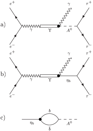
Figure 1: Contributions to $e^{+}e^{-}\to\Upsilon\to\gamma\ \tau^{+}\tau^{-}$ with a) pseudoscalar Higgs, b) $\eta_{b}$, as intermediate states; c) Mixing diagram to be considered in section 4.

For our theoretical estimates we assume that fermions couple to the $A^{0}$ field according to the interaction term

$${\cal L}_{int}^{\bar{f}f}\ =\ -X_{f}\ \frac{A^{0}}{v}m_{f}\bar{f}(i\gamma_{5})f$$ (3)

in the effective Lagrangian, with the vacuum expectation value $v\simeq 246$ GeV; $X_{f}$ depends on the fermion type, whose mass is denoted by $m_{f}$.

Table 1: Measured leptonic branching fractions ${\mathcal{B}[\Upsilon(nS)\to\ell\ell]}$ (in $\%$) and error bars (summed in quadrature) of $\Upsilon(1S)$, $\Upsilon(2S)$ and $\Upsilon(3S)$ resonances (obtained from the PDG [7] and recent CLEO data [28]).

channel:	$e^{+}e^{-}$	$\mu^{+}\mu^{-}$	$\tau^{+}\tau^{-}$	$R_{\tau/\ell}(nS)$
$\Upsilon(1S)$	$2.38\pm 0.11$		$2.61\pm 0.13$	$0.10\pm 0.07$
$\Upsilon(1S)$		$2.48\pm 0.05$	$2.61\pm 0.13$	$0.05\pm 0.06$
$\Upsilon(2S)$	$1.97\pm 0.11$		$2.11\pm 0.15$	$0.07\pm 0.09$
$\Upsilon(2S)$		$1.93\pm 0.17$	$2.11\pm 0.15$	$0.09\pm 0.12$
$\Upsilon(3S)$	$2.18\pm 0.20$		$2.52\pm 0.24$	$0.14\pm 0.14$
$\Upsilon(3S)$		$2.18\pm 0.21$	$2.52\pm 0.24$	$0.14\pm 0.14$

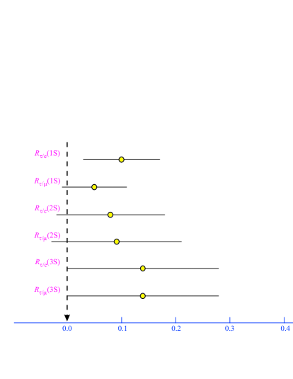
Figure 2: Plot of $R_{\tau/\ell}$ according to Table 1. A small but systematic shift towards positive values can be observed which, however, needs confirmation.

In a 2HDM(II), $X_{d}=\tan{\beta}$ for down-type fermions (where $\tan{\beta}$ stands for the ratio of two Higgs doublet vacuum expectation values) and $X_{u}=\cot{\beta}$ for up-type fermions. Large $\tan{\beta}$ values would imply a large coupling of the $A^{0}$ to the bottom quark but a small coupling to the charm quark, so hereafter we focus on the Upsilon phenomenology.

In the NMSSM, $X_{d}=\cos{\theta_{A}}\tan{\beta}$ where $\theta_{A}$ is the mixing angle between the singlet component (which does not couple to $b\bar{b}$) and the MSSM-like component of the $A^{0}$: $A^{0}=\cos{\theta_{A}}A_{MSSM}+\sin{\theta_{A}}A_{s}$. Notice that for large $\tan{\beta}$, $\cos{\theta_{A}}\sim\sin{2\beta}$ and no further increase of the coupling with $\tan{\beta}$ is expected in this limit. Thus, the constraints on a light CP-odd NMSSM Higgs boson from direct searches at LEP are rather weak.

Experimentally, the relative importance of the postulated NP contribution can be assessed via the ratio of leptonic BF’s

$${\cal R}_{\tau/\ell}=\frac{{\cal B}_{\tau\tau}-{\cal B}_{\ell\ell}}{{\cal B}_{\ell\ell}}=\frac{{\cal B}_{\tau\tau}}{{\cal B}_{\ell\ell}}-1$$ (4)

where ${\cal B}_{\tau\tau}$ denotes the tauonic BF of the $\Upsilon$ resonance and ${\cal B}_{\ell\ell}$, $\ell=e,\mu$ represents either its electronic or muonic BF.

A (statistically significant) non-null value of ${\cal R}_{\tau/\ell}$ would imply the rejection of LU (predicting ${\cal R}_{\tau/\ell}\simeq 0$) and a strong argument supporting the existence of a pseudoscalar Higgs boson mediating the tauonic channel according to the channels of Eqs.(1) and (2). Table 1 shows current experimental data for the $\Upsilon(1S,2S,3S)$ resonances, pointing out the possibility of LU breaking at the $\lesssim 10\%$ level.

2 Non-resonant decay

Soon after the discovery of heavy vector mesons, Wilczek [1] put forward the exciting possibility of finding a light Higgs or an axion through the radiative decay $\Upsilon\to\gamma+H^{0},A^{0}$. The (pseudo)scalar particle could leave the detector volume without decaying inside, or decaying mainly into charmed particles or $\tau^{+}\tau^{-}$ pairs. In either case, an experimental signature was expected to be a rather clean peak in the photon spectrum [6] due to a foreseen small Higgs boson width.

The leading-order expression for the decay width (common to CP-even and -odd particles) reads

$$\Gamma[\Upsilon(nS)\to\gamma A^{0}]=\frac{2\alpha Q_{b}^{2}|R_{n}(0)|^{2}X_{d}^{2}}{v^{2}}\biggl{(}1-\frac{m_{A^{0}}^{2}}{m_{\Upsilon}^{2}}\biggr{)}$$

for $m_{A^{0}}<m_{\Upsilon(nS)}$, where $R_{n}(0)$ and $m_{\Upsilon}$ denote the radial wave function at the origin and mass of the $\Upsilon(nS)$, respectively; $\alpha$ is the fine structure constant and $Q_{b}$ is the electric charge (in units of $|e|$) of the bottom quark. The above width is often divided by the electronic partial width $\Gamma[\Upsilon\to e^{+}e^{-}]$ to obtain the ratio

$$R_{0}=\frac{\Gamma[\Upsilon\to\gamma\ A^{0}]}{\Gamma[\Upsilon\to e^{+}e^{-}]}=\frac{m_{\Upsilon}^{2}\ X_{d}^{2}}{8\pi\alpha\ v^{2}}\biggl{(}1-\frac{m_{A^{0}}^{2}}{m_{\Upsilon}^{2}}\biggr{)}$$ (5)

Strictly speaking, the above formula is only valid when the photon energy is greater than the $\Upsilon$ binding energy. Actually, bound-state effects have a quite different behaviour for a scalar or a pseudoscalar Higgs, reducing the former substantially (even yielding a cancellation at a given boson mass because of the destructive interference of two amplitudes [29]), but increasing $R_{0}$ by $\sim 20\%$ in the latter case [30, 31, 32]. In addition, QCD corrections (at order $\alpha_{s}$) may reduce the ratio $R_{0}$ by a similar amount [33, 34]. Thus the tree-level expression (5) can be used for a pseudoscalar Higgs to an acceptable degree of accuracy.

On the other hand, the decay width of a CP-odd Higgs boson into a tauonic pair is given by

$$\Gamma[A^{0}\rightarrow\tau^{+}\tau^{-}]\simeq\frac{m_{\tau}^{2}X_{d}^{2}}{8\pi v^{2}}\ m_{A^{0}}\ (1-4x_{\tau})^{1/2}$$ (6)

with $x_{\tau}=m_{\tau}^{2}/m_{A^{0}}^{2}$. Next, considering the cascade decay $\Upsilon\to\gamma\ A^{0}(\to\tau^{+}\tau^{-})$ shown in Fig.1.a), and combining Eqs.(5-6) we can write

$${\cal R}_{\tau/\ell}=R_{0}\times\frac{\Gamma[A^{0}\rightarrow\tau^{+}\tau^{-}]}{\Gamma_{A^{0}}}$$ (7)

where $\Gamma_{A^{0}}$ denotes the full width of the pseudocalar Higgs boson. Below open bottom production and above the $\tau^{+}\tau^{-}$ threshold, the tauonic channel should dominate the $A^{0}$ decay even for moderate $X_{d}$, i.e. we can safely set ${\cal B}[A^{0}\to\tau^{+}\tau^{-}]\approx 1$. In section 4, $A^{0}-\eta_{b}$ mixing effects should modify this assumption by changing both the total and partial tauonic decay widths of the $A^{0}$ physical state.

3 Resonant decay

In Ref. [9], use was made of time-ordered perturbation theory to incorporate the effect of intermediate $b\bar{b}$ bound states in the process of Eq.(2) schematically shown in Fig.1.b). We found that the main contribution should come from a $\eta_{b}$ state subsequent to a dipole magnetic (M1) transition of the $\Upsilon$ resonance, in agreement with [32]. Thus, the total decay width can be factorized in the narrow width approximation as [9]

$$\Gamma[\Upsilon\to\gamma\,\ell^{+}\ell^{-}]\ =\ \Gamma^{\,M1}_{\,\Upsilon\to\gamma\eta_{b}}\ \times\ \frac{\Gamma[\eta_{b}\to\ell^{+}\ell^{-}]}{\Gamma_{\eta_{b}}}$$ (8)

where $\Gamma[\eta_{b}\to\ell^{+}\ell^{-}]$ and $\Gamma_{\eta_{b}}$ denote the leptonic width and the total width of the $\eta_{b}$ resonance, respectively; $\Gamma^{\,M1}_{\,\Upsilon\to\gamma\eta_{b}}$ represents the M1 transition width. Next dividing both sides of Eq.(8) by the $\Upsilon$ total width $\Gamma_{\Upsilon}$, we get the cascade decay formula

$${\cal B}[{\,\Upsilon\to\gamma\,\ell^{+}\ell^{-}}]={\cal B}[{\,\Upsilon\to\gamma\eta_{b}}]\times{\cal B}[\eta_{b}\to\ell^{+}\ell^{-}]$$

The BF for a M1 transition between $\Upsilon(nS)$ and $\eta_{b}(n^{\prime})$ states ($n^{\prime}\leq n$) is given by [38]

$${\cal B}[\Upsilon(nS)\to\gamma\eta_{b}(n^{\prime}S)]=\frac{16\alpha}{3}\biggl{(}\frac{Q_{b}}{2m_{b}}\biggr{)}^{2}\ \frac{I^{2}\cdot k^{3}}{\Gamma_{\Upsilon}}$$ (9)

where $k$ is the photon energy (approximately equal to the mass difference $m_{\Upsilon(nS)}-m_{\eta_{b}(n^{\prime}S)}$); $I$ represents the initial and final wave functions overlap, $\langle f|j_{0}(kr/2)|i\rangle$, where $j_{0}$ is a spherical Bessel function. $I$ is numerically close to unity for favored transitions ($n=n^{\prime}$) but much smaller for hindered ($n\neq n^{\prime}$) transitions. As stressed in [38], however, the considerably larger photon energy $k$ in the latter case could compensate this drawback, leading to competitive transition probabilities. Therefore $\Upsilon(2S)$ and $\Upsilon(3S)$ hindered transitions into $\eta_{b}(2S)$ and $\eta_{b}(1S)$ states have to be taken into account as potential contributions to the process of Eq.(2).

The $A^{0}$-mediated decay width of the $\eta_{b}$ into $\tau^{+}\tau^{-}$ can be related to the electromagnetic decay of the Upsilon resonance as [9]

$$\frac{\Gamma[\eta_{b}\to\tau^{+}\tau^{-}]}{\Gamma[\Upsilon\to e^{+}e^{-}]}\simeq\frac{3m_{b}^{4}m_{\tau}^{2}(1-4x_{\tau})^{1/2}X_{d}^{4}}{32\pi^{2}Q_{b}^{2}\alpha^{2}\Delta M^{2}v^{4}}$$

where now $x_{\tau}=m_{\tau}^{2}/m_{\eta_{b}}^{2}$, $\Delta M=|m_{A^{0}}-m_{\eta_{b}}|$ and the $A^{0}$ width was neglected. Note again that the NP contribution to the $\Upsilon$ leptonic decay would be significant only for the tauonic mode. Finally one gets for the ratio (4)

$${\cal R}_{\tau/\ell}\simeq\biggl{[}\frac{m_{b}^{2}m_{\tau}^{2}(1-4x_{\tau})^{1/2}}{8\pi^{2}{\alpha}v^{4}}\biggr{]}\times\frac{I^{2}\ k^{3}X_{d}^{4}}{\Gamma_{\eta_{b}}{\Delta}M^{2}}$$ (10)

In order to crudely estimate $\Gamma_{\eta_{b}}$, we can employ the asymptotic pQCD expression [39]

$$\frac{\Gamma_{\eta_{b}}}{\Gamma_{\eta_{c}}}\simeq\frac{m_{b}}{m_{c}}\times\biggl{[}\frac{\alpha_{s}(\mu_{b})}{\alpha_{s}(\mu_{c})}\biggr{]}^{5}$$

Setting $m_{b}=4.7$ GeV, $m_{c}=1.5$ GeV, $\Gamma_{\eta_{c}}=25.5\pm 3.4$ MeV [7] and varying the scales $\mu_{c}$ ($\mu_{b}$) between $m_{c}$ and $2m_{c}$ ($m_{b}$ and $2m_{b}$), one gets $\Gamma_{\eta_{b}}\simeq\Gamma[\eta_{b}\to gg]\sim 5-10$ MeV although with a large uncertainty. Let us remark that a large $\eta_{b}$ hadronic decay width (i.e. $\Gamma[\eta_{b}\to gg]>10$ MeV) would damp resonant effects in the process (2), as can be seen from Eq.(8).

For large enough $X_{d}$, the tauonic decay mode of the $\eta_{b}$ becomes comparable to the hadronic mode provided by the 2 gluon channel (even becoming dominant for $X_{d}\gtrsim 25$), i.e. $\Gamma[\eta_{b}\to\tau^{+}\tau^{-}]\gtrsim\Gamma[{\eta_{b}}\to gg]\$; thus ${\cal B}[\eta_{b}\to\tau^{+}\tau^{-}]\simeq 50-100\%$ and

$${\cal R}_{\tau/\ell}\simeq\frac{{\cal B}[\Upsilon\to\gamma\eta_{b}]}{{\cal B}_{\ell\ell}}\ \simeq\ 1-10\ \%$$

using different values of ${\cal B}[\Upsilon\to\gamma\eta_{b}]$ summarized in Ref. [38]. A similar result will be obtained in the next section employing the mixing formalism.

4 Mixing

So far we have neglected the widths of both $\eta_{b}$ and $A^{0}$ in the theoretical calculation of the ratio (4). However, for a light Higgs boson it may happen that the $\eta_{b}$ and $A^{0}$ masses are close, e.g. within several $\Gamma_{\eta_{b}}$, $\Gamma_{A^{0}}$. Then, a significant mixing between the pseudoscalar resonance and a CP-odd Higgs boson should occur, modifying the naive estimates of (7) and (10). Throughout we will consider the simplified situation where the light Higgs mixes appreciably with only one $\eta_{b}$ state, notably the $\eta_{b}(1S)$ resonance.

The mixing between Higgs and resonances is described by the introduction of off-diagonal elements denoted by $\delta m^{2}$ in the mass matrix [35, 27]

$${\cal M}_{0}^{2}=\left(\begin{array}[]{cc}m_{A_{0}^{0}}^{2}-im_{A_{0}^{0}}\Gamma_{A_{0}^{0}}&\delta m^{2}\\ \delta m^{2}&m_{\eta_{b0}}^{2}-im_{\eta_{b0}}\Gamma_{\eta_{b0}}\end{array}\right)$$

where the subindex $`$0’ indicates unmixed states. The off-diagonal element $\delta m^{2}$ can be computed (see Fig.1.c) within the framework of a nonrelativistic quark potential model. For the pseudoscalar case under study, one can write

$$\delta m^{2}\ =\ \biggl{(}\frac{3m_{\eta_{b}}^{3}}{4\pi v^{2}}\biggr{)}^{1/2}|R_{\eta_{b}}(0)|\times X_{d}\$$ (11)

Notice that $\delta m^{2}$ is proportional to $X_{d}$; substituting numerical values (for the radial wave function at the origin we use the potential model estimate $|R_{\eta_{b}}(0)|^{2}=$ 6.5 GeV³ from [36]) one finds: $\delta m^{2}$(GeV²) $\approx\ 0.146\ \times\ X_{d}$.

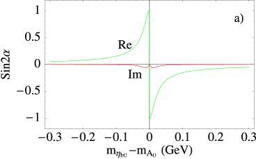
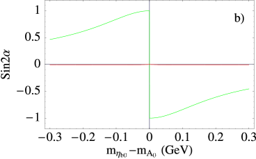
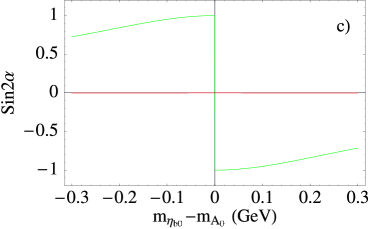
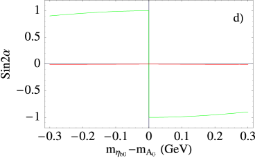
Figure 3: $\sin{2\alpha}$ versus the mass difference of the unmixed states setting $m_{\eta_{b0}}=9.3$ GeV and $\Gamma_{\eta_{b0}}=5$ MeV, for: $a)$ $X_{d}=1$ (Fig.2 of Ref. [27] is recovered); $b),c),d)$ $X_{d}=10,20,40$, respectively. Solid (green) line: real part, dotted (red) line: imaginary part. The change of sign of the real part is a consequence of the definition of the mixing angle between the $A^{0}$ and $A_{0}^{0}$ states. The imaginary part is negligible in our numerical computations and the normalization $N$ of mixed states is near unity.

Now defining $\Delta^{2}=[D^{2}+(\delta m^{2})^{2}]^{1/2}$, where $D=(m_{A_{0}^{0}}^{2}-m_{\eta_{b0}}^{2}-im_{A_{0}^{0}}\Gamma_{A_{0}^{0}}+im_{\eta_{b0}}\Gamma_{\eta_{b0}})/2$, the mixing angle $\alpha$ between the physical Higgs $A^{0}$ and the unmixed $A_{0}^{0}$ can be defined through

$$\sin{}2\alpha\ =\ \delta m^{2}/\Delta^{2}$$ (12)

giving rise to the physical eigenstates:

$$A^{0} = \frac{1}{N}\{\cos{\alpha}\ A_{0}^{0}\ +\ \sin{\alpha}\ \eta_{b0}\}$$

$$\eta_{b} = \frac{1}{N}\{\cos{\alpha}\ \eta_{b0}\ -\ \sin{\alpha}\ A_{0}^{0}\}$$

where $N=\{|\cos{\alpha}|^{2}+|\sin{\alpha}|^{2}\}^{1/2}$, which can be different from unity since the mixing angle is in general complex, although we can set $N\simeq 1$ in our calculations.

Fig.3 shows $\sin{2\alpha}$ as a function of the $\eta_{b0}$ and $A_{0}^{0}$ mass difference for $X_{d}=1,10,20,40$ and $\Gamma_{\eta_{b0}}=5$ MeV. Note that mixing effects can be important over a large mass region (i.e. several hundreds of MeV), especially for large $X_{d}$ values.

On the other hand, the couplings of the physical $A^{0}$ and $\eta_{b}$ states to a $\tau^{+}\tau^{-}$ pair are given by

$$g_{A^{0}\tau\tau} = \frac{1}{N}\{\cos{\alpha}\ g_{A_{0}^{0}\tau\tau}\ +\ \sin{\alpha}\ g_{\eta_{b0}\tau\tau}\}$$

$$g_{\eta_{b}\tau\tau} = \frac{1}{N}\{\cos{\alpha}\ g_{\eta_{b0}\tau\tau}\ -\ \sin{\alpha}\ g_{A_{0}^{0}\tau\tau}\}$$

In the SM we can very approximately set $g_{\eta_{b0}\tau\tau}\simeq 0$ and thus write

$$g_{A^{0}\tau\tau}\simeq g_{A_{0}^{0}\tau\tau}\cos{\alpha},\ g_{\eta_{b}\tau\tau}\simeq-g_{A_{0}^{0}\tau\tau}\sin{\alpha}$$ (13)

where $g_{A_{0}^{0}\tau\tau}$ can be obtained from the Yukawa coupling strength provided by Eq.(3). We should emphasize that, in order to account for the decay $\Upsilon\to\gamma\ \tau^{+}\tau^{-}$, both channels represented in Eqs.(1) and (2) have to be considered altogether, taking into account the mixing diagram of Fig.1.c) and modifying the tauonic couplings accordingly.

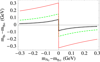
Figure 4: Shift of the $\eta_{b}$ physical mass induced by its mixing with a pseudoscalar Higgs boson, versus $m_{A_{0}^{0}}-m_{\eta_{b0}}$ for: dotted (black) line: $X_{d}=10$, dashed (green) line: $X_{d}=20$, solid (red) line: $X_{d}=40$. The mass of the $\eta_{b}$ mixed state is decreased (increased) if $m_{A_{0}^{0}}>m_{\eta_{b0}}$ ($m_{A_{0}^{0}}<m_{\eta_{b0}}$), ultimately implying a larger (smaller) $\Upsilon-\eta_{b}$ mass splitting than expected in the SM.

Now, introducing the complex quantity $E=m_{A_{0}^{0}}^{2}+m_{\eta_{b0}}^{2}-im_{\eta_{b0}}\Gamma_{\eta_{b0}}-im_{A_{0}^{0}}\Gamma_{A_{0}^{0}}$, the masses and decay widths of the mixed (physical) states are given by

$$m_{1,2}^{2}-im_{1,2}\Gamma_{1,2}=\frac{E}{2}\ {\pm}\ \Delta^{2}$$ (14)

where subscripts $1,2$ refer to a Higgs-like state and a resonance-like state respectively, if $m_{A_{0}^{0}}>m_{\eta_{b0}}$, and the converse if $m_{A_{0}^{0}}<m_{\eta_{b0}}$. The real (imaginary) part of the r.h.s. of Eq.(14) provides the masses (widths) of the $A^{0}$ and $\eta_{b}$ physical states.

Moreover, the full widths $\Gamma_{A^{0}}$ and $\Gamma_{\eta_{b}}$ of the physical states can be expressed in terms of the widths of the unmixed states according to the simple formulae:

$$\Gamma_{A^{0}} \simeq |\cos{\alpha}|^{2}\ \Gamma_{A_{0}^{0}}\ +\ |\sin{\alpha}|^{2}\ \Gamma_{\eta_{b0}}$$ (15)

$$\Gamma_{\eta_{b}} \simeq |\cos{\alpha}|^{2}\ \Gamma_{\eta_{b0}}\ +\ |\sin{\alpha}|^{2}\ \Gamma_{A_{0}^{0}}$$ (16)

Notice that $\Gamma_{\eta_{b0}}>>\Gamma_{A^{0}_{0}}$ was generally assumed in Ref. [27], while in this work both $\eta_{b0}$ and $A_{0}^{0}$ widths can be comparable (the latter grows as $X_{d}^{2}$). In particular, for large $\delta m^{2}$, $\sin{2\alpha}\simeq 1$ at $m_{A_{0}^{0}}=m_{\eta_{b0}}$ and thus $\Gamma_{\eta_{b}}\simeq\Gamma_{A^{0}}\simeq(\Gamma_{\eta_{b0}}+\Gamma_{A^{0}_{0}})/2$.

In addition, spectroscopic effects can appear in $b\bar{b}(^{1}S_{0})$ states if the $A^{0}_{0}-\eta_{b0}$ mixing sizeably shifts the masses of the physical states. In Fig. 4 we plot $m_{\eta_{b}(1S)}-m_{\eta_{b0}(1S)}$ versus $m_{A_{0}^{0}}-m_{\eta_{b0}}$. Such a shift has to be added (with its sign) to the QCD expected $m_{\Upsilon(1S)}-m_{\eta_{b}(1S)}$ hyperfine splitting, whose theoretical prediction is achieving a remarkable precision [37]. As a consequence, if $m_{\eta_{b0}}<m_{A_{0}^{0}}$, the hyperfine splitting could considerably increase with respect to the SM expectations even at moderate $X_{d}$ values. Let us remark that, in this case, the energy $k$ of the radiated photon could reach values well above 100 MeV in the $\Upsilon(1S)\to\eta_{b}(1S)$ M1 transition, substantially raising the rate due to the $k^{3}$ dependence.

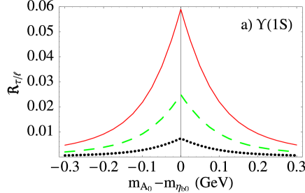
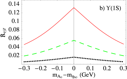
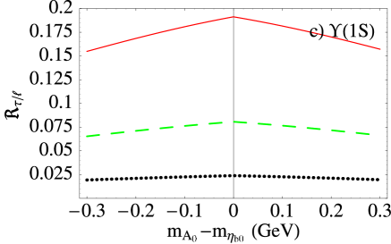
Figure 5: $R_{\tau/\ell}$ from Eq.(18) (resonant production) versus the mass difference of the unmixed states for: $\Upsilon(1)$ with $X_{d}=$ $a)$ 10, $b)$ 20, $c)$ 40, respectively. In each plot, $k=100$ MeV (dotted black line), $k=150$ MeV (dashed green line) and $k=200$ MeV (solid red line).

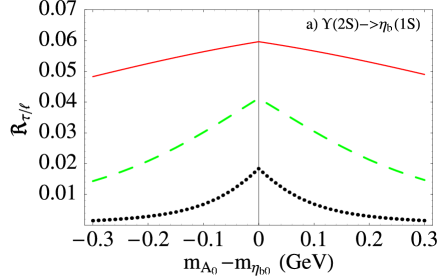
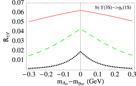
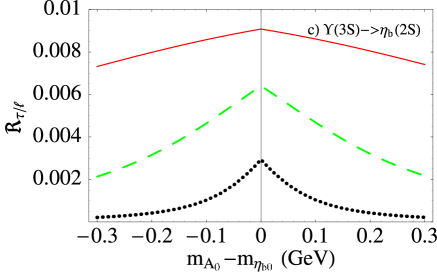
Figure 6: $R_{\tau/\ell}$ from Eq.(18) (resonant production) versus the mass difference of the unmixed states for: $a)$ $\Upsilon(2S)\to\gamma\eta_{b}(1S)$, $b)$ $\Upsilon(3S)\to\gamma\eta_{b}(1S)$, and c) $\Upsilon(3S)\to\gamma\eta_{b}(2S)$, respectively. We set $m_{\eta_{b}(1S,2S)}=9.3$, 9.96 GeV, $X_{d}=10$ (dotted black line), 20 (dashed green line) and 40 (solid red line).

5 Numerical Analysis

The ultimate goal of this study is to evaluate the level of LU breaking in $\Upsilon$ decays due to the NP contribution when mixing effects are taken into account. To this end, we ought to modify the expressions (7) and (10) of $R_{\tau/\ell}$ corresponding to non-resonant and resonant contributions to the decay, by changing the widths in accordance with Eqs.(15-16). Hence Eq.(7) becomes

$${\cal R}_{\tau/\ell}=R_{0}\times\frac{|\cos{\alpha}|^{2}\ \Gamma[A_{0}^{0}\rightarrow\tau^{+}\tau^{-}]}{|\cos{\alpha}|^{2}\Gamma_{A_{0}^{0}}+|\sin{\alpha}|^{2}\Gamma_{\eta_{b0}}}$$ (17)

where $\alpha$ depends on the masses of the unmixed states $A_{0}^{0}$ and $\eta_{b0}$ following (12). The corresponding formula for resonant production using the mixing formalism can be written as

$$R_{\tau/\ell}=\frac{{\cal B}[\Upsilon\to\gamma\eta_{b}]}{{\cal B}_{\ell\ell}}\cdot\frac{|\sin{\alpha}|^{2}\Gamma[A_{0}^{0}\to\tau^{+}\tau^{-}]}{|\cos{\alpha}|^{2}\Gamma_{\eta_{b0}}+|\sin{\alpha}|^{2}\Gamma_{A_{0}^{0}}}$$ (18)

The above expression results in Eq.(10) for small mixing angles, as can be verified using Eqs.(9-12) for $|m_{\eta_{b}}-m_{A^{0}}|>\Gamma_{A^{0}},\Gamma_{\eta_{b}}$, under the approximation $m_{\Upsilon}\simeq m_{\eta_{b}}\simeq 2m_{b}$.

From an experimental viewpoint, both statistical and systematic uncertainties in the $R_{\tau/\ell}$ measurement were estimated to be of order of the few percent level in a proposal for testing LU at a (Super) B factory [8]. Due to the high-luminosity of the machine, the actual limitation for the measurement accuracy should come from the systematic error, expected to be $\lesssim 3.7\%$, representing a reference value for the observability of NP effects in LU analyses.

In Fig.5 we plot $R_{\tau/\ell}$ versus $m_{A_{0}^{0}}-m_{\eta_{b0}}$ for the $\Upsilon(1S)$ resonant decay via an intermediate $\eta_{b}(1S)$ state, using $X_{d}=10,20,40$ and $k=100,150,200$ MeV. Observable effects only become likely for $X_{d}\gtrsim 10$ and $k\gtrsim 150$ MeV. This requirement implies a hyperfine splitting $\Upsilon(1S)$-$\eta_{b}(1S)$ larger than expected in the SM but made possible by the mixing as shown in Fig.4.

Figs. 6.a) and b) show $R_{\tau/\ell}$ for $\Upsilon(2S,3S)$ resonant decays via an intermediate $\eta_{b}(1S)$ state, versus $m_{A_{0}^{0}}-m_{\eta_{b0}}$ for $X_{d}=10,20,40$, setting $I=0.057,0.029$ as overlap factors respectively [38]. In Fig.6.c) we plot $R_{\tau/\ell}$ for $\Upsilon(3S)$ resonant decays via a $\eta_{b}(2S)$ state for $k=400$ MeV and $I=0.054$ [38]. The latter decay is significantly more suppressed than the former two and will be ignored. A caveat is in order. All these rates depend strongly on $I$ and $\Gamma_{\eta_{b0}}$, both quite uncertain.

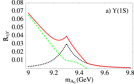
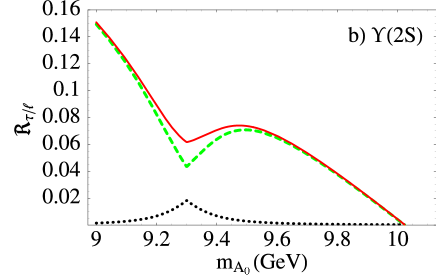
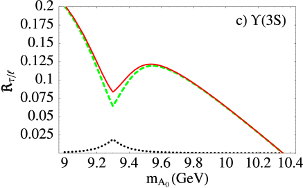
Figure 7: $R_{\tau/\ell}$ versus the pseudoscalar Higgs mass for $a)$ $\Upsilon(1S)$, $b)$ $\Upsilon(2S)$, and $c)$ $\Upsilon(3S)$ decays using $X_{d}=10$, $m_{\eta_{b0}}=9.3$ GeV, and $\Gamma_{\eta_{b0}}=5$ MeV, respectively. Resonant (dotted black line) and non-resonant (dashed green line) decays are added in the solid red line. The non-resonant contribution is shaped by the $|\cos{\alpha}|^{2}$ dependence of the $A^{0}$ partial decay width in Eq.(17), due to the mixing with the pseudoscalar resonance, and the variation of the $A^{0}$ full width. Larger (smaller) values of $X_{d}$ obviously yield higher (lower) expectations for $R_{\tau/\ell}$.

In Figures 7 we plot altogether resonant and non-resonant decays for the $\Upsilon(1S,2S,3S)$ resonances with $\Gamma_{\eta_{b0}}$=5 MeV and $X_{d}$=10 as reference values. According to the NMSSM, $X_{d}=\cos{\theta_{A}}\tan{\beta}$, where $\cos{\theta_{A}}$ is expected typically small [17], i.e. $\cos{\theta_{A}}\sim few\times 10^{-1}$. Therefore $X_{d}=10$ implies $\tan{\beta}\sim several\times 10$. Furthermore, note that in models other than the NMSSM, the singlet $A^{0}$ component might not need to be so large and, consequently, $\cos{\theta_{A}}$ could be not so small, making larger $X_{d}$ plausible while keeping reasonable $\tan{\beta}$ values.

The set of plots of Fig.7 constitute our main result from which we draw the final conclusions. By inspection, a bump can be seen in Fig.7.a) due to the resonant contribution, while a dip appears in Figs.7.b) and c) on account of the suppressed non-resonant channel, not compensated by the resonant channel. In spite of that, the higher values of $R_{\tau/\ell}$ obtained in the two latter cases allow us to conclude that $\Upsilon(2S,3S)$ radiative decays look more promising than the $\Upsilon(1S)$ decays for the experimental observation of LU breaking at the few percent level. This conclusion is important if a specific test of LU were to be put forward by experimental collaborations.

6 Summary

Lepton universality breaking in $\Upsilon$ decays could be a harbinger of new physics, in particular of a light CP-odd non-standard Higgs boson. In this paper, we have studied non-resonant and resonant $\Upsilon$ decays taking into account $A^{0}-\eta_{b}$ mixing effects, concluding that, for this particular goal of testing LU, $\Upsilon(2S,3S)$ radiative decays look more promising than the $\Upsilon(1S)$ decay. Moreover, the discovery of $\eta_{b}$ states and a light CP-odd Higgs boson would become both experimentally and theoretically entangled. Indeed, the observation of a large tauonic BF of any $\eta_{b}$ state could be related to the existence of a light Higgs boson. In addition, unexpectedly large hyperfine splittings in the bottomonium family would also be another hint of new physics.

High luminosity (Super) B factories should play a crucial role for testing LU in $\Upsilon$ decays (perhaps below the few percent level if systematics are well under control) in the quest for new physics at this energy scale.

Acknowledgements We gratefully acknowledge J. Bernabeu, N. Brambilla, F.J. Botella, J. Papavassiliou and A. Vairo for useful discussions. M.A.S.L. thanks R. Dermisek, G. Faldt, J. Gunion, B. McElrath, P. Osland and T. T. Wu for valuable exchange of emails.

References

- [1] F. Wilczek, Phys. Rev. Lett. 40 (1978) 279.
- [2] H. E. Haber, G. L. Kane and T. Sterling, Nucl. Phys. B 161 (1979) 493.
- [3] J. R. Ellis, M. K. Gaillard, D. V. Nanopoulos and C. T. Sachrajda, Phys. Lett. B 83 (1979) 339.
- [4] C. Peck et al. [Crystal Ball Collaboration], SLAC-PUB-3380.
- [5] D. Besson et al. [CLEO Collaboration], Phys. Rev. D 33 (1986) 300.
- [6] H. Albrecht et al. [ARGUS Collaboration], Phys. Lett. B 154 (1985) 452.
- [7] W. M. Yao et al. [Particle Data Group], J. Phys. G 33 (2006) 1.
- [8] M. A. Sanchis-Lozano, arXiv:hep-ph/0610046.
- [9] M. A. Sanchis-Lozano, Int. J. Mod. Phys. A 19 (2004) 2183.
- [10] J. F. Gunion, H. E. Haber, G. Kane and S. Dawson, The Higgs Hunter’s Guide (Addison-Wesley Publishing Company, Redwood City, CA, 1990).
- [11] B. A. Dobrescu and K. T. Matchev, JHEP 0009, 031 (2000).
- [12] G. Hiller, Phys. Rev. D 70, 034018 (2004).
- [13] R. Dermisek and J. F. Gunion, Phys. Rev. Lett. 95 (2005) 041801.
- [14] R. Dermisek and J. F. Gunion, Phys. Rev. D 73 (2006) 111701.
- [15] J. F. Gunion, D. Hooper and B. McElrath, Phys. Rev. D 73 (2006) 015011.
- [16] B. McElrath, Phys. Rev. D 72, 103508 (2005).
- [17] R. Dermisek, J. F. Gunion and B. McElrath, arXiv:hep-ph/0612031.
- [18] T. Han, P. Langacker and B. McElrath, Phys. Rev. D 70 (2004) 115006.
- [19] M. Carena, J. R. Ellis, S. Mrenna, A. Pilaftsis and C. E. M. Wagner, Nucl. Phys. B 659 (2003) 145.
- [20] S. Kraml et al., arXiv:hep-ph/0608079.
- [21] S. Schael et al. [ALEPH Collaboration], Eur. Phys. J. C 47 (2006) 547.
- [22] G. Abbiendi et al. [OPAL Collaboration], Eur. Phys. J. C 40 (2005) 317.
- [23] G. W. Bennett et al. [Muon G-2 Collaboration], Phys. Rev. D 73 (2006) 072003.
- [24] M. Krawczyk, arXiv:hep-ph/0103223.
- [25] K. Hagiwara, A. D. Martin, D. Nomura and T. Teubner, arXiv:hep-ph/0611102.
- [26] M. A. Sanchis-Lozano, PoS HEP2005 (2006) 334.
- [27] M. Drees and K. i. Hikasa, Phys. Rev. D 41, 1547 (1990).
- [28] D. Besson [CLEO Collaboration], Phys. Rev. Lett. 98 (2007) 052002 [arXiv:hep-ex/0607019].
- [29] G. Faldt, P. Osland and T. T. Wu, Phys. Rev. D 38 (1988) 164.
- [30] J. Polchinski, S. R. Sharpe and T. Barnes, Phys. Lett. B 148 (1984) 493.
- [31] J. T. Pantaleone, M. E. Peskin and S. H. H. Tye, Phys. Lett. B 149 (1984) 225.
- [32] W. Bernreuther and W. Wetzel, Z. Phys. C 30 (1986) 421.
- [33] M. I. Vysotsky, Phys. Lett. B 97 (1980) 159.
- [34] P. Nason, Phys. Lett. B 175 (1986) 223.
- [35] P. J. Franzini and F. J. Gilman, Phys. Rev. D 32 (1985) 237.
- [36] E. J. Eichten and C. Quigg, Phys. Rev. D 52 (1995) 1726 [arXiv:hep-ph/9503356].
- [37] N. Brambilla et al., arXiv:hep-ph/0412158.
- [38] S. Godfrey and J. L. Rosner, Phys. Rev. D 64 (2001) 074011 [Erratum-ibid. D 65 (2002) 039901].
- [39] A. Le Yaouanc et al., Hadron transitions in the quark model (Gordon and Breach Science Publishers, 1988).