Heavy baryons in the Skyrme model: the role of highly anharmonic collective motion

Abstract

In the heavy quark and large $N_{c}$ limits, ordinary (exotic) heavy baryons can be considered as bound states of heavy mesons (anti-mesons)and chiral solitons. In these limits, the heavy mesons (or anti-mesons) and the chiral solitons are extremely heavy and are presumed to fall to the bottom of the effective potential. Previous studies have approximated the effective potential as harmonic about the minimum. However, when realistic masses for the heavy meson and chiral soliton are considered, longer range parts of the effective potential can become relevant. In this paper, we show that these longer-ranged effects yield effective wave functions which are qualitatively very different from those expected from the combined large $N_{c}$ and heavy quark limits. These potentials can support bound heavy pentaquarks under some conditions. The consequence of these new energy states and wave functions on the Isgur-Wise function for the semileptonic decay of heavy baryons is also considered.

I Introduction

It has been known for a number of years that heavy baryons can be constructed in the heavy quark and large $N_{c}$ limits from the binding of heavy mesons with light chiral solitons jmw ; glm ; jm ; ck1 ; ck2 . In these limits, both the heavy meson and the chiral soliton have large masses, and it is legitimate to describe the system in terms of a collective degree of freedom between the heavy meson and baryon. The large masses drive the particles to the bottom of the effective potential. In most cases considered, this minimum occurs at the origin of the relative coordinate, causing both particles to be situated on top of one another. Previous attempts at describing heavy baryon physics within this model assumed that particles would only experience small harmonic perturbations in the potential away from their minimum. The previous works showed that the channels which constituted physical heavy baryons had attractive potentials while those channels which did not correspond to physical particles had repulsive potentials jmw ; glm ; jm . Since the physical world does not correspond to the extreme heavy quark and large $N_{c}$ limits, which guided the previous work, it is interesting to ask the extent to which realistic masses drive the particles to the bottom of the potential (as expected in the combined limit) when the harmonic approximation to the effective potential is replaced by the leading order potential to all distances. In this paper, we look at a class of corrections to this picture. Similar issues have arisen for nucleon-nucleon forces in large $N_{c}$ boris . We continue to assume that the heavy quark mass and $N_{c}$ are large enough to enable us to describe the dynamics in terms of a collective degree of freedom which is describable as a non-relativistic effective potential. However, we do not automatically assume that the masses are so large as to drive the particles into the vicinity of the the minimum of the potential. Instead, we focus on examining the consequences of considering the complete potential with realistic particle masses on heavy baryon physics. As we will show, the physics is qualitatively quite different from what one would expect if the world were close to the idealized limit.

Baryons described as solitons in a chiral Lagrangian were first considered by Skyrme skyrme . These chiral solitons have the correct quantum numbers as baryons in the large $N_{c}$ limit witten when the Wess-Zumino term is included wz . While the extensive early calculations anw focused on $SU(2)$ solitons, the theory was also extended to include baryons with strange quarks. This was done by either considering the strange quark as light, and extending the $SU(2)$ chiral fields to $SU(3)$ guadagnini ; manohar , or by considering the strange quarks as heavy, compared to the lighter quarks, and strange baryons as bound states of the $SU(2)$ soltion and K-mesons callan1 ; callan2 .

To extend the theory to include even heavier quarks, such as charm and bottom, the former approach of extending the soliton group structure is not reasonable since the mass of the heavy quarks is vastly different from the lighter three quarks. Therefore, the appropriate manner is the latter, put forth in the strange case by Callan and Klebanov, where the heavy baryon states are considered bound states of light quark chiral solitons and heavy mesons. For simplification, we will focus our attention on models made from $SU(2)$ chiral solitons, as was done in previous work jmw ; glm ; jm . Furthermore, the theory must also exhibit heavy quark symmetrywise ; bd ; yan . Thereby, the heavy meson is treated by heavy quark effective theory (HQET). HQET treats the heavy mesons as the dynamical degrees of freedom and provides a systematic expansion, in powers of the hadronic scale, $\Lambda$, over the heavy quark mass, $m_{Q}$, to examine the Lagrangian and subsequent interactions.

This method can also be used to bind heavy anti-mesons with chiral solitons to form pentaquark states. Such calculations have been performed previously, for the case of strange quarks klebanov . This work showed that the pentaquark channel was not sufficiently attractive to yield bound pentaquark states or prominent resonances. Previously, it has been argued on general model-independent grounds that in the extreme heavy quark and large $N_{c}$ limits, bound heavy pentaquark states must exist, primarily because the heavy particles fall to the bottom of the potential well hohler1 . However, it was shown that unlike in the extreme heavy quark and large $N_{c}$ limits in which the long-range one-pion-exchange potential automatically binds heavy pentaquarks regardless of the details of the short distance interactions, for physical masses the existence of bound pentaquarks was highly sensitive to the details of the short distance interaction. The Skyrme type chiral soliton models provide one framework for treating the short distance physics, and thereby it is interesting to determine if such theories could support heavy pentaquark binding. More significantly, the experience with the exotic channels suggests the possibility that the behavior in the non-exotic channels may also be substantially different from the limit on which the standard Skyrme analysis is based.

The interest in determining the heavy baryon energy spectrum and wave function within a chiral soliton model has also led to studies of the Isgur-Wise function for transitions between heavy baryons. Formally, the Isgur-Wise function describes the non-perturbative physics associated with the form factor of the semileptonic weak decay of $\Lambda_{b}\rightarrow\Lambda_{c}e^{-}\bar{\nu}_{e}$ isgurwise . Traditionally is is expressed as a function of the transition velocity. If the dynamics of the heavy baryons are known exactly, this function can be calculated for all velocities. The Isgur-Wise function has been calculated previously when the effective potential was approximated as harmonic both in the context of the Skyrme modeljm and in a model-independent contextck1 ; ck2 . This paper considers the longer range effects of the interaction between the heavy and light degrees of freedom and leads to a non-universal form of the Isgur-Wise function dependent on the details of the interaction.

We are by no means the first group to consider applying the Skyrme model to attempt to explain either heavy baryons or exotic particles. In addition to jmw ; glm ; jm , heavy baryons spectroscopy within the Skyrme model has been previous considered by the work of Oh and his collaborators oh . In recent years, a variety of work associated with pentaquarks states has been presented in the literature. These works have included heavy pentaquarks, in the context of several different models, hohler1 ; wessling1 ; wessling ; stancu , and light pentaquark states either in the context of the Skyrme model, diakonov ; walliser ; cohen2 ; cherman ; trampetic1 , or in terms of other models, jaffe ; kopelovich ; lipkin ; cohen3 . Exoctic dibaryon states have also been examined using the Skyrme model balachandran . Additionally, decays of heavy baryons have been previously considered within the Skyrme model, trampetic2 .

The overall goal of this paper is to explore the properties of heavy baryons in the Skyrme model in which the collective degree of freedom between the heavy meson and the remainder of the system is beyond the harmonic region of the ideal heavy quark and large $N_{c}$ limits. In the next section, we derive the complete effective potential and show that when the full potential is considered, for realistic parameters, the heavy baryon wave function extends well beyond the region where the harmonic approximation is applicable. This will be followed by a demonstration that the simplest type of interactions do not create bound states with realistic binding energies for the heavy baryons—indeed they give the same mass for ordinary heavy baryons and pentaquarks. This motivates the inclusion of additional terms in the potential terms which allow for the correct binding energies and distinguish between heavy baryon and heavy pentaquark states. The consequences of these new potentials will be considered. Lastly, we will examine how these newly calculated wave functions for the heavy baryons influences the Isgur-Wise function.

II Derivation of the effective potential

The framework of this paper is based on the standard treatment of heavy baryons in the Skyrmion in terms of a collective degree of freedom between the heavy meson and the remainder of the system jmw ; glm ; jm . To begin the analysis of heavy baryons, the effective potential for this degree of freedom needs to be determined. The relevant Lagrangian for this purpose can be divided into the soliton sector and the HQET sector,

$$\mathcal{L}=\mathcal{L_{\text{Skyrme}}}+\mathcal{L_{\text{HQET}}}.$$ (1)

The soliton portion determines the dynamics of the ordinary baryons. For concreteness we will consider the simplest such model; the one originally proposed by Skyrme:

$$\mathcal{L_{\text{Skyrme}}}=\frac{1}{16}\,f_{\pi}^{2}\,\text{Tr}[\partial_{\mu}\Sigma^{\dagger}\partial^{\mu}\Sigma]+\frac{1}{32e^{2}}\,\text{Tr}[(\partial_{\mu}\Sigma)\Sigma^{\dagger},(\partial_{\nu}\Sigma)\Sigma^{\dagger}]^{2}+\frac{1}{8}\,m_{\pi}^{2}f_{\pi}^{2}\,(\text{Tr}[\Sigma]-2),$$ (2)

where $f_{\pi}$ is the pion decay constant, $e$ is the Skyrme parameter, $m_{\pi}$ is the pion mass, and $\Sigma$ is the chiral soliton field skyrme . The last term provides the pion with a mass and fixes it to its physical value. As we will see below, this simplest model is not adequate phenomenologically. However, we will begin with an analysis of this model and consider more sophisticated models subsequently.

Conventionally, the chiral soliton is treated classically as a first approximation and the ansatz taken for the form of the chiral field is,

$$\Sigma_{0}(\vec{x})=\text{Exp}[i\vec{\tau}\cdot\hat{x}\;F(r)],$$ (3)

where $F(r)$ is the profile function determined by minimization of the soliton mass. Since this solution breaks both rotational and isorational invariance, any rotation within the isospin space will lead to a degenerate classical solution. That is,

$$\Sigma(\vec{x})=A\,\Sigma_{0}(\vec{x})\,A^{-1}$$ (4)

where $A$ is an $SU(2)$ matrix of the form $A=a_{0}+i\vec{\tau}\cdot\vec{a}$ where $a_{0}$ and $\vec{a}$ (with $a_{0}^{2}+\vec{a}\cdot\vec{a}=1$) leads to a degenerate solution. This classical degeneracy is lifted when $a_{0}$ and $\vec{a}$ are promoted to quantum collective variables leading to baryons with the physical quantum numbersanw .

However, there is a subtlety concerning the use of the quantization scheme of ANW for the regime considered here. There are two types of collective motion—the rotational/isorotational degrees of freedom of ANW and the collective vibration of the heavy meson off of the baryon. Provided that the natural time scales for these types of motion are very different they decouple. Formally, in the large $N_{c}$ and heavy quark limits, when the collective vibrational degree of freedom resides near the bottom of the potential well and vibrates harmonically its natural time scale goes as $\lambda^{-1/2}$ ck3 while the time scale of the ANW collective coordinate is $\lambda^{-1}$, where $\lambda$ is an overall counting parameter for the combined limit:

$$\frac{1}{N_{c}}\sim\frac{M_{H}}{\Lambda}\sim\lambda$$ (5)

where $\Lambda$ is the characteristic hadron mass scale. Formally, in the ideal limit, $\lambda\rightarrow 0$ and the two scales decouple. However, in the present study where we are explicitly looking for effects beyond the $\lambda\rightarrow 0$ limit the situation is more problematic.

As a practical matter, in order to proceed, we will assume that the motions do decouple. This can be justified in part on empirical grounds. The splitting between the $\Sigma_{c}$ and the $\Lambda_{c}$ in the extreme limit would be ascribed to a rotation excitation and hence of order $\lambda$. The splitting between the first negative parity $\Lambda_{c}$ (the $\Lambda_{c}$(2593)) and the $\Lambda_{c}$ is vibrational (in the ideal limit) and hence is of order $\lambda^{1/2}$ which is perimetrically higher than the rotational excitation. In practice $M_{\Sigma_{c}}-M_{\Lambda_{c}}\approx 170$ MeV while $M_{\Lambda_{c}(2593)}-M_{\Lambda_{c}}\approx 320$ MeV. Thus, the ordering is what one expects. However, it is by no means obvious that one can legitimately take 320 MeV to be considered to be qualitatively large compared to 170 MeV.

There is another reason why it is reasonable to treat the motions as though they decouple for certain qualitative purposes. If our goal is to assess whether the standard Skyrmion treatment for charmed and bottom baryons (which implicitly works in the neighborhood of the combined limit) is self consistent, two issues arise. The first is whether the rotational and vibrational motion decouple. The second is whether the collective vibrational wave function is well localized near the bottom of the effective potential well. This paper is investigating the second question. As a logical matter, if one finds that the collective wave function does not remain well localized under the assumption that rotational and vibrational motion decouple, then there are important corrections to the standard treatment regardless of whether the assumption of decoupling is justified. Therefore, by showing that the collective wave function is not localized as in the ideal limits, our assumptions that the standard quantization method is applicable will be justified a posteriori.

Having argued that the standard quantization of the collective coordinates is applicable for our purposes, we turn our attention to the heavy meson sector of the Lagrangian. Near the heavy quark limit, the heavy mesons’ momentum is essentially carried entirely by the heavy quark, and its properties are constrained by the emergent heavy quark symmetry iwheavy . Because of this, there is an approximate degeneracy between the spin-0 and spin-1 heavy meson states. To incorporate this into the theory, HQET combines these two fields into one overall field,

$$H_{a}=\frac{(1+v\!\!\!/)}{2}\,[P_{a\mu}^{*}\gamma^{\mu}-P_{a}\gamma_{5}],$$ (6)

where $v^{\mu}$ is the four-velocity of the heavy quark with $v^{2}=1$, $P_{a\mu}^{*}$ is the heavy vector meson field, $P_{a}$ is the heavy scalar meson field, and the index $a$ is a light quark flavor index. The vector meson field is further constrained by $v^{\mu}P_{a\mu}^{*}=0$. Additionally, the field, $\bar{H}_{a}$, can be defined as

$$\bar{H}_{a}=\gamma^{0}H_{a}^{\dagger}\gamma^{0}=[P_{a\mu}^{*{\dagger}}\gamma^{\mu}+P_{a}^{\dagger}\gamma_{5}]\frac{(1+v\!\!\!/)}{2}.$$ (7)

Using these combined fields as the relevant degrees of freedom, the chiral Lagrangian for the heavy mesons can be written as,

$$\mathcal{L_{\text{HQET}}}=-i\text{Tr}\bar{H}_{a}v_{\mu}\partial^{\mu}H_{a}+\frac{i}{2}\text{Tr}\bar{H}_{a}H_{b}v^{\mu}(\Sigma^{\dagger}\partial_{\mu}\Sigma)_{ba}+\frac{ig}{2}\text{Tr}\bar{H}_{a}H_{b}\gamma^{\mu}\gamma^{5}(\Sigma^{\dagger}\partial_{\mu}\Sigma)_{ba}+\ldots,$$ (8)

where the ellipsis denotes terms with more derivatives and inverse powers of the heavy quark mass, $1/m_{H}$ wise ; bd ; yan . It should be noted that in this basis of the heavy meson, the heavy fields have an unusual transformation under parityjmw . The field $H_{a}$ transforms under parity as

$$H_{a}(x^{0},\vec{x})\rightarrow\gamma^{0}H_{b}(x^{0},-\vec{x})\gamma^{0}\Sigma_{ba}^{\dagger}(x^{0},-\vec{x}).$$ (9)

This transformation has the interesting property that when the soliton and the heavy meson are located at the same point, $\Sigma^{\dagger}=-1$ in the transformation, while when they are separate $\Sigma^{\dagger}=1$. Thus, the heavy mesons act as though they have negative parity at long distances (as they must) but effectively as positive parity particles at short distances (when the anti-quark parity is also included).

The idealized $\lambda\rightarrow 0$ limit was uniform; i. e., the ordering of the large $N_{c}$ and heavy quark limits was irrelevant ck3 . It is hoped that in the current problem the ratio of the heavy quark mass to the ordinary baryon mass is equally irrelevant provided they are both large. If so, it is legitimate to calculate the effective potential assuming the heavy quark mass is infinite (but the nucleon mass is not). We will do that calculation here and subsequently verify that the result did not depend on this procedure. We will show the same effective potential arises if the nucleon mass is taken to be infinite and the heavy quark mass finite.

Since we are considering the complete spatially extended potential as a function of the relative separation distance between the particles, instead of the standard soliton ansatz, we will consider,

$$\begin{split}\Sigma(\vec{x}-\vec{x}_{0}(t))&=A(t)\Sigma_{0}(\vec{x}-\vec{x}_{0}(t))A^{-1}(t),\\ \Sigma_{0}(\vec{x}-\vec{x}_{0}(t))&=\text{Exp}[i\vec{\tau}\cdot\frac{\vec{x}-\vec{x}_{0}}{|\vec{x}-\vec{x}_{0}|}\,F(|\vec{x}-\vec{x}_{0}|)]\end{split}$$ (10)

where $\vec{x}$ is the position of the heavy meson, $\vec{x}_{0}$ is the position of the soliton, and the soltion coordinate and the collective coordinates are time dependent while the heavy meson coordinate is not. This will fix the heavy meson to a specific location, which we will later choose to be the origin, and allows us to work in the rest frame of the heavy meson. Therefore the four-velocity of the heavy meson is $v^{\mu}=(1,\vec{0})$.

Even with this different choice for the soliton ansatz, the only term that produces an interaction between the heavy meson and the chiral soliton is

$$H_{I}=-\frac{ig}{2}\int\!\!d^{3}\vec{x}\;\text{Tr}\bar{H}_{a}H_{b}\gamma^{j}\gamma^{5}(\Sigma^{\dagger}\partial_{j}\Sigma)_{ba}.$$ (11)

The summation is only over the spatial coordinates in the interaction as the spin trace with the temporal coordinate is zero. When the appropriate soliton ansatz is inserted into the interaction followed by some manipulation, the interaction term is written as

$$H_{I}=\frac{g}{2}\int\!\!d^{3}\vec{x}\;\text{Tr}\bar{H}_{a}H_{b}\gamma^{j}\gamma^{5}\Bigl{(}A\biggl{\{}\frac{y^{j}}{|\vec{y}|}\hat{y}\cdot\vec{\tau}\,\Bigl{(}F^{\prime}-\frac{\sin(2F)}{2|\vec{y}|}\Bigr{)}+\frac{\tau^{j}}{2|\vec{y}|}\sin(2F)+\epsilon^{jmk}y^{k}\tau^{m}\frac{\sin^{2}(F)}{|\vec{y}|^{2}}\biggr{\}}A^{-1}\Bigr{)}_{ba},$$ (12)

where $\vec{y}=\vec{x}-\vec{x}_{0}$ is the separation distance between the soliton and the heavy meson. This can then be further simplified by factoring out $\tau$ from each term.

$$\begin{split}H_{I}&=\frac{g}{2}\int\!\!d^{3}\vec{x}\;\text{Tr}\bar{H}_{a}H_{b}\gamma^{j}\gamma^{5}(A\tau^{i}A^{-1})_{ba}\biggl{(}\,\frac{y^{j}y^{i}}{|\vec{y}|}\,\Bigl{(}F^{\prime}-\frac{\sin(2F)}{2|\vec{y}|}\Bigr{)}+\frac{\sin(2F)}{2|\vec{y}|}\,\delta_{ij}+\epsilon^{jik}y^{k}\frac{\sin^{2}(F)}{|\vec{y}|^{2}}\biggr{)}\\ &=\frac{g}{4}\int\!\!d^{3}\vec{x}\;\text{Tr}\bar{H}_{a}H_{b}\gamma^{j}\gamma^{5}\,(\tau^{m})_{ba}\;\text{Tr}(A\tau^{i}A^{-1}\tau^{m})\,\biggl{(}\,\frac{y^{j}y^{i}}{|\vec{y}|^{2}}\,\Bigl{(}F^{\prime}-\frac{\sin(2F)}{2|\vec{y}|}\Bigr{)}+\frac{\sin(2F)}{2|\vec{y}|}\,\delta_{ij}+\epsilon^{jik}y^{k}\frac{\sin^{2}(F)}{|\vec{y}|^{2}}\biggr{)}.\end{split}$$ (13)

By noting that the isospin operator of the heavy meson on the H field is,

$$I_{H}^{j}H_{a}=-H_{b}\frac{(\tau^{j})_{ba}}{2},$$ (14)

and the spin operator of the light degrees of freedom of the heavy meson on the H field is,

$$S_{lH}^{k}H_{b}=-H_{b}\frac{\sigma^{k}}{2},$$ (15)

along with the fact that $H_{b}\gamma^{j}\gamma^{5}=-H_{b}\sigma^{j}$ in the rest frame of the $H$ field, the interaction Hamiltonian can be written as

$$H_{I}=-gI_{H}^{m}S_{lH}^{j}\;\text{Tr}(A\tau^{i}A^{-1}\tau^{m})\int\!\!d^{3}\vec{x}\;\text{Tr}\bar{H}_{a}H_{a}\biggl{(}\,\frac{y^{j}y^{i}}{|\vec{y}|^{2}}\,\Bigl{(}F^{\prime}-\frac{\sin(2F)}{2|\vec{y}|}\Bigr{)}+\frac{\sin(2F)}{2|\vec{y}|}\,\delta_{ij}+\epsilon^{jik}y^{k}\frac{\sin^{2}(F)}{|\vec{y}|^{2}}\biggr{)}.$$ (16)

These simplifications are similar to those performed in glm , whereas here we are considering the effective potential to all distances. The integral can now be performed by explicitly fixing the heavy meson to be located at the origin by equating $\text{Tr}\bar{H}_{a}H_{a}$ and $-\delta(\vec{x})$. Upon replacing the soliton position label, $\vec{x}_{0}$, with the more standard $\vec{r}$, the effective potential reads:

$$H_{I}=V(\vec{r})=gI_{H}^{m}S_{lH}^{j}\;\text{Tr}(A\tau^{i}A^{-1}\tau^{m})\biggl{(}\frac{r^{j}r^{i}}{r^{2}}\,\Bigl{(}F^{\prime}-\frac{\sin(2F)}{2r}\Bigr{)}+\frac{\sin(2F)}{2r}\,\delta_{ij}-\epsilon^{jik}r^{k}\frac{\sin^{2}(F)}{r^{2}}\biggr{)}.$$ (17)

The effective potential that we have just derived in Eq. (17) has three major aspects which are interconnected with each other. First, the potential is dependent on the spin and isospin of the light quarks in the heavy meson. Secondly, the term, $\text{Tr}(A\tau^{i}A^{-1}\tau^{m})$, is related to the spin and isospin of the chiral soliton and is dependent on the collective coordinate quantization as well as the states being considered. The last part of the potential is the spatially dependent term. This term is a function of the separation distance, $\vec{r}$, as well as the profile function, $F(r)$. The profile function can be derived numerically from the chiral soliton sector of the Lagrangian. Traditionally, it is achieved by minimizing the mass of the soliton either in the presence of a pion mass an or without a pion mass anw , subject to the constraints that $F(0)=-\pi$ and $F(\infty)=0$. Furthermore, if the pion wave function is expanded in powers of $r$ and only terms of order $r^{2}$ are kept in the effective potential of Eq. (17), one can easily show that our potential reduces to the one considered by Jenkins, Manohar, and Wise, jm . Therefore in the limit that the heavy meson and chiral soliton are close together, the effective potential is the same as previously considered.

Let us turn our attention to the portion of the potential that is dependent on the chiral soliton, viz. $\text{Tr}(A\tau^{i}A^{-1}\tau^{m})$. This term is dependent on the spin and isospin of the soliton, yet neither spin nor isospin are guaranteed to be valid quantum numbers of the operator. That is, in some cases the chiral soliton term allows mixing between nucleon and delta states within the heavy baryon system. To simplify this issue, we will only consider the iso-scalar heavy baryons, as in the $\Lambda_{H}$. This simplifies the problem because in order to create an iso-scalar from a heavy meson and a soliton, the soliton must have isospin-$\frac{1}{2}$. Additionally, large $N_{c}$ forces chiral solitons to exhibit the property that they have the same spin and isospin. Therefore, the only soliton that can bind with a heavy meson to form an iso-scalar heavy baryon has spin-$\frac{1}{2}$ and isospin-$\frac{1}{2}$, or a nucleon. When the chiral soliton is confined to the nucleon sector, it can be shown that $\text{Tr}(A\tau^{i}A^{-1}\tau^{m})$ is equivalent to $-8I_{N}^{m}S_{N}^{i}/3$, where $I_{N}^{m}$ and $S_{N}^{i}$ are the isospin and spin of the nucleon, respectively. Making this replacement in the effective potential and summing over repeated indices leads to a potential operator that reads:

$$V(\vec{r})=-\frac{8g}{3}(\vec{I_{H}}\cdot\vec{I_{N}})\Bigl{(}(\vec{S_{lH}}\cdot\hat{r})(\vec{S_{N}}\cdot\hat{r})(F^{\prime}-\frac{\sin(2F)}{2r})+(\vec{S_{lH}}\cdot\vec{S_{N}})\frac{\sin(2F)}{2r}-(\vec{S_{lH}}\times\vec{S_{N}})\cdot\hat{r}\,\frac{\sin^{2}(F)}{r}\Bigr{)}.$$ (18)

Having derived a potential operator, the problem reduces to finding the eigenvalues and eigenstates of this operator. In order to determine the eigenstates of this potential operator, let us consider states labelled by the total isospin, $I$, the total spin, $s$, and the spin of the light degrees of freedom, $s_{l}$. These states can be written as $|I,s,s_{l}\rangle$. For a total isospin-0, we can construct three states; $|0,\frac{1}{2},0\rangle$, $|0,\frac{1}{2},1\rangle$, and $|0,\frac{3}{2},1\rangle$. From the potential, it is clear that total isospin is a good quantum number for the states, however, the spin of the light degrees of freedom is not obviously a good choice here as the cross product term changes the spin state. Therefore, instead of the simple state $|I,s,s_{l}\rangle$, the appropriate wave function that should be considered has the form:

$$\Psi_{\Lambda 0}=[1+D(r)\vec{r}\cdot(\vec{S_{lH}}\times\vec{S_{N}})]|0,\frac{1}{2},0\rangle\phi(\vec{r})$$ (19)

for the $|0,\frac{1}{2},0\rangle$ state, and

$$\Psi_{\Lambda 1}=[1+D^{\prime}(r)\vec{r}\cdot(\vec{S_{lH}}\times\vec{S_{N}})+E^{\prime}(r)(\vec{S_{lH}}\cdot\vec{r})(\vec{S_{N}}\cdot\vec{r})]|0,\frac{1}{2},1\rangle\phi(\vec{r})$$ (20)

for the $|0,\frac{1}{2},1\rangle$ and $|0,\frac{3}{2},1\rangle$ states. There is a degeneracy for the light quark spin-1 states because of the degeneracy between the pseudo-scalar and vector heavy mesons in the heavy quark limit. It can be shown that the wave function for the light quark spin-0 state is in fact the eigenfunction of the potential operator when

$$D(r)=\frac{-2(\cos(F)+1)}{r\sin(F)}$$ (21)

with an eigenvalue of

$$V_{\Lambda 0}(r)=-\frac{g}{2}F^{\prime}(r)+g\frac{\sin(F)}{r}.$$ (22)

The effective potential for the isospin-0 light quark spin-1 channel can be obtained in a similar manner. Here, the form given above is the eigenfunction when

$$D^{\prime}(r)=\frac{-4(1+\cos(F))}{r\sin(F)}\quad\text{and}\quad E^{\prime}(r)=-\frac{4}{r^{2}}$$ (23)

with the eigenvalue

$$V_{\Lambda 1}(r)=-\frac{g}{2}F^{\prime}(r)-g\frac{\sin(F)}{r}.$$ (24)

The previous discussion was based on taking the heavy meson mass to be arbitrarily large so that collective dynamics involved the soliton moving. We have argued that the resulting dynamics ought to be independent of this assumption. To demonstrate this, the effective potential with the soliton’s position held fixed can be calculated with the methods described above with a few caveats. First, since the heavy meson is now moving, the kinetic energy term of the heavy meson needs to be explicitly considered. From HQET wisemanohar the additional term in the Lagrangian for the heavy meson fields is

$$\mathcal{L_{\text{kinetic}}}=\text{Tr}\bar{H}_{a}\frac{(D_{\perp}^{2})_{ba}}{2M_{H}}H_{b},$$ (25)

where $D_{\perp}^{\mu}$ is the covariant derivative perpendicular to the velocity and is defined as $(D_{\perp}^{\mu})_{ba}=(D^{\mu})_{ba}-v^{\mu}(v\cdot D)_{ba}$. The velocity of the heavy meson is given by $v$, and $D^{\mu}$ is the covariant derivative defined by $(D^{\mu})_{ba}=\partial^{\mu}\delta_{ba}-\frac{1}{2}(\Sigma^{\dagger}\partial^{\mu}\Sigma)_{ba}$. The Roman indices are the light quark flavor indices, as before. Second, even though we are allowing the heavy meson to move, we would still want to be close to the heavy quark limit, therefore, the heavy meson’s velocity will be small; $v^{\mu}=(1,\vec{\epsilon})$.

The effective potential can still be derived from the interaction term as written in Eq. (11) except the integral is now over $x_{0}$— ​​the soliton’s position rather than the heavy meson’s position. The use of only the spatial directions in this equation is still justified since corrections to this are of order $\epsilon$, which will remain small. The calculation proceeds as previously illustrated until Eq. (16). The substitution of the spin of the light quark in the heavy meson from the previous formula is still possible with again corrections of $O(\epsilon)$. At this point, the integral can be performed analogously as before, but by fixing the soliton’s position to be $x_{0}=0$. However, unlike before, we are left with the term $\text{Tr}\bar{H}H$ in the expression of the effective potential. This term is dependent on the heavy meson wave function. However, the heavy meson wave function can be expressed as an exponential, i.e., $H\sim\text{Exp}[if(x)]$, where $f(x)$ is some unknown function of the heavy meson’s position. With the appropriate normalization, we can thereby set $\text{Tr}\bar{H}H=-1$. Thus we have (practically) derived the same effective potential as in Eq. (17). The careful observer will notice that the potential derived with the soliton held fixed is identical with Eq. (17) except for the sign of the last term which we will show will lead to the same physical system.

The eigenfunctions and eigenvalues of the new potential operator can be constructed just as before. However, when we use the effective potential having held the soliton fixed instead, $D(r)$ and $D^{\prime}(r)$ in Eqs. (21),(23) have the opposite sign. This sign difference compensates exactly the sign difference between the potentials discussed above. Thereby both methods lead to the same physical effective potentials in Eqs. (22),(24). Since both methods lead to the same physical effective potentials we have demonstrated the commutativity of the large $N_{c}$ and heavy quark limits in this problem.

To complete the discussion of these wave functions, we need to establish the correspondence between the $|I,s,s_{l}\rangle$ states and the physical $\Lambda_{H}$ states. From the states’ quantum numbers it is clear that the light quark spin-0 state, $|0,\frac{1}{2},0\rangle$, corresponds to the ground state of $\Lambda_{H}$, while the light quark spin-1 states are spin excitations of this ground state which have yet to be observed. The observed excited states to $\Lambda_{c}$, $\Lambda_{c}^{+}(2593)$ and $\Lambda_{c}^{+}(2625)$, would constitute radial excitations of the light quark spin-0 state. However, even with these apparently clear assignments, the parity of the heavy baryon states is not immediately clear in this language. The wave functions for both the light quark spin-0 and spin-1 states written above do not appear to have definite parity. Thus when the orbital momentum between the heavy meson and the soliton is considered in the $l=0$ state, the ground state wave function contains parts which are characteristic of both s- and p-wave states. The states achieve definite parity when we recall that the heavy meson state itself is negative under parity when near the soliton and positive when far apart, as pointed out in Eq. (9) and the sentences following that equation. The wave functions in Eq. (19) and Eq. (20) show that when the heavy meson and soliton are close together, the state has a positive parity (positive from the s-wave, positive from the heavy meson) while when they are far apart, the state still has positive parity (negative from the p-wave, negative from the heavy meson). Thereby, the ground states, and thus subsequent excitation, have the same parity as their physical particle states, which completes the assignment between wave functions and physical states. Note again, the subtlety associated with orbital momentum states since the orbital momentum is not a good quantum number. Henceforth in this paper we will label these states by the $l$ used in the Schrödinger equation. This can be thought of as the orbital momentum state when the heavy meson and soliton are close together. In previous studies, since they were only concerned with small motion of the potential away from the heavy meson and soliton sitting at the same place, these long distance effects on the parity of the states did not matter. Thus, in their work the states could be clearly labelled by the orbital momentum between the heavy meson and the soliton.

We have derived the effective potential of a heavy meson and a nucleon in terms of the profile function, $F(r)$, for the isospin-0 light quark spin-0 and spin-1 channels. Note that these potentials are completely radial. These potentials include short and long distance behavior for the binding which inherently has not been considered before. It should be noted that when both of these potentials are examined at short distances, they reduce to the potentials and values at the origin that have been previously identified jmw ; glm ; jm .

III Determination of bound states

At this point, the effective potentials that we have constructed can be used in a Schrödinger equation, and the bound states can be calculated. At the time of the previous studies the heavy meson-soliton coupling, $g$, was undetermined. In recent years this has been measured to be $\approx 0.59$ from the decays of $D^{*}$ meson into $D$ mesons and pion emissions cleo . We have assumed that this coupling is the same for B mesons (as it should be in the heavy quark limit) since an experimental determination via pion emission is not energetically possible. The physical mass of the spin-0 heavy meson was used (1864 MeV for $D$ meson and 5279 MeV for $B$ meson pdg ), while the mass of the soliton was calculated from the profile function.

The short and long distance structure of the profile function, $F(r)$, was obtained by examining the differential equation that minimized the mass of the chiral soliton. From there, the profile function was constructed by parameterizing the functional form consistent with the short and long distance behavior with two parameters. These two parameters where determined by an iterative method that minimized the mass of the soliton while keeping the nucleon-pion coupling, $g_{A}$, and the pion decay constant, $f_{\pi}$, constant. This procedure constructed the Skyrmion profile function that is plotted in Fig. 1 and fixed the Skyrme parameter, $e=4.10$, and the soliton mass, $M=949$ MeV.

Figure 1: Calculated Skyrmion profile function, $F(r)$.

The Schödinger equation with the appropriate effective potential for this system was solved to observe the presence of bound states. Figure 2 shows the potential for the light quark spin-0 state with the harmonic oscillator approximation overlaid. When the equation was solved, we found for the charm case, a binding energy of 155 MeV and for the bottom case, a binding energy of 177 MeV. In both cases a weakly bound radial excited state was also observed; 6.18 MeV for charm and 19.32 MeV for bottom. The observed ground states are more tightly bound than the ground state in the harmonic oscillator approximation. Therefore the inclusion of the entire potential increases the binding energy and favors a stronger bound state. Furthermore, the wave function of the nucleon in the ground state is much broader with the extended potential compared with the wave function of the harmonic oscillator (see Fig. 3). This increase in the wave function breadth indicates that the nucleon is influenced by the long distance part of the potential.

Figure 2: Light quark spin-0 state effective potential (solid curve) with harmonic approximation (dashed curve) as a function of separation distance.

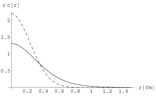
(a) Charm Wave Function

(b) Bottom Wave Function

Figure 3: (a) Calculated normalized wave function for the ground state $\Lambda_{c}$ from the complete potential (solid curve) and the harmonic approximation (dashed curve). (b) Calculated normalized wave function for the ground state $\Lambda_{b}$ from the complete potential (solid curve) and the harmonic approximation (dashed curve).

It is clear that for this particular model, both the shape of the wave function and the binding energy are vastly different when the entire effective potential is considered as compared to when the potential is assumed to be harmonic with the collective degree of freedom tightly localized. Large amplitude motion clearly occurs and the standard analysis appears to be invalid for this system.

For this system, orbital excited states can also be seen. Both the charm and bottom cases have an $l=1$ excited state; the binding energy is 42.0 MeV (charm) and 68.0 MeV (bottom). Neither system appears to have a bound $l=2$ state.

For the case when the light quark system carries spin 1, no bound states were found. The potential in this channel has a strong repulsive core with a very shallow attractive region which appears to be too weak to support bound states.

The previous calculations were performed using the assumption (valid in the heavy quark limit) that vector and pseudoscalar heavy mesons are degenerate. This is obviously not true in the physical case, that is, the $D$ and the $D^{*}$ or the $B$ and the $B^{*}$ have different masses. The calculation can be extended to include the physical mass splittings between the heavy meson states. When these splittings are included, there are still bound $\Lambda_{H}$ states, however, the binding is weaker. The binding energy of the ground state is reduced by 88.7 MeV for charm and 35.9 MeV for bottom.

To reiterate, these results clearly illustrate that the effective potential is not strong enough to localize the collective variable in the harmonic region for these models. The underlying assumption that the system is sufficiently close to the large $N_{c}$ and heavy quark limits to use the harmonic approximation is not justified. Clearly it is important to see whether the breakdown of the combined heavy quark and large $N_{c}$ limit is generic for realistic nucleon and heavy quark masses. This is particularly true since the model considered has serious phenomenological flaws, as will be discussed below. The key question is whether the standard treatment works for “realistic” models.

IV Towards the effective potential in realistic models

The model considered in the previous section is unsatisfactory in terms of phenomenology. In the first place the mass of the heavy baryons is well off from the empirical ones. The relevant issue is not how large the fractional error is for the mass since a large fraction of the mass is simply from the heavy quark itself. The relevant issue is the fractional error in the binding energy—i.e., the difference between the mass of a nucleon plus a heavy meson from the mass of the heavy baryon mass. In the model considered above $M_{n}+M_{D}-M_{\Lambda_{c}}$ = 155 MeV. In nature it is approximately 520 MeV. This is certainly not very good.

Moreover, the model considered above has the feature that the interaction is identical under the exchange of a heavy meson to a heavy anti-meson. That is, our extended potential will give the same bound states for ordinary heavy baryons as for heavy pentaquark states. Clearly this is unphysical. While heavy pentaquark states are known to exist in the extreme heavy quark and large $N_{c}$ limitshohler1 , there exists no symmetry of QCD in that limit which implies a degeneracy between pentaquarks and ordinary heavy baryons. Moreover, strong-interaction-stable heavy pentaquarks have not been detected despite intensive searches, suggesting that for realistic masses they do not exist.

If we wish to make a more realistic model it is necessary to include additional interaction terms between the heavy meson and the soliton which split the ordinary heavy baryon from the pentaquark. Such an interaction should be strong enough to give heavy baryons with approximately the correct mass. Heretofore, we have only included an interaction term between the pion fields and the heavy quark which was lowest order in the chiral expansion. However, in the soliton there is no chiral power counting and thus no necessity to restrict the interaction to this term. The spirit of model building in Skyrme type models is to include a small number of terms to make the problem tractable. Although there is no systematic power counting, the hope is that one can get qualitatively sensible results by choosing coefficients for these which compromise between the various observables. The simplest model realistic enough to get the binding of the heavy baryons correct while pushing up the mass of the heavy pentaquarks above threshold will require one new interaction term.

The simplest term that we can consider, which distinguishes between interactions between heavy mesons and anti-mesons, is coupling the light quark baryon current to the heavy quark vector current. Note that if a heavy anti-meson binds with a nucleon, the heavy quark current will switch sign compared with the heavy meson case while the baryon current (associated with the nucleon) will not. Therefore we add the term

$$\mathcal{L}_{\text{baryon}}=g^{\prime}\text{Tr}\bar{H}_{a}H_{a}\gamma_{\mu}B^{\mu}$$ (26)

to the Lagrangian, with the baryon current, $B^{\mu}$, given by the standard form,

$$B^{\mu}=\frac{\epsilon^{\mu\nu\alpha\beta}}{24\pi^{2}}\text{Tr}[(\Sigma^{\dagger}\partial_{\nu}\Sigma)(\Sigma^{\dagger}\partial_{\alpha}\Sigma)(\Sigma^{\dagger}\partial_{\beta}\Sigma)],$$ (27)

where the notation $\epsilon_{0123}=-\epsilon^{0123}=1$ was used. By inserting the functional form for the solitons into this term, and working in the rest frame of the heavy (anti)meson, the interacting potential can be derived as :

$$V_{\text{baryon}}(\vec{r})=g^{\prime}B^{0}(r)=\frac{g^{\prime}}{2\pi^{2}}\frac{\sin^{2}(F)}{r^{2}}F^{\prime}(r).$$ (28)

The coupling constant, $g^{\prime}$, and its relative sign are unknown, but the sign will be chosen such that this potential is attractive for heavy meson-nucleon interactions while repulsive for heavy anti-meson-nucleon interactions. In the spirit of this class of model, we will tune $g^{\prime}$ in order to get a reasonable mass for the heavy baryon (either $\Lambda_{b}$ or $\Lambda_{c}$). Of course, this procedure is quite ad hoc, but Skyrme type models always require some ad hoc procedure. One useful check on whether the model obtained is sensible is whether the the coupling obtained has a natural size, i.e., whether it is of $O(1)$.

When the Schödinger equation with the combined potential was used to calculate bound states, the coupling constants needed to have bound states with physical binding energies were determined to be -3.27 for $\Lambda_{c}$ and -3.34 for $\Lambda_{b}$. These are natural in size. Furthermore, the two coupling constants obtained via fitting for the two types of heavy baryons are quite close to one another; they differ by only 2% suggesting that the procedure is robust for physical values. For simplicity, the heavy meson mass splittings were not included in this calculation.

Because of the lack of the heavy meson mass splitting, we would expect that the first excited state to be a superposition of the two physically observed excited states, $\Lambda_{c}^{+}(2593)$ and $\Lambda_{c}^{+}(2625)$. It is not unbelievable to surmise that this combined state would weight the two states by the relative spins of the states. This would lead to a mass of the combined state of 2614 MeV or an excitation energy of 328 MeV above the ground state. With the coupling constants considered here, the excitation energy from the combined potential was found to be 324 MeV and 316 MeV for the charm and bottom cases, respectively. This is in surprisingly good agreement with the expected excitation from the physically seen states.

With the inclusion of the baryon current term to the potential, the light quark spin-1 state becomes bound for the coupling constants considered here. The binding energies are weak,; 125 MeV for charm and 173 MeV for bottom, compared with their spin-0 counterparts, $521.6$ MeV and 593.4 MeV for the $\Lambda_{c}$ and $\Lambda_{b}$, respectively. This binding is driven solely by the size of the baryon current coupling. The presence of a bound state in the spin-1 channel does not invalidate nor should it limit our method. It is not unreasonable to believe that the strength of the additional potentials that is needed to be included to drive the binding energy down to physical values might also bind light quark spin-1 states. Therefore the lack of any observation of these states could be associated with the difficulty in detection and not in the lack of the presence of these states.

A harmonic approximation can also be made for the combined potential with the provided coupling constants. The energy levels for the approximation are again different from that of the combined potential and the ground state is bound weaker. An examination of the shape of the wave function for the combined potential compared with the harmonic wave functions shows again that the wave functions for the combined potential are broader than the harmonic wave functions and extend beyond the harmonic region. We again find ourselves not driven to the effective potential minimum by the realistic masses suggesting that the physical states are not close to the extreme large $N_{c}$ and heavy quark limits. These observations confirm the results from the previous section that the long distance potential greatly influences heavy baryon formation.

Unlike with our original potential, the new combined potential is sensitive to the difference between regular heavy baryons and heavy pentaquarks. We can examine whether a bound pentaquark state is possible within the combined potential by flipping the sign of the coupling constant of the baryon current term. When this is performed, a very weakly bound pentaquark state can be found with a binding energy of $33.4$ MeV for a charm type pentaquark, and $42.9$ MeV for a bottom type pentaquark. These are rather small binding energies compared with the binding energies of the regular heavy baryons, and are small compared to the deeply bound pentaquark states suggested by the large $N_{c}$ and heavy quark limits hohler1 . Furthermore, the potential for the heavy pentaquark is repulsive at short distance creating the attractive region and localization of the wave function away from the origin. Therefore, even in the ground state, the pentaquark formed here has a fixed separation between the heavy anti-meson and the nucleon. However, due to the strong repulsion at short distance this is a very delicate state. If we turn off the potential which is identical for the heavy baryon and heavy pentaquark states, and tune the baryon current coupling such that heavy baryons are still bound with the appropriate binding energy, we find that the heavy pentaquark effective potential is completely repulsive and thereby no heavy pentaquark state is bound. The coupling constants needed to achieve this condition were -5.52 for the charm case and -5.49 for the bottom case. These couplings are again neither unreasonably large nor small. This indicates that this model is capable of binding a heavy pentaquark state, but with minor changes it is just as reasonable not to support a bound heavy pentaquark state. The relative ease for the state to become unbound furthers the point in hohler1 that heavy pentaquark binding with physically reasonable parameters is subject to the dynamical details of the model.

We have justified the inclusion of an additional interaction term based upon the coupling of the heavy quark current to the baryon current. This interaction was derived for all separation distances. The coupling of the interaction was determined by having the ground state binding energy correspond to the physical value. With this potential in place, our simple model gives phenomenologically reasonable results concerning ordinary heavy baryons while simultaneously being reasonably consistent and inconsistent with a bound heavy pentaquark state.

V Calculation of the Isgur-Wise Function

The Isgur-Wise function is a universal function in the heavy quark limit that describes the semileptonic decay of all heavy hadrons in an SU(2$N_{H}$) multiplet (where $N_{H}$ is the number of heavy flavors). In our case we can consider heavy hadrons of the $\Lambda$ type isgurwise . Thus the process in question is $\Lambda_{b}\rightarrow\Lambda_{c}e^{-}\bar{\nu}_{e}$ Ṗrevious work has shown that the Isgur-Wise function is completely determined in the combined large $N_{c}$ and heavy quark limit jm . In this limit the effective potential is purely harmonic in nature, and the Isgur-Wise function would be dependent on only one parameter, the harmonic “spring constant” ck1 ; ck2 . Therefore it has been pointed out that if the excitation energy of heavy baryons were measured, the spring constant would be fixed and thus Isgur-Wise function would be completely determined up to higher order corrections.

Unfortunately, we have shown thus far that for realistic parameters, the system does not remain in the harmonic region and the expansion appears to break down. Of course, from the wave functions we have already calculated, the Isgur-Wise function can also be calculated, and again we would expect distinct results from the harmonic oscillator case.

The most interesting aspect of the Isgur-Wise function near the combined limit is related to the fact that this entire universal function is dependent on one measurable parameter. We wish to test the reliability of this result when one deviates from the ideal limit, viz., for the real world. Ideally one could test this by using the empirical value of the excitation energy of the first excited state plus the assumption that one is near the combined large $N_{c}$ and heavy quark limits to compute the Isgur-Wise function; this ought then to be compared with the experimental Isgur-Wise function for an empirical test. However, the Isgur-Wise form factors have not been measured.

In the absence of such data, we can still get some idea of how robust is the prediction by using “realistic” models. Since these models indicate that that system is quite anharmonic, we do not expect a close agreement of the Isgur-Wise function with the harmonic approximation based on the energy of the first excited state. Instead of considering the entire Isgur-Wise function, we will focus our attention on the curvature at zero recoil, $\rho$, of the Isgur-Wise function. We chose to do this as $\rho$ is proportional to the mean radius squared in the heavy quark limit, and thereby provides a single number with which to compare and does so in a physically transparent way.

The Isgur-Wise function in momentum space from jm is

$$\eta_{0}=\int\!\!d^{3}\vec{p}\;\phi^{*}_{c}(\vec{p}+m_{N}\vec{v}^{\prime})\,\phi_{b}(\vec{p}).$$ (29)

In the case of harmonic wave functions this reduces to

$$\eta_{HO}(z)=\frac{2\sqrt{2}\mu_{b}^{3/8}\mu_{c}^{3/8}}{(\sqrt{\mu_{b}}+\sqrt{\mu_{c}})^{3/2}}\,\text{Exp}\Bigl{[}\frac{-z^{2}}{2\sqrt{\kappa}}\Bigr{]},\quad\text{where}\quad z\equiv\frac{m_{N}|\vec{v}|}{(\sqrt{\mu_{b}}+\sqrt{\mu_{c}})^{1/2}},$$ (30)

$m_{N}$ is the mass of the nucleon, $\kappa$ is the harmonic coupling, $\vec{v}$ is the transfer velocity, and $\mu_{c}$ and $\mu_{b}$ are the reduced mass of the heavy meson-nucleon system for either charm or bottom, respectively. We can also express the Isgur-Wise function in terms of position space wave function as

$$\eta_{0}=\int\!\!d^{3}\vec{x}\;\psi_{c}^{*}(\vec{x})\psi_{b}(\vec{x})\,\frac{\sin(\frac{m_{N}}{|\vec{v}||\vec{x}|})}{m_{N}|\vec{x}||\vec{v}|}.$$ (31)

These expressions for the Isgur-Wise function lead to the following leading order expressions for the curvature at zero recoil,

$$\rho_{HO}\equiv\frac{\partial^{2}\eta_{HO}}{\partial z^{2}}(z=0)=-\frac{2\sqrt{2}\mu_{b}^{3/8}\mu_{c}^{3/8}}{\sqrt{\kappa}\,(\sqrt{\mu_{b}}+\sqrt{\mu_{c}})^{3/2}}$$ (32)

for the harmonic case, and

$$\rho\equiv\frac{\partial^{2}\eta}{\partial z^{2}}(z=0)=-\frac{\sqrt{\mu_{b}}+\sqrt{\mu_{c}}}{3}\int\!\!d^{3}\vec{x}\;\psi^{*}_{c}(\vec{x})\psi_{b}(\vec{x})|\vec{x}|^{2}$$ (33)

for the spatial wave function case.

We will calculate $\rho$ in three different manners. First, $\rho$ can be calculated by approximating the potential by a harmonic oscillator to generate a harmonic coupling, $\kappa$. Equation (32) can then be used for this value of $\kappa$, along with physical values of the mass variables, to calculate $\rho$. Second, the wave functions of the ground state of the complete potential can be used directly in Eq. (33) to calculate $\rho$. Of course, this is the proper way to calculate $\rho$ and the Isgur-Wise function since the complete potential is being considered. We would expect a vast difference between the first two methods since we have been observing differences in the wave function between the harmonic wave functions and the complete potential wave functions. Lastly, even though we know that the energy levels calculated by using the entire effective potential are not harmonic in nature, we could use the excitation energy of the first excited state to calculate $\kappa$ as though it were derived from a harmonic oscillator, and then use this value of $\kappa$ to calculate $\rho$ using Eq. (32). That is, instead of deriving the harmonic coupling from an approximation to the actual potential, we are constructing a new harmonic potential, which is unrelated to the original harmonic potential and to the complete potential, except that the energy gap between the ground state and the first excited state of this new potential and the complete potential are identical. Of course, the third method has no underlying theoretical basis unless the system is harmonic (in which case it will agree with the first two). It is useful to consider it, however, because it simulates theoretically the empirical procedure outlined above.

When the curvature of the Isgur-Wise function at zero recoil, $\rho$, was calculated in these manners, using physical mass of the nucleon and the heavy baryons, the following results were obtained. The normalized wave functions are shown in Fig. 4, remembering that $\rho$ is proportional to the expectation value of $r^{2}$.

(a) Charm Wave Functions

(b) Bottom Wave Function

Figure 4: (a) Calculated normalized wave functions for the ground state $\Lambda_{c}$ from the complete potential (solid curve), the harmonic approximation (smaller dashed curve), and the harmonic approximation from the excitation energy (larger dashed curve). (b) Calculated normalized wave functions for the ground state $\Lambda_{b}$ form the complete potential (solid curve), the harmonic approximation (smaller dashed curve), and the harmonic approximation from the excitation energy (larger dashed curve).

Method 1 yielded $-53.8\times 10^{-6}\text{MeV}^{-3/2}$ when $g^{\prime}$ was chosen to have the appropriate coupling constant for the bottom sector. Method 2 yields $-121\times 10^{-6}\text{MeV}^{-3/2}$. Note that by using the complete wave functions, the curvature is a factor of 2 larger than the case of using harmonic oscillator wave functions. Lastly, Method 3, of using the excitation energy from the full potential and assuming it came from a harmonic oscillator potential, yields $-111\times 10^{-6}\text{MeV}^{-3/2}$ with the bottom case coupling constant. This result is different from the Method 1 as one might have expected, but is quite similar to the Method 2 (which gives the “correct” result). This is quite surprising since Method 3 can only be justified via the harmonic approximation which appears to be badly violated (as seen from the result of Method 1). Given the fact that Method 3 simulates the natural way to test the harmonic approximation empirically, it is important to test whether the success of Method 3 in getting close to the correct result is a mere numerical accident for this model or whether it is a robust feature. As we will see it is quite robust.

In order to test the extent to whether Method 3 generically reproduces the correct result of Method 2, one needs to consider a wide variety of models and compare the results. Since the effective potential only depends on the Skyrme profile function we have considered a variety of profile functions (which we constructed on an ad hoc basis entirely for the purpose of testing the validity of Method 3). The curvature at zero recoil of the Isgur-Wise function was calculated for these effective potentials using the three methods detailed above. The effective potentials that were considered are shown in Fig. 5 while the results of the calculations of $\rho$ are presented in Table 1. One can clearly see that with all effective potentials considered, the curvature at zero recoil calculated with harmonic wave functions is different from the calculations performed with the other two methods. However, for all the potentials considered, the latter two methods provide similar results. Although not depicted in Table 1, when an effective potential with a global minimum away from the origin is considered, Methods 2 and 3 give different results. This can be attributed to the wave function calculated with the complete effective potential being peaked away from the origin, where Method 3 assumes that the wave function is still peaked at the origin.

Figure 5: Variety of effective potentials: (a) solid curve; (b) long dashed curve; (c) short dashed curve; (d) dotted curve; (e) dot-dashed curved.

Potential	Method 1	Method 2	Method 3
a (Original)	-53.8	-121	-111
b	-83.3	-175	-171
c	-109	-216	-215
d	-101	-142	-139
e	-132	-225	-231

Table 1: The curvature at zero recoil, $\rho$, of the Isgur-Wise function calculated in three different manners in units of $10^{-6}\text{MeV}^{-3/2}$. The first line is the original profile function we considered. All calculations were performed with the coupling constant, $g^{\prime}$, chosen to bind $\Lambda_{b}$ with the appropriate binding energy.

The fact that Method 3 works so well, even when the system is quite anharmonic, appears to have some important consequences. In the first place, it means the prediction of $\rho$ from the excited state energy (using the harmonic approximation) may be expected to hold reasonably well and, hence, one has some real predictive power even if the system is rather anharmonic. The converse of this appears to be that the degree to which $\rho$ is accurately predicted via Method 3 is a poor test of the degree to which the system is harmonic.

In fact, the situation is a bit more subtle than this. Qualitatively it is clear what is happening: the anharmonic nature of the potential lowers the excitation energy compared to that of a harmonic potential with the same curvature at the minimum. Fitting this excitation with a harmonic oscillator means that the fitted oscillator will have a smaller curvature (i.e., spring constant) than the actual spring constant at the minimum. This has the effect of spreading out the wave function compared to the harmonic approximation based on the true curvature which in turn means a larger value of $\rho$; this acts to simulate the true wave function which is also wider than the naive harmonic result. Thus, generically, the sign of the effect of anharmonicity on the excitation energy and $\rho$ helps explain the viability of Method 3. The degree to which the method works quantitatively may still seem remarkable, however. The quantitative success is at least partially understandable analytically. It is straightforward to calculate the leading order effect of the anharmonicity on both the excitation energy of the lowest excited state ck2 . As it happens, the shift in the excitation energy exactly compensates the shift in $\rho$ to leading order in the anharmonicity, and the according inaccuracies due to using Method 3 only appear at next-to-next-to leading order. Thus, the system can be rather anharmonic and Method 3 can remain reasonably accurate. It is nevertheless remarkable how well Method 3 appears to work since the wave functions appear to be qualitatively quite different from the harmonic ones of Method 1.

In conclusion, we have constructed the effective potential for the binding of the heavy (anti-)meson and nucleon to form regular and exotic heavy baryons for variations of the Skyrme model. We have demonstrated that this effective potential gives excitation energies and collective wave functions which are qualitatively different from those obtained with a harmonic oscillator approximation to the potential: the wave functions with realistic particle masses are not concentrated near the potential minimum, as expected from the large $N_{c}$ and heavy quark limits. This indicates that the masses are not heavy enough to have heavy baryons exhibit the properties of these limits. Calculations with the full effective potential showed that heavy pentaquark states are possible in this class of model but the existence of bound pentaquarks depends sensitively on the details of the model studies. We also showed that despite strong anharmonicities the description of the Isgur-Wise function derived from the harmonic approximation works remarkably well provided that the effective harmonic coupling derived from the first excitation energy is used.

Acknowledgments. T.D.C. and P.M.H. were supported by the D.O.E. through grant DE-FGO2-93ER-40762.

References

- (1) Z. Guralnik, M. Luke, and A.V. Manohar, Nucl. Phys. B 390, 474 (1993).
- (2) E. Jenkins, A.V. Manohar, and M.B. Wise, Nucl. Phys. B 396, 27 (1993).
- (3) E. Jenkins, A.V. Manohar, and M.B. Wise, Nucl. Phys. B 396, 38 (1993).
- (4) Z.A. Baccouche, C-K Chow, T.D. Cohen, and B.A. Gelman, Nucl. Phys. A 696, 638 (2001).
- (5) Z.A. Baccouche, C-K Chow, T.D. Cohen, and B.A. Gelman, Phys. Lett. B 514, 346 (2001).
- (6) C-K. Chow, T.D. Cohen, and B.A. Gelman, Nucl. Phys. A 692, 521 (2001); B.A. Gelman hep-ph/0203246.
- (7) T.H.R. Skyrme, Proc. Roy. Soc. A 260, 127 (1961).
- (8) E. Witten, Nucl. Phys. B 223, 433 (1983).
- (9) J. Wess and B. Zumino, Phys. Lett. B 37, 95 (1971).
- (10) G.S. Adkins, C.R. Nappi, and E. Witten, Nucl. Phys. B 228, 552 (1983).
- (11) E. Guadagnini, Nucl. Phys. B 236, 35 (1984).
- (12) A.V. Manohar, Nucl. Phys. B 248, 19 (1984).
- (13) C.G. Callan and I. Klebanov, Nucl. Phys. B 262, 365 (1985).
- (14) C.G. Callan, K. Hornbostel, and I. Klebanov, Phys. Lett. B 202, 269 (1988)
- (15) M.B. Wise, Phys. Rev. D 45, R2188 (1992).
- (16) G. Burdman and J.F. Donoghue, Phys. Lett. 280B, 287 (1992).
- (17) T-M Yan, H-Y Cheng, C-Y Cheung, G-L Lin, Y.C. Lin, and H-L Yu, CLNS 92/1138 (1992).
- (18) N. Itzhaki, I.R. Klebanov, P. Ouyang, and L. Rastelli, Nucl. Phys. B 684, 264 (2004).
- (19) T.D. Cohen, P.M. Hohler, and R.F. Lebed, Phys. Rev. D 72, 074010 (2005).
- (20) N. Isgur and M.B. Wise, Phys. Lett. B 232, 113 (1989), Phys. Lett. B 237, 527 (1990).
- (21) Y. Oh and B.-Y. Park, Z. Phys. A 359, 83 (1997); Y. Oh and B.-Y. Park, Mod. Phys. Lett. A 11, 653 (1996); Y. Oh and B.-Y. Park, Phys. Rev. D 53, 1605 (1996); Y. Oh and B.-Y. Park, Phys. Rev. D 51, 5016 (1995); D.-P. Min, Y. Oh, B.-Y. Park, and M. Rho, Int. Jour. Mod. Phys. E 4, 47 (1995); Y. Oh, B.-Y. Park, and D.-P. Min, Phys. Rev. D 50, 3350 (1994); Y. Oh , B.-Y. Park, and D.-P. Min, Phys. Lett. B 331, 362 (1994)
- (22) I.W. Stewart, M.E. Wessling, M.B. Wise, Phys. Lett. B 590, 185 (2004).
- (23) M.E. Wessling, Phys. Lett. B 603, 152 (2004); 618, 269 (2005); Ph.D. Thesis, Caltech, hep-ph/0505213.
- (24) C. Gignoux, B. Silvestre-Brac, and J.M. Richard, Phys. Lett. B 193, 323 (1987); H. Lipkin, Phys. Lett. B 195, 484 (1987); F. Stancu, Phys. Rev. D 58, 111501(R) (1998); M. Genovese, J.M. Richard, F. Stancu, and S. Pepin, Phys. Lett. B 425, 171 (1998).
- (25) D. Diakonov, V. Petrov, and M.V. Polyakov, Z. Phys. A 359 305 (1997).
- (26) H. Walliser and H. Weigel, Eur. Phys. J. A 26, 361 (2005); hep-ph/0511297.
- (27) T.D. Cohen, Phys. Lett. B 581, 175 (2004); T.D. Cohen and R.F. Lebed, Phys. Lett. B 578, 150 (2004); T.D. Cohen, Phys. Rev. D 70, 014011 (2004); T.D. Cohen, hep-ph/0511174.
- (28) A. Cherman, T.D. Cohen, A. Nellore, Phys. Rev. D 70, 096003 (2004); A. Cherman, T.D. Cohen, T.R. Dulaney, E.M. Lynch, Phys. Rev. D 72, 094015 (2005).
- (29) G. Duplancic and J. Trampetic, Phys. Rev. D 69, 117501 (2004).
- (30) R.L. Jaffe and F. Wilczek, Phys. Rev. Lett. 91, 232003 (2003); Phys. Rev. D 69, 114017 (2004).
- (31) V.B. Kopeliovich, Phys. Part. Nucl. 37, 623 (2006), Fiz. Elem. Chast. Atom. Yadra. 37, 1184 (2006).
- (32) M. Karliner, H.J. Lipkin, hep-ph/0307343; Phys. Lett. B 575, 249 (2003).
- (33) T.D. Cohen, Phys. Rev. D 70, 074023 (2004)
- (34) A.P. Balachandran, A. Barducci, F. Lizzi, V.G.J. Rodgers, A. Stern, Phys. Rev. Lett. 52, 887 (1984); A.P. Balachandran, F. Lizzi, V.G.J. Rodgers, A. Stern, Nucl. Phys. B 256, 525 (1985).
- (35) G. Duplancic, H. Pasagic, M. Praszlowicz, J. Trampetic, Phys. Rev. D 64, 097502 (2001).
- (36) C.K. Chow and T.D. Cohen, Phys. Rev. Lett. 84, 5474 (2000), C.K. Chow and T.D. Cohen, Nucl. Phys. A 688, 842 (2001).
- (37) N. Isgur and M.B. Wise, Adv. Ser. Direct. High Energy Phys. 10, 549 (1992).
- (38) G.S. Adkins and C.R. Nappi, Nucl. Phys. B 233, 109 (1984).
- (39) A.V. Manohar and M.B. Wise, Camb. Monogr. Part. Phys. Nucl. Phys. Cosmol. 10, 1-191 (2000).
- (40) A. Anastassov et al. (CLEO Collaboration), Phys. Rev. D 65, 032003 (2002).
- (41) W.-M. Yao et al. (Particle Data Group), J. Phys. G 33, 1 (2006).