The azimuthal decorrelation of jets widely separated in rapidity as a test of the BFKL kernel

Abstract

We study the decorrelation in azimuthal angle of Mueller–Navelet jets at hadron colliders within the BFKL formalism. We introduce NLO terms in the evolution kernel and present a collinearly–improved version of it for all conformal spins. We show how this further resummation has good convergence properties and is closer to the Tevatron data than a simple LO treatment. However, we are still far from a good fit. We offer estimates of these decorrelations for larger rapidity differences which should favor the onset of BFKL effects and encourage experimental studies of this observable at the LHC.

CERN–PH–TH/2007–029
DESY–07–017

1 Introduction

In this paper we continue the analytic study of the azimuthal decorrelations in Mueller–Navelet jets using the Balistky–Fadin–Kuraev–Lipatov (BFKL) equation [1] beyond the leading order approximation initiated in Ref. [2]. We investigate the inclusive hadroproduction of a pair of jets with large and similar transverse momenta produced at a large relative rapidity separation Y [3]. In principle, when this rapidity Y between the most forward and most backward jets is small there is not much phase space for the production of extra radiation and a fixed order perturbative calculation should be enough to describe the observable. However, if Y is large enough to make the product ${\alpha}_{s}Y\sim 1$ then a BFKL resummation of these terms to all orders should improve the accuracy of the calculation.

In Section 2 we define our observables at partonic level and argue that the particular choice of rapidity variable removes the dependence on the parton distribution functions in normalized cross sections. The explicit expressions for angular differential cross sections including the next–to–leading (NLO) BFKL kernel [4] with full angular dependence are also presented. In Section 3 we study in detail the structure of the scale invariant NLO BFKL kernel for different conformal spins. We show how the convergence of this kernel in terms of asymptotic intercepts is poor for zero conformal spin while being much better for larger ones. After this, a prescription to improve the collinear structure of the kernel using a shifted anomalous dimension for the full angular dependence is derived. The main consequence of this study is that even though collinear poles are removed for all conformal spins only the asymptotic intercept corresponding to the angular averaged case is modified, while the intercepts of the angular dependent components are hardly affected by the resummation. In Section 4 we use these kernels to make predictions for hadron colliders. We further discuss the need of a collinear resummation to generate stable results against a change of renormalization scheme and show that the resummed results provide a better description of the Tevatron data than those using LO BFKL. However, our results provide too much decorrelation when they are compared to the experimental measurements. From the theoretical side this could be due to the approximations needed to obtain our analytic results, e.g., the choice of rapidity variable and use of leading order jet vertices. In principle, our predictions should be more reliable at larger rapidities where multiple emissions between the two tagged jets are favored. It would be very interesting to further study these Mueller–Navelet jets at the Large Hadron Collider (LHC) at CERN to gauge the importance of configurations in multi–Regge and quasi–multi–Regge kinematics and try to investigate other possible jet topologies dominated by them. This point is further discussed at the end of our work, in the Conclusions section.

2 Cross sections

We are interested in the study of normalized differential cross sections which turn out to be quite insensitive to the parton distribution functions. Therefore, to a good accuracy, the present analysis can be performed at partonic level and we focus on the ${\rm parton}+{\rm parton}\rightarrow{\rm jet}+{\rm jet}+{\rm soft}\,\,{\rm emission}$ process. The differential cross section is then

$$\frac{d{\hat{\sigma}}}{d^{2}\vec{q}_{1}d^{2}\vec{q}_{2}} = \frac{\pi^{2}{\bar{\alpha}}_{s}^{2}}{2}\frac{f\left(\vec{q}_{1},\vec{q}_{2},{\rm Y}\right)}{q_{1}^{2}q_{2}^{2}},$$ (1)

where ${\bar{\alpha}}_{s}=\alpha_{s}N_{c}/\pi$ is the strong coupling, $\vec{q}_{1,2}$ are the transverse momenta of the tagged jets, and Y their relative rapidity. The influence of the distribution functions is larger if the exact definition of the rapidity difference as in Fig. 1 is considered. For convenience we take Y as a fixed parameter since this allows us to perform all the necessary Mellin transforms and proceed with our analysis analytically. In more detail, the choice ${\rm Y}=\ln{(x_{1}x_{2}s/s_{0})}$ corresponds to a change of the energy scale $s_{0}=\sqrt{\vec{q}_{1}^{2}\vec{q}_{2}^{2}}$ to a fixed value. This change can be also understood as a NLO contribution to the vertices coupling the tagged jets to the external hadrons. The uncertainty associated to the choice of $s_{0}$ will be taken into account in the phenomenological discussion at the end of Section 4.

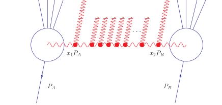
Figure 1: Representation of Mueller–Navelet jets at a hadron collider.

The gluon Green’s function

$$f\left(\vec{q}_{1},\vec{q}_{2},{\rm Y}\right) = \int\frac{d\omega}{2\pi i}e^{\omega{\rm Y}}f_{\omega}\left(\vec{q}_{1},\vec{q}_{2}\right),$$ (2)

carries the full dependence on Y and fulfills the NLO BFKL equation which, in the transverse momenta operator representation

$${\hat{q}}\left|\vec{q}_{i}\right> = \vec{q}_{i}\left|\vec{q}_{i}\right>,$$ (3)

with normalization

$$\left<\vec{q}_{1}\right|{\hat{1}}\left|\vec{q}_{2}\right> = \delta^{(2)}\left(\vec{q}_{1}-\vec{q}_{2}\right),$$ (4)

can be written as

$$\left(\omega-{\bar{\alpha}}_{s}{\hat{K}}_{0}-{\bar{\alpha}}_{s}^{2}{\hat{K}}_{1}\right){\hat{f}}_{\omega} = {\hat{1}}.$$ (5)

This representation is useful when it acts on the basis

$$\left<\vec{q}\right|\left.\nu,n\right> = \frac{1}{\pi\sqrt{2}}\left(q^{2}\right)^{i\nu-\frac{1}{2}}\,e^{in\theta},$$ (6)

which includes the dependence on the modulus and azimuthal angle of the different emissions. The Mellin–conjugate variable of the modulus is the real parameter $\nu$, and the Fourier–conjugate parameter of the angle is the integer conformal spin $n$.

As the rapidity difference increases the azimuthal angle dependence is mainly driven by the kernel. This is the reason why, in the present work, we make use of the LO jet vertices which are much simpler than the NLO ones calculated in Ref. [5]. Following Ref. [2] we can then write the differential cross section in the azimuthal angle $\phi=\theta_{1}-\theta_{2}-\pi$, where $\theta_{i}$ are the angles corresponding to the two tagged jets, as

$$\frac{d{\hat{\sigma}}\left(\alpha_{s},{\rm Y},p_{1,2}^{2}\right)}{d\phi} = \frac{\pi^{2}{\bar{\alpha}}_{s}^{2}}{4\sqrt{p_{1}^{2}p_{2}^{2}}}\sum_{n=-\infty}^{\infty}e^{in\phi}\,{\cal C}_{n}\left({\rm Y}\right),$$ (7)

with

$${\cal C}_{n}\left({\rm Y}\right) = \frac{1}{2\pi}\int_{-\infty}^{\infty}\frac{d\nu}{\left(\frac{1}{4}+\nu^{2}\right)}\left(\frac{p_{1}^{2}}{p_{2}^{2}}\right)^{i\nu}e^{\chi\left(\left|n\right|,\frac{1}{2}+i\nu,{\bar{\alpha}}_{s}\left(p_{1}p_{2}\right)\right){\rm Y}},$$ (8)

and

$$\chi\left(n,\gamma,{\bar{\alpha}}_{s}\right) \equiv {\bar{\alpha}}_{s}\chi_{0}\left(n,\gamma\right)+{\bar{\alpha}}_{s}^{2}\left(\chi_{1}\left(n,\gamma\right)-\frac{\beta_{0}}{8N_{c}}\frac{\chi_{0}\left(n,\gamma\right)}{\gamma\left(1-\gamma\right)}\right).$$ (9)

Throughout this work, the coefficients ${\cal C}_{n}$ are not evaluated at the saddle point, but obtained by a numerical integration over the full range of $\nu$. In the above expression the LO kernel, $\hat{K}_{0}$, has as eigenvalue the function

$$\chi_{0}\left(n,\gamma\right) = 2\psi\left(1\right)-\psi\left(\gamma+\frac{n}{2}\right)-\psi\left(1-\gamma+\frac{n}{2}\right),$$ (10)

with $\psi$ being the logarithmic derivative of the Euler gamma function. The last term in Eq. (9) stems from the scale dependent part of the NLO kernel, i.e. from the running of the coupling. Its explicit form, in our representation, depends on the impact factors and is discussed in more detail in Refs. [2, 7]. The action of the scale invariant sector of the NLO correction, $\hat{K}_{1}$, in the $\overline{\rm MS}$ renormalization scheme, on the basis in Eq. (6) explicitly reads [8]

$$\chi_{1}\left(n,\gamma\right) = {\cal S}\chi_{0}\left(n,\gamma\right)+\frac{3}{2}\zeta\left(3\right)-\frac{\beta_{0}}{8N_{c}}\chi_{0}^{2}\left(n,\gamma\right)$$ (11)

$$+ \frac{1}{4}\left[\psi^{\prime\prime}\left(\gamma+\frac{n}{2}\right)+\psi^{\prime\prime}\left(1-\gamma+\frac{n}{2}\right)-2\,\phi\left(n,\gamma\right)-2\,\phi\left(n,1-\gamma\right)\right]$$

$$- \frac{\pi^{2}\cos{\left(\pi\gamma\right)}}{4\sin^{2}\left(\pi\gamma\right)\left(1-2\gamma\right)}\left\{\left[3+\left(1+\frac{n_{f}}{N_{c}^{3}}\right)\frac{2+3\gamma\left(1-\gamma\right)}{\left(3-2\gamma\right)\left(1+2\gamma\right)}\right]\delta_{n}^{0}\right.$$

$$\left.\hskip 56.9055pt-\left(1+\frac{n_{f}}{N_{c}^{3}}\right)\frac{\gamma\left(1-\gamma\right)}{2\left(3-2\gamma\right)\left(1+2\gamma\right)}\delta_{n}^{2}\right\},$$

where we have used the notation ${\cal S}=\left(4-\pi^{2}+5\beta_{0}/N_{c}\right)/12$, $\beta_{0}=(11N_{c}-2n_{f})/3$ and $\zeta(n)=\sum_{p=1}^{\infty}p^{-n}$ is the Riemann zeta function. The $\phi(n,\gamma)$ function is of the form

$$\phi(n,\gamma) = \sum_{k=0}^{\infty}\frac{(-1)^{(k+1)}}{k+\gamma+\frac{n}{2}}\left(\frac{}{}\psi^{\prime}(k+n+1)-\psi^{\prime}(k+1)\right.$$ (12)

$$\left.+(-1)^{(k+1)}\left(\beta^{\prime}(k+n+1)+\beta^{\prime}(k+1)\right)+\frac{\psi(k+1)-\psi(k+n+1)}{k+\gamma+\frac{n}{2}}\right),$$

with

$$4\,\beta^{\prime}(\gamma) = \psi^{\prime}\left(\frac{1+\gamma}{2}\right)-\psi^{\prime}\left(\frac{\gamma}{2}\right).$$ (13)

These scale invariant eigenvalues have a very interesting structure which we will study in the next section. Before this we would like to indicate that the full cross section corresponds to the integration over the azimuthal angle of the differential expression in Eq. (7). This implies that it only depends on the $n=0$ component:

$${\hat{\sigma}}\left(\alpha_{s},{\rm Y},p_{1,2}^{2}\right) = \frac{\pi^{3}{\bar{\alpha}}_{s}^{2}}{2\sqrt{p_{1}^{2}p_{2}^{2}}}\,{\cal C}_{0}\left({\rm Y}\right).$$ (14)

In this paper we are interested in those distributions which are sensitive to the higher conformal spins. In particular, the average of the cosine of the azimuthal angle times an integer projects out the contribution from each of these angular components. It can be obtained using the ratio

$$\left<\cos{\left(m\phi\right)}\right> = \frac{{\cal C}_{m}\left({\rm Y}\right)}{{\cal C}_{0}\left({\rm Y}\right)}.$$ (15)

The associated ratios

$$\frac{\left<\cos{\left(m\phi\right)}\right>}{\left<\cos{\left(n\phi\right)}\right>} = \frac{{\cal C}_{m}\left({\rm Y}\right)}{{\cal C}_{n}\left({\rm Y}\right)}$$ (16)

are also of interest since they can be used to remove the uncertainty associated to the hard pomeron intercept, i.e. the $n=0$ component, which we will analyze below. To study the behavior of all the angular components together it is useful to use the normalized differential cross section on the azimuthal angle:

$$\frac{1}{{\hat{\sigma}}}\frac{d{\hat{\sigma}}}{d\phi}~{}=~{}\frac{1}{2\pi}\sum_{n=-\infty}^{\infty}e^{in\phi}\frac{{\cal C}_{n}\left({\rm Y}\right)}{{\cal C}_{0}\left({\rm Y}\right)}~{}=~{}\frac{1}{2\pi}\left\{1+2\sum_{n=1}^{\infty}\cos{\left(n\phi\right)}\left<\cos{\left(n\phi\right)}\right>\right\}.$$ (17)

Before comparing the results stemming from these expressions with the experimental data it is important to first analyze the convergence of the kernel at NLO for the different conformal spins. We proceed with this study in the coming section.

3 Collinear resummation

It is well–known that the BFKL resummation presents an instability when the NLO corrections are taken into account, for details regarding this point, see, e.g., Refs. [6, 9, 10]. For the observables studied in this paper we have found that if we use the NLO BFKL kernel as it stands the cross sections are very dependent on the renormalization scheme. In particular, the term proportional to $\chi_{0}$ in $\chi_{1}$ can be removed by a shift of the Landau pole of the form

$$\Lambda_{\overline{\rm MS}}\rightarrow\Lambda_{\rm GB}=\Lambda_{\overline{\rm MS}}e^{\frac{2N_{c}}{\beta_{0}}{\cal S}}.$$ (18)

This defines the so–called gluon–bremsstrahlung (GB) scheme [11, 12] which is commonly used when dealing with soft gluon resummations. In this new scheme we find that some of our distributions even change sign and become unphysical. This is a manifestation of the poor convergence of the series. A crucial ingredient to improve the convergence of the perturbative expansion is to demand compatibility of the BFKL kernel with renormalization group evolution to all orders in the limit of deep inelastic scattering. This can be achieved if corrections to all orders are introduced by means of a shift in the anomalous dimension [13]. So far these types of resummations have been performed for a BFKL kernel averaged over the azimuthal angle and therefore they only affect the zero conformal spin sector. For our purposes in this work we must study the convergence of the eigenvalues of the kernel for all angular components.

The renormalization group improved kernels are based on a proper treatment of the collinear region of emissions. This region is insensitive to the azimuthal angle so we should not find a big effect beyond the $n=0$ case when we resum. We will see that this is the case because the asymptotic intercepts for the different angular components with $n>0$ are very stable under radiative corrections.

To start our investigation it is necessary to extract the pole structure of the different contributions to the kernel around the $\gamma=-\frac{n}{2},1+\frac{n}{2}$ points. These poles are as follows:

$$\chi_{0}\left(n,\gamma\right) \simeq \frac{1}{\gamma+\frac{n}{2}}+\left\{\gamma\rightarrow 1-\gamma\right\},$$ (19)

$$\chi_{1}\left(n,\gamma\right) \simeq \frac{a_{n}}{\gamma+\frac{n}{2}}+\frac{b_{n}}{\left(\gamma+\frac{n}{2}\right)^{2}}-\frac{1}{2\left(\gamma+\frac{n}{2}\right)^{3}}+\frac{c\,\delta_{n}^{2}}{\gamma}+\left\{\gamma\rightarrow 1-\gamma\right\}.$$ (20)

The coefficients at the singular points can be written as

$$a_{n} = {\cal S}-\frac{\pi^{2}}{24}+\frac{\beta_{0}}{4N_{c}}{\rm H}_{n}+\frac{1}{8}\left(\psi^{\prime}\left(\frac{n+1}{2}\right)-\psi^{\prime}\left(\frac{n+2}{2}\right)\right)+\frac{1}{2}\psi^{\prime}\left(n+1\right)$$ (21)

$$- \frac{\delta_{n}^{0}}{36}\left(67+13\frac{n_{f}}{N_{c}^{3}}\right)-\frac{47\delta_{n}^{2}}{1800}\left(1+\frac{n_{f}}{N_{c}^{3}}\right),$$

$$-b_{n} = \frac{\beta_{0}}{8N_{c}}+\frac{1}{2}{\rm H}_{n}+\frac{\delta_{n}^{0}}{12}\left(11+2\frac{n_{f}}{N_{c}^{3}}\right)+\frac{\delta_{n}^{2}}{60}\left(1+\frac{n_{f}}{N_{c}^{3}}\right),$$ (22)

$$c = \frac{1}{24}\left(1+\frac{n_{f}}{N_{c}^{3}}\right).$$ (23)

Here ${\rm H}_{n}$ stands for the harmonic number $\psi\left(n+1\right)-\psi\left(1\right)$.

The term due to running coupling effects $-\frac{\beta_{0}}{8N_{c}}\frac{\chi_{0}\left(n,\gamma\right)}{\gamma\left(1-\gamma\right)}$, in Eq. (9), introduces the following modification of the single and double NLO poles of the original kernel:

$$a_{n} \rightarrow a_{n}+\frac{\beta_{0}}{2N_{c}}\left(\frac{1-\delta_{n}^{0}}{n(2+n)}-\frac{\delta_{n}^{0}}{4}\right),$$ (24)

$$b_{n} \rightarrow b_{n}-\frac{\beta_{0}}{8N_{c}}\delta_{n}^{0}.$$ (25)

There is some freedom in the way the resummation of collinear terms can be performed. We find that the most natural scheme is an extension of that discussed in Ref. [10], which was first proposed in [6], to include the dependence on all conformal spins. For completeness we have checked that the numerical results we will present are very similar for different resummations [7]. In this way, to obtain a convergent series for all values of the conformal spins, we use the prescription

$$\omega = {\bar{\alpha}}_{s}\left(1+{\cal A}_{n}{\bar{\alpha}}_{s}\right)\left\{2\,\psi\left(1\right)-\psi\left(\gamma+\frac{\left|n\right|}{2}+\frac{\omega}{2}+{\cal B}_{n}{\bar{\alpha}}_{s}\right)\right.$$

$$-\left.\psi\left(1-\gamma+\frac{\left|n\right|}{2}+\frac{\omega}{2}+{\cal B}_{n}{\bar{\alpha}}_{s}\right)\right\}+{\bar{\alpha}}_{s}^{2}\,\Bigg{\{}\chi_{1}\left(\left|n\right|,\gamma\right)-\frac{\beta_{0}}{8N_{c}}\frac{\chi_{0}\left(n,\gamma\right)}{\gamma\left(1-\gamma\right)}$$

$$-{\cal A}_{n}\chi_{0}\left(\left|n\right|,\gamma\right)\Bigg{)}+\left(\psi^{\prime}\left(\gamma+\frac{\left|n\right|}{2}\right)+\psi^{\prime}\left(1-\gamma+\frac{\left|n\right|}{2}\right)\right)\left(\frac{\chi_{0}\left(\left|n\right|,\gamma\right)}{2}+{\cal B}_{n}\right)\Bigg{\}},$$

where the ${\cal A}_{n}$ and ${\cal B}_{n}$ coefficients are related to those of the original NLO kernel by

$${\cal A}_{n} = a_{n}+\psi^{\prime}\left(n+1\right),$$ (27)

$${\cal B}_{n} = \frac{1}{2}{\rm H}_{n}-b_{n}.$$ (28)

It is worth noting that the solution to this transcendental equation can be approximated to a very good accuracy by the expression

$$\omega = {\bar{\alpha}}_{s}\chi_{0}\left(\left|n\right|,\gamma\right)+{\bar{\alpha}}_{s}^{2}\Bigg{(}\chi_{1}\left(\left|n\right|,\gamma\right)-\frac{\beta_{0}}{8N_{c}}\frac{\chi_{0}\left(n,\gamma\right)}{\gamma\left(1-\gamma\right)}\Bigg{)}$$

$$+\Bigg{\{}\sum_{m=0}^{\infty}\Bigg{[}-m+b_{n}\,{\bar{\alpha}}_{s}-\frac{\left|n\right|}{2}-\gamma+\sqrt{2\left({\bar{\alpha}}_{s}+a_{n}\,{\bar{\alpha}}_{s}^{2}\right)+\left(m-b_{n}\,{\bar{\alpha}}_{s}+\gamma+\frac{\left|n\right|}{2}\right)^{2}}$$

$$-\Bigg{(}\frac{{\bar{\alpha}}_{s}+a_{n}{\bar{\alpha}}_{s}^{2}}{\gamma+m+\frac{\left|n\right|}{2}}+\frac{{\bar{\alpha}}_{s}^{2}\,b_{n}}{\left(\gamma+m+\frac{\left|n\right|}{2}\right)^{2}}-\frac{{\bar{\alpha}}_{s}^{2}}{2\left(\gamma+m+\frac{\left|n\right|}{2}\right)^{3}}\Bigg{)}\Bigg{]}+\left\{\gamma\rightarrow 1-\gamma\right\}\Bigg{\}}.$$

This is an extension to the present case of the “All–poles” approximation developed in Ref. [10].

In the presentation of our resummed kernels and experimental observables we will be using the $\overline{\rm MS}$ renormalization scheme. We have checked that these results do not significantly change when the GB renormalization scheme is used instead. This gives us confidence on the stability of our calculations. In Fig. 2 we have plotted the eigenvalue of the scale invariant sector of the BFKL kernel for different conformal spins. The value we have chosen for the coupling constant is ${\bar{\alpha}}_{s}=0.15$. For simplicity, in these plots we have not included the term related to the LO impact factors. As a general feature we see how for non–zero conformal spins the LO and NLO kernels contain poles which are moving away from the $0<\gamma<1$ region. These singularities are removed when the collinear resummation, which is indicated as “Shift” in the plots, is introduced. We also show how the approximation provided by Eq. (3), denoted as “All–poles”, is a very good one. A remarkable feature of the NLO kernel takes place for conformal spin 2. Here the terms proportional to $\delta_{n}^{2}$ in Eq. (11) generate poles at $\gamma=0,1$ which we choose not to resum away. The structure for the higher $n$’s is the same as for $n=1,3$ with the poles “traveling” towards the left and right directions in $\gamma$. In these plots we can already see how the region relevant for asymptotic intercepts, around $\gamma\sim 0.5$, is only sensitive to the collinear resummation for the angular averaged component, $n=0$. For the other contributions the intercepts are practically invariant under the introduction of radiative corrections. To highlight this feature we study the region $\gamma=\frac{1}{2}+i\nu$ for small $\nu$ in Fig. 3. We recognize the familiar feature for $n=0$ where the double maxima are replaced by a single one at $\nu=0$ when the matching to collinear evolution is performed, this removes unphysical oscillations in the gluon Green’s function [10]. We also see that all the $n\neq 0$ contributions have a single maximum at that point and the resummation only shifts their asymptotic intercepts by a very small amount.

We would like to point out that the only conformal spin with positive asymptotic intercept is $n=0$. This implies that the dependence on the azimuthal angles in the Green’s function decreases with energy. This property remains when the value of the coupling increases as can be seen in Fig. 4.

Figure 2: Eigenvalues of the scale invariant sector of the BFKL kernel as a function of $\gamma$ for different values of the conformal spin.

Figure 3: Eigenvalues of the scale invariant sector of the BFKL kernel as a function of $\nu$ for different values of the conformal spin.

Figure 4: Eigenvalues of the scale invariant sector of the BFKL kernel as a function of the coupling constant for different values of the conformal spin.

After having introduced the resummed kernel used in our calculations we are now ready to compare with the experimental results at the Tevatron and make predictions for other colliders. This is done in Section 4.

4 Phenomenology

When dealing with Mueller–Navelet jets we are interested in hadron–hadron collisions where two jets are tagged in the very forward and very backward regions with similar semihard transverse momenta, $p^{2}$, such that $s\gg p^{2}\gg\Lambda_{\rm QCD}^{2}$. For large rapidity differences between these two jets logarithms of the form $\left({\bar{\alpha}}_{s}\log{(s/p^{2})}\right)^{n}$ should be resummed using the BFKL equation. Mueller and Navelet proposed this process in Ref. [3] as ideal to apply the BFKL formalism and predicted a power–like rise for the cross section. However, to realize this growth as a manifestation of multi–Regge kinematics is very difficult since it is drastically damped by the behavior of the parton distribution functions (PDFs) for $x\rightarrow 1$. A possible way out is to fix the PDFs and to vary the center–of–mass energy of the hadron collider itself, and thereby vary the rapidity difference, Y, between the two tagged jets. BFKL predicts a behavior of the cross sections of the form $\sigma\sim\exp{(\alpha-1)Y}/\sqrt{Y}$ with $\alpha$ being the intercept. The D$\emptyset$ collaboration analyzed data taken at the Tevatron $p{\bar{p}}$–collider from two periods of measurement at different energies $\sqrt{s}=630$ and 1800 GeV. From these they extracted an intercept of $1.65\pm.07$ [14]. This rise is even faster than that predicted in the LO BFKL calculation which for the kinematics relevant in the D$\emptyset$ experiment yields an approximated value of 1.45. It has been argued [15] that the exact experimental and theoretical definitions of the cross sections disagreed making the interpretation of the results cumbersome, and the fact that the experimental determination of the intercept is based on just two data points leaves room for other possible explanations.

In this work we focus on a more exclusive observable, namely, the azimuthal angle decorrelation between the jets. We would like to recall that the Mueller–Navelet jets lie at the interface of collinear factorization and BFKL dynamics. The partons emitted from the hadrons carry large longitudinal momentum fractions and, after scattering off each other, they produce the two tagged jets. Because of the large transverse momentum of these jets, the partons are hard and obey collinear factorization. In particular, their scale dependence is governed by the DGLAP evolution equations. Between the jets, on the other hand, we require a large rapidity difference, a configuration largely dominated by multi–Regge kinematics. Therefore, the hadronic cross section factorizes into two conventional collinear parton distributions convoluted with the partonic cross section, described within the BFKL context. With respect to the partonic cross section, the incoming partons, consequently, are considered to be on–shell and collinear to the incident hadrons.

For the angular correlation theoretical predictions from LO BFKL were first obtained in Refs. [16, 17], improvements due to the running of the coupling and proper treatment of the kinematics have been implemented in Refs. [18, 19]. A first step towards an analytic NLO description has been made in Refs. [2, 20] on which our work builds up. Ten years ago the D$\emptyset$ collaboration at the Tevatron measured the azimuthal decorrelation between Mueller–Navelet jets [21]. At that time only the LO BFKL equation was available and predictions based on it failed to describe the data since it estimates too much decorrelation. Meanwhile, an exact fixed NLO $(\alpha_{s}^{3})$ Monte Carlo calculation using the program JETRAD [22] underestimated the decorrelation. In contrast, the Monte Carlo program HERWIG [23] was in perfect agreement with the data.

The main target of our present work is try to improve the prediction for this observable using the BFKL resummation introducing NLO effects in the kernel. We now show the effect of these new terms for the different observables related to the azimuthal angle dependence. As mentioned before, the convenient choice of the rapidity variable ${\rm Y}=\ln{\hat{s}/p_{1}p_{2}}$ turns the convolution with the effective parton distributions into a simple global factor which cancels whenever we study ratios of cross sections or coefficients $\mathcal{C}_{n}$. For such observables, the hadronic level calculation does therefore not differ from the partonic one in this approximation. We start by showing in Fig. 5 the Tevatron data for the average of the azimuthal angle between the two tagged Mueller–Navelet jets, $\left<\cos\phi\right>={\cal C}_{1}/{\cal C}_{0}$ and $\left<\cos 2\phi\right>={\cal C}_{2}/{\cal C}_{0}$, and compare them with our resummed prediction developed in the previous section using Eq. (15), which evaluates the angular mean values in terms of the coefficients $\mathcal{C}_{n}$ in Eq. (8). For comparison we also show the LO and standard NLO BFKL results without any further resummation of higher order terms. As a general trend a decrease of the amount of correlation as Y gets larger is obtained, and it can be seen that the NLO corrections to the BFKL kernel change the LO results significantly.

Figure 5: $\left<\cos\phi\right>={\cal C}_{1}/{\cal C}_{0}$ and $\left<\cos 2\phi\right>={\cal C}_{2}/{\cal C}_{0}$ at a $p\bar{p}$ collider with $\sqrt{s}$ = 1.8 TeV for BFKL at LO (solid) and NLO (dashed). The results from the resummation presented in the text are shown as well (dash–dotted). Tevatron data points are taken from Ref. [24].

For the particular cuts at the Tevatron, where the transverse momentum for one jet is 20 GeV and for the other 50 GeV, it turns out that the NLO calculation in the $\overline{\rm MS}$–scheme provides the best fit to the data. However, this prediction is very instable under a change of renormalization scheme and we cannot trust it. A first hint of this point is that if we change from $\overline{\rm MS}$ to GB scheme we notice that the NLO result varies more than the LO one. Meanwhile, the resummed prediction does not change. This can be clearly seen in Fig. 6 where we have calculated $\left<\cos\phi\right>$ in both renormalization schemes.

Figure 6: The same plots as in Fig. 5 for $\left<\cos\phi\right>$ comparing the $\overline{\rm MS}$ renormalization scheme (solid) with the GB scheme (dashed). The plots correspond to LO (top), NLO (middle) and collinearly resummed (bottom) BFKL kernels.

It is important to indicate that the convergence of our observables is poor whenever the coefficient associated to zero conformal spin, ${\cal C}_{0}$, is involved. If we eliminate this coefficient by calculating the ratios defined in Eq. (16) then the only dependence is on the higher $n$’s and the predictions are very stable under the introduction of higher order corrections. This is illustrated in Fig. 7 where we can observe that the predictions at LO, NLO and with a resummed kernel for $\frac{<\cos 2\phi>}{<\cos\phi>}=\frac{{\cal C}_{2}}{{\cal C}_{1}}$ are very similar.

Figure 7: $\frac{<\cos 2\phi>}{<\cos\phi>}=\frac{{\cal C}_{2}}{{\cal C}_{1}}$ as obtained from Fig. 5 with LO (solid), NLO (dashed) and collinearly resummed (dash-dotted) BFKL kernels.

We have also studied the full angular dependence by investigating the differential angular distribution as given in Eq. (17). The D$\emptyset$ collaboration published their measurement of this normalized angular distribution for different rapidity differences in Ref. [21]. In Fig. 8 we compare this measurement with the predictions obtained in our approach using a LO, NLO, and resummed BFKL kernel.

Figure 8: $\frac{1}{N}\frac{dN}{d\phi}$ in a $p\bar{p}$ collider at $\sqrt{s}$=1.8 TeV using a LO (stars), NLO (squares) and resummed (triangles) BFKL kernel. Plots are shown for Y = 1 (top), Y = 3 (middle) and Y = 5 (bottom). Tevatron data points are taken from Ref. [21].

This comparison is very useful to further justify the need of a collinear resummation to all orders. The NLO result here presented is again in the $\overline{\rm MS}$–scheme, when we switch to the GB–scheme the plot completely changes becoming even negative as we approach $\phi\sim\pm\pi$. This is not the case in the collinearly improved calculation. We can also see that the fit to the data in the resummed case is much better than at LO and we have checked that the analysis of $\chi^{2}/$n.d.f. for the resummed kernel improves for larger rapidities. Although for the low rapidities measured at the Tevatron our calculation is not close to the data, the fact that the shape of the distribution is the correct one is very reassuring. It would be very interesting to have measurements of this observable at the future LHC at CERN where a much larger center–of–mass energy is accessible to investigate if a BFKL–based analysis fits the data better for larger rapidity differences. This available rapidity range is restricted rather by the geometry of the detector than by the energy of the colliding particles and by placing calorimeters far enough in the forward and backward regions it would be possible to reach about $10-12$ units of Y difference which would be very useful to gauge the importance of multi–Regge–kinematics.

If large values of Y were accessible in the data it would be very interesting to propose other observables where BFKL effects should be visible. As an example, with $\sim 12$ units of rapidity between the most forward and most backward jets we could tag another jet in the central region of the detector with the condition that the three jets had similar transverse momenta of $\sim 10$ GeV. The two regions at Y $\sim 6$ from the central jet would be enough for BFKL evolution. Studies of the growth with energy of this configuration together with double differential cross sections in the relative azimuthal angles between the three jets would help disentangle the underlying BFKL dynamics.

We present numerical estimates for the ratios $\mathcal{C}_{m}/\mathcal{C}_{n}$ for a broader range of rapidity as predictions for the LHC in Fig. 9.

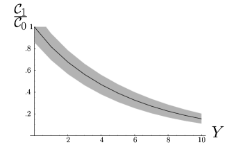
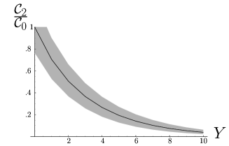
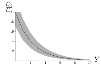
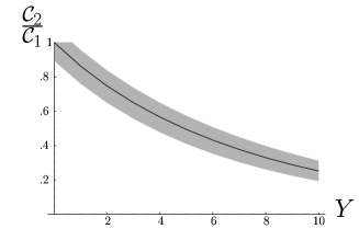
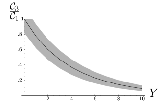
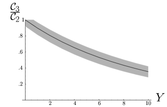
Figure 9: Different ratios of the coefficients $\mathcal{C}_{n}$ obtained using a collinearly resummed BFKL kernel. The gray band reflects the uncertainty in $s_{0}$ and in the renormalization scale $\mu$.

For the differential cross section we also provide results at large Y in Fig. 10. Our calculation is not exact and we partially estimated the uncertainty associated to the running of the coupling and to the sector of the NLO Mueller–Navelet jet vertex originating from the splitting functions, which can be easily read off from Refs. [5]. It turns out that the effect on the overall normalization can be large, as it has been shown in Ref. [25], but the influence in the ratios that we consider here is only of the order of a few percent. We also estimate the uncertainty in our choice of rapidity variable Y by varying our choice of Regge scale $s_{0}=p_{1}p_{2}$ by a factor of 2. We also varied the renormalization scale $\mu$ by the same factor, and represented the uncertainty stemming from these two sources by gray bands in Fig. 9 and Fig. 10.

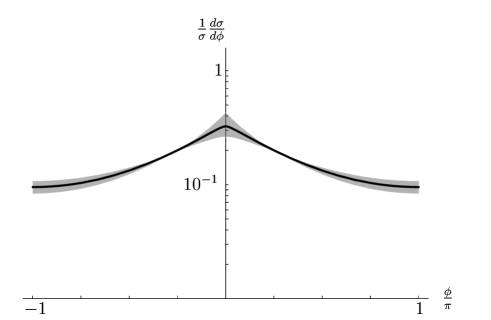
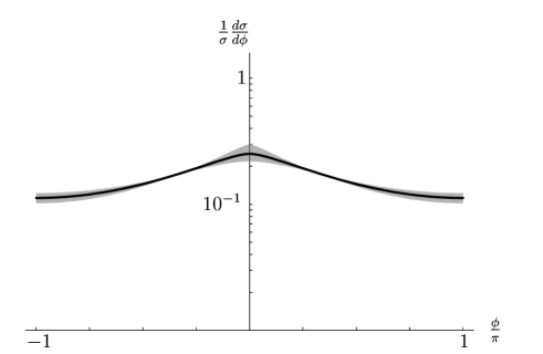
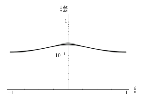
Figure 10: $\frac{1}{\sigma}\frac{d\sigma}{d\phi}$ in our resummation scheme for rapidities Y = 7, 9, 11 from top to bottom. The gray band reflects the uncertainty in $s_{0}$ and in the renormalization scale $\mu$.

5 Conclusions

We have presented a detailed analytic study of the effects of NLO corrections to the BFKL kernel in the description of azimuthal angle decorrelations for Mueller–Navelet jets in hadron colliders. From the technical point of view we found that the intercepts for conformal spins other than zero have good convergence properties and are not largely modified when a collinear resummation is performed. The zero conformal spin component does need of this resummation to get stable results. It is possible to reduce the uncertainties present in our analytic study by using Monte Carlo techniques [26] and work is in progress in this direction [27].

From the phenomenological side we have performed comparisons to the only available data related to this observable, which were extracted at the Tevatron many years ago. As the rapidity differences between the two tagged jets in the D$\emptyset$ experiment were not very large it is natural to think that a fix order calculation would do a better job in fitting the data than a BFKL resummation. Indeed we find that our results improve with respect to the LO BFKL predictions but still show too much azimuthal angle decorrelation. We would like to encourage the experimental study of this observable at the LHC at CERN with rapidity differences quite larger than the presently available in the literature. This would be very useful to investigate the importance of BFKL effects in multijet production in a hadronic environment. If the available rapidity range is large enough there is a good opportunity to study other jet topologies which could be dominated by multi–Regge kinematics. For these studies the NLO production vertex and techniques developed in Ref. [7, 28] will be very useful.

Acknowledgments

We would like to thank P. Aurenche, J. Bartels, M. Ciafaloni, M. Fontannaz, H. Jung, L. Lipatov and L. Motyka for very interesting discussions. F.S. is supported by the Graduiertenkolleg “Zukünftige Entwicklungen in der Teilchenphysik”.

References

- [1] L. N. Lipatov, Sov. J. Nucl. Phys. 23, 338 (1976); V. S. Fadin, E. A. Kuraev and L. N. Lipatov, Phys. Lett. B 60, 50 (1975), Sov. Phys. JETP 44, 443 (1976), Sov. Phys. JETP 45, 199 (1977); I. I. Balitsky and L. N. Lipatov, Sov. J. Nucl. Phys. 28, 822 (1978), JETP Lett. 30, 355 (1979).
- [2] A. Sabio Vera, Nucl. Phys. B 746 (2006) 1.
- [3] A. H. Mueller, H. Navelet, Nucl. Phys. B 282 (1987) 727.
- [4] V.S. Fadin, L.N. Lipatov, Phys. Lett. B 429, 127 (1998); G. Camici, M. Ciafaloni, Phys. Lett. B 430, 349 (1998).
-
[5]
J. Bartels, D. Colferai, G. P. Vacca, Eur. Phys. J. C 24 (2002) 83;
J. Bartels, D. Colferai, G. P. Vacca, Eur. Phys. J. C 29 (2003) 235. - [6] G. P. Salam, JHEP 9807, 019 (1998).
- [7] F. Schwennsen, DESY-THESIS-2007-001 (2007).
- [8] A. V. Kotikov, L. N. Lipatov, Nucl. Phys. B 582 (2000) 19.
- [9] C. R. Schmidt, Phys. Rev. D 60 (1999) 074003; J. R. Forshaw, D. A. Ross, A. Sabio Vera, Phys. Lett. B 455 (1999) 273; G. Chachamis, M. Lublinsky, A. Sabio Vera, Nucl. Phys. A 748 (2005) 649.
- [10] A. Sabio Vera, Nucl. Phys. B 722 (2005) 65.
- [11] S. Catani, B. R. Webber, G. Marchesini, Nucl. Phys. B 349 (1991) 635.
- [12] Y. L. Dokshitzer, V. A. Khoze, S. I. Troian, Phys. Rev. D 53 (1996) 89.
- [13] M. Ciafaloni, D. Colferai, G. P. Salam, A. M. Stasto, Phys. Rev. D 68 (2003) 114003.
- [14] B. Abbott et al., Phys. Rev. Lett. 84 (2000) 5722.
- [15] J. R. Andersen, V. Del Duca, S. Frixione, C. R. Schmidt, W. J. Stirling, JHEP 0102 (2001) 007.
- [16] V. Del Duca, C. R. Schmidt, Phys. Rev. D 49 (1994) 4510.
- [17] W. J. Stirling, Nucl. Phys. B 423 (1994) 56.
- [18] L. H. Orr, W. J. Stirling, Phys. Rev. D 56 (1997) 5875.
- [19] J. Kwiecinski, A. D. Martin, L. Motyka, J. Outhwaite, Phys. Lett. B 514 (2001) 355.
- [20] A. Sabio Vera, F. Schwennsen, hep-ph/0611151.
- [21] S. Abachi et al., Phys. Rev. Lett. 77 (1996) 595.
- [22] W. T. Giele, E. W. N. Glover, D. A. Kosower, Nucl. Phys. B 403 (1993) 633.
- [23] G. Marchesini, B. R. Webber, G. Abbiendi, I. G. Knowles, M. H. Seymour, L. Stanco, Comput. Phys. Commun. 67 (1992) 465.
- [24] C. L. Kim, FERMILAB-THESIS-1996-30.
- [25] O. Kepka, C. Royon, C. Marquet, R. Peschanski, hep-ph/0612261.
- [26] J. R. Andersen, A. Sabio Vera, Phys. Lett. B 567 (2003) 116; Nucl. Phys. B 679 (2004) 345; Nucl. Phys. B 699 (2004) 90; JHEP 0501 (2005) 045.
- [27] A. Sabio Vera, P. Stephens, hep-ph/0611122.
- [28] J. Bartels, A. Sabio Vera, F. Schwennsen, JHEP 0611 (2006) 051; hep-ph/0611137.