Searching for the Higgs boson

Abstract

These lectures on Higgs boson collider searches were presented at TASI 2006. I first review the Standard Model searches: what LEP did, prospects for Tevatron searches, the program planned for LHC, and some of the possibilities at a future ILC. I then cover in-depth what comes after a candidate discovery at LHC: the various measurements one has to make to determine exactly what the Higgs sector is. Finally, I discuss the MSSM extension to the Higgs sector.

I Introduction

Despite all the remarkable progress made early in the 21^st century formulating possible explanations for the weakness of gravity relative to the other forces, the nature of dark matter (and dark energy), what drove cosmological inflation, why neutrino masses are so small, and what might unify the gauge forces, we still have not yet answered the supposedly more readily accessible problem of electroweak symmetry breaking. Just what, exactly, gives mass to the weak gauge bosons and the known fermions? Is it weakly-coupled and spontaneous, involving fundamental scalars, or strongly-coupled, involving composite scalars? Is the flavor problem linked? Do we discover the physics behind dark matter (and its mass), gauge unification and flavor at the same time? Or are those disconnected problems?

Our starting point is unitarity, the conservation of probability: the weak interaction of the Standard Model (SM) of particle physics violates it at about 1 TeV LQT . The theory demands at least one new propagating scalar state with gauge coupling to weak bosons to keep this under control. The same problem holds for fermion–boson interactions Appelquist:1987cf ; Maltoni:2001dc ; Dicus:2004rg ; Dicus:2005ku , only at much higher energy, so is generally less often discussed. While the variety of explanations for electroweak symmetry breaking (EWSB) is vast, what we call the Standard Model (SM) assumes the existence of a single fundamental scalar field which spontaneously acquires a vacuum expectation value to generate all fermion and boson masses. It is a remarkably compact and elegant explanation, simple in the extreme. Yet while it tidies up the immediate necessities of the SM, it suffers from glaring theoretical pathologies that drive much of the model-building behind more ambitious explanations.

Numerous lectures and review articles already exist, covering the SM Higgs sector and the minimal supersymmetric (MSSM) extension HHG ; Djouadi ; Spira:1997dg ; gunion_haber , which are useful both for learning nitty-gritty theoretical details and serving as formulae references. These lectures are instead a crash-course tour of theory in practical application: previous, present and planned Higgs searches, what happens after a candidate Higgs discovery, and an overview of MSSM Higgs phenomenology as a perturbation of that for SM Higgs. They are not comprehensive, but do provide a solid grounding in the basics of Higgs hunting. They should be read only after one has become intimate with the SM Higgs sector and its underlying theoretical issues. Within TASI 2006, this means you should already have studied Sally Dawson’s lectures. After both of these you should also be able to explain to your friends how we look for a Higgs boson at colliders (if they care), how to confirm it’s a Higgs and figure out what variety it is (since we care), and describe how some basic extensions to the SM Higgs sector behave as a function of their parameter space (nature might not care for the SM).

Herein I’ll assume that nature prefers fundamental scalars and spontaneous symmetry breaking. This is a strong bias, but one that provides a solid framework for phenomenology. The ambitious student who wants to really learn all the varieties of EWSB should also study strong dynamics SD , dimensional deconstruction Arkani-Hamed:2001nc , extra-dimensional Higgsless constructions Simmons:2006iw and the Little Higgs LH-reviews and Twin Higgs mechanisms Chacko:2005pe . In many of these classes of theories the Higgs sector appears to be very SM-like, but in some no Higgs appears and one instead would pay great attention to weak boson scattering around a TeV.

II Collider searches for the Standard Model Higgs

Even though the SM Higgs sector doesn’t explain flavor (why all the fermion masses are scattered about over 12 orders of magnitude in energy) and has a disconcerting radiative stability problem that surely must involve new physics beyond the SM, it’s a suitable jumping-off point for formulating Higgs phenomenology. That is, the study of physical phenomena associated with a theory, exploring the connection between theory and experiment. Without this connection, experiments would not make sense and theory would flail about, untested. To survey SM Higgs collider physics we need to recall a few fundamentals about the SM Higgs boson.

• The Higgs boson unitarizes weak boson scattering, $VV\to VV$, so its interaction with weak bosons is very strictly defined to be the electroweak gauge coupling times the vacuum expectation value (vev); i.e., proportional to the weak boson masses.

• The Higgs also unitarizes $VV\to f\bar{f}$ scattering, so its fermion couplings (except $\nu_{i}$) are proportional to the fermion mass, with a strictly defined universal coefficient.

• Because of the coupling strengths, the Higgs is dominantly produced by or in association with massive particles (including loop-induced processes, as we’ll see in Sec. II.1.1), and prefers to decay to the most massive particles kinematically allowed.

• The Higgs boson mass itself is a free parameter, but influences EW observables, so we can fit EW precision data to make a prediction for its mass.

We may thus define the SM Higgs sector by its vacuum expectation value, $v$, measured via $M_{W}$, $G_{F}$, etc., and the known electroweak gauge couplings; 9 Yukawa couplings (fermion mass parameters, ignoring neutrinos and CKM mixing angles); and one free parameter, $M_{H}$.

Prior to the Large Electron Positron (LEP) collider era starting around 1990, Higgs searches involved looking for resonances amongst the low energy hadronic spectra in $e^{+}e^{-}$ collisions. These were in fact non-trivial searches, mostly involving decays of hadrons to Higgs plus a photon, but are generally regarded as comprehensive and set a lower mass bound of $M_{H}\gtrsim 3$ GeV.

Higgs hunting in the 1990s was owned by LEP, an $e^{+}e^{-}$ collider at CERN which steadily marched up in energy over the decade. It found no Higgs bosons. Attention then turned to the long-delayed Tevatron Run II program, proton–antiproton collisions at 2 TeV, which got off to a shaky start but is now performing splendidly. It so far sees nothing Higgs-like, either, but has not yet gathered enough data to be able to say much. The proton–proton Large Hadron Collider (LHC) at CERN is also many years behind schedule, but its construction is now nearing completion and we may expect physics data within a few years.

Our survey begins with LEP from a historical perspective and some general statements about Higgs boson behavior as a function of its mass. Next we turn our attention to the ongoing Tev2 search, for which the prospects hinge critically on machine performance. Then we delve into the intricacies of LHC Higgs pheno, which is far more complicated than either LEP or Tevatron, yet essentially guarantees an answer to our burning questions.

II.1 The LEP Higgs search

An obvious question to ask is, can we produce the Higgs directly in $e^{+}e^{-}$ collisions? We could then probe Higgs masses up to our machine energy, which for LEP-II eventually reached 209 GeV. Recalling that the Higgs–electron coupling is proportional to the electron mass, which is quite a bit smaller than the electroweak vev of 246 GeV, the coupling strength is about $1.5\times 10^{-6}$, or teeny-tiny in technical parlance. A quick calculation reveals that it would take about 4 years running full-tilt to produce just one Higgs boson. This one event would have to be distinguished from the general scattering cross section to fermion pairs in the SM, which is beyond hopeless.

Instead, we think of what process involves something massive, with vastly larger Higgs coupling, so that the interaction rate is large enough to produce a statistically useful number of Higgs bosons. The two obvious possibilities are $e^{+}e^{-}\to W^{+}W^{-}H$ (two $W$’s required for charge conservation) and $e^{+}e^{-}\to ZH$. The first process will obviously have less reach in $M_{H}$ as the two $W$ bosons require far more energy than a single $Z$ boson to produce. LEP Higgs searches therefore focused on the latter process, shown as a Feynman diagram in Fig. 1: the electron and positron annihilate to form a virtual $Z$, far above its mass shell, which returns on-shell by spitting off a Higgs boson. This process is generically known as Higgsstrahlung, analogous to bremsstrahlung radiation. Both the Higgs and $Z$ immediately decay to an asymptotic final state of SM particles. For the Higgs this is preferentially to the most massive kinematically-allowed pair, while $Z$ decays are governed by the fermion gauge couplings. In brief, the $Z$ decays $70\%$ of the time to jets, $20\%$ of the time invisibly (to neutrinos, which the detectors can’t see), and about $10\%$ to charged leptons, which are the most distinctive, “clean” objects in a detector.

Figure 1: Feynman diagram for the process $e^{+}e^{-}\to ZH$ with subsequent Higgs and $Z$ boson decays to fermion pairs. All LEP Higgs searches were based primarily on this process, with various fermion combinations in the final state composing the different search channels.

II.1.1 Momentary diversion: Higgs decays

What, precisely, are the Higgs branching ratios (BRs)? To find these, we first need the Higgs partial widths; that is, the inverse decay rates to each final state kinematically allowed. Everyone should calculate these once as an exercise.

Let’s start with the easiest case: Higgs decay to fermion pairs, which is a very simple matrix element. The general result at tree-level is:

$$\Gamma_{f\bar{f}}\;=\;\frac{N_{c}\,G_{F}\,m^{2}_{f}\,M_{H}}{4\sqrt{2}\,\pi}\,\beta^{3}\qquad{\rm where}\;\;\beta\,=\,\sqrt{1-\frac{4m^{2}_{f}}{M^{2}_{H}}}$$ (1)

One factor of the fermion velocity $\beta$ comes from the matrix element and two factors come from the phase space. I emphasize that this is at tree-level because there are significant QCD corrections to colored fermions. The bulk of these corrections are absorbed into a running mass (see Ref. Spira:1997dg ). For calculations we should always use $m_{q}(M_{H})$, the quark mass renormalized to the Higgs mass scale, rather than the quark pole mass. Programs such as hdecay Djouadi:1997yw will calculate these automatically given SM parameter inputs, greatly simplifying practical phenomenology.

Note that the partial width to fermions is linear in $M_{H}$, modulo the cubic fermion velocity dependence, which steepens the ascent with $M_{H}$ near threshold. Partial widths for various Higgs decays are shown in Fig. 2. While the total Higgs width above fermion thresholds grows with Higgs mass, Higgs total widths below $W$ pair threshold are on the order of tens of MeV – quite narrow. The only complicated partial width to fermions is that for top quarks, for which we must treat the fermions as virtual (at least near threshold) and use the matrix elements to the full six-fermion final state, integrated over phase space. This is slightly more complicated, but easily performed numerically.

Before the decay to top quarks is kinematically allowed, however, the decays to weak bosons turn on. A few $W$/$Z$ widths above threshold the $W$ and $Z$ may be treated as on-shell asymptotic final states, making the partial width calculation easier. We find:

$$\Gamma_{VV}\;=\;\frac{G_{F}M^{3}_{H}}{16\sqrt{2}\pi}\;\delta_{V}\beta\,\biggl{(}1-x_{V}+\frac{3}{4}x^{2}_{V}\biggr{)}\;\;{\rm where}\;\begin{cases}\delta_{W,Z}\,=\,2,1\\ \beta\,=\,\sqrt{1-x_{V}}\\ x_{V}\,=\,\frac{4M^{2}_{V}}{M^{2}_{H}}\end{cases}$$ (2)

The factor of $\beta$ comes from phase space, while the matrix elements give the more complicated function of $x_{V}$. The partial width is dominantly cubic in $M_{H}$, although the factors of beta and $x_{V}$ enhance this somewhat near threshold, as in the fermion case. We can see this in Fig. 2: the partial widths to $VV$ gradually flatten out to cubic behavior above threshold. The reason for this stronger $M_{H}$ dependence compared to fermions is that a longitudinal massive boson wavefunction is proportional to its energy in the high-energy limit, which enhances the coupling by a factor $E/M_{V}$. (Recall that it is this property of massive gauge bosons that requires the Higgs, lest their scattering amplitude rise as $E^{2}/M_{V}^{2}$, violating unitarity. The Higgs in fact generates the longitudinal modes.) This much stronger dependence on $M_{H}$ leads to a very rapid total width growth with $M_{H}$, which reaches 1 GeV around $M_{H}=190$ GeV. We’ll return to this when discussing Higgs couplings measurements in Sec. III.3. The bottom line is that bosons “win” compared to fermions. Thus, even though the top quark has a larger mass than $W$ or $Z$, it cannot compete for partial width and thus BR. Note that the partial widths to $VV$ are non-trivial below threshold: the $W$ and $Z$ are unstable and therefore have finite widths; they may be produced off-shell. The Higgs can decay to these virtual states because its coupling is proportional to the daughter pole masses (or, in the case of quarks, the running masses), not the virtual $q^{2}$, which can be much smaller. Below threshold the analytical expressions are known H_VV_OFS (see Ref. Djouadi for a summary), but are not particularly insightful to derive as an exercise.

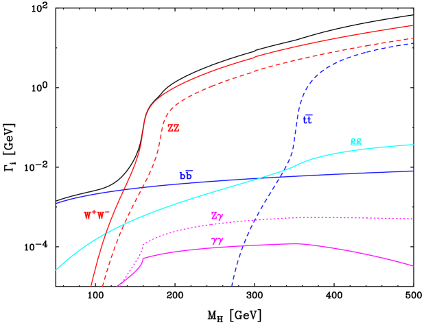
Figure 2: Select Standard Model Higgs boson partial widths, as a function of mass, $M_{H}$. Individual partial widths are labeled, while the total width (sum of all partial widths, some minor ones not shown) is the black curve. Widths calculated with hdecay Djouadi:1997yw .

The astute reader will have noticed by now that Fig. 2 contains curves for Higgs partial widths to massless final states! (Have another look if you didn’t notice.) We know the Higgs couples to particles proportional to their masses, so this requires some explanation. Recall that loop-induced transitions can occur at higher orders in perturbation theory. Such interactions typically are important to calculate only when a tree-level interaction doesn’t exist. They are responsible for rare decays of various mesons, for instance, and are in some cases sensitive to new physics which may appear in the loop. Here, we consider only SM particles in the loop. Which ones are important? Recall also once again that the Higgs boson couples proportional to particle mass. Thus, the top quark and EW gauge bosons are most important. For $H\to gg$, then, that means only the top quark, while for $H\to\gamma\gamma$ it is both the top quark and $W$ loops (there is no $ZZ\gamma$ vertex). The $H\to gg$ expression (for the Feynman diagram of Fig. 3) is Rizzo:1979mf :

Figure 3: Feynman diagram for the loop-induced process $H\to gg$ in the SM. All quarks enter the loop, but contribute according to their Yukawa coupling squared (mass squared). In the SM, only the top quark is important.

$$\Gamma_{gg}\;=\;\frac{\alpha^{2}_{s}G_{F}M_{H}^{3}}{16\sqrt{2}\,\pi^{3}}\bigg{|}\sum\limits_{i}\tau_{i}\bigl{[}1+(1-\tau_{i})f(\tau_{i})\bigr{]}\bigg{|}^{2}$$ (3)

$${\rm with}\quad\tau_{i}\,=\,\frac{4m^{2}_{f}}{M^{2}_{H}}\quad{\rm and} f(\tau)\,=\,\begin{cases}\bigl{[}\sin^{-1}\sqrt{1/\tau}\bigr{]}^{2}&\tau\geq 1\\ -\frac{1}{4}\bigl{[}\ln\frac{1+\sqrt{1-\tau}}{1-\sqrt{1-\tau}}-i\pi\bigr{]}^{2}&\tau<1\end{cases}$$ (4)

which is for a general quark in the loop with SM Yukawa coupling. It’s easy to see that in the SM the $b$ quark contribution, which is second in size to that of the top quark, is inconsequential. Remember to use the running mass $m_{f}(M_{H})$ to take into account the largest QCD effects. When you derive this expression yourself as an exercise, take care to solve the loop integral in $d>4$ dimensions, otherwise you miss a finite piece. The $H\to\gamma\gamma,Z\gamma$ expressions have a similar form H_gamgam , but with two loop functions, since it can also be mediated a $W$ boson loop (which interferes destructively with the top quark loop!):

$$\Gamma_{\gamma\gamma}\;=\;\frac{\alpha^{2}G_{F}M_{H}^{3}}{128\sqrt{2}\,\pi^{3}}\bigg{|}\sum\limits_{i}N_{c,i}Q_{i}^{2}F_{i}\bigg{|}^{2}$$ (5)

$$F_{1}\,=\,2+3\tau[1+(2-\tau)f(\tau)]\,,\;F_{1/2}\,=\,-2\tau[1+(1-\tau)f(\tau)]\,,\;F_{0}\,=\,\tau[1-\tau f(\tau)]$$ (6)

where $N_{c,i}$ is the number of colors, $Q_{i}$ the charge, and $F_{j}$ the particle’s spin.

Now look again more closely at Fig. 2. The important feature to notice is that these loop-induced partial widths are ostensibly proportional to $M_{H}^{3}$, like the decays to gauge bosons. However, the contents of the brackets, specifically the $f(\tau_{i})$ function, can alter this in non-obvious ways. For $H\to gg$, Fig. 2 shows a slightly more than cubic dependence at low masses, leveling of to approximately $M_{H}^{3}$, and flattening out to approximately quadratic a bit above the top quark pair threshold. We see from Eq. 3 that the functional form changes at that threshold, albeit fairly smoothly, by picking up a constant imaginary piece when the top quarks in the loop can be on-shell.

The partial widths to $\gamma\gamma$ and $Z\gamma$ behave very differently than $gg$. For $M_{H}$ below $W$ pair threshold, the interference between top quark and $W$ loops produces an extremely sharp rise with $M_{H}$, which transitions to something slightly more than linear in $M_{H}$ at $W$ pair threshold where the $W$ bosons in the loop go on-shell. There is is a smoother transition at the top quark pair threshold, where they can similarly go on-shell. The $\gamma\gamma$ and $Z\gamma$ partial widths behave differently because of the different $t\bar{t}\gamma$ and $t\bar{t}Z$ couplings: the partial width to $Z\gamma$ at large $M_{H}$ is almost a constant, but falls off for $\gamma\gamma$ almost inverse cubic in $M_{H}$.

Once we’ve calculated all the various possible partial widths, we sum them up to find the Higgs total width. Each BR is then simply the ratio $\Gamma_{i}/\Gamma_{tot}$. These are shown in Fig. 4; note the log scale. If it wasn’t obvious from the partial width discussion, it should be now: near thresholds, properly including finite width effects can be very important to get the BRs correct. Observe how the BR to $WW^{*}$ (at least one $W$ is necessarily off-shell) is $50\%$ at $M_{H}=140$ GeV, 20 GeV below $W$ pair threshold. BR($H\to b\bar{b}$)$\sim$BR($H\to W^{+}W^{-}$) at $M_{H}=136$ GeV.

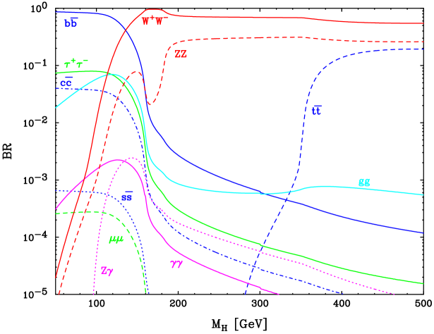
Figure 4: Select Standard Model Higgs boson branching ratios as a function of mass, $M_{H}$ Djouadi:1997yw . The Higgs prefers to decay to the most massive possible final state. The ratio of fermionic branching ratios are proportional to fermion masses squared, modulo color factors and radiative corrections.

II.1.2 A brief word on statistics – the simple view

Now that we understand the basics of Higgs decay, and production in electron-positron collisions, we should take a moment to consider statistics. The reason we must resort to statistics is that particle detectors are imperfect instruments. It is impossible to precisely measure the energy of all outgoing particles in every collision. The calorimeters are sampling devices, which means they don’t capture all the energy; rather they’re calibrated to give an accurate central value at large statistics, with some Gaussian uncertainty about the mean for any single event. Excess energy can also appear, due to cosmic rays, beam–gas or beam secondary interactions. Quark final states hadronize, resulting in the true final state in the detector (a jet) being far more complicated and difficult even to identify uniquely. The electronics can suffer hiccups, and software always has bugs, leading to imperfect analysis. Thus, we would never see two or three events at precisely the Higgs mass of, say, 122.6288… GeV, and pop the champagne. Rather, we’ll get a distribution of masses and have to identify the central value and its associated uncertainty.

In any experiment, event counts are quantum rolls of the dice. For a sufficient number of events, they also follow a Gaussian distribution about the true mean:

$$f(x;\mu,\sigma)\;=\;\frac{1}{\sigma\sqrt{2\pi}}\>exp\biggl{(}-\frac{(x-\mu)^{2}}{2\sigma^{2}}\biggr{)}$$ (7)

The statistical uncertainty in the rate then goes as $1/\sqrt{N}$, where $N$ is the number of events. This is “one sigma” of uncertainty: $68.2\%$ of identically-conducted experiments would obtain $N$ within $\sigma\approx\pm\sqrt{N}$ about $\mu=N_{\rm true}$, representing the true cross section. Fig. 5 shows the fractional probabilities for various “sigma”, or number of standard deviations from the true mean. To claim observation of a signal deviating from our expected background, we generally use a $5\sigma$ criteria for discovery. This means, if systematic errors have been properly accounted for, that there is only a $0.00006\%$ chance that the signal is due to a statistical fluctuation. However, this threshold is subjective, and you will often hear colleagues take $4\sigma$ or even $3\sigma$ deviations seriously. Since particle physics has seen dozens of three sigma deviations come and go over the decades, I would encourage you to regard $3\sigma$ as “getting interesting”, and $4\sigma$ as “pay close attention and ask lots of questions about systematics”.

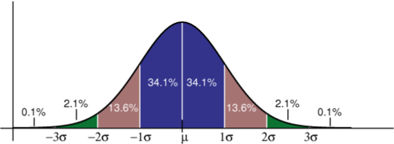
Figure 5: Gaussian distribution about a mean $\mu$, showing the fractional probability of events within one, two and three standard deviations of the mean.

Because SM processes can produce the same final state as any $ZH$ combined BR, we must know accurately what the background rate is for each signal channel (final state) and how it is distributed in invariant mass, then look for a statistically significant fluctuation from the expected background over a fixed window region. The size of the window is determined by detector resolution: the better the detector, the narrower the window, so the smaller the background, yielding a better signal-to-background rate. Generally, the window is adjusted to accept one or two standard deviations of the hypothesized signal ($68$–$95\%$).

Analyses are then defined by two different Gaussians: that governing how many signal (and background) events were produced, and that parameterizing the detector’s measurement abilities. The event count $N$ in our above expression is the actual number of events observed, in an experiment. But in performing calculations ahead of time for expected signal and background, it is variously taken as just $B$, the number of background events expected, or $S+B$, expected signal included, depending on the relative sizes of $S$ and $B$. For doing phenomenology, trying to decide which signals to study and calculate more precisely, the distinction is often ignored.

The statistical picture I’ve outlined here is quite simplified. Not all experiments have sufficient numbers of events to describe their data by Gaussians – Poisson statistics may be more appropriate. (An excellent text on statistics for HEP is Ref. Lyons:1986em .) Not all detector effects are Gaussian-distributed. Nevertheless, it gets across the main point: multiple sources of randomness introduce a level of uncertainty that must be parameterized by statistics. Only when the probability of a random background fluctuation up or down to the observed number of events is small enough, perhaps in some distribution, can signal observation be claimed. Exactly where this line lies is admittedly a little hazy, but there’s certainly a point of several sigmas at which everybody would agree.

II.1.3 LEP Higgs data and results

Now to the actual LEP search. Electrons and positrons have only electroweak interactions, so backgrounds and a potential Higgs signal are qualitatively of the same size. (We’ll see shortly in Sec. II.2 how this is not so at a hadron collider, which has colored initial states.) LEP thus had the ability to examine almost all $Z$ and $H$ decay combinations: $b\bar{b}jj$, $b\bar{b}\ell^{+}\ell^{-}$, $b\bar{b}\nu\bar{\nu}$, $\tau^{+}\tau^{-}jj$, $jjjj$, etc. The largest of these is $b\bar{b}jj$, as it combines the largest BRs of both the $Z$ and $H$. It’s closely followed by $b\bar{b}\nu\bar{\nu}$, since a $Z$ will go to neutrinos $20\%$ of the time. Neutrinos are missing energy, however, so not precisely measured, making it possible that any observed missing energy didn’t in fact come from a $Z$. Jets are much less well-measured than leptons, so a narrower mass window can be used for the $Z$ in $b\bar{b}\ell^{+}\ell^{-}$ events than $b\bar{b}jj$; the smaller backgrounds in the narrower window might beat the smaller statistics of the leptonic final state.

The exact details of each LEP search channel are not so important, as lack of observation means we’re more interested in channels’ signal and background attributes at hadron colliders. For these lectures I just present the final LEP result combining all four experiments. The interested student should read Eilam Gross’ “Higgs Statistics for Pedestrians”, which goes into much more depth, and with wonderful clarity Gross:2002wg .

The money plot is shown in Fig. 6. It shows the expected confidence level (CL) for the signal+background hypothesis as a function of Higgs mass. The thin solid horizontal line at CL=0.05 signifies a $5\%$ probability that a true signal together with the background would have fluctuated down in number of events to not be discriminated from the expected background. The green and yellow regions are the $1\sigma$ and $2\sigma$ expected uncertainty bands as a function of $M_{H}$, taking into account all sources of uncertainty, calculational as well as detector effects. Where the central value (dashed curve) crosses 0.05 defines the $95\%$ CL expected exclusion (lower mass limit). This is essentially the available collision energy minus the $Z$ mass minus a few extra GeV to account for the $Z$ finite width – it may be produced slightly off-shell with some usable rate. The solid red curve is the actual experimental result, which is slightly above the experimental result everywhere, meaning that the experiments gathered a couple more events than expected in the 115-116 GeV mass bin.

The end of LEP running involved a certain amount of histrionics. At first, the number of excess event at the kinematic machine limit was a few, but more careful analyses removed most of these. For example, one particularly notorious event originally included in one experiment’s analysis had more energy than the beam delivered. Another experiment removed a candidate event because some of the outgoing particles traveled down a poorly-instrumented region of the detector which was not normally used in analysis. The final, most credible enumeration was one candidate event in one experiment, show in Fig. 7.

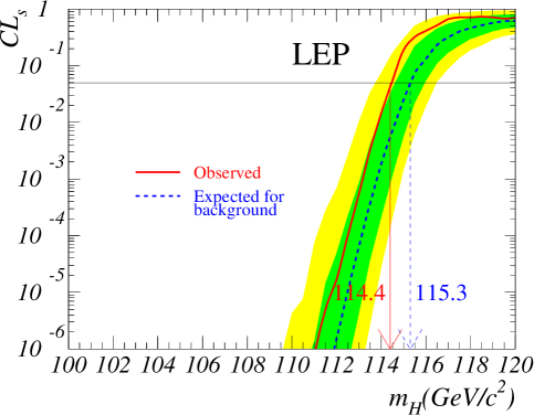
Figure 6: Four-experiment combined result of the LEP Standard Model Higgs search. No signal was observed, establishing a lower limit of 114.4 GeV. See text of Ref. Gross:2002wg for explanation.

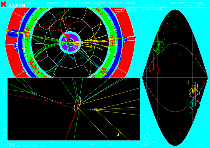
Figure 7: Event display of an interesting candidate $Z\to jj$, $H\to b\bar{b}$ event in the Aleph detector at the end of LEP-II running and at the machine’s kinematic limit ALEPH_H-cand_event .

II.2 Prospects at Tevatron

With the end of the LEP era, all eyes turned to Run II of the upgraded Fermilab Tevatron. Its energy increased from 1.8 to 1.96 GeV, and is expected to gather many tens of times the amount of data in Run I. Higgs-hunting hopes were high Carena:2000yx , although it was clear that the machine and both detectors have to perform exceptionally well to have a chance, as Tevatron’s Higgs mass reach will not be all that great, and will have significant observability gaps in the mass region expected from precision EW data.

To understand the details and issues, we first need to identify how a Higgs boson may be produced in proton-antiproton collisions. Like the electron, the light quarks have too small a mass (Yukawa coupling) to produce a Higgs directly with any useful rate, discernible against the large QCD backgrounds produced in hadron collisions. Quarks may annihilate, however, to EW gauge bosons, which have large coupling to the Higgs; and likewise to a top quark pair. Incoming quarks may also emit a pair of gauge bosons which fuse to form a Higgs, a process known as weak boson fusion (WBF). But high energy protons also possess a large gluon content; recall that gluons have a loop-induced coupling to the Higgs. Fig. 8 displays Feynman diagrams for all four of these processes at hadron colliders. The questions are, what are their relative sizes, and what are their backgrounds? Because of the partonic nature of hadron collisions, the Higgs couplings are not enough to tell us the relative sizes; we also need to take into account incoming parton fluxes and final state phase space – single Higgs production is much less greedy than $t\bar{t}H$ associated production, for instance. In addition, the internal propagator structure of the processes is important: $WH$,$ZH$ bremsstrahlung are $s$-channel suppressed, but no other process is.

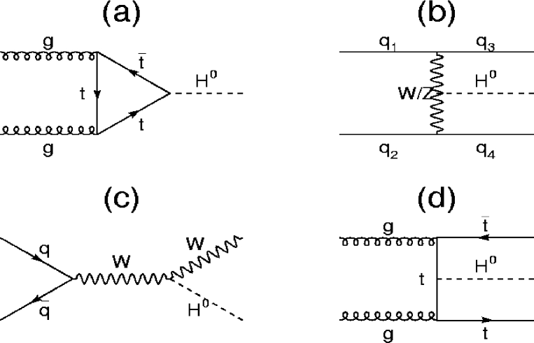
Figure 8: Feynman diagrams for the four dominant Higgs production processes at a hadron collider.

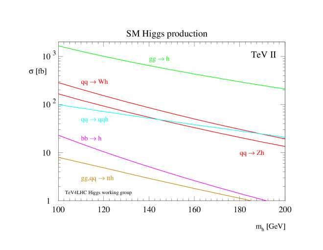
Figure 9: Cross sections for Higgs production in various channels at Tevatron Run II ($\sqrt{s}=2$ TeV). Note the log scale. Figure from the Tev4LHC Higgs working group Hahn:2006my .

The various rates, updated in 2006 with the latest theoretical calculations Hahn:2006my ; Aglietti:2006ne , are shown in Fig. 9 for a light SM Higgs boson. Students not already familiar with hadron collider Higgs physics will probably be surprised to learn that $gg\to H$, gluon fusion Higgs production, dominates at Tevatron energy. This is partly because the coupling is actually not all that small, partly because high-energy protons contain a plethora of gluons, and partly because there is no propagator suppression, and much less phase space suppression, compared to other processes. Higgsstrahlung (Fig. 8(c)) is still important at Tevatron, analogous to LEP. Note that the smaller cross sections have more complicated final states, therefore potentially less background, and possibly distinctive kinematic distributions that could assist in separating a signal from the background. It’s not obvious that the largest rate is the most useful channel! Considering that the Higgs decays predominantly to different final states as a function of its mass, it’s also not obvious that the optimal channel at one mass is optimal for all masses. In fact, that’s definitely not the case.

Not knowing the answer, we naturally start by considering the largest cross section times branching ratio, $gg\to H\to b\bar{b}$. Just how large is the background, QCD $pp\to b\bar{b}$ production? Fig. 10 shows a variety of SM cross section for hadron collisions of various energy, and marks off in particular Tevatron and LHC. (The discontinuity in some curves is because Tevatron is $p\bar{p}$ and LHC is $pp$.) We immediately notice that the $b\bar{b}$ inclusive rate is almost nine orders of magnitude larger than inclusive $H\to b\bar{b}$. Of course the background will be smaller in a finite window about the Higgs mass. But jets are not so well-measured, necessitating a fairly large window, $\sim$15–20 GeV either side of the central value. We lose only a few orders of magnitude of the background, taking us from “laughable” to just terminally hopeless.

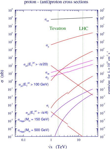
Figure 10: Various SM “standard candle” cross sections at hadron colliders of varying energy, with Tevatron and LHC marked in particular. Note the log scale. Discontinuities are due to the difference between $p\bar{p}$ for Tevatron and $pp$ for LHC. Figure from Ref. Gianotti:2004qs .

The general rule of thumb at hadron collider experiments is to require a final state with at least one high-energy lepton. This means lower backgrounds because the event had at least some EW component, such as a $W$ or $Z$, or came from a massive object, such as the top quark, which is not produced in such great abundance due to phase space suppression.

Tevatron’s Higgs search is rate-limited. We can see this by multiplying the 150 GeV Higgs cross section from Fig. 9 by the expected integrated luminosity of 4–8 fb^-1 during Run II. Because of this, and the very low efficiency of identifying final-state taus in a hadron collider environment (unlike at LEP), Tevatron’s experiments CDF and DØ focus on the $H\to b\bar{b}$ final state where that decay dominates the BR, and Higgsstrahlung to obtain the lepton tag. For larger Higgs masses, where $H\to W^{+}W^{-}$ dominates, gluon fusion Higgs production is the largest rate, but Higgsstrahlung has some analyzing power. To summarize Carena:2000yx :

• 140 GeV: $H\to b\bar{b}$ dominates, so we use:

  • $WH\to\ell^{\pm}\nu b\bar{b}$

  • $ZH\to\ell^{+}\ell^{-}b\bar{b}$

  • $WH$, $ZH\to jjb\bar{b}$

  • $ZH\to\nu\bar{\nu}b\bar{b}$

• 140 GeV: $H\to W^{+}W^{-}$ dominates, so we use:

  • $gg\to H\to W^{+}W^{-}$ (dileptons)

  • $WH\to W^{\pm}W^{+}W^{-}$ ($2\ell$ and $3\ell$ channels)

II.2.1 $VH,H\to b\bar{b}$ at Tevatron

While a lepton tag gets rid of most QCD backgrounds, it doesn’t automatically eliminate top quarks: they decay to $Wb$, thus the event often contains one lepton and two jets, or two leptons and missing energy, in addition to the $b$ jet pair. This is the same final state as our Higgs signal, with either extra jets or transverse energy imbalance. Kinematic cuts help, but because the detectors are imperfect some top quark events will leak through. Jet mismeasurement gives fake missing energy, for example (and is one of the most difficult uncertainties to quantify in a hadron collider experiment). In addition, QCD initial-state radiation from the incoming partons can give extra jets. Thus top quark and Higgs signal events qualitatively become very similar. To control this further the experiments have to look at other observables, such as angular distributions of the $b$ jets and leptons. Other backgrounds to consider are QCD $Wb\bar{b}$ production, weak bosons pairs where one decays to $b\bar{b}$ (and thus has invariant mass close to the Higgs signal window).

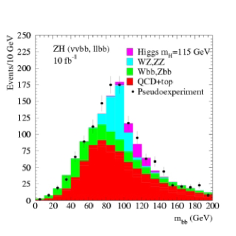
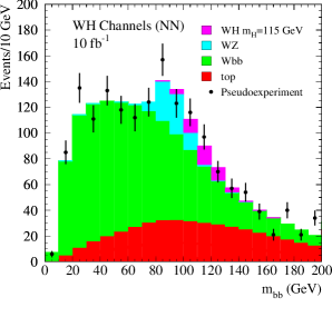
Figure 11: CDF simulations of a 115 GeV signal at Tevatron Run II in $ZH$ (left) and $WH$ (right) Higgsstrahlung production with Higgs decays $H\to b\bar{b}$ and assuming 10 fb^-1 is collected Babukhadia:2003zu .

Fig. 11 shows the results of a CDF simulation study of $WH$ and $ZH$ Higgsstrahlung events at Run II for $M_{H}=115$ GeV (right at the LEP Higgs limit) Babukhadia:2003zu . First note how the top quark pair and diboson backgrounds peak very close to the Higgs mass. Eyeballing the plots and simplistically applying our knowledge of Gaussian statistics, we could easily believe that this could yield a four or five sigma signal, perhaps combined with DØ results. However, carefully observe that the shape of the invariant mass distribution for background alone and with signal are extremely similar: they are both steeply falling; the Higgs signal is not a stand-out peak above a fairly flat background. Therein lies a hidden systematic! This means that we must understand the kinematic-differential shape of the QCD backgrounds to a very high degree of confidence. This is not just knowing the SM background at higher orders in QCD, differentially, but also the detector response. This criticality is not appreciated in most discussions of a potential discovery at Tevatron. It should be obvious that an excess in one of these channels would cause a scramble of cross-checking and probably further theoretical work to ensure confidence, in spite of the statistics alone. We’ll run into this feature again with one of the LHC channels in Sec. II.3.1, but quantified.

CDF has in fact already observed an interesting candidate Higgs event in Run II, in the first few hundred pb^-1. It is in the $ZH\to\nu\bar{\nu}b\bar{b}$ channel (a $b$ jet pair plus missing transverse energy). The event display and key kinematic information are shown in Fig. 12. Given the very low $b$ jet pair invariant mass, it’s much more likely that the event came from EW $ZZ$ or QCD $Zb\bar{b}$ production (cf. Fig. 11). It therefore doesn’t generate the kind of excitement that the handful of events at LEP did. Nevertheless, finding this event was a milestone, showing that CDF could perform such an analysis and find Higgs-like events with good efficiency.

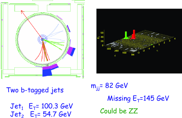
Figure 12: Interesting $bb/\!\!\!p_{T}$ event at CDF in Tevatron Run II CDF8842 .

		Higgs Mass (GeV/$c^{2}$)
Channel	Rate	90	100	110	120	130
	$S$	8.7	9.0	4.8	4.4	3.7
$\ell^{\pm}\nu b\bar{b}$	$B$	28	39	19	26	46
	$S/\sqrt{B}$	1.6	1.4	1.1	0.9	0.5
	$S$	12	8	6.3	4.7	3.9
$\nu\bar{\nu}b\bar{b}$	$B$	123	70	55	45	47
	$S/\sqrt{B}$	1.1	1.0	0.8	0.7	0.6
	$S$	1.2	0.9	0.8	0.8	0.6
$\ell^{+}\ell^{-}b\bar{b}$	$B$	2.9	1.9	2.3	2.8	1.9
	$S/\sqrt{B}$	0.7	0.7	0.5	0.5	0.4
	$S$	8.1	5.6	3.5	2.5	1.3
$q\bar{q}b\bar{b}$	$B$	6800	3600	2800	2300	2000
	$S/\sqrt{B}$	0.10	0.09	0.07	0.05	0.03

Table 1: Predicted signal significances at Tevatron Run II, for one detector and 1 fb^-1, for various $VH,H\to b\bar{b}$ searches, taken from Ref. Carena:2000yx .

Table 1 summarizes the 2000 Tevatron Higgs Working Group Report predictions for Higgsstrahlung reach in Run II Carena:2000yx . The results are quoted for one detector and per fb^-1, hence the rather small significances. CDF and DØ will eventually combine results, giving a factor of two in statistics. However, it’s not known how much data they’ll eventually collect by 2009 or 2010, when LHC is expected to have first physics results and CDF & DØ detector degradation becomes an issue. Fairly low Higgs masses are shown, because when the report was written nobody expected LEP to perform as well as it did, greatly exceeding its anticipated search reach. It should be obvious that a clear discovery would require a large amount of data, combining multiple channels, and the Higgs boson happening to be fairly light; not to mention the QCD shape systematic concern I described earlier (but is not quantified). In spite of this apparent pessimism, however, CDF and DØ seem to be performing modestly better than expected – higher efficiencies for $b$ tagging and phase space coverage, better jet resolution, etc. There is as yet no detailed updated report with tables such as this, but there are some newer graphically-presented expectations I’ll show as a summary.

II.2.2 $gg\to H\to W^{+}W^{-}$ at Tevatron

For $M_{H}\gtrsim 140$ GeV, a SM Higgs will decay mostly to $W$ pairs (cf. Fig. 4), which has a decent rate to dileptons and has very little SM background – essentially just EW $W$ pair production, with some background from top quark pairs where both $b$ jets are lost. This channel has some special characteristics due to how the Higgs decay proceeds. There is a marked angular correlation between the outgoing leptons which differs from the SM backgrounds: they prefer to be emitted together, that is close to the same flight direction in the center-of-mass frame Dittmar:1996ss .

To understand this correlation, consider what happens if the Higgs decays to a pair of transversely-polarized $W$ bosons. For $W$ decays, the lepton angle with respect to the $W^{\pm}$ spin follows a $(1\pm\cos\theta_{\ell^{\pm}})^{2}$ distribution. That is, the positively-charged lepton prefers to be emitted with the $W$ spin, while the negatively-charged lepton prefers to be emitted opposite the $W$ spin. Since the Higgs is a scalar (spin-0), the $W$ spins are anti-correlated, thus the leptons are preferentially emitted in the same direction. For longitudinal $W$ bosons, the lepton follows a $\sin^{2}\theta_{\ell}$ distribution. The $W$ spins are still correlated, however, and the matrix element squared (an excellent exercise for the student) is proportional to $(p_{\ell^{-}}\cdot p_{\nu})(p_{\ell^{+}}\cdot p_{\bar{\nu}})$. Since a charged lepton and neutrino are emitted back-to-back in the $W$ rest frame, this is again maximized for the charged leptons emitted together. This correlation is shown visually by the schematic of Fig. 13. Projected onto the azimuthal plane (transverse to the beam), its efficacy is shown in Fig. 14 by comparison to various backgrounds Carena:2000yx ; Han_H_WW_Tev .

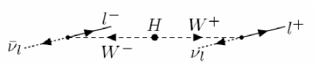
Figure 13: Diagram showing the preferred flight direction of charged leptons in $H\to\ell^{+}\nu\ell^{-}\bar{\nu}$.

Figure 14: Dilepton azimuthal angular correlation for a $H\to W^{+}W^{-}\to\ell^{+}\nu\ell^{-}\bar{\nu}$ signal and its backgrounds. The efficacy of the cut (vertical line) can easily be estimated visually. From the Tevatron Run II Higgs Working Group Report Carena:2000yx .

In addition to this angular correlation, we may also construct a transverse mass ($M_{T}$) for the system, despite the fact that two neutrinos go missing Rainwater:1999sd . We first write down the transverse energy ($p_{T}$) of the dilepton and missing transverse energy ($/\!\!\!E_{T}$) systems,

$$E_{T_{\ell^{+}\ell^{-}}}\;=\;\sqrt{\vec{p}_{T_{\ell^{+}\ell^{-}}}^{2}+m_{\ell^{+}\ell^{-}}^{2}}\;,\qquad/\!\!\!E_{T}\;=\;\sqrt{/\!\!\!\vec{p}_{T}^{2}+m_{\ell^{+}\ell^{-}}^{2}}$$ (8)

where I’ve substituted the dilepton invariant mass $m_{\ell^{+}\ell^{-}}^{2}$ for $m_{\nu\bar{\nu}}^{2}$. This is exact at $H\to WW$ threshold, and is a very good approximation for Higgs masses below about 200 GeV and where this decay mode is open. The $W$ pair transverse mass is now straightforward:

$$M_{T_{WW}}\;=\;\sqrt{(/\!\!\!E_{T}+E_{T_{\ell^{+}\ell^{-}}})^{2}-(\vec{p}_{T_{\ell^{+}\ell^{-}}}+/\!\!\!\vec{p}_{T})^{2}}$$ (9)

This gives a nice Jacobian peak for the Higgs signal, modulo detector missing-transverse-energy resolution, whereas the SM backgrounds tend to be comparatively flat.

Utilizing these techniques gives Tevatron some reach for a heavier Higgs boson, mostly in the mass range $150\lesssim M_{H}\lesssim 180$ GeV, where the BR to $WW$ is significant and the Higgs production rate is not too small.

II.2.3 Tevatron Higgs summary expectations

Tevatron Higgs physics expectations have changed since the 2000 Report, as DØ and CDF have better understood their detectors and made analysis improvements. As yet, the only progress summary is from 2003, shown in Fig. 15. It compares the original Report’s findings, shown by the thick curves, with improved findings for the low-mass region, shown by the thinner lines. However, the new results do not yet include systematic uncertainties, which may be considerable. We should expect some form of a new summary expectation sometime in 2007. A final note on the undiscussed WBF production mode: some study has been done (see Sec. II.C.4 of Ref. Carena:2000yx ), but DØ and CDF both lack sufficient coverage of the forward region to use this mode. This is not the case at LHC.

Run II now has about 1 fb^-1 of analyzed data, and a Higgs search summary progress report is available in Ref. Bernardi:2006fd , which updates each channel’s expectations.

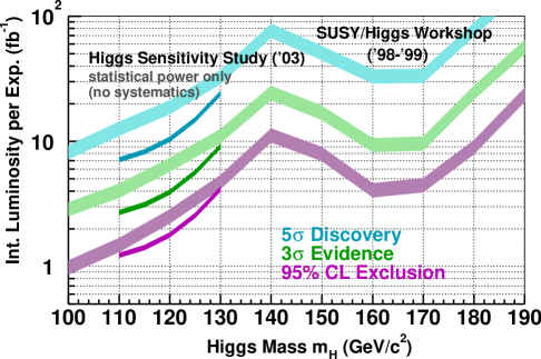
Figure 15: Expected required integrated luminosity per experiment required in Run II to observe a SM Higgs as a function of $M_{H}$ Babukhadia:2003zu .

II.3 Higgs at LHC

Higgs physics at LHC will be similar to that at Tevatron. There is the slight difference that LHC will be $pp$ collisions rather than $p\bar{p}$. The biggest difference, however, is the increased energy, from 2 to 14 TeV. Particle production in the 100 GeV mass range will be at far lower Feynman $x$, where the gluon density is much larger than the quark density. In fact, it’s useful (for Higgs physics) to think of the LHC as a gluon collider to first order. The ratio between gluon fusion Higgs production and Higgsstrahlung is thus larger than at Tevatron. Fig. 16 displays the various SM Higgs cross sections, only over a much larger range of $M_{H}$ – at LHC, large-$M_{H}$ cross sections are not trivially small, compared to at the Tevatron. There are huge QCD corrections to the $gg\to H$ rate (also at Tevatron), but these are now known at NNLO and under control H-NNLO (and included in Fig. 16). They don’t affect the basic phenomenology, however. Knowing that LHC is plans to collect several hundred fb^-1 of data, a quick calculation reveals that the LHC will truly be a Higgs factory, producing hundreds of thousands of light Higgs bosons, or tens of thousands if it’s heavy.

Looking back at Fig. 10, we see that while the Higgs cross section rises quite steeply with collision energy ($gg\to H$ is basically a QCD process), so do important backgrounds like top quark production. The inclusive $b$ cross section is still too large to access to $gg\to H\to b\bar{b}$, but note that the EW gauge boson cross sections do not rise as swiftly with energy. Immediately we realize that channels like $gg\to H\to W^{+}W^{-}$ should have a much better signal-to-background (S/B) ratio. (In fact it suffers from non-trivial single-top quark Kauer:2004fg and $gg\to W^{+}W^{-}$ Binoth_gg-WW backgrounds, but is still an excellent channel for $M_{H}\gtrsim 150$ GeV.) The figure does not show cross sections like $Wb\bar{b}$ or $Zb\bar{b}$, which grow QCD-like and thus become a terminal problem for $WH$ and $ZH$ channels.

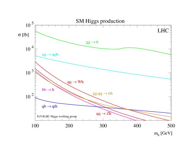
Figure 16: Cross sections for Higgs production in various channels at LHC ($\sqrt{s}=14$ TeV) Hahn:2006my .

Obviously there are a few significant differences between Tevatron and LHC with implications for Higgs physics. We’ll lose access to $WH$ and $ZH$ at low mass, at least for Higgs decay to $b$ jets. What about rare decays, since the production rate is large? The $t\bar{t}H$ cross section is large and would yield a healthy event rate. It’s complexity is distinctive, so one might speculate that perhaps it could be useful. WBF production is also accessible due to better detectors, and likewise its more complex signature is worthy of a look. It will in fact turn out to be perhaps the best production mode at LHC.

As with Tevatron, we need to understand both the signal and background for each Higgs channel we wish to examine. As a prelude to Chapter III, Higgs measurements, at LHC we won’t want to just find the Higgs in one mode. Rather, we’ll want to observe it in as many production and decay modes as possible, to study all its properties, such as couplings.

II.3.1 $t\bar{t}H,H\to b\bar{b}$

Let’s begin by discussing a very complex channel, top quark associated production at low mass, $t\bar{t}H,H\to b\bar{b}$. This was studied early on in the ATLAS TDR ATLAS_TDR and in various obscure CMS notes, and found to be a sure-fire way to find a light Higgs. Fig. 17 shows a schematic of such an event, with multiple $b$ jets from both top quarks and the Higgs, at least one lepton from a $W$ for triggering, and possibly extra soft jets from QCD radiation. The schematic is a bit fanciful in the neatness of separation of the decay products, but is useful to get an idea of what’s going on.

These early studies ATLAS_TDR ; Richter-Was:1999sa ; Drollinger:2001ym ; Abdullin:2005yn were too ambitious, however. The backgrounds to this signal are $t\bar{t}b\bar{b}$ and $t\bar{t}jj$ production, pure QCD processes. The extra ($b$) jets must be fairly energetic, or hard, because the signal is a 100+ GeV-mass object which decays to essentially massless objects. Despite this being a known problem Giele:1990vh , these backgrounds were calculated using the soft/collinear approximation for extra jet emission implemented in standard Monte Carlo tools such as pythia or herwig. This greatly underestimated the backgrounds.

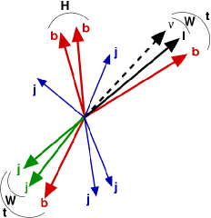
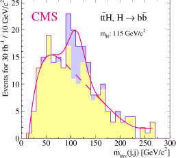
Figure 17: Left: schematic of the outgoing particles in a typical $t\bar{t}H,H\to b\bar{b}$ event at LHC Cammin:2004sz . Right: early CMS study expectations for a $b\bar{b}$ mass peak in such events, for $M_{H}=115$ GeV Drollinger:2001ym ; Abdullin:2005yn .

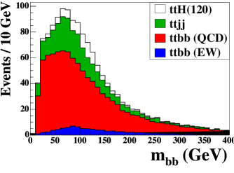
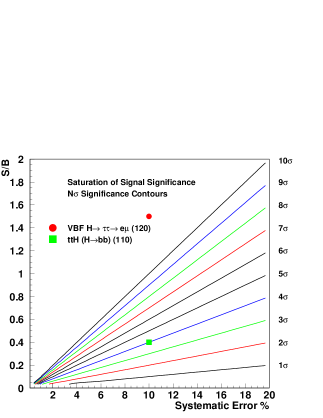
Figure 18: Left: results of a more up-to-date ATLAS studying of $t\bar{t}H,H\to b\bar{b}$ production at LHC, for 30 fb^-1 of data and a Higgs mass of $M_{H}=120$ GeV Cammin:2004sz . The QCD backgrounds were calculated with exact matrix elements rather than in the soft/collinear approximation. Right: maximum achievable signal significance for two LHC Higgs channels as a function of $S/B$ and shape systematic uncertainty $\triangle$ Cranmer , as discussed in the text.

The left panel of Fig. 18 shows the results of a repeated study by ATLAS using a proper background calculation Cammin:2004sz . (Recent CMS studies found similar results, and the new CMS TDR CMS_TDR does not even bother to discuss this channel.) There is no longer any clearly-visible mass peak, and S/B is now about 1/6, much poorer. While the figure reflects only 1/10 of the expected total integrated luminosity at LHC, statistics is not the problem. Rather, it is systematic: uncertainty on the exact shape of the QCD backgrounds.

Therein lies the sleeping dragon. Now is a good time to explain how systematic errors may enter our estimate of signal significance. Our simple formula is modified:

$$\frac{S}{\sqrt{B}}\;\;\to\;\;\frac{S}{\sqrt{B(1+B\triangle^{2})}}\;\;\stackrel{{\scriptstyle{\cal L}\to\infty}}{{\longrightarrow}}\;\;\frac{S/B}{\triangle}$$ (10)

where $\triangle$ is the shape uncertainty in the background, a kind of normalization uncertainty. In the limit of infinite data, if $S/B$ is fixed (which it is), signal significance saturates. The only way around this is to perform higher-order calculations of the background to reduce $\triangle$ (and hope you understand the residual theoretical uncertainties). The right panel of Fig. 18 shows the spectrum of possibilities Cranmer . For the known $10\%$ QCD shape systematic for $t\bar{t}H$, even an infinite amount of data would never be able to grant us more than about a $3\sigma$ significance. This could still potentially be useful for a coupling measurement, albeit poorly, but will not be a discovery channel unless higher-order QCD calculations can improve the situation. Calculating even just $t\bar{t}b\bar{b}$ at NLO is currently beyond the state of the art, but is likely to become feasible within a few years.

While I don’t discuss it here, top quark associated Higgs production does show some promise for the rare Higgs decays to photons. Photons are very clean, well-measured, and the detectors have good rejection against QCD jet fakes. The final word probably hasn’t been written on this, but the CMS TDR CMS_TDR does have updated simulation results which the interested student may read up on.

II.3.2 $gg\to H\to\gamma\gamma$

We’ve just seen that QCD can be a really annoying problem for Higgs hunting at LHC. A logical alternative for a low-mass Higgs is to look for its rare decays to EW objects, e.g. photons. The BR is at about the two per-mille level for a light Higgs, $110\lesssim M_{H}\lesssim 140$ GeV. The LHC will certainly produce enough Higgses, but what are the backgrounds like?

It turns out that the loop-induced QCD process $gg\to\gamma\gamma$ is a non-trivial contribution, but we also have to worry about single and double jet fakes from QCD $j\gamma$ and $jj$ production. This occurs when a leading $\pi^{0}$ from jet fragmentation goes to photons, depositing most of the energy in the EM calorimeter, thereby looking like a real photon. Fortunately, because photons and jets are massless, the invariant mass distribution obeys a very linear $1/m_{\gamma\gamma}$ falloff in our region of interest. The experiments can in that case normalize the background very precisely from the sidebands, where we know there is no Higgs signal. Shape systematics are not much of a concern, thus avoiding the pitfalls of the $t\bar{t}H,H\to b\bar{b}$ case.

Fig. 19 shows the results of an ATLAS study for this channel using 30 fb^-1 of data ATLAS_TDR , 1/10 of the LHC run program or 3 years at low-luminosity running. The exact expectations are still uncertain, mostly due to an ongoing factor of two uncertainty in the fake jet rejection efficiency. A conservative estimate shows that this channel isn’t likely to be the first discovery mode, but would be crucial for measuring the Higgs mass precisely at low $M_{H}$, to about $1\%$ ATLAS_TDR ; CMS_TDR . Photon energy calibration nonlinearity in the detector may be an issue for the ultimate precision, but is generally regarded as minor. We’ll come back to this point in Chapter III on Higgs property measurements.

While I focus here on the SM, keep in mind that because $H\to\gamma\gamma$ is a rare decay, it can be very sensitive to new physics. Recall that the coupling is induced via both top quark and $W$ loops which mostly cancel. Depending on how the new physics alters couplings, or what new particles appear in the loop, the partial width could be greatly suppressed or enhanced. (Anticipating Chapter IV, the interested student could peruse Ref. Kane:1995ek and references therein to see how this can happen in supersymmetry.)

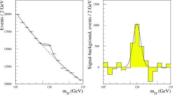
Figure 19: ATLAS simulation of $gg\to H\to\gamma\gamma$ at LHC for $M_{H}=120$ GeV and 30 fb^-1 of data ATLAS_TDR . The right panel is the mass distribution after background subtraction, normalized from sidebands.

II.3.3 Weak boson fusion Higgs production

Let’s explore this other production mechanism I said isn’t accessible at Tevatron, weak boson fusion (WBF). It was long ignored for LHC light Higgs phenomenology because its rate is about an order of magnitude smaller than $gg\to H$ there. However, it has quite distinctive kinemattics and QCD properties that make it easy to suppress backgrounds, for all Higgs decay channels. The process itself is described by an incoming pair of quark partons which brem a pair of weak gauge bosons, which fuse to produce a Higgs; see Fig. 20.

The first distinctive characteristic of WBF is that the quarks scatter with significant transverse momentum, and will show up as far forward and backward jets in the hadronic calorimeters of CMS and ATLAS. The Higgs boson is produced centrally, however, so its decay products, regardless of decay mode, typically show up in the central detector region. This is shown in the lego plot schematic in the right panel of Fig. 20.

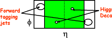
Figure 20: WBF Higgs production Feynman diagram and lego plot schematic of a typical event.

The reason for this scattering behavior comes from the $W$ (or $Z$) propagator, $1/(Q^{2}-M^{2})$. For $t$-channel processes, $Q^{2}$ is necessarily always negative. Thus the propagator suppresses the amplitude least when $Q^{2}$ is small. For small $Q^{2}$, we have $Q^{2}=(p_{f}-p_{i})^{2}\approx E_{q}^{2}(1-x)\theta^{2}$, where $x$ is the fraction of incoming quark energy the weak boson takes with it, and is small. Thus $\theta$ prefers to be small, translating into large pseudorapidity. One quark will be scattered in the far forward detector, the other far backward, and the pseudorapidity separation between them will tend to be large. We call these “tagging” jets. QCD processes with an extra EW object(s) which mimics a Higgs decay, on the other hand, have a fundamentally different propagator structure and prefer larger scattering angles early_WBF-H ; Rainwater:1996ud , including at NLO Campbell:2003hd . The differences between the two are shown in Fig. 21 Asai:2004ws .

The second distinctive characteristic is QCD radiation QCDrad . Additional jet activity in WBF prefers to be forward of the scattered quarks. This is because it occurs via bremsstrahlung off color charge, which is scattered at small angles, with no connection between them. In contrast, QCD production always involves color charge being exchanged between the incoming partons: acceleration through 180 degrees. QCD bremsstrahlung thus takes place over large angles, covering the central region. Central jet activity can be vetoed, giving large background suppression Barger:1994zq . We won’t discuss it further, due to theoretical uncertainties; the interested student may learn more from Ref. Rainwater:1999gg .

Figure 21: Tagging jet rapidity (left) and separation (right) for WBF Higgs production v. QCD $t\bar{t}$ production Asai:2004ws .

We’ll see in the next few subsections that WBF Higgs channels are extremely powerful even without a central jet (minijet) veto. Eventually a veto will be used, after calibration from observing EW v. QCD $Zjj$ production in the early running of LHC Rainwater:1996ud . There is however another lingering theoretical uncertainty, coming from Higgs production itself!

QCD Higgs production via loop-induced couplings may itself give rise to two forward tagging jets, which would then fall into the WBF Higgs sample gg_Hjj . Some representative Feynman diagrams for this process are shown in Fig. 22. After imposing WBF-type kinematic cuts (far forward/backward, well-separated jets, central Higgs decay products), this contribution to the WBF sample adds about another third for a light Higgs, or doubles it for a very heavy Higgs, $M_{H}\gtrsim 350$ GeV, as shown in the left panel of Fig. 23. The residual QCD theoretical cross section uncertainty is about a factor of two, however, and being QCD it will produce far more central jets, which will be vetoed to reject QCD backgrounds. Naïvely, then, gluon fusion $Hjj$ is an $\sim 10\%$ contribution to WBF, but with a huge uncertainty.

This contribution is a mixed blessing. It’s part of the signal, so would hasten discovery. Yet it creates confusion, since at some point we want to measure couplings, and the WBF and gluon fusion components arise from different couplings. Fortunately, there is a difference! WBF produces an almost-flat distribution in $\phi_{jj}$, the azimuthal tagging jet separation, but gluon fusion has a suppression at 90 degrees gg_Hjj ; cf. right panel of Fig. 23.

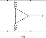
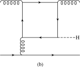
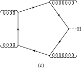
Figure 22: Representative Feynman diagrams for gluon fusion Higgs plus two jets production gg_Hjj .

Figure 23: Left: WBF and gluon fusion contributions to the forward-tagged $Hjj$ sample at LHC. Right: azimuthal angular distributions for the same two processes, showing distinctive differences. Figures taken from Ref. gg_Hjj .

II.3.4 Weak boson fusion $H\to\tau^{+}\tau^{-}$

Now we know that the WBF signature can strongly suppress QCD backgrounds because of its unique kinematic characteristics. We expect that $H\to\gamma\gamma$ is visible in WBF Rainwater:1997dg ; Buscher:2005re ; CMS_TDR , but being a rare decay in a smaller-rate channel, it’s not expected to lead to discovery. Rather, it would be a useful additional channel for couplings measurements. Let’s now instead discuss a decay mode we haven’t yet considered, $H\to\tau^{+}\tau^{-}$. This is sub-dominant to $H\to b\bar{b}$ in the light Higgs region, $M_{H}\lesssim 150$ GeV, but the backgrounds are more EW than QCD. We thus have some hope to see it, whereas $H\to b\bar{b}$ remains frustratingly hopeless.

We first have to realize that taus decay to a variety of final states:

• $35\%$ $\tau\to\ell\nu_{\ell}\nu_{\tau}$, ID efficiency $\epsilon_{\ell}\sim 90\%$

• $50\%$ $\tau\to h_{1}\nu_{\tau}$ “1-prong” hadronic (one charged track), ID efficiency $\epsilon_{h}\sim 25\%$

• $15\%$ $\tau\to h_{3}\nu_{\tau}$ “3-prong” hadronic (three charged tracks), which are thrown away

The obvious problem is that with at least two neutrinos escaping, the Higgs cannot be reconstructed from its decay products. Or can it?

Let’s assume the taus decay collinearly. This is an excellent approximation: since 50+ GeV energy taus have far more energy than their mass, so their decay products are highly collimated. We then have two unknowns, $x_{+}$ and $x_{-}$, the fractions of tau energy that the charged particles take with them. What experiment measures is missing transverse energy in the $x$ and $y$ directions. Two unknowns with two measurements is exactly solvable. For our system this gives Ellis:1987xu :

$$m_{\tau^{+}\tau^{-}}^{2}\;=\;\frac{m_{\ell^{+}\ell^{-}}^{2}}{x_{+}x_{-}}+2m_{\tau}^{2}$$ (11)

(an excellent exercise for all students to get a grip on kinematics and useful tricks at hadron colliders). An important note is that this doesn’t work for back-to-back taus (the derivation will reveal why), but WBF Higgses are typically kicked out with about 100 GeV of $p_{T}$, so this almost never happens in WBF. This trick can’t be used in the bulk of $gg\to H$ events because there it is produced mostly at rest with nearly all taus back-to-back.

We need a lepton trigger, so consider two channels: $\tau^{+}\tau^{-}\to\ell^{\pm}h$ and $\tau^{+}\tau^{-}\to\ell^{+}\ell^{\prime-}$ ($\ell=e,\mu$). The main backgrounds are EW and QCD $Zjj$ production (really $Z/\gamma^{*}$), top quark pairs, EW & QCD $WWjj$ and QCD $b\bar{b}jj$ production. But after reconstruction, the non-$Z$ backgrounds look very different than the signal in $x_{+}$–$x_{-}$ space, as shown in Fig. 24.

ATLAS and CMS have both studied these channels with full detector simulation and WBF kinematic cuts, but no minijet veto, and found extremely promising results Asai:2004ws . Fig. 25 shows invariant mass distributions for a reconstructed Higgs in the two different decay channels, assuming only 30 fb^-1 of data. The Higgs peak is easily seen above the backgrounds and away from the $Z$ pole. Mass resolution is expected to be a few GeV.

Figure 24: Reconstructed $x_{+}$ v. $x_{-}$ ($x_{1}$, $x_{2}$) for a WBF $H\to\tau^{+}\tau^{-}$ signal v. non-$Z$ backgrounds Plehn:1999xi .

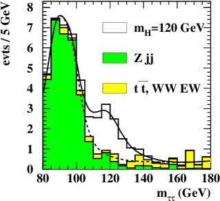
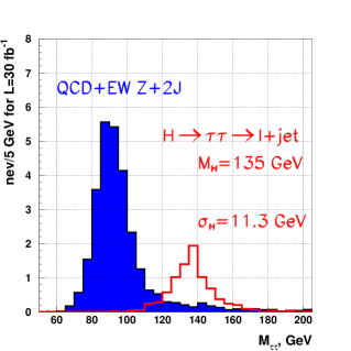
Figure 25: ATLAS (left) and CMS (right) simulations of WBF $H\to\tau^{+}\tau^{-}$ events after 30 fb^-1 of data at LHC. The Higgs resonance clearly stands out from the background. Figures from Ref. Asai:2004ws .

But this joint study by CMS and ATLAS Asai:2004ws is not the best we can do. The joint study ignored the minijet veto, for instance. While that will assuredly improve the situation further, we’re just not sure precisely how much. Putting this aside for the moment, there are yet further tricks to play to improve the situation.

The leading idea zeroes in on the fact that missing transverse momentum ($/\!\!\!p_{T}$) has some uncertainty due to jet energy mismeasurement (those imperfect detectors). Using a $\chi^{2}$ test, one determines which is more likely: $Z\to\tau^{+}\tau^{-}$ or $H\to\tau^{+}\tau^{-}$, using a fixed Higgs mass constraint Cranmer-taus . Examining the schematics in Fig. 26, we see this is tantamount to deciding which fit is closer to the center of the $/\!\!\!p_{T}$ uncertainty region. Early indications are that this technique would improve $S/B$ by about a factor four, in addition to recovering some signal lost using more traditional strict kinematic cuts on $x_{+}$ and $x_{-}$ (recall Fig. 24). This would approximately halve the data required to discover a light SM Higgs boson using this channel. Keep it in mind when we see the current official discovery expectations in Sec. II.3.7. Further improvements might also be expected from neural-net type analyses, which are coming to the fore now that Tevatron has demonstrated their viability.

A final word on systematic uncertainties. Unlike the tortuous case of $t\bar{t}H,H\to b\bar{b}$, we don’t have to worry about shape systematics here. The dominant background is $Zjj$ production. We can separately examine $Z\to ee,\mu\mu$, which produces an extremely sharp, clean peak, precisely calibrating $Zjj$ production in Monte Carlo. The only uncertainty then is tau decay modeling, which is very well understood from the LEP era.

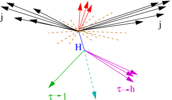
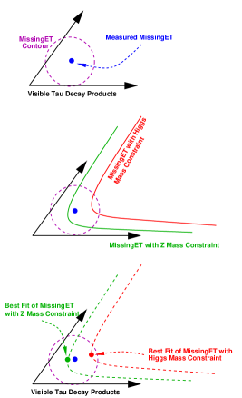
Figure 26: Left: schematic azimuthal projection of WBF $H\to\tau^{+}\tau^{-}$ events at LHC. Right: diagram illustrating the $1\sigma$ uncertainty region (due to jet mismeasurement) of missing $p_{T}$, and how a $Z$ mass or Higgs mass hypothesis can be best fit using a $\chi^{2}$ test. Figures from Ref. Cranmer-taumod .

II.3.5 Weak boson fusion $H\to W^{+}W^{-}$

A natural question to ask is, how well does WBF Higgs hunting work for $M_{H}\gtrsim 140$ GeV, where $H\to W^{+}W^{-}$ dominates? We should expect fairly well, since it’s the production process characteristics that supply most of the background suppression, leaving us only to look for separated reconstructed mass peaks.

For $H\to W^{+}W^{-}$ we’ll consider only the dilepton channel, as it has relatively low backgrounds, while QCD gives a large rate for the other possible channel, one central lepton plus two central jets (and the minijet veto will likely not work). We’ll therefore rely on exactly the same angular correlations and transverse mass variable we encountered in the Tevatron case Rainwater:1999sd (cf. Eqs. 8,9). The only critical distinction is then $e\mu$ v. $ee$, $\mu\mu$ samples, as the latter have a continuum background ($Z^{*}/\gamma^{*}$). These are not too much of a concern, however.

Without going too much into detail, I’ll simply say that top quarks are a major background, and they have the largest uncertainty. The largest component comes from $t\bar{t}j$ production, where the extra hard parton is far forward and ID’d as one tagging jet; a $b$ jet from top decay gives the other tagging jet, and the other $b$ jet is unobserved. This background requires care to simulate, because the soft/collinear approximation in standard codes is no good. There is also a significant contribution from single-top production, and off-shell effects are crucial to simulate, which is not normally an issue for backgrounds at LHC OFS-tops . Work is still needed in this area to be fully prepared for this particular search channel. Fortunately, we may expect an NLO calculation of $t\bar{t}j$ before LHC start DUW .

Fig. 27 shows the results of the same ATLAS/CMS joint WBF Higgs study for this channel Asai:2004ws . The results are extremely positive, with $S/B>1/1$ without a minijet veto over a large mass range; even for $M_{H}=120$ GeV, $S/B\sim 1/2$, allowing for Higgs observation even down to the LEP limit in this channel. The transverse mass variable works extremely well for Higgs masses near $WW$ threshold, and reasonably well for lower masses, where the $W$ bosons are off-shell.

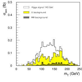
Figure 27: ATLAS simulations of WBF $H\to W^{+}W^{-}$ events after 30 fb^-1 of data at LHC for $M_{H}=140$ GeV (left) and 160 GeV (right). The Higgs signal clearly stands out from the background in both cases, although the Jacobian peak is easier to identify closer to threshold. Figures taken from Ref. Asai:2004ws .

II.3.6 $t\bar{t}H,H\to W^{+}W^{-}$ at higher mass

A late entry to the Higgs game at LHC is top quark associated production, but with Higgs decaying to $W$ bosons. Representative Feynman diagrams are shown in Fig. 28. Obviously this is intended to apply to larger Higgs masses, but turns out to work fairly well even below $W$ pair threshold Maltoni:2002jr ; ATL-PHYS-2002-019 . The key is to use same-sign dilepton and trilepton subsamples. The backgrounds then don’t come from pure QCD production, rather from mixed QCD-EW top quark pairs plus $W$, $Z/\gamma^{*}$, $W^{+}W^{-}$, etc. We would be especially eager to observe this channel because, if the $HWW$ coupling is measured elsewhere, it provides the only viable direct measurement of the top quark Yukawa coupling. More on this in Chapter III.

A noteworthy features of this channel is that while the $t\bar{t}H$ cross section falls with increasing $M_{H}$, BR($H\to W^{+}W^{-}$) rises with increasing $M_{H}$ in our mass region of interest, and the two trends coincidentally approximately balance each other. From a final-state rate perspective, this channel is approximately constant over a wide mass range, up to about 200 GeV. Fig. 29 shows this numerically. Fig. 30 shows ATLAS’s expected statistical uncertainty on the top quark Yukawa coupling. It ranges from about $20\%$ over a broad mass range for 30 fb^-1 of data, to about $10\%$ from the full LHC run. Systematic uncertainties are currently unexplored.

Figure 28: Representative Feynman diagrams for $t\bar{t}H,H\to W^{+}W^{-}$ production at LHC.

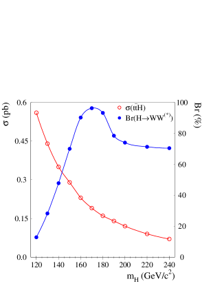
Figure 29: Left: $t\bar{t}H$ cross section and BR($H\to W^{+}W^{-}$) as a function of $M_{H}$. Right: the cross section to three different final states after top quark and Higgs decays. Figures from Ref. ATL-PHYS-2002-019 .

Figure 30: ATLAS prediction ATL-PHYS-2002-019 for the top quark Yukawa coupling measurement uncertainty (statistical only) from $t\bar{t}H,H\to W^{+}W^{-}$, for separate leptonic final-state channels and combined.

II.3.7 LHC Higgs in a nutshell

LHC Higgs phenomenology has come a long way in the decade since the first comprehensive studies were reported (e.g. the ATLAS TDR ATLAS_TDR ). The old studies give a seriously misleading picture of LHC capabilities. Students should refer to newer ATLAS Notes and the new CMS TDR CMS_TDR . Solid grounds exist for expecting even more improvements. Fig. 31 summarizes ATLAS’s projections for multiple Higgs channels as a function of Higgs mass. Note especially the new dominance of WBF channels and degradation of $t\bar{t}H$.

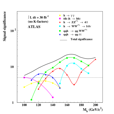
Figure 31: ATLAS significance projections in multiple Higgs channels w/ 30 fb^-1 of LHC data Asai:2004ws .

III Is it the Standard Model Higgs?

Imagine yourself in 2010 (hey, we’re optimists!), squished shoulder-to-shoulder in the CERN auditorium, waiting for the speaker to get to the punchline. Rumors have been circulating for months about excess events showing up in some light Higgs channels, but not all that would be expected. LHC has 40 fb^-1, after all. Your experimental friends tell you that both collaborations have been scrambling madly, independent groups cross-checking the original first analyses. Then the null result slides start passing by. No diphoton peaks anywhere. Nothing in the $WW$ or $ZZ$ channels. Even CMS’s invisible Higgs search (WBF – tagging jets with no central objects at all) doesn’t show anything. Numerous standard MSSM Higgs results fly by, invariant mass spectra fitting the SM predictions perfectly. The audience becomes restless, irritated. People around you mutter that there must not be a Higgs after all. But you realize that the speaker skipped mention of the WBF $H\to\tau^{+}\tau^{-}$ channel. Then suddenly it appears, and there’s a peak above the $Z$ pole, centered around 125 GeV, broader than you’d expect but the speaker says something about resolution will improve with further refinement of the tau reconstruction algorithms. It’s also a too-small rate, less than half what’s expected.

So what is this beast? The bump showed up in a Higgs search channel, but at that mass it should have shown up in several others as well. If it’s Standard Model, that is. At 125 GeV there should be $H\to W^{+}W^{-}$ in WBF, and $H\to\gamma\gamma$ both inclusively and in WBF, although maybe they’re still marginal. Photons turned out to be hard at first, and QCD predictions weren’t quite on the mark. Quite a few people are on their cell phones already. You hear a dozen different exclamations, ranging from “We found the Higgs!” to “The Standard Model is dead!”. Quite obviously this is a new physics discovery, but what exactly is going on?

By now you should get the point of this imaginary scenario: finding a new bump is merely the start of real physics. For numerous reasons you’ve heard at this summer school, some better than others, finding a SM Higgs really isn’t very likely. But as we’ll see in Chapter IV, SM Higgs phenomenology is a superb base for beyond-the-SM (BSM) Higgs sectors. They’re variations on a theme in some sense, with the occasional special channel thrown in, like the invisible Higgs search alluded to above. Our job will be to figure out what any new resonance is. But how do we go about doing that in a systematic way that’s useful to theorists for constructing the New Standard Model?

For starters, we want to know the complete set of quantum numbers for any Higgs candidate we find. Standard Model expectations will probably prejudice us as to what they are (roughly, at least) based on which search channel a bump shows up in. But for the scenario above, I can envision at least three very reasonable yet completely different models that would give that kind of a result in early LHC running. We should keep in mind that further data may reveal more resonances – not everything is easy to see against backgrounds, or is produced with enough rate to emerge with only 1/10 of the planned LHC data. In some cases we would have to wait much longer, using data from the planned LHC luminosity upgrade (SLHC) Gianotti:2002xx . New physics could also mean new quantum numbers that we don’t yet know about, so we should be prepared to expand our list of measurements needed to sort out the theory, and spend time now thinking about what kinds of observables are even possible at the LHC. Some measurements will almost certainly require the clean environment of a future high-energy electron-positron machine like an ILC Aguilar-Saavedra:2001rg ; Gunion:2003fd . The most complete picture would emerge only after combining results Weiglein:2004hn , which could take than a decade. In the meantime we might get a good picture of the new physics, but not its details.

Let’s prepare a preliminary list of quantum numbers we need to measure for a candidate Higgs resonance, which I’ll generically call $\phi$. In brackets is the SM expectation. I’ll order them in increasing level of difficulty. (See also the review article of Ref. Burgess:1999ha .)

• electric charge [neutral]

• color charge [neutral]

• mass [free parameter]

• spin [0]

• CP [even]

• gauge coupling ($g_{WWH}$) [$SU(2)_{L}$ with tensor structure $g^{\mu\nu}$]

• Yukawa couplings [$m_{f}/v$]

• spontaneous symmetry breaking potential (self-couplings) [fixed by the mass]

Of course, the first two of those, electric and color charge, are known immediately from the decay products. (A non-color-singlet scalar is a radically different beast than the SM Higgs and would have dramatically different couplings and signatures.) Mass is also almost immediate, with some level of uncertainty that depends almost purely on detector effects. Spin and CP are related to some degree, and not entirely straightforward if the Higgs sector is non-minimal and contains CP violation. Gauge and Yukawa couplings are generally regarded as the most crucial observables, and in some sense I would agree. However, I would argue that the linchpin of spontaneous symmetry breaking (SSB) is the existence of a Higgs potential, which requires Higgs self-couplings. Measuring these and finding they match to some gauge theory with a SSB Higgs sector would to me be the most definitive proof of SSB, and strongly suggest that the Higgs is a fundamental scalar, not composite. It is also the most difficult task – perhaps not even possible.

A cautionary note: the results I show in this section are in general applicable only to the Standard Model Higgs! This point is often lost in many presentations highlighting the capabilities of various experiments, but it is very easy to understand. For example, if for some reason the Higgs sector has suppressed couplings to colored fermions, then any measurement of, say, the $b$ Yukawa coupling, will be less precise, simply because the signal rate is lower, yet the background remains fixed. It’s statistics!

III.1 Mass measurement

As already noted, our Higgs hunt pretty much gets us this quantum number immediately, but with some slop driven by detector performance. We want to measure it as accurately as possible, but in practice a GeV or so is good enough, because theoretical uncertainties in parameter fits tend to dominate for most BSM physics. (This is a long-standing problem in SUSY scenarios, for example. It may be that we need to know the Higgs mass theoretical prediction to four loops Spira ; at present only a partial three-loop calculation is known Martin:2007pg , and only two-loop results exist in usable code Hahn:2006np .) Fig. 32 shows the CMS and ILC expected Higgs mass precision as a function of $M_{H}$ Drollinger:2001bc . It varies, of course, because different decay modes are accessible at different $M_{H}$, and detector resolution depends on the final state. In general, photon pairs ($H\to\gamma\gamma$) and four leptons coming from $Z$ pairs ($H\to ZZ\to\ell^{+}\ell^{-}\ell^{\prime+}\ell^{\prime-}$) will give the most precise measurement. As a rule of thumb, we may expect per-mille precision over a broad mass range, translating typically to a few hundred MeV.

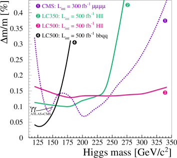
Figure 32: Expected SM Higgs mass precision at LHC (for CMS; ATLAS will be slightly different but comparable) and a future ILC, as a function of Higgs mass Drollinger:2001bc .

III.2 Spin & CP measurement

Spin and CP ($J^{PC}$) experimental measurements are linked, because both require angular distributions to obtain. Numerous techniques have been proposed to address this, with significant overlap but also some unique features with each method. I’ll highlight the leading proposals which garner the most attention from LHC experimentalists today.

From the observed final state we can tell that the Higgs candidate is a boson. We’ll start by assuming that it may be spin 0, 1 or 2, but no higher. Then we recall that the Yang-Landau Theorem Yang:1950rg forbids a coupling between three $S=1$ bosons if two of them are identical. Thus, if we observe $\phi\to\gamma\gamma$, then our new object cannot be spin-1, and $C=1$. For the very curious student who wants to delve deeper, there is a recent report on CP Higgs studies at colliders Accomando:2006ga .

III.2.1 Nelson technique

The first method is the oldest, developed by Nelson Dell'Aquila:1985vc . It assumes the object is a scalar or pseudoscalar and relies on the decay angular distributions to a pair of EW gauge bosons, which decay further. The most practical aspect relevant for LHC Higgs physics is in essence a measurement of the relative azimuthal angle between the decay planes of two $Z$ bosons in turn coming from the scalar decay, in the scalar particle’s rest frame. See Fig. 33 for clarity. One bins the data in this distribution and fits to the equation:

$$F(\phi)\,=\,1+\alpha\cos(\phi)+\beta\cos(2\phi)$$ (12)

For a scalar, such as the SM Higgs, the coefficients $\alpha$ and $\beta$ are functions of the scalar mass, and further we have the constraint that $\alpha(M_{\phi})>\frac{1}{4}$. In contrast, for a pseudoscalar, $\alpha=0$ and $\beta=-0.25$, independent of the mass.

Ref. Buszello:2002uu was the first to apply this to the LHC Higgs physics program using detector simulation. Assuming 100 fb^-1 of data, the study found that LHC could readily distinguish a SM Higgs from a pseudoscalar for $M_{H}>200$ GeV, and from a spin-1 boson of either CP state from a little above that, but not right at 200 GeV; see Fig. 34. Applying this technique to $M_{H}<200$ but above $ZZ$ threshold was not examined.

As a practical matter, $H\to ZZ^{(*)}$ observation is assured only for both $Z$ bosons decaying to leptons ($e$ or $\mu$), where there is essentially zero background. Unfortunately, this is an extremely tiny branching ratio, only $0.05\%$ of all $H\to ZZ$ events. Some studies consider $jj\ell^{+}\ell^{-}$ channels, which is a ten-times larger sample, in an attempt to increase statistics, but this suffers from non-trivial QCD backgrounds.

Figure 33: Schematic of the azimuthal angle between the decay planes of $Z$ bosons arising from massive scalar decay. All angles are in the scalar rest frame. Figure from Ref. Buszello:2002uu .

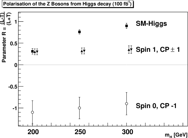
Figure 34: Results of the LHC expectations spin/CP study of Ref. Buszello:2002uu , showing how a SM Higgs could be distinguished from a pseudoscalar or spin-1 boson as a function of $M_{H}$.

III.2.2 CMMZ technique

Ref. Choi:2002jk provides an extension to the Nelson technique below $ZZ$ threshold. Its full analysis is far more in-depth, discussing the angular behavior of the matrix elements for arbitrary boson spin and parity. It first demonstrates how objects of odd normality (spin times parity) can be discriminated via angular distributions, but for even normality require a further discriminant. That is, a $J^{P}=2^{+}$ boson could mimic a SM Higgs in angular distribution below $ZZ$ threshold. (Exotic higher spin states can be trivially ruled out via the lack of angular correlation between the beam and the object’s flight direction.)

The key discriminant is the differential partial decay rate for the off-shell $Z$ boson. It depends on the invariant mass of the final-state lepton pair and is linear in $Z^{*}$ velocity:

$$\frac{d\Gamma_{H}}{dM_{*}^{2}}\;\sim\;\beta\;\sim\;\sqrt{(M_{H}-M_{Z})^{2}-M_{*}^{2}}$$ (13)

Fig. 35 shows the predicted distributions for 150 GeV spin-0,1,2 even-normality objects as a function of $M_{*}$, the off-shellness of the $Z^{*}\ell^{+}\ell^{-}$. The histogram represents about 200 events that a SM Higgs would give in this channel after 300 fb^-1 of data at LHC. Unfortunately there are no error bars, although one can estimate the statistical uncertainty for each bin as $\sqrt{N}$ and observe that the measurement is likely not spectacular. We can expect that CMS and ATLAS will eventually get around to quantifying the discriminating power, but it would not be surprising to learn that this measurement requires far more data, e.g. at the upgraded SLHC Gianotti:2002xx .

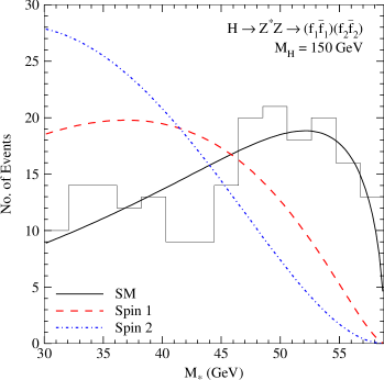
Figure 35: Differential decay rate as a function of dilepton invariant mass of the off-shell $Z^{*}$ in $ZZ$ events, for a 150 GeV SM Higgs v. spin-1 and spin-2 objects of even normality and the same mass. The histogram is the SM Higgs case for 300 fb^-1 of data at LHC. Figure from Ref. Choi:2002jk .

III.2.3 CP and gauge vertex structure via WBF

A third technique Plehn:2001nj takes a different approach, but addressing spin and CP in a slightly different way. Rather than examine Higgs decays, it notes that WBF Higgs production is observable for any Higgs mass, regardless of decay mode. Furthermore, the same $HVV$ vertex appears on the production side for all masses, also independent of decay. More precisely, this vertex has the structure $g^{\mu\nu}HV_{\mu}V_{\nu}$ ($V=W,Z$). This tensor structure is not gauge invariant by itself. It must come from a gauge-invariant kinetic term $(D_{\mu}\Phi)^{\dagger}(D^{\mu}\Phi)$. Identifying it in experiment would go a long way to establishing that the scalar field is a remnant of spontaneous symmetry breaking.

For a scalar field which couples via higher-dimensional operators to two gauge bosons, however, we may write down the CP-even and CP-odd gauge-invariant D6 operators Buchmuller:1985jz :

$${\cal L}_{6}\;=\;\frac{g^{2}}{2\Lambda_{6,e}}(\Phi^{\dagger}\Phi)W^{+}_{\mu\nu}W^{-\mu\nu}\;+\;\frac{g^{2}}{2\Lambda_{6,o}}(\Phi^{\dagger}\Phi)\widetilde{W}^{+}_{\mu\nu}W^{-\mu\nu}$$ (14)

where $\Lambda_{6}$ is the scale of new physics that is integrated out, $W^{\mu\nu}$ is the $W$ boson field strength tensor, and $\widetilde{W}=\epsilon_{\alpha\beta\mu\nu}W^{\alpha\beta}$ is its dual. After expanding $\Phi$ with a vev and radial excitation, we obtain two D5 operators:

$${\cal L}_{5}\;=\;\frac{1}{\Lambda_{5,e}}HW^{+}_{\mu\nu}W^{-\mu\nu}\;+\;\frac{1}{\Lambda_{5,o}}H\widetilde{W}^{+}_{\mu\nu}W^{-\mu\nu}$$ (15)

where $\Lambda_{5}$ are dimensionful but now parameterize both the D6 coefficients and the $\Phi$ vev.

These two D5 operators produce very distinctive matrix element behavior. Recalling that the external gauge bosons in WBF are actually virtual and connect to external fermion currents, the initial-state scattered quarks, we derive the following approximate relations for the CP-even operator, using $J_{1,2}$ for the incoming fermion currents:

$${\cal M}_{e,5}\propto\frac{1}{\Lambda_{e,5}}J^{\mu}_{1}J^{\nu}_{2}\biggl{[}g_{\mu\nu}(q_{1}\cdot q_{2})-q_{1,\nu}q_{2,\mu}\biggr{]}\sim\frac{1}{\Lambda_{e,5}}[J^{0}_{1}J^{0}_{2}-J^{3}_{1}J^{3}_{2}]\;\vec{p}_{T}^{\;j1}\cdot\vec{p}_{T}^{\;j2}$$ (16)

That is, the amplitude is proportional to the tagging jets’ transverse momentum dot product. This is easy to measure experimentally – we just plot the azimuthal angular distribution, i.e. angular separation in the plane perpendicular to the beam. It will be minimal, nearly zero, for $\phi_{jj}=\pi/4$. In contrast, the $g^{\mu\nu}$ tensor structure of the SM Higgs mechanism does not correlate the tagging jets. The CP-odd D5 operator is different and more complex, but may be understood by noting that it contains a Levi-Civita tensor $\epsilon^{\mu\nu\rho\delta}$ connecting the external fermion momenta. This is non-zero only when the four external momenta are independent, i.e. not coplanar. Thus this distribution will be zero for $\phi_{jj}=0,\pi$.

Fig. 36 shows the results of a parton-level simulation for scalars in both the mass range where decays to taus would be used, and where $\phi\to W^{+}W^{-}$ dominates. The SM signal curve is not entirely flat due to kinematic cuts imposed on the final state to ID all objects. The D5 operators produce behavior qualitatively distinct from spontaneous symmetry breaking, with minima for the distributions exactly where expected, and orthogonal from each other. It would be essentially trivial to distinguish the cases from each other shortly after discovery, regardless of $M_{H}$ and the particular channel used to discover the Higgs candidate. A key requirement for this, of course, is that the discovery searches don’t use this distribution to separate signal from background.

Figure 36: Azimuthal angular distributions of the tagging jets in WBF production of a SM Higgs v. scalar field coupled to weak bosons via CP-even/odd D6 operators. The dotted line in the left panel is the SM background, which is added to the signal curves. Figures from Ref. Plehn:2001nj .

Now, what happens if the Higgs indeed arises from SSB, but new physics generates sizable D6 operators? Since $H_{\rm SM}$ is CP-even, a CP-even D5 operator would interfere with the SM amplitude, while a CP-odd contribution would remain independent. This is illustrated in the left panel of Fig. 37. The obvious thing to do is create an asymmetry observable sensitive to this interference:

$$A_{\phi}\;=\;\frac{\sigma(\Delta\phi_{jj}<\pi/2)-\sigma(\Delta\phi_{jj}>\pi/2)}{\sigma(\Delta\phi_{jj}<\pi/2)+\sigma(\Delta\phi_{jj}>\pi/2)}$$ (17)

With only 100 fb^-1 of data at LHC (one experiment), this asymmetry would have access to $\Lambda_{6}\sim 1$ TeV, which is itself within the reach of LHC, likely resulting in new physics observation directly. One caveat: the study Ref. Plehn:2001nj was done before the $gg\to Hgg$ contamination gg_Hjj was known, which will complicate this measurement.

Figure 37: Left: As in Fig. 36, but with interference between the SM Higgs and a CP-even D5 operator. Right: the effective reach in $\Lambda_{5,e}$ for 100 fb^-1 at LHC, using only the rate information (top) or the asymmetry (bottom). Figures from Ref. Plehn:2001nj .

III.2.4 Spin and CP at an ILC

The much cleaner, low-background environment of $e^{+}e^{-}$ collisions would be an excellent environment to study a new resonance’s spin and CP properties. $J^{PC}$ can in fact be determined completely model-independently. Recalling the LEP search, the canonical production mechanism is $e^{+}e^{-}\to ZH$. We would identify the $Z$ via its decay to leptons, and sum over all Higgs decays (this is possible using the recoil mass technique, coming up in Sec. III.4). $J$ and $P$ are completely determined by a combination of the cross section rise at threshold and the polar angle of the $Z$ flight direction in the lab, shown in the left panel of Fig. 38. The differential cross section is Aguilar-Saavedra:2001rg :

$$\frac{d\sigma}{d\cos\theta_{Z}}\propto\beta\bigl{[}1+a\beta^{2}\sin^{2}\theta_{Z}+b\eta\beta\cos\theta_{Z}+\eta^{2}\beta^{2}(1+\cos^{2}\theta_{Z})\bigr{]}$$ (18)

where $a$ and $b$ depend on the EW couplings and $Z$ boson mass, $\eta$ is a general pseudoscalar (loop-induced) coupling and $\beta$ is the velocity. Far more sophisticated analyses techniques exist, often called “optimal observable” analyses Hagiwara:2000tk , but are only for the terminally curious.

If one would have the liberty to perform a threshold scan of $Z\phi$ production at an ILC, distinguishing given-normality $J=0,1,2$ states is straightforward due to their different $\beta$-dependence. For $J=0$ it is linear, but for higher spin is higher-power in $\beta$ Miller:2001bi . The qualitative behavior is shown in the right panel of Fig. 38, complete with error bars for the SM Higgs case. However, while the physics is solid, experiments in the past have generally proved to be a horse race for highest energy, so there is no guarantee that one would have threshold scan data available. The angular distribution fortunately works at all energies.

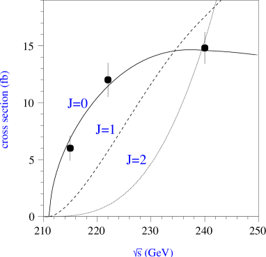
Figure 38: Left: Feynman diagram for $e^{+}e^{-}\to ZH$ and schematic Miller:2001bi showing the analyzing angles. Right: curves showing the threshold rate dependence for $J=0,1,2$ states in this channel Aguilar-Saavedra:2001rg .

III.3 Higgs couplings at LHC

Now to something much harder. It’s commonly believed that LHC cannot measure Higgs couplings, only ratios of BRs ATLAS_TDR . This is incorrect, but requires a little explanation to understand why people previously believed in a limitation.

First, let me state that the LHC doesn’t measure couplings or any other quantum number directly. It measures rates. (This is true for any particle physics experiment.) From those we extract various $\sigma_{i}\cdot{\rm BR}_{j}$ by removing detector, soft QCD and phase space effects, among other things, using Monte Carlo simulations based on known physics inputs.

Second, we note that for a light Higgs, which has a very small width (cf. Sec. II.1.1), the Higgs production cross section is proportional to the partial width for Higgs decay to the initial state (the Narrow Width Approximation, NWA). That is, $\sigma_{gg\to H}\propto\Gamma_{H\to gg}$. Similarly, $\sigma_{\rm WBF}\propto\Gamma_{H\to W^{+}W^{-}}$. The student who has never seen this may easily derive it by recalling the definition of cross section and partial decay width – they share the same matrix elements and differ only by phase space factors. Typically we abbreviate these partial widths with a subscript identifying the final state particle, thus we have $\Gamma_{g}$, $\Gamma_{\gamma}$, $\Gamma_{b}$, etc. Since a BR is just the partial decay width over the total width, we then write:

$$\bigl{(}\sigma_{H}\cdot{\rm BR}\bigr{)}_{i}\propto\biggl{(}\frac{\Gamma_{p}\Gamma_{d}}{\Gamma_{H}}\biggr{)}_{i}$$ (19)

where $\Gamma_{p}$ and $\Gamma_{d}$ are the “production” and decay widths, respectively.

Third, count up the number of observables we have and measurements we can make. Assuming we have a decay channel for each possible Higgs decay (which we don’t), we’re still one short: $\Gamma_{H}$, the total width. Now, if the width is large enough, larger than detector resolution, we can measure it directly. Fig. 39 shows that this can happen only for $M_{H}\gtrsim 230$ GeV or so ATLAS_TDR , far above where EW precision data suggests we’ll find the (SM) Higgs. Below this mass range, we have to think of something else.

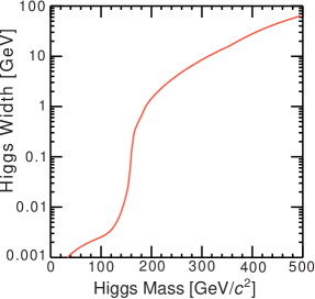
Figure 39: Left: Standard Model Higgs total width as a function of $M_{H}$. Right: expected experimental precision on $\Gamma_{H}$ at ATLAS using the $gg\to H\to ZZ\to 4\ell$ channel ATLAS_TDR (CMS similar).

In the SM, we know precisely what $\Gamma_{H}$ is: the sum of all the partial widths. For the moment let’s assume we have access to all possible decays or partial widths via production, ignore the super-rare decay modes to first- and second-generation fermions. This is a mild assumption, because if for some reason the muon or electron Yukawa were anywhere close to that of taus, where it might contribute to the total width, it would immediately be observable. The list of possible measurements we can form from accessible $(\sigma\cdot{\rm BR})_{i,exp}$ is:

$$X_{\gamma},X_{\tau},X_{W},X_{Z},Y_{\gamma},Y_{W},Y_{Z},Z_{b},Z_{\gamma},Z_{W}$$ (20)

where $X_{i}$ correspond to WBF channels, $Y_{i}$ are inclusive Higgs production, and $Z_{i}$ are top quark associated production. We could easily add measurements like $X_{\mu}$, $Y_{e}$, etc. if we wanted, because measuring zero for any observable is still a measurement – it simply places a constraint on that combination of partial widths or couplings.

In the original implementation of this idea Zeppenfeld:2000td , the authors noted that the $t\bar{t}H,H\to b\bar{b}$ channel won’t work, so there is no access at LHC to $\Gamma_{b}$. However, there is access to $\Gamma_{\tau}$. In the SM, the $b$ and $\tau$ Yukawa couplings are related by $r_{b}=\Gamma_{b}/\Gamma_{\tau}=3c_{\rm QCD}m_{b}^{2}/m_{\tau}^{2}$, where $c_{\rm QCD}$ contains QCD higher-order corrections and phase space effects. $\Gamma_{W}$ and $\Gamma_{Z}$ are furthermore related by $SU(2)_{L}$, although we don’t need to use it. Now write down the derived quantity

$$\widetilde{\Gamma}_{W}\;=\;X_{\tau}(1+r_{b})+X_{W}+X_{Z}+X_{\gamma}+\widetilde{X}_{g}\;=\;\biggl{(}\sum\Gamma_{i}\biggr{)}\frac{\Gamma_{W}}{\Gamma_{H}}\;=\;(1-\epsilon)\Gamma_{W}$$ (21)

where $\widetilde{X}_{g}$ is constructed from $X_{W}$, $X_{\gamma}$, $Y_{W}$ and $Y_{\gamma}$. Although $\Gamma_{\gamma}$ is an infinitesimal contribution to $\Gamma_{H}$, it is important as above, and it contains both the top quark Yukawa and $W$ gauge-Higgs couplings. Our error is contained in $\epsilon$ and is typically small. This provides a good lower bound on $\Gamma_{W}$ from data. The total width is then

$$\Gamma_{H}\;=\;\frac{\widetilde{\Gamma}_{W}^{2}}{X_{W}}$$ (22)

and the error goes as $(1-\epsilon)^{-2}$. Assuming systematic uncertainties of $5\%$ on WBF and $20\%$ on inclusive production, this would achieve about a $10\%$ measurement of $\Gamma_{W}$ and $10-20\%$ on the total width for $M_{H}<200$ GeV.

Voilà! We have circumvented the naïve problem of not enough independent measurements. The astute observer should immediately protest, however, and rightly so. The result is achieved with a little too much confidence that the SM is correct. Not only does the trick rely on a very strong assumption about the $b$ Yukawa coupling, but there could be funny business in the up-quark sector, giving a large partial width to e.g. charm quarks, which would not be observable either via production (too little initial-state charm, and anyhow unidentifiable) or decay (charm can’t be efficiently tagged). Nevertheless, this was a useful exercise, because a much more rigorous, model-independent method is closely based on it.

The more sophisticated method is a powerful least-likelihood fit to data using a more accurate relation than Eq. 19 between data and theory Duhrssen:2004cv :

$$\sigma_{H}\cdot{\rm BR}(H\to xx)\;=\;\frac{\sigma^{\rm SM}_{H}}{\Gamma^{\rm SM}_{p}}\cdot\framebox{$\frac{\Gamma_{p}\Gamma_{d}}{\Gamma_{H}}$}$$ (23)

where the partial widths in the box are the true values to be extracted from data, and the $(\sigma/\Gamma)_{\rm SM}$ ratio in front quantifies all effects shoved into Monte Carlo using SM values: phase space, QCD corrections, detector, etc. As before, the “sum” of all channels provides a solid lower bound on $\Gamma_{H}$, simply because some rate in each of a number of channels requires some minimum coupling. But these are found by a fit, rather than theory assumptions. It also properly takes into account all theory and experimental systematic and statistical uncertainties assigned to each channel. We then need only a firm upper bound on $\Gamma_{H}$ and the fit then extracts absolute couplings (transformed from the partial widths). This bound comes from unitarity: the gauge-Higgs coupling can be depressed via mixing in any multi-doublet model, as well as any number of additional singlets, but it cannot exceed the SM value, which is strictly defined by unitarity. Thus $\Gamma_{V}\leq\Gamma_{V}^{\rm SM}$. (This bound is invalid in triplet models, but these have other characteristics which should make themselves apparent in experiment.) The WBF $H\to W^{+}W^{-}$ channel then provides an upper limit on $\Gamma_{H}$ via its measurement of $\Gamma_{V}^{2}/\Gamma_{H}$.

The method can be further armored against BSM alterations by including the invisible Higgs channel, allowing additional loop contributions, and so on. Of course, the more possible deviations one allows, the larger the fit uncertainties become. We see this in the differences between the left and right panels of Fig. 40 Duhrssen:2004cv . It is obvious that LHC’s weakness is lack of access to $H\to b\bar{b}$. Nevertheless, LHC can measure absolute Higgs couplings with useful constraints on BSM physics. This is especially true for $M_{H}\gtrsim 150$ GeV, where LHC can achieve ${\cal O}(10\%)$ precision on the gauge-Higgs couplings and the total width.

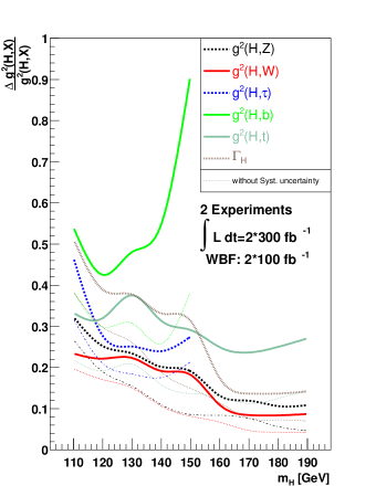
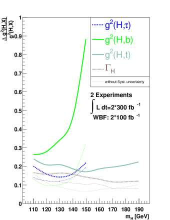
Figure 40: Left: a least likelihood general fit on simulated LHC data, with no additional assumptions about the Higgs sector. Right: the fit assuming no new particles appear in Higgs loop-induced decays, and the gauge-Higgs coupling fixed exactly to the SM value. Figures from Ref. Duhrssen:2004cv .

The fit as implemented in Ref. Duhrssen:2004cv fixes $M_{H}$. This is a slight cheat, since for some $M_{H}$ the BRs change quite rapidly, and a 1-2 GeV uncertainty can lead to a lot of slop in the coupling extraction. This is especially critical for the Higgs sector of the Minimal Supersymmetric Standard Model (MSSM). Eventually a fit to $M_{H}$ will also have to be included, which will degrade measurement precision somewhat.

At the same time, there is cause for optimism. The results of Fig. 40 were based on very conservative, almost pessimistic assumptions: overly-large systematic errors, WBF not being possible at all at high-luminosity running, no minijet veto for WBF (cf. Sec. II.3.3), and lack of progress in higher-order QCD calculations for signals and backgrounds. The reality is that significant progress has been made regarding QCD corrections, and we’ll see one example shortly. Also, everyone knows that the minijet veto is a qualitatively correct aspect of the physics, we just can’t accurately predict its impact. Early LHC data from $Zjj$ production should take care of this. Furthermore, ATLAS and CMS experimentalists fully expect WBF to work at high-luminosity LHC running, they just don’t have full simulation results for the probable efficiencies. Also, we may expect far better performance in the WBF $H\to\tau^{+}\tau^{-}$ channels as discussed in Sec. II.3.4. Finally, if new physics exists up to a few TeV, it will be observable and we can take it into accounts in Higgs loop-induced decays.

Now to QCD corrections. Ref. Duhrssen:2004cv used large QCD uncertainties for $\sigma_{gg\to H}$ and $\Gamma_{g}$, $20\%$ each, which is the correct NNLO uncertainty for each by itself. However, these two quantities appear as a ratio in our observables formula, Eq. 23. As pointed out in Ref. Anastasiou:2005pd , most of these uncertainties drop out in the ratio. The reason for this is that the QCD corrections to the cross section and partial width are largely the same:

$$\Gamma\sim\alpha^{2}_{s}(\mu_{R})C_{1}^{2}(\mu_{R})[1+\alpha_{s}(\mu_{R})X_{1}+...]$$ (24)

$$\sigma\sim\alpha^{2}_{s}(\mu_{R})C_{1}^{2}(\mu_{R})[1+\alpha_{s}(\mu_{R})Y_{1}+...]$$ (25)

The correct uncertainty on the ratio is $5\%$, which will have an enormous impact on the fits of Fig. 40. We eagerly await new results from this and other improvements!

III.4 Higgs couplings at an ILC

Measuring Higgs couplings at an $e^{+}e^{-}$ collider would be far more straightforward and rely on far fewer theoretical assumptions. Between that and being a colorless collision environment, it would also involve far fewer systematic uncertainties. I’ll outline the basic idea.

In fixed-beam collisions it’s possible to measure the total $ZH$ production rate. To see this, we just apply a little relativistic kinematics, rewriting the invariant $M_{H}^{2}$:

$$M^{2}_{H}=p^{2}_{H}=(p_{+}+p_{-}-p_{Z})^{2}=s+M^{2}_{Z}-2E_{Z}\sqrt{s}$$ (26)

We see that observing the Higgs and measuring its total rate boils down to observing $Z$ bosons via their extremely sharp dimuon peak and plotting this recoil mass. Fig. 41 shows what the resulting event rate looks like in this distribution. The Higgs peak is clearly visible and sidebands allow one to subtract the SM background in the signal region. This captures all possible Higgs decays, even though that aren’t taggable or even identifiable, simply by ignoring everything in the event except for the $Z$ dimuons.

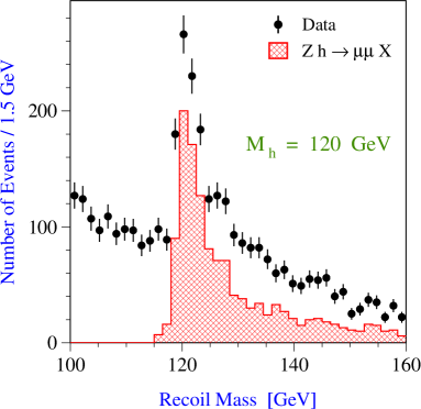
Figure 41: Event rate of the recoil mass for $e^{+}e^{-}\to\mu^{+}\mu^{-}+X$ at a future high-energy linear collider. $ZH$ production will fall into this sample, but the Higgs decays are ignored, thus capturing the total Higgs production rate. (Figure modified from Ref. Garcia-Abia:2000bk for a public talk by one of the authors.)

Simulations Aguilar-Saavedra:2001rg suggest that the recoil mass technique would allow for about a $2.5\%$ absolute measurement of the $ZH$ rate. Since the cross section depends on the $Z$–Higgs coupling squared, the coupling uncertainty is then about a percent.

Getting from this one coupling and the total rate to any other coupling is formulaic:

• In the total rate, measure the best branching ratios, whatever they may be. Depending on the mass and detector performance, that’s likely one of $b\bar{b}$, $\gamma\gamma$ or $W^{+}W^{-}$ decays.

• Now look in WBF Higgs production with the Higgs decaying to the same best final state. This yields the partial width $\Gamma_{W}$.

• Calculate the total Higgs width as $\Gamma_{W}/BR(H\to W^{+}W^{-})$.

• Any other measured BR now gives that individual partial width, therefore the relevant coupling (or couplings for some loop-induced decays).

Table 2 enumerates the results of ILC simulation for select $M_{H}$ Abe:2001np . (Clearly more thorough work should be done here.) There are a few noteworthy features. First, $H\to b\bar{b}$ would be accessible even as a rare BR at larger $M_{H}$, due to the nearly QCD-free collision environment. Second, a weak measurement of $H\to c\bar{c}$ should be possible, for the same reason, and due to the superior $b$ v. $c$ resolution of the next generation of collider detectors. Third, $H\to jj$ is also accessible. This would be attributed to $gg$, which is a mild theoretical assumption. It is in principle sanity-checkable by the absence of an anomalous high-$x$ Higgs production rate at LHC, which would come from sea or valence quarks and a non-SM coupling to lighter fermions (which would be difficult to accommodate theoretically, so not expected).

$M_{H}$ (GeV)	120	140	160	180	200	220
Decay	Relative precision on $\Gamma_{i}$ ($\%$)
$b\bar{b}$	1.9	2.6	6.5	12.0	17.0	28.0
$c\bar{c}$	8.1	19.0
$\tau^{+}\tau^{-}$	5.0	8.0
$gg$	4.8	14.0
$W^{+}W^{-}$	3.6	2.5	2.1
$ZZ$			16.9
$\gamma\gamma$	23.0
$Z\gamma$		27.0

Table 2: Estimated precision on various SM Higgs partial widths for a few select values of $M_{H}$, from measurements at a future $e^{+}e^{-}$ collider Abe:2001np .

But what about the top Yukawa coupling? Its anticipated value of approximately one is curious enough to warrant special attention. A light Higgs can’t decay to top quark pairs, so we’d have to rely on top quark associated production, as at LHC but without all the nasty QCD backgrounds. However, the event rate is far lower than at LHC and would require an 800 GeV machine collecting 1000 fb^-1 Juste:1999af , the planned lifetime of a next-generation second-stage machine (justifying my previous statement about the drive to go to maximum energy and sit there). One study combined expected LHC and ILC results Desch:2004kf ; Weiglein:2004hn , and there are more recent results for ILC, summarized in Fig. 42 Gay:2006vs . SLHC and an ILC would be complementary, granting superb coverage of $M_{H}$ for a $y_{t}$ measurement at the $10\%$ level.

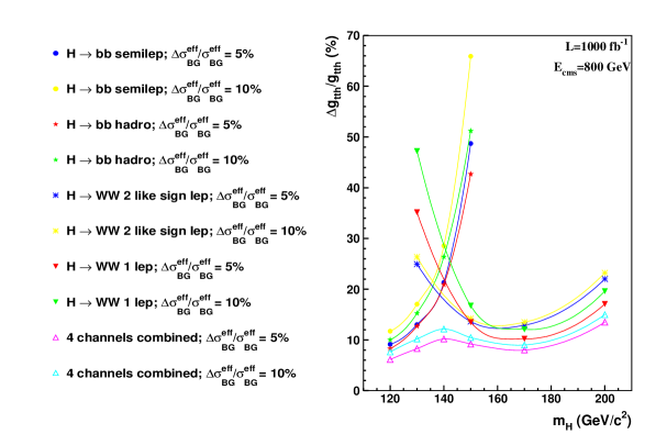
Figure 42: Top Yukawa coupling measurement expectations for a future 800 GeV $e^{+}e^{-}$ collider Gay:2006vs .

More sophisticated LC Higgs coupling analyses exist Hagiwara:2000tk , but aren’t often reviewed. They use a more complicated “optimal observables” (detailed kinematic shape information, for example) scheme. It’s more powerful, but doesn’t lend itself to the simplistic formulaic approach I just discussed.

I should emphasize that the results I reviewed are relevant only for the Standard Model. If the Higgs sector is non-minimal, or any new physics appears at the weak scale, it could result in altered couplings (and usually does; see Chapter IV). If they’re suppressed, the event rate goes down, resulting in greater uncertainty. This is often glossed over or ignored in discussions of Higgs phenomenology, but is a potential reality and something we’d just have to lump. Nevertheless, it should be clear by now that an ILC would be a spectacular experiment for precision Higgs measurements.

III.5 Higgs potential

Finally we arrive at the most difficult Higgs property to test, the potential. This is the hallmark of spontaneous symmetry breaking, thus ranks at least as high in priority as finding Yukawa couplings proportional to fermion masses. To see what’s involved, let’s review the SM Higgs potential. The potential is normally written as:

$$V(\Phi)=\mu^{2}\Phi^{\dagger}\Phi+\lambda(\Phi^{\dagger}\Phi)^{2}$$ (27)

where $\Phi$ is our $SU(2)_{L}$ complex doublet of scalar fields. The Higgs spontaneous symmetry-breaking mechanism is what happens to the Lagrangian when $\mu^{2}<0$ and the field’s global minimum shifts to $v=\sqrt{-\mu^{2}/\lambda}$. We then expand $\Phi\to v+H(x)$ (ignoring the Goldstone modes which you learned about in Sally Dawson’s lectures) where $H(x)$ is the radial excitation, the physical Higgs boson. The Higgs mass squared is then $2v^{2}\lambda$, and is the only free parameter, although constrained (weakly) by EW precision fits. The student performing this expansion will also notice $HHH$ and $HHHH$ Lagrangian terms, which are self-interactions of the Higgs boson. The three- and four-point couplings are $-6v\lambda$ and $-6\lambda$, respectively.

To measure the potential is to measure these self-couplings and check their relation to the measured Higgs mass. Our phenomenological approach is to rewire the Higgs potential in terms of independent parameters and the Higgs candidate field $\eta_{H}$:

$$V(\eta_{H})\;=\;\frac{1}{2}\,M^{2}_{H}\,\eta_{H}^{2}\,+\,\lambda\,v\,\eta_{H}^{3}\,+\,\frac{1}{4}\,\widetilde{\lambda}\,\eta_{H}^{4}$$ (28)

$\lambda$ and $\widetilde{\lambda}$ are now free parameters, which we measure from the direct production rate of $HH$ and $HHH$ events. This will ultimately be a voyage of frustration.

III.5.1 $HH$ production at LHC

We begin with Higgs pairs at LHC. The dominant production mechanism is gluon fusion, $gg\to HH$ Glover:1987nx ; Plehn:1996wb ; Dawson:1998py . The Feynman diagrams are shown in Fig. 43. The first diagram is off-shell single Higgs production which split via the three-point self-coupling to a pair of on-shell Higgses, which then decay promptly. The second diagram is a box (four-point)

Figure 43: Feynman diagrams for the dominant Higgs pair production rate at LHC, $gg\to HH$.

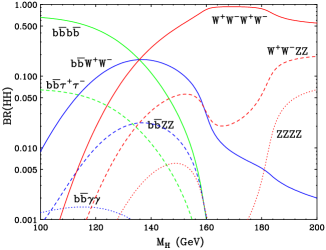
Figure 44: Left: Higgs pair production cross sections at LHC as a function of $M_{H}$ Djouadi:1999rc . Arrows show the change of the cross section as $\lambda$ is increase, and the tips are at one-half and twice the SM value. Right: Higgs pair branching ratios as a function of $M_{H}$, calculated using hdecay Djouadi:1997yw .

loop contribution which involves only the top quark Yukawa coupling. Interestingly, the two diagrams interfere destructively and have a rather large cancellation. This means the rate is small Djouadi:1999rc , as shown in Fig. 44, making our life difficult with a small statistical sample. On the other hand, the destructive interference will turn out to be crucial to making constructive statements about the self-coupling $\lambda$.

The left panel of Fig. 44 tells us that we can expect ${\cal O}(10k)$ light Higgs pair events per detector over the expected 300 fb^-1 lifetime of the first LHC run, and ten times that at SLHC. That sounds like a lot, but keep in mind that both Higgses have to decay to a final state we can observe, which will reduce the captured rate to something much smaller. Then we have to consider what backgrounds affect each candidate channel.

The right panel of Fig. 44 shows selected Higgs pair branching ratios. At low mass, decays to $b$ pairs dominate, as expected, while for $M_{H}\gtrsim 135$ GeV mass it’s $W$ pairs. We can immediately discount the $4b$ final state as hopeless, based on what we already learned about QCD backgrounds – but $4W$ is promising for higher masses. The next-largest mode from those two is $b\bar{b}W^{+}W^{-}$, which unfortunately is the same final state as the far larger top quark pair cross section. A few minutes’ investigation causes this to be discarded, even after trying various invariant mass constraints; $b$ pair mass resolution is just not good enough. The $b\bar{b}\tau^{+}\tau^{-}$ mode has very low backgrounds, comparable to the signal, but suffers hugely from lack of statistics, due to low efficiency for subsequent tau decays. However, the rare decay mode $b\bar{b}\gamma\gamma$ is extremely clean and worth further consideration at low masses.

$HH\to W^{+}W^{-}W^{+}W^{-}$ at LHC

$HH\to W^{+}W^{-}W^{+}W^{-}$ has myriad decays, but for triggering purposes and to get away from QCD background sources of leptons (like top quarks) we need to select special multilepton final states BPR_HH_4W . The most likely accessible channels are same-sign lepton pairs, $\ell^{\pm}\ell^{\pm}+4j$, and three leptons, $\ell^{+}\ell^{-}\ell^{\pm}+2j$, since the principal QCD SM backgrounds can’t easily mimic them. Note that because of multiple neutrinos departing the detector unobserved, complete reconstruction is not possible. The principle backgrounds are $WWWjj$, $t\bar{t}W$, $t\bar{t}j$, $t\bar{t}Z/\gamma^{*}$ and $WZ+4j$, but we also need to consider $t\bar{t}t\bar{t}$, $4W$, $W^{+}W^{-}+4j$, $W^{+}W^{-}Zjj$ as well as double parton scattering and overlapping events. The calculation of all of these is technical so I won’t go into it, rather simply mention a few noteworthy points.

The first is a warning about using the $gg\to HH$ effective Lagrangian in practical calculations. It is still a mystery why the leading term in the $\sqrt{\hat{s}}/m_{t}$ expansion Glover:1987nx should get the overall rate so close that of an exact calculation Plehn:1996wb , but it does. Because of that, nobody has ever bothered to calculate higher-order terms in the effective Lagrangian expansion; in any case, the exact results are available, as well as NLO in QCD Dawson:1998py . However, the leading terms in the expansion cancel too much close to threshold, yielding incorrect kinematics BPR_HH_4W , as can be seen from Fig. 45. One should thus use only the exact matrix element results for practical $gg\to HH$ phenomenology.

The second point is that our main systematic uncertainties will be our limited knowledge of the top quark Yukawa coupling, which drives the production rate, and the BR to $W^{+}W^{-}$, which drive the decay fraction. These must be known very precisely for any measurement to be useful.

Figure 45: Differential cross section as a function of the minimum jet pair lego plot separation for $\ell^{+}\ell^{-}+4j$ at events at LHC. The solid curve is the correct distribution using exact matrix elements for $HH$, while the dash-dotted curve comes from effective-Lagrangian matrix elements where the top quark mass is taken to infinity. Figure taken from Ref. BPR_HH_4W .

We will need a discriminating observable to separate signal from background. We can speculate that nearly all the signal’s kinematic information is encoded in the invariant mass of the visible final state particles, so let’s construct a new variable, $m_{vis}$:

$$m^{2}_{vis}\;=\;\left[\sum_{i}E_{i}\right]^{2}-\left[\sum_{i}\mathbf{p}_{i}\right]^{2}$$ (29)

where $i$ are all the leptons and jets in the event. We suspect a difference because the signal is a two-body process, which is threshold-like, while the backgrounds are multi-body processes which peak at much larger $m_{vis}$ than the sum of their heavy resonances’ masses.

Fig. 46 displays the fruits of parameterizing our ignorance (or rather, the detector’s). The separation between signal and background is exactly as expected: the signal peaks much lower, allowing a $\chi^{2}$ fit to distinguish it from the backgrounds. But the plot also reveals a saving grace in the destructive interference between triangle and box loop diagrams. If spontaneous symmetry breaking isn’t the right description and there is no Higgs potential, then $\lambda=0$ and the lack of destructive interference gives a wildly larger signal cross section, which is far easier to observe.

Fig. 47 summarizes the results of Ref. BPR_HH_4W . It plots $95\%$ CL limits on the shifted self-coupling, $\triangle\lambda=(\lambda-\lambda_{\rm SM})/\lambda_{\rm SM}$. This is somewhat easier to understand: zero is the SM, and -1 corresponds to no self-coupling, or no potential. For $M_{H}>150$ GeV, the LHC can exclude $\lambda=0$ at (for some $M_{H}$ much greater than) $2\sigma$ with only the LHC. After SLHC running, this becomes a $20-30\%$ measurement, if other systematics are under control. Here, they’re assumed to be smaller than the statistical uncertainty.

Figure 46: Visible invariant mass distribution for same-sign dilepton plus four jet event at LHC BPR_HH_4W . All SM backgrounds are summed into one curve, while the $gg\to HH$ signal is shown separately, for the SM value of self-coupling $\lambda$, twice that value, and zero.

Figure 47: $95\%$ CL limits achievable at LHC on the shifted Higgs triple self-coupling (see text), $\triangle\lambda$, for LHC and SLHC expected luminosities BPR_HH_4W .

Another potential systematics issue is minimum bias, the presence of extra jets in an event which don’t come from the primary hard scattering. Here, they could be confused with jets from the $W$ bosons, causing a distortion of $m_{vis}$. ATLAS has investigated this and found it to not be a concern – the shape of $m_{vis}$ for the signal remains largely unaltered Dahlhoff .

$HH\to b\bar{b}\gamma\gamma$ at LHC

We’ve already ruled out as viable the vast majority of Higgs pair BRs for $M_{H}\lesssim 150$ GeV due to QCD backgrounds or too-small efficiencies. However, the rare decay mode to $b\bar{b}\gamma\gamma$ is worth a closer look Baur:2003gp . There are many backgrounds to consider, coming from $b$ or $c$ jets plus photons, or other jets which fake photons, just as in the single Higgs to photon pairs case. Table 3 highlights the major ID efficiencies and fake photon rejection factors at LHC and SLHC relevant for us. The backgrounds are all calculable at LO, but with significant uncertainties, probably a factor of two or more. However, that won’t be a concern as we can identify distributions useful for measuring the background in the non-signal region. Note that with this channel we can completely reconstruct both Higgs bosons.

	$\epsilon_{\gamma}$	$\epsilon_{\mu}$	$P_{c\to b}$	$P_{j\to b}$	$P^{hi}_{j\to\gamma}$	$P^{lo}_{j\to\gamma}$
LHC	$80\%$	$90\%$	1/13	1/140	1/1600	1/2500
SLHC	$80\%$	$90\%$	1/13	1/23	1/1600	1/2500

Table 3: The major ID efficiencies and fake photon rejection factors at LHC. Note the two values for $P_{j\to\gamma}$, which represent the current uncertainty in detector capability for fake photon rejection. The true value won’t be known until data is collected. See Ref. Baur:2003gp for details.

Figure 48: Angular separations in the lego plot for $b$ jets and photons in $gg\to HH\to b\bar{b}\gamma\gamma$ signal events and background at the LHC. Figures from Ref. Baur:2003gp .

The background QCD uncertainties have a work-around. There are two angular distributions in the lego plot which look very different for the signal, principally because scalars decay isotropically and thus are uncorrelated, while the QCD backgrounds have spin correlations. The two distributions are shown in Fig. 48. The differences are rather dramatic (and even more so in 2-D distributions). Tevatron’s experiments CDF and DØ have used such a pseudo-sideband analysis for some time to measure a background in a non-signal region to normalize their Monte Carlo tools, then extrapolating to the signal region to perform a background subtraction. The technique is viable because QCD radiative corrections in general do not significantly alter angular distributions.

Table 4 summarizes the results of Ref. Baur:2003gp . It gives event rates expected with 600(6000) fb^-1 of data (two detectors) at LHC(SLHC). SLHC would not get ten times as many events because of lower efficiency of having to tag two $b$ jets instead of only one, to overcome the low fake jet rejection rate in a high-luminosity environment. First, note that fake $b$ jets or fake photons are the largest background: the measurement would be significantly hampered by detector limitations. Second, while the $S/B$ ratio is excellent, the overall event rate is extremely small, definitely in the non-Gaussian statistics regime.

SLHC could make a useful statement about $\lambda$, ultimately achieving limits on $\triangle\lambda$ of about $\pm 0.5$, but this is not such a strong statement. It could at best generally confirm the SM picture of spontaneous symmetry breaking and perhaps rule out wildly different scenarios, but would never be particularly satisfying. On the other hand, it’s strong encouragement for ATLAS and CMS to push the envelope on tagging efficiency and fake rejection, especially for the detector upgrades necessary for SLHC. Doing studies like this well ahead of time is useful for this reason, our present case being a perfect example.

	$HH$	$b\bar{b}\gamma\gamma$	$c\bar{c}\gamma\gamma$	$b\bar{b}\gamma j$	$c\bar{c}\gamma j$	$jj\gamma\gamma$	$b\bar{b}jj$	$c\bar{c}jj$	$\gamma jjj$	$jjjj$	$\sum({\rm bkg})$	S/B
LHC	6	2	1	1	0	5	0	0	1	1	11	1/2
SLHC	21	6	0	4	0	6	1	0	1	1	20	1/1

Table 4: Expected event rates after ID efficiencies and all kinematic cuts for $b\bar{b}\gamma\gamma$ events at LHC (SLHC), two detectors and 600(6000) fb^-1 of data Baur:2003gp . LHC assumes only one $b$ tag, while SLHC requires two. Note the increased fake rate at SLHC.

III.5.2 $HH$ production at an ILC

While (S)LHC clearly has access to Higgs pair production and thus $\lambda$ for $M_{H}>150$ GeV, it would disappoint at lower masses. We should see if a future linear collider could also give a precision measurement for $\lambda$ as it could for (most) other Higgs couplings.

For $e^{+}e^{-}$ collisions below about 1 TeV, double Higgsstrahlung is the largest source of Higgs pairs. The Feynman diagrams appear in Fig. 49, while the cross sections as a function of $M_{H}$ for 500 and 800 GeV collisions Djouadi:1999gv are found in Fig. 50, which also shows the cross sections times BRs for the dominant final states over the range of Higgs masses. Roughly, this corresponds to $4b$ and $4W$ final state. The former is very steeply falling with $M_{H}$, but the latter is much flatter over the 100–200 GeV mass region, suggesting broader access if at all visible.

The parton-level studies performed so far Baur:compare are fairly encouraging. As shown in Fig. 51, an ILC could achieve about a $20-30\%$ measurement of $\lambda$ over a broad mass range, with somewhat worse performance around $M_{H}\sim 140$ GeV, where the $b\bar{b}$ and $W^{+}W^{-}$ BRs are roughly equal. Interestingly, for a lower Higgs mass, the analysis prefers lower machine energy, while the opposite is true at least to a small degree at higher mass. This is largely a phase space effect for the 3-body production mechanism. Also, SLHC is superior for $M_{H}\gtrsim 150$ GeV (largely due to better statistics), with an important caveat: controlling systematics in $gg\to HH\to 4W$ at LHC would require precision input from ILC for the Higgs couplings and BRs. This is an excellent example of synergy between experiments.

Figure 49: Feynman diagrams for double Higgsstrahlung at a future linear collider, $e^{+}e^{-}\to HH$.

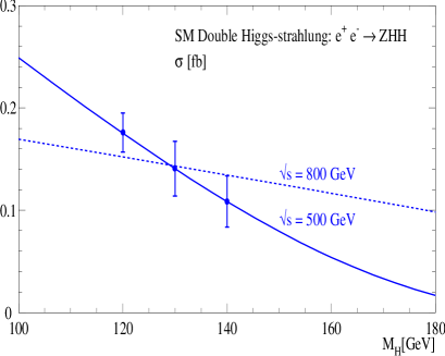
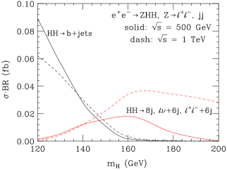
Figure 50: Left: the double Higgsstrahlung cross section as a function of $M_{H}$ for 500 and 800 GeV $e^{+}e^{-}$ collisions Djouadi:1999gv . Right: the cross section times BR at 500 GeV and 1 TeV $e^{+}e^{-}$ collisions, for the dominant final state BRs as a function of $M_{H}$ Baur:compare .

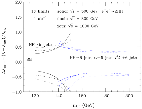
Figure 51: Estimated achievable limits in the shifted self-coupling $\triangle\lambda$ (see Sec. III.5.1) at future $e^{+}e^{-}$ colliders of various energy, as a function of $M_{H}$ Baur:compare .

Double Higgsstrahlung is not the only source of Higgs pairs at an $e^{+}e^{-}$ collider, however. In fact, as the energy increases, WBF Higgs pair production becomes more and more important. Representative Feynman diagrams for $e^{+}e^{-}\to\nu\bar{\nu}HH$ are shown in Fig. 52. A preliminary analysis DeRoeck:2004zu for CLIC Accomando:2004sz , a second-generation $1-5$ TeV $e^{+}e^{-}$ collider collecting 5000 fb^-1, found rather interesting results, summarized graphically in Fig. 53. The principal finding is that no matter how high the collision energy goes, and regardless of Higgs mass, the precision on $\lambda$ bottoms out at $10-15\%$. This is because the self-coupling has an $s$-channel suppression, and its contributions becomes washed out as by other diagrams as $\sqrt{s}$ increases. A corollary, though, is that CLIC could potentially achieve better precision than SLHC for larger $M_{H}$, although this may be marginal. Much more detailed work would be required for both SLHC and CLIC, as well as experience at LHC and SLHC to determine its true potential, to make conclusive statements.

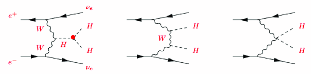
Figure 52: Representative Feynman diagrams for the WBF process $e^{+}e^{-}\to\nu\bar{\nu}HH$.

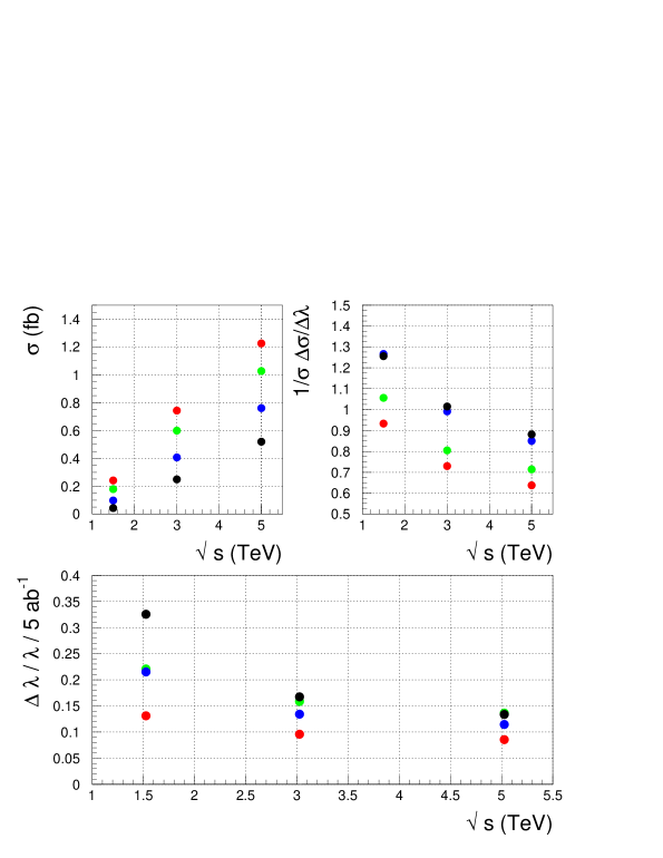
Figure 53: The results of Ref. DeRoeck:2004zu for WBF $HH$ production at CLIC, a second-generation multi-TeV $e^{+}e^{-}$ collider. The plot labels are self-explanatory, while the colors are for various Higgs masses: 120 GeV in red, 140 GeV in blue, 180 GeV in green and 240 GeV in black.

III.5.3 Electroweak corrections to $\lambda$

One final word on the trilinear self-coupling $\lambda$: Ref. Kanemura:2002vm calculated the leading 1-loop top quark EW corrections to $\lambda_{\rm SM}$. Their principal SM result is:

$$\lambda^{eff}_{HHH}\;=\;\frac{M^{2}_{H}}{2v^{2}}\left[1-\frac{N_{C}}{3\pi^{2}}\frac{m^{4}_{t}}{v^{2}M^{2}_{H}}+...\right]$$ (30)

The correction is $-10\%$($-4\%$) for $M_{H}=120(180)$ GeV, non-trivial for smaller Higgs masses, but those are excluded in the SM. This correction should obviously be taken into account in any future analysis, should the Higgs be found. But it should be clear that neither (S)LHC nor ILC will be sensitive to it. Even CLIC would have only marginal sensitivity, and then only for low $M_{H}$.

Non-minimal Higgs sectors and new physics effects can tell a very different story, however, as we’ll see, coming up in Secs. IV.1 and IV.5.

III.5.4 $HHH$ production anywhere

The trilinear self-coupling $\lambda$ is only part of our phenomenological Higgs potential of Eq. 28, though. We also need to measure $\widetilde{\lambda}$, the quartic self-coupling. In some sense this is equally important to measuring $\lambda$. Recall the structure of the Higgs potential: $\lambda$ allows the global minimum to be away from zero, but a non-zero (and positive) $\widetilde{\lambda}$ is required to keep the potential bounded from below. We can’t really convince ourselves that the potential structure of Eq. 27 is the right picture without a measurement of both these ingredients. We’ve just seen that probing $\lambda$ is extremely challenging. Just how difficult is this likely to be for $\widetilde{\lambda}$?

For $e^{+}e^{-}$ collisions we already know this is hopeless: the $HHH$ rate is both too low and its dependence on $\widetilde{\lambda}$ too weak Djouadi:1999gv . However, the situation at (S)LHC was only very recently investigated Plehn:2005nk ; Binoth:2006ym . The authors calculated the $gg\to HHH$ cross section, which involves Feynman diagrams like those of Fig. 54. Note the appearance of numerous diagrams dependent on the trilinear self-coupling, in addition to diagrams dependent only on $y_{t}$.

The results of the study are shown in Fig. 55, for a 200 TeV VLHC. They’re rather deflating because the cross section is miserably small. A challenge to the student: find a three-Higgs BR to a final state that could be observed at a VLHC, where the rate is not laughable. Good luck! In addition, the right panel shows that any variation of the trilinear coupling $\lambda$ completely swamps variation of the quartic $\widetilde{\lambda}$, whose own variation is already infinitesimal.

In summary, it appears that we will likely never achieve a complete picture of the Higgs potential. This of course applies only to the Standard Model. Coming up in Chapter IV we’re going to see that for BSM physics the situation is even more discouraging.

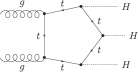
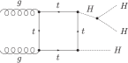
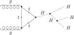
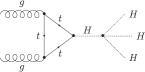
Figure 54: Representative Feynman diagrams for $gg\to HHH$.

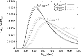
Figure 55: Left: 200 TeV VLHC $gg\to HHH$ cross section as a function of $M_{H}$. Right: differential cross section as a function of $M_{HHH}$ for three values each of $\lambda$ and $\widetilde{\lambda}$. Figures from Ref. Plehn:2005nk .

IV Beyond-the-SM Higgs sectors

Now that we know how the Standard Model Higgs sector works – how it could be discovered and measured at LHC – it’s natural to think about other possibilities for EWSB. The SM Higgs is elegant in its simplicity, but as you know from Sally Dawson’s SM lectures, it’s probably too minimal – nagging theoretical questions remain about Higgs mass stability, flavor (ignoring this is kind of a black eye), neutrino masses (another black eye), and so on. Because new physics that could explain dark matter is likely to also lie at the TeV scale, most model building makes an attempt to incorporate solutions to some of these other problems along with EWSB. The literature is vast, but let’s try to roughly classify some of the major ideas to get a handle on the variations.

The broadest two categories of classes are weakly-coupled new physics which can be handled with perturbation theory, and strongly-coupled or “strong dynamics” models which are penetrable in some cases, others not. These include QCD-inspired theories like Technicolor Weinberg:1975gm ; Susskind:1978ms (or more properly Extended Dimopoulos:1979es ; Eichten:1979ah or Walking Holdom:1981rm Technicolor, which can handle a top quark mass very different from the other quark masses) and Topcolor-assisted Technicolor TC2 (“TC2”), which incorporates additional weakly-coupled gauge structure. Strong dynamics assumes that some TeV-scale massive or heavier fermions’ attraction became strong at low energy scales, eventually causing their condensation to mesonic states (Technipions, Technirho, Technieta, etc.), the neutral scalars of which can incite EWSB via their $SU(2)_{L}$ gauge interactions. Strong dynamics scenarios are beyond the scope of these lectures, however, so I leave it for the interested student to study the excellent review article of Ref. Hill:2002ap .

While strong dynamics theories are Higgsless in some sense, meaning no fundamental scalar fields, the terms is usually reserved for a new class of models where the EW symmetry is broken using boundary conditions on gauge boson wavefunctions propagating in finite extra dimensions (see e.g. Refs. Simmons:2006iw ; Cacciapaglia:2004zv ). We’ll also skip these.

There is far more theoretical effort expended on weakly-coupled EWSB, which is mostly variations on what we can add to the single Higgs doublet of the SM:

1. 1HDM + invisible (high-scale) new physics, hidden from direct detection

2. CP-conserving 2HDM: 4 types (minimal supersymmetry, MSSM, is Type II)

3. CP-violating 2HDM

4. Higgs singlet(s) (e.g. next-to-minimal supersymmetry, NMSSM)

5. Higgs triplets (often appear in Grand Unified Theories)

6. Little Higgs models: $SU(2)_{L}\times U(1)_{Y}$ is part of larger gauge and global group

The first item, new high-scale physics hidden from direct detection, sounds like a cheat. It actually involves an important aspect of phenomenology: effective Lagrangians from higher-dimensional operators. We’ll come back to these in a moment. Two Higgs doublets instead of one is an idea with multiple sources. For instance, one doublet could give mass to the leptons and the other to the quarks, or one to the up-type fermions and the other to the down-type, etc. We’ll return to these after effective operators. Additional Higgs singlets likewise have a variety of reasons for being written down, but usually it’s just “we can do it, so we will”. We’ll skip these. Higgs triplets originated from natural appearance in left-right symmetric GUTs. They’re a bit exotic and typically have issues with precision EW data, but are interesting in that they predict the existence of doubly-charged Higgs states $H^{\pm\pm}$, and a tree-level $H^{\pm}W^{\mp}Z$ coupling, which must be zero in most Higgs-doublet models. It would therefore stand out experimentally. For all these cases I don’t have time to cover, the Higgs Hunter’s Guide is the best place to start to learn more HHG .

Little Higgs theories, on the other hand, are different in that they necessarily involve new scalar and gauge structure arising from an enlarged global symmetry from which the SM emerges, as well as additional matter content. Interestingly, in these models the Higgs looks very much like the SM Higgs, but with ${\cal O}(v^{2}/F^{2})$ corrections, where $F$ is typically a few TeV, parametrically $4\pi$ larger than the EW scale. The smallness of $v^{2}/F^{2}$ could make it very difficult to measure Little Higgs corrections to Higgs observables. These models are probably ultimately strongly-coupled at a scale $\Lambda\sim 4\pi F$, but this is an open question. If nature chose this course, the most interesting physics is the new gauge boson and matter fields that appears at a scale $F$. Refs. LH-reviews provide nice overviews and simple explanations of the two primary Little Higgs mechanisms.

IV.1 Higher-dimensional operators

The new physics responsible for dark matter, flavor, neutrino masses, etc., might very well be too massive to produce directly at colliders. This the dreaded SM-Higgs-only scenario, where LHC sees nothing new. It would really be an invitation to take a more rigorous look at all data – new physics effects might still appear as small deviations in precision observables.

The standard way of parameterizing this is to write down all the possible Lagrangian operators with the heavy fields integrated out which preserve $SU(3)_{c}\times SU(2)_{L}\times U(1)_{Y}$ gauge invariance. This was done over two decades ago for operators up to dimension six Buchmuller:1985jz . Although not often emphasized in today’s phenomenology, I consider this paper a must-read for all students.

Let’s begin by considering the possible operators involving only the SM Higgs doublet. There are two, of dimension six:

$${\cal O}_{1}=\frac{1}{2}\,\partial_{\mu}\,(\Phi^{\dagger}\Phi)\,\partial^{\mu}(\Phi^{\dagger}\Phi)\qquad\&\qquad{\cal O}_{2}=-\frac{1}{3}\,(\Phi^{\dagger}\Phi)^{3}$$ (31)

for the effective Lagrangian contribution

$${\cal L}_{6D,\Phi}\;=\;\sum\limits^{2}_{i=1}\frac{f_{i}}{\Lambda^{2}}{\cal O}_{i}\;,\;\;f_{i}>0$$ (32)

$\Lambda$ must be at least a couple TeV, otherwise we’d likely observe it directly at LHC. If you’ve somewhere seen an alternative effective theory for the Higgs potential written as

$$V_{\rm eff}\;=\;\sum\limits_{n=0}\frac{\lambda_{n}}{\Lambda^{2n}}\biggl{(}|\Phi|^{2}-\frac{v^{2}}{2}\biggr{)}^{2+n}$$ (33)

the operators written above correspond to the $n=1$ term in this expansion.

${\cal O}_{1}$ modifies the Higgs kinetic term, while ${\cal O}_{2}$ modifies the EW vev, $v$:

$${\cal L}_{\rm kin}\;=\;\frac{1}{2}\,\partial_{\mu}\phi\,\partial^{\mu}\phi+\frac{1}{2}f_{1}\frac{v^{2}}{\Lambda^{2}}\,\partial_{\mu}\phi\,\partial^{\mu}\phi\;,\qquad\frac{v^{2}}{2}\;\approx\;\frac{v^{2}_{0}}{2}\bigl{(}1-\frac{f_{2}}{4\lambda}\frac{v^{2}_{0}}{\Lambda^{2}}\bigr{)}$$ (34)

where $v$ is what $G_{F}$ measures. We must also canonically normalize the physical Higgs field: $\phi=NH$ with $N=1/(1+f_{1}\frac{v^{2}}{\Lambda^{2}})$.

This results in a number of alterations to masses and couplings Barger:2003rs . First, the Higgs mass itself receives corrections from the expected value, given $\lambda$:

$$M_{H}^{2}\;=\;2\lambda v^{2}\bigl{(}1-f_{1}\frac{v^{2}}{\Lambda^{2}}+\frac{f_{2}}{2\lambda}\frac{v^{2}}{\Lambda^{2}}\bigr{)}$$ (35)

where the $f_{2}$ term is independent of $\lambda$. Next, Higgs gauge couplings receive $v^{2}/\Lambda^{2}$ shifts:

$$\frac{1}{2}g^{2}v\biggl{(}1-\frac{f_{1}}{2}\frac{v^{2}}{\Lambda^{2}}\biggr{)}HW^{+}_{\mu}W^{-\mu}\;\; \;\;\frac{1}{4}g^{2}\bigl{(}1-f_{1}\frac{v^{2}}{\Lambda^{2}}\bigr{)}HHW^{+}_{\mu}W^{-\mu}$$ (36)

$$\frac{1}{2}\frac{g^{2}}{c_{W}}v\biggl{(}1-\frac{f_{1}}{2}\frac{v^{2}}{\Lambda^{2}}\biggr{)}HZ_{\mu}Z^{\mu}\;\; \;\;\frac{1}{4}\frac{g^{2}}{c_{W}}\bigl{(}1-f_{1}\frac{v^{2}}{\Lambda^{2}}\bigr{)}HHZ_{\mu}Z^{\mu}$$

Finally, the Higgs boson self-couplings are (phases vary with Feynman rule convention):

$$|\lambda_{3H}|=\frac{3m^{2}_{H}}{v}\left[\left(1-\frac{f_{1}}{2}\frac{v^{2}}{\Lambda^{2}}+\frac{2f_{2}}{3}\frac{v^{2}}{M^{2}_{H}}\frac{v^{2}}{\Lambda^{2}}\right)+\frac{2f_{1}}{3M^{2}_{H}}\frac{v^{2}}{\Lambda^{2}}\sum_{i<j}^{3}p_{i}\cdot p_{j}\right]$$ (37)

$$|\lambda_{4H}|=\frac{3m^{2}_{H}}{v^{2}}\left[\left(1-f_{1}\frac{v^{2}}{\Lambda^{2}}+4f_{2}\frac{v^{2}}{M^{2}_{H}}\frac{v^{2}}{\Lambda^{2}}\right)+\frac{2f_{1}}{3M^{2}_{H}}\frac{v^{2}}{\Lambda^{2}}\sum_{i<j}^{4}p_{i}\cdot p_{j}\right]$$ (38)

Note that ${\cal O}_{1}$ and ${\cal O}_{2}$ both enter here, but more importantly there are momentum-dependent terms, which are typical of higher-dimensional operators. The effect of these terms would be anomalous high-$p_{T}$ Higgses in pair production.

Only one phenomenological analysis exists for these effects, and only for precision experiments at a future ILC and CLIC Barger:2003rs . In this study, measurements are expressed in terms of $a_{i}=f_{i}\,v^{2}/\Lambda^{2}$, since $f_{i}$ and $\Lambda$ can’t be easily separated from so few measurements. Higgsstrahlung, double Higgsstrahlung and WBF Higgs pair production together measure a combination of $a_{1}$ and $a_{2}$.

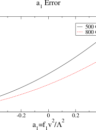
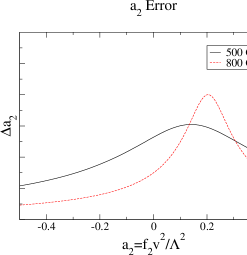
Figure 56: Achievable uncertainty on measurements of the $a_{1}$ (left) and $a_{2}$ (right) coefficients of Eq. 31 (also see text) at a future ILC for 500 and 800 GeV running Barger:2003rs .

Fig. 56 shows the expected achievable uncertainties (not limits!) on $a_{1}$ and $a_{2}$ at a future ILC. For $f_{1}=1$, this corresponds to a reach in $\Lambda$ of about 4 TeV, possibly out of the reach of LHC depending on what might be directly produced. For $f_{2}=1$, however, this corresponds to only about $\Lambda\sim 0.8$ TeV, easily accessible at LHC. Put another way, an ILC could have access to new high-scale physics via altered Higgs–gauge boson couplings, but not via Higgs self-couplings. This is in line with what we’d come to expect, as $HH$ production is much smaller. The shapes of the uncertainty curves in the figures depend on what values of the operator coefficients add to or subtract from the signal, with the added feature that the momentum dependence of the Higgs self-couplings that the ${\cal O}_{1}$ operator introduces changes to kinematic distributions.

In addition to the Higgs-only D6 operators, there are a handful of operators involving the Higgs and gauge boson fields together Buchmuller:1985jz :

$O_{WW}\;=\;(\phi^{\dagger}\phi)\bigl{[}W^{+}_{\mu\nu}W^{-\mu\nu}+\frac{1}{2}W^{3}_{\mu\nu}W^{3\mu\nu}\bigr{]}$

$O_{BB\phantom{h}}\;=\;(\phi^{\dagger}\phi)B_{\mu\nu}B^{\mu\nu}$

$O_{BW\phantom{i}}\;=\;B^{\mu\nu}\bigl{[}(\phi^{\dagger}\sigma^{3}\phi)W^{3}_{\mu\nu}+\sqrt{2}\bigl{[}(\phi^{\dagger}T^{+}\phi)W^{+}_{\mu\nu}+(\phi^{\dagger}T^{-}\phi)W^{-}_{\mu\nu}\bigr{]}\bigr{]}$

$O_{B\phantom{Bh}}\;=\;(D^{\mu}\phi)^{\dagger}(D^{\nu}\phi)B_{\mu\nu}$

$O_{W\phantom{Bi}}\;=\;(D^{\mu}\phi)^{\dagger}\bigl{[}\sigma^{3}(D^{\nu}\phi)W^{3}_{\mu\nu}+\sqrt{2}\bigl{[}T^{+}(D^{\nu}\phi)W^{+}_{\mu\nu}+T^{-}(D^{\nu}\phi)W^{-}_{\mu\nu}\bigr{]}\bigr{]}$

$O_{\Phi,1\phantom{w}}\;=\;(D_{\mu}\phi)^{\dagger}\phi\phi^{\dagger}(D^{\mu}\phi)$

These induce momentum-dependent $HHVV$ vertices, so could be studied at an ILC or CLIC in the same manner as the Higgs-only couplings, as well as with rare Higgs decays Hagiwara:1993qt , but in general they’re highly constrained by EW precisions observables ($S$, $\rho$, $g_{VVV}$) Hagiwara:1995vp . Interestingly, it appears there has not been an update of the EW constraints on these operators since 1997 Szalapski:1997rf , although there are predictions for limits at an ILC Beyer:2006hx . There is, however, a new analysis for WBF Higgs at LHC includes the effects of some of these operators and finds that they would be encoded in the tagging jet azimuthal separation Hankele:2006ma .

There is also a set of D6 operators involving the Higgs, fermion and gauge boson fields Buchmuller:1985jz :

$O_{d\phi}\;\,=\;(\phi^{\dagger}\phi)(\bar{q}d\phi)$	$O_{\phi d}\;\,=\;i(\phi^{\dagger}D_{\mu}\phi)(\bar{d}\gamma^{\mu}d)$	$O_{\bar{D}d}\;=\;(D_{\mu}\bar{q}d)D^{\mu}\phi$
$O^{(1)}_{\phi q}\;=\;i(\phi^{\dagger}D_{\mu}\phi)(\bar{q}\gamma^{\mu}q)$	$O_{\phi\phi}\>\,=\;i(\phi^{\dagger}\epsilon D_{\mu}\phi)(\bar{u}\gamma^{\mu}d)$	$O_{dW}\,=\;(\bar{q}\sigma^{\mu\nu}\sigma^{i}d)\phi W^{i}_{\mu\nu}$
$O^{(3)}_{\phi q}\;=\;i(\phi^{\dagger}D_{\mu}\sigma^{i}\phi)(\bar{q}\gamma^{\mu}\sigma^{i}q)$	$O_{Dd}\;=\;(\bar{q}D_{\mu}d)D^{\mu}\phi$	$O_{dB}\>\,=\;(\bar{q}\sigma^{\mu\nu}d)\phi B_{\mu\nu}$

Some of these are constrained by precise LEP measurements of $Zb\bar{b}$, $\gamma b\bar{b}$ couplings, but not severely. They would give interesting rare Higgs decays like $H\to b\bar{b}Z,b\bar{b}\gamma$. Their phenomenology for LHC and even ILC is not really studied. Thus, I can’t say to what scale they might be sensitive given a SM Higgs discovery with nothing else observed.

IV.2 Two-Higgs doublet models (2HDMs)

The most-often studied extension to the SM Higgs sector is the two-Higgs doublet model (2HDM) Lee:1973iz ; HHG . That is, we add one additional $SU(2)_{L}$ doublet. Both of the doublets acquire a vev. For now let’s assume CP conservation and work with in the real-vev basis. Counting degrees of freedom, four per complex doublet, and knowing that three modes are “eaten” to give the $W^{\pm}$ and $Z$ their masses, after SSB there must be five physical states. Two of them will necessarily be charged ($H^{\pm}$) regardless of how we assigned hypercharge to each doublet, leaving the other three neutral. Of those, two ($h$, $H$) will be CP-even and one will be CP-odd ($A$), the last of which won’t couple to the weak bosons at tree level. The general 2HDM potential is quite messy CTHill ; HHG , so we’ll not discuss it.

Recall the primary role of the Higgs sector: to restore unitarity to weak boson scattering. This requires the gauge coupling to $WW$ to be exactly $\frac{1}{2}g_{W}^{2}v$, where $v$ is what we measure with $G_{F}$. In the amplitude, then, the coupling squared is $\frac{1}{4}g_{W}^{4}v^{2}$. With two vevs, there is the automatic constraint $v_{1}^{2}+v_{2}^{2}\equiv v^{2}$ Huffel:1980sk . The ratio is $\tan\beta\equiv\frac{v_{2}}{v_{1}}$. The CP-even mass eigenstates, which couple to the weak bosons, thus boil down to simply mixing:

$$h\;\;=\;\sqrt{2}\bigl{[}-({\rm Re}\phi^{0}_{1}-v_{1})\sin\alpha+({\rm Re}\phi^{0}_{2}-v_{2})\cos\alpha\bigr{]}$$ (39)

$$H\;=\;\sqrt{2}\bigl{[}\phantom{-}({\rm Re}\phi^{0}_{1}-v_{1})\cos\alpha+({\rm Re}\phi^{0}_{2}-v_{2})\sin\alpha\bigr{]}$$ (40)

where $\alpha$ is the angle which diagonalizes the $2\times 2$ mixing matrix. The Higgs sector is typically defined by $\alpha$, $\tan\beta$ and the potential parameters which govern the self-couplings. Some models are defined instead by $M_{A}$ and $M_{Z}$.

Let’s pause for a moment to reflect on what would happen if we introduced CP violation Lee:1973iz . This is a well-motivated exercise since there isn’t enough CP violation in the SM model to account for baryogenesis in the early universe. The most immediate impact is that $h$, $H$ and $A$ now mix. $M_{A}$ is supposed to parameterize the pseudoscalar pole, but it’s now mixed into three physical states, so it becomes ill-defined. Instead, we typically use the charged Higgs mass. It would be logical to use $M_{H^{\pm}}$ for CP-conserving scenarios as well, but this is one of those historical accidents that has too much momentum to change.

Regarding the fermions, we can apportion the two doublets in four general ways HHG :

• only $\Phi_{2}$ couples to fermions

• $\Phi_{1}$ couples to down-type, $\Phi_{2}$ to up-type fermions

• $\Phi_{1}$ couples to down quarks, $\Phi_{2}$ to up quarks and down leptons

• $\Phi_{1}$ couples to quarks, $\Phi_{2}$ to leptons

Types III and IV induce flavor-changing neutral currents (FCNCs), which are highly constrained, thus these models are not much studied any more. Types I and II are qualitatively different and worth a quick look at the differences in their couplings, shown in Table 5. Because of which doublet gives the down-type fermions their masses, those Yukawa couplings to $h$ and $H$ are swapped between models, with a phase factor from mixing. Similarly, the $Af\bar{f}$ coupling is inverted and changes sign: $\cot\beta\to-\tan\beta$. The gauge coupling for $h$ and $H$, of course, are unaffected by the Yukawa couplings and are fixed to $\sin(\beta-\alpha)$ and $\cos(\beta-\alpha)$. (The sum of their squares in the amplitude must equal 1!)

The charged Higgs Yukawa couplings are slightly different yet. The left-handed coupling is proportional to the up-type Yukawa coupling, and the right-handed coupling the down-type Yukawa, for an out-flowing $H^{-}$. The reverse is true for an outflowing $H^{+}$. We have:

$$g_{H^{-}D\bar{U}}\;=\;\frac{g}{2\sqrt{2}M_{W}}\bigl{[}m_{U}\cot\beta(1+\gamma_{5})-m_{D}\cot\beta(1-\gamma_{5})\bigr{]}$$ (41)

$$g_{H^{-}D\bar{U}}\;=\;\frac{g}{2\sqrt{2}M_{W}}\bigl{[}m_{U}\cot\beta(1+\gamma_{5})+m_{D}\tan\beta(1-\gamma_{5})\bigr{]}$$ (42)

where $H^{-}$ flows out, $D$ is incoming and $\bar{U}$ is outgoing.

$\Phi$	$\frac{g_{\Phi u\bar{u}}}{g_{f}}$	$\frac{g_{\Phi d\bar{d}}}{g_{f}}$	$\frac{g_{\Phi VV}}{g_{V}}$	$\frac{g_{\Phi ZA}}{g_{V}}$
$h$	$-\frac{\cos\alpha}{\sin\beta}$	$-\frac{\cos\alpha}{\sin\beta}$	$\sin(\beta-\alpha)$	$-\frac{1}{2}i\cos(\beta-\alpha)$
$H$	$-\frac{\sin\alpha}{\sin\beta}$	$-\frac{\sin\alpha}{\sin\beta}$	$\cos(\beta-\alpha)$	$\phantom{-}\frac{1}{2}i\sin(\beta-\alpha)$
$A$	$-i\gamma_{5}\cot\beta$	$i\gamma_{5}\cot\beta$	0	0
$h$	$-\frac{\cos\alpha}{\sin\beta}$	$\phantom{-}\frac{\sin\alpha}{\cos\beta}$	$\sin(\beta-\alpha)$	$-\frac{1}{2}i\cos(\beta-\alpha)$
$H$	$-\frac{\sin\alpha}{\sin\beta}$	$-\frac{\cos\alpha}{\cos\beta}$	$\cos(\beta-\alpha)$	$\phantom{-}\frac{1}{2}i\sin(\beta-\alpha)$
$A$	$-i\gamma_{5}\cot\beta$	$-i\gamma_{5}\tan\beta$	0	0

Table 5: Fermion and gauge boson couplings in Type I (upper) and II (lower) 2HDMs.

IV.3 Type II 2HDM in the MSSM

At this point we should focus on the Type II 2HDM, because that’s the one required to appear in the MSSM (see Ref. JackHowie_MSSM_H for a detailed description). Model I will have similar features, modulo the couplings swaps given in Table 5, so is understandable by analogy. We’ll spend the remaining portion discussing only SUSY Higgs phenomenology, and specifically minimal SUSY, the MSSM. However, by the end it should be apparent that extended Higgs sectors may often be treated as variations on a theme, with much of the phenomenology based on the same collider signatures.

The MSSM imposes tree-level constraints on the Higgs potential which require the various $\lambda$ to be gauge parameters (MSSM extensions add non-gauge terms). We’ll come back to what the potential looks like in Sec. IV.5 and study its phenomenology, and for now simply examine the implication of this structure on the mass spectrum. Because we consider only the CP-conserving case here, we can get away with using $M_{A}$ as an input. The others will be $\tan\beta$ as discussed before, the average top squark mass $M_{S}$, and an encoded trilinear mixing parameter for the top sector, $X_{t}$. This last one is important because of the large top Yukawa corrections the MSSM Higgs sector receives. The values $0$ and $\sqrt{6}\,M_{S}$ are referred to as “no mixing” and “maximal mixing”, because they extremize the loop corrections. The $h-H$ mixing angle is

$$\alpha\;=\;\frac{1}{2}\tan^{-1}\biggl{[}\tan 2\beta\frac{M_{A}^{2}+M_{Z}^{2}}{M_{A}^{2}-M_{Z}^{2}}\biggr{]}\;,\qquad-\frac{\pi}{2}\leq\alpha\leq 0$$ (43)

to first order. The CP-even masses are given by:

$$M^{2}_{H,h}\;=\; \frac{1}{2}\biggl{(}M^{2}_{A}+M^{2}_{Z}\pm\sqrt{(M_{A}^{2}+M_{Z}^{2})^{2}+4M_{A}^{2}M_{Z}^{2}\sin^{2}(2\beta)}\biggr{)}$$

$$+\frac{3}{8\pi^{2}}\cos^{2}\alpha\>y_{t}^{2}m_{t}^{2}\biggl{[}\log\frac{M_{S}^{2}}{m_{t}^{2}}+\frac{X_{t}^{2}}{M_{S}^{2}}\biggl{(}1-\frac{X_{t}^{2}}{12M_{S}^{2}}\biggr{)}\biggr{]}\;\;\;\;{\rm for}\,M_{h}\,{\rm only}$$

where the top Yukawa correction can be significant, a couple tens of GeV. The charged Higgs mass is rather more simple:

$$M_{H^{\pm}}^{2}=M_{A}^{2}+M_{W}^{2}$$ (45)

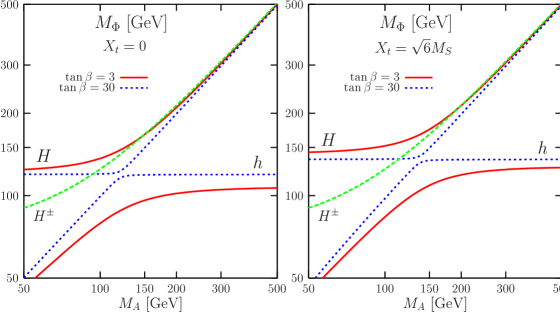
Figure 57: MSSM Higgs boson masses as a function of pseudoscalar mass $M_{A}$ and two choices of $\tan\beta$, for no (left) and maximal (right) mixing ($X_{t}$ parameter; see text). Figures from Ref. Djouadi .

These equations exhibit the interesting property of $h$ decoupling with increasing pseudoscalar mass: for large $M_{A}$ the heavy states $H$, $A$ and $H^{\pm}$ tend to be closely degenerate, and the light $h$ has an asymptotic maximum mass which depends mostly on $\tan\beta$. We see this behavior, along with a plateau effect for $M_{h}$ and $M_{H}$, in Fig. 57. There is always at least one CP-even Higgs boson in the mass region $90\lesssim M_{\phi}\lesssim 145$ GeV, assuming perturbativity to high scales. For large $M_{A}$, toward the decoupling region, it is the lighter state, $h$, but at low $M_{A}$ it is the heavier state, $H$. The transition region is sharper for larger $\tan\beta$.

The mass spectrum is not the only feature to exhibit the decoupling and transition behavior, however. Both the gauge and Yukawa couplings do the same. The $VV\phi$ couplings are shown in Fig. 58. By comparison with Fig. 57, we easily see that when either $h$ or $H$ is in its plateau mass region, it holds most of the gauge coupling; $\sin(\beta-\alpha)\to 1$ or $\cos(\beta-\alpha)\to 1$. In the transition region, the two states share the gauge coupling, and both are of comparable importance in unitarity cancellation. As with the mass spectrum, and by now as anticipated, the transition region is sharper for larger $\tan\beta$. Hold these two figures in your mind, as they are going to play an extremely important phenomenological role shortly.

Using just trigonometry, let’s rewrite the Yukawa couplings of Table 5 to see better how they depend on $M_{A}$ and $\tan\beta$:

$$g_{hu\bar{u}}= -\frac{\cos\alpha}{\sin\beta}\,Y_{u} =\;-[\sin(\beta-\alpha)+\cot\beta\cos(\beta-\alpha)]\>Y_{u}$$ (46)

$$g_{hd\bar{d}}= \phantom{-}\frac{\sin\alpha}{\cos\beta}\,Y_{d} =\;-[\sin(\beta-\alpha)-\tan\beta\cos(\beta-\alpha)]\>Y_{d}$$

$$g_{Hu\bar{u}}= -\frac{\sin\alpha}{\sin\beta}\,Y_{u} =\;-[\cos(\beta-\alpha)-\cot\beta\sin(\beta-\alpha)]\>Y_{u}$$

$$g_{Hd\bar{d}}= -\frac{\cos\alpha}{\cos\beta}\,Y_{d} =\;-[\cos(\beta-\alpha)+\tan\beta\sin(\beta-\alpha)]\>Y_{d}$$

This is a far more convenient form, since $\tan\beta$ is an input and $\sin(\beta-\alpha)/\cos(\beta-\alpha)$ is the reduced $h/H$ gauge coupling. These are both natural, convenient parameters to describe production cross sections and decay partial widths (thus branching ratios), rather than the CP-even mixing angle and $\sin\beta$ or $\cos\beta$, or their inverses. Check Fig. 59 to see if you agree.

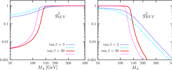
Figure 58: MSSM CP-even Higgs boson couplings to the weak gauge bosons as a function of $M_{A}$ and for two choices of $\tan\beta$, and for no mixing (darker colors) and maximal mixing (lighter colors). Figures from Ref. Djouadi .

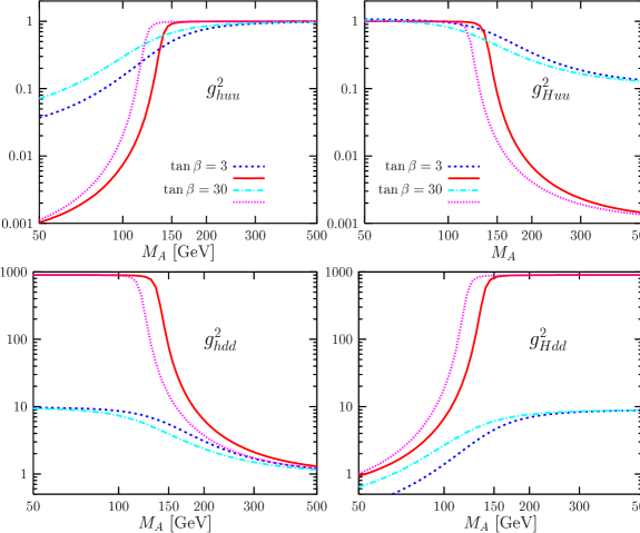
Figure 59: MSSM CP-even Higgs boson couplings to fermions as a function of $M_{A}$ and for two choices of $\tan\beta$, and for no mixing (darker colors) and maximal mixing (lighter colors). Figures from Ref. Djouadi .

These are the most salient features of the MSSM Higgs sector, sufficient to understand the bulk of MSSM Higgs phenomenology. For a more in-depth discussion, especially of why SUSY imposes these constraints, and for more detailed formulae, see Refs. Djouadi ; JackHowie_MSSM_H .

Now that we know the couplings, we can obtain cross sections for $h$ and $H$ production simply as correction factors to the SM channels of equal mass. There is no WBF or $W/Z$-associated pseudoscalar production, but there is both $gg\to A$ inclusive and top quark associated production, $t\bar{t}A$, which are easily obtained if one inserts the $\gamma_{5}$ factor into the loop derivation for $gg\to A$ Djouadi . The charged Higgs is a special case as there is no SM analogue; we’ll discuss this in Sec. IV.4 in the context of searches. For the moment, let’s examine the neutral states’ branching ratios, just to get an idea of how they behave. It’s easy to suffer plot overload about now, so don’t try to absorb every last detail; focus on the general behavior, which you already should be able to guess from the couplings plots.

Fig. 60 shows the BRs for the CP-even states $h$ and $H$, cut off at the mass plateaus. They’re basically what we would expect: both $h$ and $H$ behave like a SM Higgs of equal mass, except that the various couplings are dialed up or down. $M_{h}$ can never be above $\sim 145$ GeV, so it almost never has a significant BR to gauge bosons. Because the fermionic partial widths can be enhanced by a factor of $\tan^{2}\beta$, the rare modes like $\phi\to\gamma\gamma,gg$

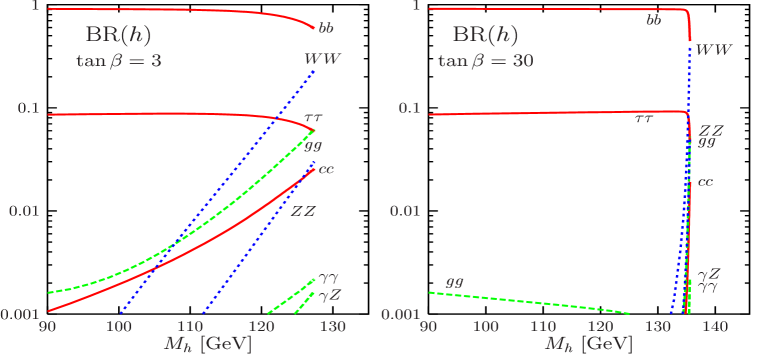
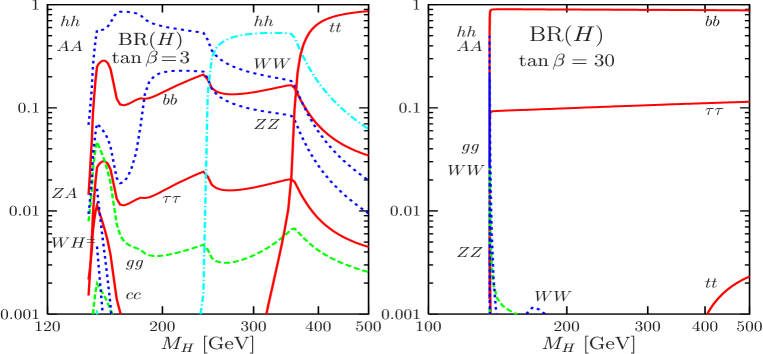
Figure 60: MSSM CP-even Higgs boson branching ratios as a function of $M_{A}$ for $\tan\beta=3,30$. Figures from Ref. Djouadi .

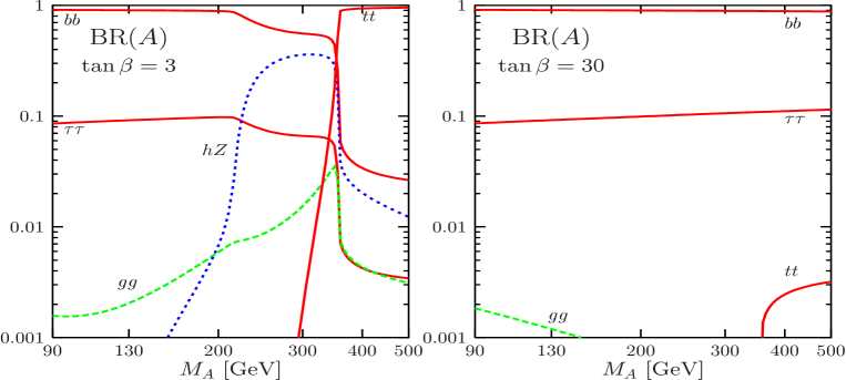
Figure 61: MSSM CP-odd Higgs boson branching ratios as a function of $M_{A}$ for two choices of $\tan\beta$. Figures from Ref. Djouadi .

tend to be suppressed (and the top quark loop can better cancel the $W$ loop for some parameter choices, suppressing the partial width). The only new features are $H\to hh,AA$ decays, possible for limited parameter choices but making for interesting additional channels.

The pseudoscalar BRs behave similarly, as shown in Fig. 61. The new feature here is at small $\tan\beta$, where decays $A\to hZ$ are possible. But otherwise $A$ prefers to decay $\sim 90\%$ to $b\bar{b}$ and $\sim 10\%$ to $\tau^{+}\tau^{-}$, unless it is heavy enough to produce top quark pairs. That dominates only at small $\tan\beta$ (large $\cot\beta$), where the up-type coupling dominates. At large $\tan\beta$, $b\bar{b}$ and $\tau^{+}\tau^{-}$ both still win by a considerable margin.

There are similar plots for $H^{\pm}$, but they’re not particularly enlightening as its decay patterns are drastically simpler: as far as phenomenology is concerned, it’s BR$\sim 1$ to $tb$ when kinematically accessible, $\tau\nu$ if lighter. For low $\tan\beta$ there is a rare BR to $hW^{\pm}$, but that is predicted to always be difficult to observe.

All Higgs bosons can decay to SUSY particle pairs if they’re light enough, but this is not a very common occurrence across parameter space (especially since so much of it is ruled out already by LEP SUSY searches), so we’ll bypass that discussion here.

IV.4 MSSM Higgs searches

For MSSM Higgs searches past, we start again with LEP. It didn’t find anything, but placed various limits. Let’s begin with the charged Higgs search, because it’s the simplest. This proceeded via $H^{+}H^{-}$ pair production (the only mechanism accessible at LEP) and decay to $\tau\nu$ or $cs$, as there was never kinematic room for $tb$. Thus, the search had three channels: dual taus, mixed tau plus hadronic decays, and an all-hadronic mode Okpara:2001ef . Because the production mechanism depends on only gauge-fixed couplings, the MSSM charged Higgs search is usually presented as a more general 2HDM search, with limits presented in the $M_{H^{\pm}}$ v. BR($H^{\pm}\to\tau^{\pm}\nu$) plane. Fig. 62 summarizes the obtained limits. To translate the general search limits to the MSSM Higgs sector inputs, recall Eq. 45, $M_{H^{\pm}}^{2}=M_{A}^{2}+M_{W}^{2}$. The difficulty of this search was the low ID efficiency for taus and charm quarks. Unfortunately, there is no final combined limit, but each of the collaborations has published final independent limits Heister:2002ev ; Abdallah:2003wd ; Achard:2003gt ; Horvath:2003kd . Watch the LEP-Higgs web page for updates LEP-HWG .

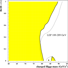
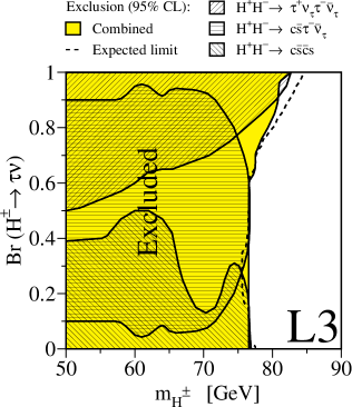
Figure 62: Left: LEP preliminary combined-experiment charged Higgs search $95\%$CL limits (2001), from Ref. unknown:2001xy . Right: L3 published limits from 2003, illustrating where each of the three decay channels discussed in the text contributes to the overall limit Achard:2003gt . There is no final LEP combined limit, but judging from each of the individual limits Heister:2002ev ; Abdallah:2003wd ; Achard:2003gt ; Horvath:2003kd , it does not change significantly from the preliminary results.

The basic neutral Higgs boson search channels are exactly the same as in the SM for each of $h$ and $H$, to which we add $e^{+}e^{-}\to Z^{*}\to hA/HA$ production via the additional couplings of Table 5. Each of the four LEP collaborations presented a multitude of MSSM $h/H/A$ search limits, and there are combined LEP results with CP-conservation Schael:2006cr and CP-violation (CPX) Schael:2006cr ; Bechtle:2006iw . However, one should be somewhat wary of what precisely is presented. The results are usually shown as shaded exclusion blobs in either $M_{A}$-$\tan\beta$ space (for a very specific set of additional assumptions) or $M_{h_{i}}$-$\tan\beta$ space, also given some assumptions. There are literally dozens of pages of exclusion plots, depending on what one chooses for the mixing parameter $X_{t}$, top quark mass (recall the strong $M_{h}$ dependence on $m_{t}$), stop masses, $\mu$, and so on. This is far too much to show here, because the exclusion contours change so much from assumption to assumption – it’s impossible even to select a representative sample without misleading the uninitiated. See e.g. Ref. Sopczak:2006vn .

The curious student should flip through the plots in Refs. Schael:2006cr ; Sopczak:2006vn simply to get a feel for how wild this variation is. Observe how much the contours change depending on the top quark mass – it is obviously still fairly poorly measured, as far as fits to supersymmetry go. Note also that the plots are always logarithmic in $\tan\beta$, which compresses the unexcluded large-$\tan\beta$ region, making it appear that parameter space is vastly ruled out in many cases. This simply isn’t true. Finally, I should comment that the “theoretically inaccessible” disallowed blobs are even more grossly misleading. All one has to do is move the stop masses up slightly and these retreat dramatically. Perhaps a more logical approach is the model-independent $h/H/A$ search of OPAL Abbiendi:2004gn .

MSSM Higgs Searches at LHC are also mostly variants on the SM search channels, the exceptions being charged Higgses, rare (SUSY or Higgs pair) decay modes, and one new production channel, $b\bar{b}\phi$, which is important at large $\tan\beta$ where the coupling is enhanced to top-quark Yukawa strength. $t\bar{t}\phi$ rates tend to be about the same as the SM for equal mass, or slightly suppressed. WBF $h$ or $H$ rates can only be suppressed relative to the SM, due to the appearance of $\sin^{2}(\beta-\alpha)$ or $\cos^{2}(\beta-\alpha)$, respectively. Inclusive rates can change rather dramatically, however, because the $b$ loop can be extremely important. Fig. 63 shows the cross sections for $gg\to\phi$ as a function of the physical masses, for small and large $\tan\beta$. These may be compared with the SM cross sections of Fig. 16.

Let’s concentrate on the WBF modes, however, as they turn out to be the most interesting. Recall the plateau behavior of $h$ and $H$ masses as a function of $M_{A}$ (cf. Fig. 57), and simultaneously the $h$ and $H$ gauge coupling behavior (cf. Fig. 58). The astute student will realize that this implies that WBF Higgs production in an accessible mass region probably always occurs at a good rate, somewhat suppressed but never much so. Fig. 64 summarizes some of this previous information and goes on to show the cross section times BR to tau pairs (in the two accessible tau decay modes), also as a function of $M_{A}$ Plehn:1999nw . Indeed, eyeballing the upper and lower rows, it appears that between $h$ and $H$, there’s always a signal in WBF. It may be slightly suppressed, but we know from SM WBF Higgs studies (cf. Sec. II.3.4) that since so little data is required to make an observation, the signal could be suppressed by a factor of several and be detectable. The reason is that in the MSSM the $h$ and $H$ plateau mass ranges are in the “good” region of WBF Higgs observability. Actually, quite a large mass region is observable, but if the MSSM predicted Higgs masses closer to the $Z$ pole, there could be trouble (but LEP would already have discovered such a Higgs).

This bit of luck forms the basis of the MSSM Higgs No-Lose Theorem: at least one of the CP-even Higgs states, $h$ or $H$, is guaranteed to be observable in WBF at LHC Plehn:1999nw ; Plehn:1999xi . The original parton-level studies have since been confirmed with full ATLAS detector simulation, and actually improved Schumacher:2004da . The parton-level coverage plots shown in Fig. 65, however, are simpler to grasp. Very little data would be required for discovery, and for some $M_{A}$ it would be possible to observe both $h$ and $H$ simultaneously.

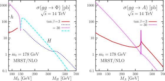
Figure 63: Gluon fusion MSSM Higgs production cross sections at LHC for the CP-even states $h$ and $H$ (left) and the pseudoscalar $A$ (right), for two values of $\tan\beta$. Figures from Ref. Djouadi .

Figure 64: From left to right, each plot as a function of $M_{A}$: $h/H$ mass, gauge coupling suppression factor squared, WBF cross section times BR to taus to the lepton-hadron final state, and the same for the dual lepton mode. The upper (lower) row is for $h$($H$). Fig. from Ref. Plehn:1999xi .

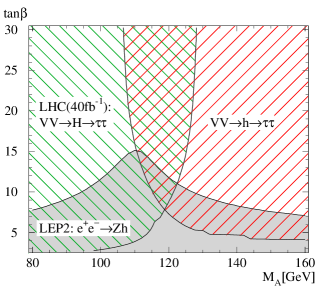
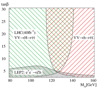
Figure 65: MSSM parameter space coverage of WBF $h/H\to\tau^{+}\tau^{-}$ for the no-mixing ($A_{t}=0$, left) and maximal mixing ($X_{t}=\sqrt{6}\,M_{SUSY}$, right) cases Plehn:1999nw .

One caveat: the final state $\tau^{+}\tau^{-}$ is not always accessible! It’s possible to zero out the MSSM down-type fermion coupling at tree level – an interesting exercise for the student. If this happens, $h/H\to\gamma\gamma$ and $h/H\to W^{+}W^{-}$ are “large” partial widths, so their BRs take up the coverage slack Plehn:1999nw ; Schumacher:2004da , saving the No-Lose Theorem. There’s been some work on an NMSSM No-Lose Theorem Ellwanger:2001iw ; Ellwanger:2003jt ; Ellwanger:2005uu ; Moretti:2006hq , which extends the Higgs sector by a complex singlet HHG . The outlook for LHC is promising, but not obviously rock-solid.

The No-Lose Theorem is great for the CP-even states, but what about the other Higgses? I’ll gloss over the bulk of searches, since they’re mostly variants on the SM ones, and move on to the special case of heavy $H/A$ (towards decoupling) and this new channel $b\bar{b}\phi$. The Feynman diagrams appear in Fig. 66. Recall that $H$ has a $\tan\beta$ enhancement to down-type quarks in the decoupling region, and $A$ always has this enhancement. We already know that means that $H$ and $A$ prefer to decay $90\%$ of the time to $b\bar{b}$ and $10\%$ to $\tau^{+}\tau^{-}$, but it would be impossible to observe either of those final states in inclusive production, and WBF production is zilch for $H$ in the decoupling region. However, the LHC being essentially a gluon collider, the initial state can create high-energy $b$ pairs, which can then Brem a Higgs, either $H$ or $A$, which are essentially degenerate (but do not interfere due to the $\gamma_{5}$ coupling). Since the $b$ jets are produced at high-$p_{T}$, the $H/A$ must recoil against them, so it also produced with a transverse boost. It’s decay products are then not back-to-back, allowing for tau pair reconstruction; $H/A\to\mu^{+}\mu^{-}$ may also be used, but is a rare mode. The final state is then $b\bar{b}\tau^{+}\tau^{-}$ (or $b\bar{b}\mu^{+}\mu^{-}$), which is taggable and distinguishable from mixed QCD-EW backgrounds because the tau pair invariant mass is in the several-hundred GeV region.

Fig. 67 shows the cross section times BR to tau pairs for 300 GeV Higgs bosons as a function of $\tan\beta$, and also the CMS expected discovery reach for various final states in tau or muon pairs, with only 30 fb^-1 of luminosity, or about 1/10 of the total LHC data expected. Coverage is not complete, because this mode doesn’t produce enough rate at low $\tan\beta$ where there is little coupling enhancement, but is still a significant search tool. The mass resolution achievable for $H$ and $A$ using taus in this mode is even pretty good, on the order of a couple tens of GeV, possibly better. Of course, if the decay to muons is accessible (at very large $\tan\beta$, then mass resolution would be on the order of a GeV.

This would determine $M_{A}$ quite well, good enough for comparison with theory (at least at first), but what about the other major Higgs parameter, $\tan\beta$? The $b\bar{b}\phi$ production rate is directly proportional to $\tan^{2}\beta$, so we can measure it using the overall rate, with the mild (but not rock solid) assumption that the ratio of $b\bar{b}$ and $\tau^{+}\tau^{-}$ BRs is the ratio of the $b$ and $\tau$ squared masses, i.e. that BR($H/A\to\tau^{+}\tau^{-}$) $\sim 10\%$ Kinnunen:2004ji . The major sources of uncertainty are this assumption, the machine luminosity uncertainty of $5-10\%$, PDF uncertainties of probably about $5\%$, and higher-order QCD corrections to the production process of probably about $20\%$ Dittmaier:2003ej ; Dawson:2005vi .

Fig. 68 shows the CMS expected uncertainty on $\tan\beta$ using this method, as a function of $M_{A}$ and for 30 or 60 fb^-1 of data. In general, $10-20\%$ appears achieveable. This is not spectacular, but would be a significant first step toward sorting out the new Higgs sector and presumably comparing to other SUSY discovery measurements. Clearly the higher-order QCD uncertainties dominate, which could probably be improved with better theoretical calculations over the next decade. This will be done if heavy Higgses are discovered.

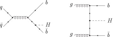
Figure 66: Feynman diagrams for $gg\to b\bar{b}\phi$ production at LHC.

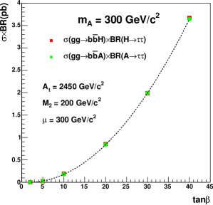
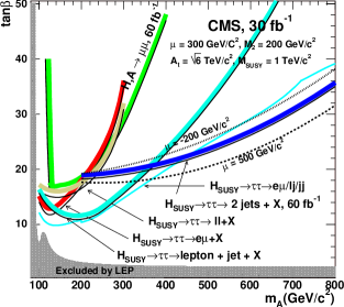
Figure 67: Left: $b\bar{b}\phi$ production cross section at LHC times the BR to tau pairs, as a function of $\tan\beta$ for $M_{A}=300$ GeV. Right: expected CMS reach using only 30 fb^-1 of data for $b\bar{b}H/A\to\tau^{+}\tau^{-},\mu^{+}\mu^{-}$ as a function of $M_{A}$. Figures from Ref. Kinnunen:2004ji .

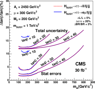
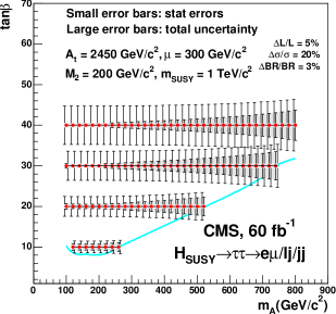
Figure 68: CMS expected precision on $\tan\beta$ at LHC using $b\bar{b}\phi$ production as described in the text. Figures from Ref. Kinnunen:2004ji .

Now, what about charged Higgs discovery? We know nothing about its phenomenology, because there is no SM analogue. All we do know is the very important fact that, despite everything else we may see at Tevatron or LHC, the only way to prove the existence of two Higgs doublets is to directly observe the charged Higgs states. I cannot emphasize this enough. For all we know, an extra neutral state might simply be the residue of an extra Higgs singlet; there could be more to the flavor sector that confuses us when we try to measure Yukawa couplings or $\tan\beta$. Thus, observing the $H^{\pm}$ states would be a huge qualitative step toward understanding what the Higgs sector is. How would this proceed experimentally?

Figure 69: Feynman diagrams for charged Higgs production at hadron colliders. The short line breaking the $b$ quark propagator represents how the process may also be regarded as initiated by a $b$ parton in the proton, rather than from gluon splitting to a $b$ quark pair.

At Tevatron there is very little energy available for direct charged Higgs production, since it must be produced in association with a top quark (large coupling), as shown in the Feynman diagrams of Fig. 69. However, if $M_{H^{\pm}}$ is small enough, the top quark can decay to $bH^{\pm}$ followed by $H^{\pm}\to\tau\nu$ if $\tan\beta>1$, and equally to $bc$ and $cs$ if $\tan\beta<1$; if $M_{H^{\pm}}\gtrsim 120$ GeV, then the BR to $W^{\pm}b\bar{b}$ via a top quark loop becomes significant. Fig. 70 shows the $t\to bH^{\pm}$ BR as a function of $M_{H^{\pm}}$ for a few select $\tan\beta$, and as a function of $\tan\beta$ for $M_{H^{\pm}}=120$ GeV. At low $\tan\beta$, the partial width is driven mainly by the top quark Yukawa, while at large $\tan\beta$ it’s primarily the bottom quark. Weakness of both Yukawas in the intermediate-$\tan\beta$ regime results in a comparatively reduced top quark partial width (recall Eqs. (41,42)). For fixed $M_{H^{\pm}}$, the partial width is symmetric in $\log(\tan\beta)$ about a minimum at $\tan\beta=\sqrt{m_{t}/m_{b}}$. Charged Higgs decays to $hW^{\pm}$ or $AW^{\pm}$ are generally disallowed in the MSSM from LEP mass limits on $h$ and $A$.

The Tevatron search proceeds both as appearance (i.e. looking directly for $H^{\pm}$ in the top quark sample) and disappearance, or missing rate for top quark to $bW^{\pm}$. Fig. 71 goes on to show the expected $95\%$ CL limits in the $M_{H^{\pm}}-\tan\beta$ plane that Tevatron Run I achieved, and Run II might reach depending on how much data it ultimately records. The very slight change between 2 and 10 fb^-1 reveals that the experiments there are statistics-limited, but not by a great margin.

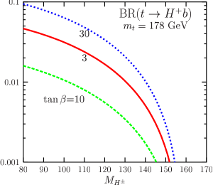
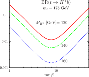
Figure 70: Branching ratio for top quark to bottom quark plus charged Higgs boson, as a function of $M_{H^{\pm}}$ for a few select values of $\tan\beta$ (left) and as a function of $\tan\beta$ for $M_{H^{\pm}}=120$ GeV (right). Figures from Ref. Djouadi .

Figure 71: Tevatron Run I $95\%$ CL charged Higgs mass limits (double hatched lines) as a function of $\tan\beta$ from searches for top quark decays to bottom quark plus charged Higgs, and expected limits achievable in Run II (single hatched lines for 2 fb^-1, unhatched curves for 10 fb^-1). Fig. from Ref. Chakraborty:2003iw .

LHC will search for $tH^{\pm}$ direct production (Fig. 69), covering the mass range $M_{H^{\pm}}>m_{t}$. Due to nasty QCD backgrounds, the $tb$ decay will be inaccessible Assamagan:2004mu , leaving $\tau\nu$ with BR$\sim 10\%$. This is very difficult due to a subtlety of tau decays. Left-handed taus decay to soft leptons Hagiwara:1989fn . Since neutrinos are left-handed, helicity conservation in scalar decay means all taus are as well. We need a lepton to trigger the event, and it must come from $H^{\pm}$ instead of $t$, so that there is only one source of missing transverse momentum and we can fully reconstruct $t$, and $H^{\pm}$ transversely. Only a small fraction of the small rate could pass the necessary detector kinematic cuts to be recorded. This limits the search to large $\tan\beta$ or small $M_{H^{\pm}}$, where the production rate is largest. Fig. 72 shows ATLAS’s expected transverse mass distributions for a fairly light and a heavy $H^{\pm}$.

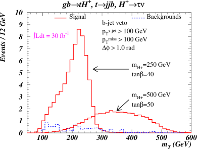
Figure 72: Expected transverse mass distributions for light and heavy $H^{\pm}\to\tau\nu$ at ATLAS Assamagan:2002ne .

Finally, we come to the overall picture of MSSM Higgs phenomenology at LHC. Primarily we’re concerned with discovering all the states, but especially the charged Higgs as it’s the key to confirming the existence of two Higgs doublets. That turns out to be extraordinarily difficult due to a combination of factors, from overwhelming QCD backgrounds to characteristics of left-handed tau decays. Fig. 73 summarizes the reach for $h$, $H$, $A$ and $H^{\pm}$ Gianotti:2002xx . It’s reassuring that the No-Lose Theorem holds and we’re guaranteed to find at least one of the CP-even states, $h$ or $H$. However, moderate $\tan\beta$ and the decoupling limit (large $M_{A}$) both present significant gaps in coverage to observe any of the additional states. This is especially more apparent once one realizes that the region below the solid black curve is already excluded by LEP, so those LHC access regions don’t matter. The figure is from 2001 and needs updating – some significant positive changes exist – but the general picture remains.

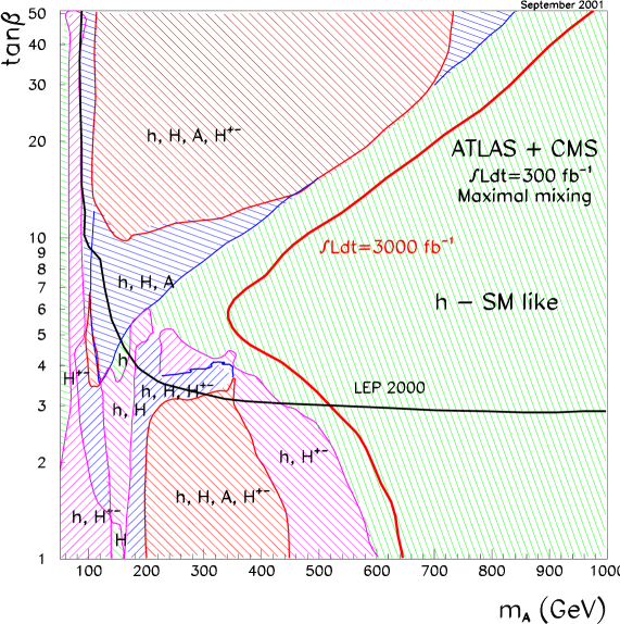
Figure 73: Summary of MSSM Higgs boson discovery reaches at LHC (and extended to SLHC via the solid red line), combining ATLAS and CMS, in the $\tan\beta-M_{A}$ plane in the maximal mixing scenario. The reach is defined as $5\sigma$ discovery in at least one production and decay channel. Below the solid black curve is the region excluded by LEP. Figure from Ref. Gianotti:2002xx .

IV.5 MSSM Higgs potential

I’ve touched on the bits of Higgs gauge and Yukawa couplings in the MSSM that are qualitatively different that the SM: $M_{A}$ and $\tan\beta$. But we should look at self-couplings more closely, because in a general 2HDM (or the subset MSSM) they are radically different. First, because there are more Higgs bosons, there are more self-couplings – six for the neutral states alone, to be precise: $\lambda_{hhh}$, $\lambda_{Hhh}$, $\lambda_{HHh}$, $\lambda_{HHH}$, $\lambda_{hAA}$, $\lambda_{HAA}$. In the MSSM these are all equal to $M_{Z}^{2}/v$ times various mixing angles (which aren’t particularly enlightening so I don’t show them) plus additional shifts from top quark Yukawa loop corrections. That is, they are all (mostly) gauge parameters. However, in the large-$M_{A}$ decoupling limit which recovers the SM, $\lambda_{hhh}\to\lambda_{\rm SM}$.

If we discover SUSY, we’d start by assuming it’s the MSSM. To measure the MSSM potential in that case, we’d have to observe at least six different Higgs pair production modes to measure the six self-couplings. (Note that I’m leaving out the possible self-couplings involving charged Higgses.) Inclusive Higgs pair production looks generally like it does in the SM, $gg\to\phi_{1}\phi_{2}$ via triangle and box loop diagrams as shown in Fig. 74, but the $b$ quark loops become important and must be included.

Unfortunately, the box diagram totally swamps the one containing the self-coupling we care about by a factor $\tan^{2}\beta$, and in any case backgrounds from $H/Ab\bar{b}$ production appear to be overwhelming Baur:2003gp : very generally, LHC would not obtain any $\lambda$ measurements at all. The one very limited exception is that LHC could clearly observe Higgs pair production if it came from resonant heavy Higgs decay, $H/A\to hh$. An example peak is shown in Fig. 75. However, this would measure only a BR, at best, not an absolute coupling. Sadly, exactly the same situation exists for Higgs pairs at a future ILC Djouadi:1999gv .

Figure 74: Feynman diagrams for Higgs pair production in a 2HDM like the MSSM. The loops include both top and bottom quarks, and there are six possible processes (see text).

Figure 75: Resonant MSSM Higgs pair production at LHC and decay to $b\bar{b}\gamma\gamma$ final states Baur:2003gp .

V Conclusions

The purpose of these lectures has not been to provide exhaustive coverage of all aspects of collider Higgs phenomenology. Rather, it’s a solid introduction, focusing on the basics. This includes SM production and decay, mostly at LHC, where we’re confident we could discovery a SM-like Higgs, and many non-SM-like variants. I focused on the most important channels which guarantee discovery, and especially in weak boson fusion (WBF) as those are the most powerful (best $S/B$, distinctive) search channels, covering the broadest range of Higgs mass. I emphasized that our understanding of LHC Higgs physics has changed dramatically from the days of the ATLAS TDR, for example, which is now quite obsolete. However, ATLAS has produced a plethora of Notes and summaries of Notes to cover the changes, and CMS published a fresh TDR CMS_TDR in 2006 which covers the changes as well.

We now understand the LHC to be such a spectacular Higgs factory that not only can it discover any mass of SM-like Higgs boson, it can also do an impressive job of measuring all its quantum properties. Granted, Higgs couplings measurements won’t be precision-level if the Higgs is light, as expected from EW precision data, but they would nonetheless be absolute couplings measurements. The LHC can even make significant steps toward measuring the SM Higgs potential, at least the Higgs trilinear self-coupling, although depending on $M_{h}$ it may require precision gauge and Yukawa couplings input from a future $e^{+}e^{-}$ collider (an ILC) to control the major systematic uncertainties. I also highlighted where an ILC could make improvements to the LHC’s measurements, and where it would be vital to filling in gaps in LHC results.

The final third of the lectures discussed BSM Higgs sectors, but only the 2HDM MSSM Higgs sector in any detail. Many SM Higgs sector extensions are rather simple variants on SM phenomenology, involving factorizable changes in production and decay rates (couplings), mostly arising from mixing angles. This is not general, however, and there are plenty of “exotic” models – Higgs triplets, for example – which would be qualitatively different, but therefore simultaneously distinctive. The popular focus on the MSSM 2HDM is because of several other outstanding questions in particle physics, like dark matter or the theoretical dirty laundry of the SM Higgs sector, which strongly motivate the other new physics.

Students who wish to engage in Higgs phenomenology research should definitely take the time to expand their scope beyond the SM and the MSSM. Other extensions are equally well-motivated, such as Little Higgs, not to mention strong dynamics. But the two well-studied basic models I covered here give one a strong foundation for other BSM Higgs phenomenology by analogy. Happy Higgs hunting!