The Stueckelberg $Z^{\prime}$ Extension with Kinetic Mixing
and Milli-Charged Dark Matter from the Hidden Sector

Abstract

An analysis is given of the Stueckelberg extension of the Standard Model with a hidden sector gauge group $U(1)_{X}$ where the mass growth for the extra gauge boson occurs via the Stueckelberg mechanism, and where the kinetic mixing in the $U(1)_{X}\times U(1)_{Y}$ sector is included. Such a kinetic mixing is generic in a broad class of supergravity and string models. We carry out a detailed global fit of the model with the precision LEP data on and off the $Z$ pole, with $\chi^{2}$ within 1% of the $\chi^{2}$ of the Standard Model fit. Further, it is shown that in the absence of matter in the hidden sector, there is a single effective parameter that controls the deviations from the Standard Model predictions, and the dependence on the kinetic mixing emerges only when matter in the hidden sector is included. An analysis is also given of milli-charged dark matter arising from the hidden sector, where it is shown that such dark matter from the Stueckelberg extension can satisfy WMAP-3 data while allowing for a sharp $Z^{\prime}$ resonance which can be detected at the Tevatron and at the LHC via a dilepton signal generated by the Drell-Yan process.

I Introduction

Recent works on the Stueckelberg extension of the SM kn1 (StSM) and of the MSSM kn2 ; kn3 (StMSSM), have shown consistency with the LEP data while allowing for the possibility of a narrow resonance which could lie as low as just above the $Z$ mass kn1 ; kn2 ; kn3 ; fln1 ; fln2 . Similar phenomena regarding a narrow resonance are seen in other classes of models such as those based on universal extra dimensions UED , models with a shadow sector holdom ; Kumar:2006gm ; Chang:2006fp , and in the models considered in Ref. Ferroglia:2006mj . The possibility of a narrow graviton resonance also arises in the RS model Randall:1999ee ; Davoudiasl:1999jd . Thus the study of narrow resonances is a topic of significant interest. In this work we focus on the Stueckelberg extensions further. Such models may be a field theory realization of string models arising from orientifolds ghi ; Ibanez:2001nd ; Anastasopoulos:2006cz ; recent_ST ; Anastasopoulos:2007qm and their discovery could be harbingers of a new regime of physics altogether. The supersymmetric Stueckelberg extensions have the possibility of generating a new type of neutral Majorana fermion which is massive and extra-weakly interacting, and with R parity conservation, a candidate for cold dark matter Feldman:2006wd . Indeed a detailed analysis shows that the relic density in such models is consistent with the three year WMAP data Spergel:2006hy . Additionally, the Stueckelberg extensions give rise to milli-charges for matter residing in the hidden sectorkn1 ; kn3 . A recent analysis kctc indicates that such matter can annihilate in sufficient amounts to satisfy the relic density constraints from WMAP-3 for a broad $Z^{\prime}$ resonance.

The main focus of this work is an extension of the class of models considered in Refs. kn1 ; kn2 ; kn3 ; fln1 ; fln2 by including kinetic mixing between the two Abelian $U(1)$ gauge fields. Specifically we consider the extended electroweak sector with the gauge groups $SU(2)_{L}\times U(1)_{Y}\times U(1)_{X}$ where the Stueckelberg mechanism along with the spontaneous breaking in the Higgs sector generates the vector boson mass, and a mixing in the gauge kinetic energy of the $U(1)_{X}\times U(1)_{Y}$ sector is included. Such kinetic mixings can arise in a variety of ways bkm ; dkm and enter prominently in models of the type considered in Refs. Kumar:2006gm ; Chang:2006fp . The model considered here encompasses the models of Refs.kn1 ; kn2 ; kn3 ; fln1 ; fln2 which can be obtained in certain limits of the model discussed here. Inclusion of the kinetic mixing in the Stueckelberg extension enhances significantly the parameter space where new physics can exist consistent with the stringent LEP, Tevatron, and WMAP constraints. This parameter space includes the possibility of a narrow $Z^{\prime}$ resonance very distinct from the $Z^{\prime}$ of the conventional models u1 ; d1 ; PhemZp .

The outline of the rest of the paper is as follows: In Sec.(II) we give a description of the Stueckelberg extension with kinetic mixing in the $U(1)_{X}\times U(1)_{Y}$ sector. In Sec.(III) we give a detailed numerical analysis of the electroweak constraints from LEPI and LEPII. In Sec.(IV) an analysis of milli-charged dark matter that arises from the hidden sector is given. Conclusions are given in Sec.(V). Appendices contain several mathematical details, including an analysis regarding the origin of milli-charged matter.

II The Stueckelberg $Z^{\prime}$ Extension with Kinetic Mixing

In this section we discuss the $U(1)_{X}$ Stueckelberg stueck extension of the Standard Model (SM) with gauge kinetic mixing (StkSM). We assume that the quarks, leptons and the Higgs field of the SM do not carry $U(1)_{X}$ quantum numbers, and the fields in the hidden sector do not carry quantum numbers of the SM gauge group. Thus the $U(1)_{X}$ sector is hidden except for the $U(1)_{X}\times U(1)_{Y}$ mixings in the gauge vector boson sector as given by the effective Lagrangian

$$\mathcal{L}_{\rm StkSM} = \mathcal{L}_{\rm SM}+\Delta\mathcal{L},$$

$$\Delta\mathcal{L} \supset -\frac{1}{4}C_{\mu\nu}C^{\mu\nu}-\frac{\delta}{2}C_{\mu\nu}B^{\mu\nu}$$

$$-\frac{1}{2}(\partial_{\mu}\sigma+M_{1}C_{\mu}+M_{2}B_{\mu})^{2}+g_{X}J^{\mu}_{X}C_{\mu}.$$

Here $B_{\mu}$ is the $U(1)_{Y}$ gauge field, $C_{\mu}$ is the $U(1)_{X}$ gauge field with coupling strength $g_{X}$ to hidden matter through the source $J_{X}$, $\sigma$ is the axion, $M_{1}$ and $M_{2}$ are mass parameters, and $\delta$ is the kinetic mixing parameter. The $\sigma$ field is charged under both $U(1)_{X}$ and $U(1)_{Y}$ and the Lagrangian of Eq. (1) is invariant under the $U(1)_{X}\times U(1)_{Y}$ gauge transformations

$$\delta B_{\mu}=\partial_{\mu}\lambda_{X},~{}\delta C_{\mu}=0,~{}~{}\delta\sigma=-M_{2}\lambda_{X}$$

$$\delta B_{\mu}=0,~{}\delta C_{\mu}=\partial_{\mu}\lambda_{Y},~{}\delta\sigma=-M_{1}\lambda_{Y}.$$ (2)

The above model has a non-diagonal kinetic mixing matrix ($\mathcal{K}$) and a non-diagonal mass matrix (${M}^{2}_{\rm St}$) and in the unitary gauge kn1 in the basis $V^{T}=(C,B,A^{3})$

$$\mathcal{K}=\left[\matrix{1&\delta&0\cr\delta&1&0\cr 0&0&1}\right],$$ (3)

$${M}_{{\rm St}}^{2}=\left[\matrix{M_{1}^{2}&M_{1}M_{2}&0\cr M_{1}M_{2}&M_{2}^{2}+\frac{1}{4}v^{2}g_{Y}^{2}&-\frac{1}{4}v^{2}g_{2}g_{Y}\cr 0&-\frac{1}{4}v^{2}g_{2}g_{Y}&\frac{1}{4}v^{2}g_{2}^{2}}\right].$$ (4)

A simultaneous diagonalization of the kinetic energy and of the mass matrix can be obtained by a transformation $T=KR$, which is a combination of a $GL(3)$ transformation ($K$) and an orthogonal transformation ($R$). This allows one to work in the diagonal basis, denoted by $E$ where $E^{T}=(Z^{\prime},Z,A_{\gamma})$, through the transformation $V=(KR)E$, where the matrix $K$ which diagonalizes the kinetic terms has the form

$$K=\left[\matrix{C_{\delta}&0&0\cr-S_{\delta}&1&0\cr 0&0&1}\right],\hskip 4.26773ptC_{\delta}=\frac{1}{\sqrt{1-\delta^{2}}},\hskip 4.26773ptS_{\delta}=\delta C_{\delta}.$$ (5)

The matrix $R$ is then defined by the diagonalization of the mass matrix

$$M^{2}_{D}=R^{T}(K^{T}M^{2}_{\rm St}K)R.$$ (6)

The model of Eq.(1) involves three parameters: $M_{1},M_{2},\delta$ or alternately $M_{1},\epsilon,\delta$ where $\epsilon=M_{2}/M_{1}$. Expressing the transformation $T=KR$ in terms of the matrix elements, one has

$$\begin{array}[]{l}T_{1j}=C_{\delta}R_{1j},\\ T_{2j}=R_{2j}-S_{\delta}R_{1j},\\ T_{3j}=R_{3j}.\end{array}$$

The neutral current interaction with the visible sector fermions is given by

$${\mathcal{L}}_{NC}=-\frac{1}{i}\sum\limits_{f}[{\bar{f}}_{L}D_{\mu}\gamma^{\mu}f_{L}+(L\rightarrow R)],$$ (7)

where $D_{\mu}$ is the covariant derivative with respect to $SU(2)_{L}\times U(1)_{Y}\times U(1)_{X}$ gauge group except that, as mentioned in the beginning, we assume that the visible sector matter, i.e., quarks, leptons and the Higgs, are not charged under $U(1)_{X}$. Thus the covariant derivative includes only the $SU(2)_{L}$ gauge coupling $g_{2}$ and $U(1)_{Y}$ gauge coupling $g_{Y}$. The diagonalization also leads to the following relation for the electronic charge

$$\frac{1}{e^{2}}=\frac{1}{g_{2}^{2}}+\frac{1-2\epsilon\delta+\epsilon^{2}}{g_{Y}^{2}}.$$ (8)

Thus $g_{Y}$ is related to $g_{Y}^{SM}$ by

$$g_{Y}=\gamma\sqrt{1+\epsilon^{2}-2\delta\epsilon},\hskip 14.22636pt\gamma\equiv g^{SM}_{Y},$$ (9)

and one may write the neutral current interaction so that

$${\cal L}_{NC}=\frac{\sqrt{g^{2}_{2}+\gamma^{2}}}{2}\bar{f}\gamma^{\mu}\left[(v^{\prime}_{f}-\gamma_{5}a^{\prime}_{f})Z^{\prime}_{\mu}+(v_{f}-\gamma_{5}a_{f})Z_{\mu}\right]f+e\bar{f}\gamma^{\mu}Q_{f}A_{\mu}f,$$ (10)

where

$$\begin{array}[]{l}v_{f}=\frac{1}{\sqrt{g^{2}_{2}+\gamma^{2}}}[(g_{2}T_{32}-g_{Y}T_{22})T^{3}_{f}+2g_{Y}T_{22}Q_{f}],\\ a_{f}=\frac{1}{\sqrt{g^{2}_{2}+\gamma^{2}}}[(g_{2}T_{32}-g_{Y}T_{22})T^{3}_{f}],\\ v^{\prime}_{f}=\frac{1}{\sqrt{g^{2}_{2}+\gamma^{2}}}[(g_{2}T_{31}-g_{Y}T_{21})T^{3}_{f}+2g_{Y}T_{21}Q_{f}],\\ a^{\prime}_{f}=\frac{1}{\sqrt{g^{2}_{2}+\gamma^{2}}}[(g_{2}T_{31}-g_{Y}T_{21})T^{3}_{f}],\\ \end{array}$$ (11)

and where, as usual, $Q_{f}=T^{3}_{f}+Y_{f}/2$. We note that the mass and kinetic mixing parameters enter not only through $T_{ij}$ but also through $g_{Y}$ via the constraint of Eq.(8).

III Constraints from
electroweak data

We discuss now the constraints on the model with both mass mixing and kinetic mixing from the precision electroweak data. We start by assuming that the hidden sector does not contain matter, and the case when matter is included in the hidden sector is discussed in Sec.(IV) and in Appendix B. To obtain the allowed range of $\epsilon$ and $\delta$, we follow the same approach as in Ref. Nath:1999fs ; fln1 ; fln2 . The first constraint comes from the comparison of the one sigma error in the prediction of the $Z$ boson mass in the Standard Model and a comparison of this result with experiment, leads to an error corridor, $\delta M_{Z}\sim 37$ MeV, where one can accommodate new physics. However, the more stringent constraint comes from fits to the high precision LEP data on the branching ratios of the $Z$ decay and from the various asymmetries at the $Z$ pole, when one demands that the $\chi^{2}$ fits of StkSM are within 1% of that of the Standard Model. We will refer to this as the LEPI 1% constraint in the rest of the paper. Details of the method employed for the electroweak fits can be found in the analysis of Ref. fln1 ; fln2 , and here we present just the results in the extended model with kinetic mixing.

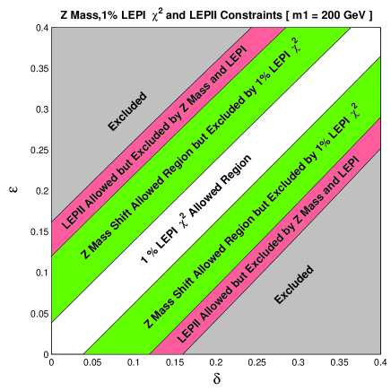
Figure 1: An analysis of $\chi^{2}$ in StkSM model in the $\epsilon-\delta$ plane. The center white region is where $\chi^{2}$ of the StkSM model is within 1% of the SM fits. Along the line $\epsilon=\delta$ the $Z^{\prime}$ decouples and the model gives the same $\chi^{2}$ fit to data as in the SM (see also Appendix A).

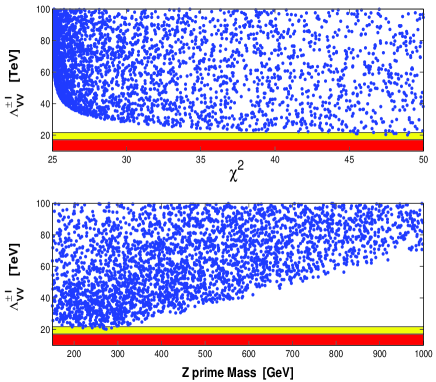
Figure 2: The plots give an analysis of the LEPII constraint. The upper plot, which has a $Z^{\prime}$ mass range of $.2-1$ TeV, shows the relevant LEPII contact interaction parameter $\Lambda^{\pm l}_{VV}$ as a function of $\chi^{2}$ for the 19 observable of Table(1), where a $\chi^{2}\sim$ 25 is the SM fit as given in Table(1), and where the (yellow,red) shaded regions correspond to $\Lambda^{\pm l}_{VV}$ = (21.7, 17.1) TeV Leptwo . The lower plot for $\chi^{2}$ in the range (25-50) gives $\Lambda^{\pm l}_{VV}$ as a function of the $Z$ prime mass.

Table 1 gives a fit to the LEP data for a specific point in the Stueckelberg parameter space with $\epsilon=.06$, $\delta=.03$, and $M_{Z^{\prime}}\approx M_{1}=200$ GeV. In the analysis we have taken into account the constraint between $g_{Y}$ and $g_{Y}^{SM}$ and the inclusion of this constraint improves the electroweak fits over that of previous analyses for the case $\delta=0$ fln1 ; fln2 . Thus the analysis of Table 1 shows that in the StkSM one finds $\chi^{2}$ fits which are at the same level as in the SM. An analysis of $\chi^{2}$ in the LEPI fits in the $\epsilon-\delta$ parameter space is given in Fig.(1). Specifically Fig.(1) shows that a large region of the parameter space can satisfy the LEPI 1% constraint. A striking aspect of the analysis of Fig.(1) is that this constraint is satisfied even though $\epsilon$ and $\delta$ can get significantly large, as long as $(\epsilon-\delta)$ is small. The physics of this is explained in Appendix A where it is shown that in the absence of matter in the hidden sector, there is only one effective parameter, $\bar{\epsilon}$, that enters the analysis of electroweak physics.

Table 1: Fits to 19 $Z$ pole observables. Column 2 is given by the PDG pdg , while the data in column 3 is from the SM Fit of the LEP EWWG :2005em . The column labeled St Fit is an analysis for the input $\epsilon=0.06$, $\delta=0.03$, and $M_{1}=200$ GeV. In the last column PULL is defined by $(\rm Experiment-\rm FIT)/\Delta$, and $\chi^{2}=\sum{\small{\rm{PULL}}^{2}}$.

Quantity	Experiment $\pm\Delta$	LEP FIT	St FIT	LEP PULL	St PULL
$\Gamma_{Z}$ [GeV]	2.4952 $\pm$ 0.0023	2.4956	2.4956	-0.17	-0.17
$\sigma_{\rm had}$ [nb]	41.541 $\pm$ 0.037	41.476	41.469	1.76	1.95
$R_{e}$	20.804 $\pm$ 0.050	20.744	20.750	1.20	1.08
$R_{\mu}$	20.785 $\pm$ 0.033	20.745	20.750	1.21	1.06
$R_{\tau}$	20.764 $\pm$ 0.045	20.792	20.796	-0.62	-0.71
$R_{b}$	0.21643 $\pm$ 0.00072	0.21583	0.21576	0.83	0.93
$R_{c}$	0.1686 $\pm$ 0.0047	0.17225	0.17111	-0.78	-0.53
$A^{(0,e)}_{FB}$	0.0145 $\pm$ 0.0025	0.01627	0.01633	-0.71	-0.73
$A^{(0,\mu)}_{FB}$	0.0169 $\pm$ 0.0013	0.01627	0.01633	0.48	0.44
$A^{(0,\tau)}_{FB}$	0.0188 $\pm$ 0.0017	0.01627	0.01633	1.49	1.45
$A^{(0,b)}_{FB}$	0.0991 $\pm$ 0.0016	0.10324	0.10344	-2.59	-2.71
$A^{(0,c)}_{FB}$	0.0708 $\pm$ 0.0035	0.07378	0.07394	-0.85	-0.90
$A^{(0,s)}_{FB}$	0.098 $\pm$ 0.011	0.10335	0.10355	-0.49	-0.50
$A_{e}$	0.1515 $\pm$ 0.0019	0.1473	0.1476	2.21	2.05
$A_{\mu}$	0.142 $\pm$ 0.015	0.1473	0.1476	-0.35	-0.37
$A_{\tau}$	0.143 $\pm$ 0.004	0.1473	0.1476	-1.08	-1.15
$A_{b}$	0.923 $\pm$ 0.020	0.93462	0.93464	-0.58	-0.58
$A_{c}$	0.671 $\pm$ 0.027	0.66798	0.66812	0.11	0.11
$A_{s}$	0.895 $\pm$ 0.091	0.93569	0.93571	-0.45	-0.45
				$\chi^{2}=$25.0	$\chi^{2}=$25.2

We discuss next the LEPII contraints. These consraints are typically characterized by the parameter of contact interaction $\Lambda$, and the LEPII group finds that $\Lambda_{VV}>(21.7,17.1)$ TeV Leptwo to be the most constraining. The StkSM model predicts the theoretical value of $\Lambda_{VV}$ through the following formula

$$\Lambda_{VV}=\frac{M_{Z^{\prime}}}{M_{Z}}\sqrt{\frac{4\pi}{\sqrt{2}G_{F}v_{e}^{{}^{\prime}2}}}.$$ (12)

A numerical analysis of the LEPII constraints is given in Fig.(1) and Fig.(2). The analysis of Fig.(1) exhibits that the LEPI 1% constraint is more stringent than the LEPII constraint, and thus the LEPII constraint is automatically satisfied once the LEPI 1% constraint is satisfied. This result is supported by the analysis of Fig.(2) which shows that the value of $\Lambda_{VV}$ predicted by the model in the parameter space consistent with the LEPI 1% constraint is significantly larger than the lower limit of the LEPII constraint. The blue points that enter the shaded regions are eliminated by the LEPII constraint. However, these points also correspond to large $\chi^{2}$ fits to the LEPI analysis and are eliminated by LEPI 1% constraint as well. Thus, for a narrow $Z^{\prime}$, the LEPI 1% constraint is stronger than the LEPII constraint.

IV Milli-charged dark matter from the hidden sector

In the previous section we did not include matter in the hidden sector which is defined as matter which is neutral under the SM gauge group but carries $U(1)_{X}$ quantum numbers and thus couples only to $C_{\mu}$. The kinetic and mass mixings in the $U(1)_{X}\times U(1)_{Y}$ sectors typically generate milli-charges for such matter. The conditions for the origin of milli-charges arising from such mixings are discussed in Appendix B, where simple examples are worked out to explain the constraints that lead to the appearance of such charges. Milli-charges have been examined in many works both theoretically and experimentally holdom ; Goldberg:1986nk ; Golowich:1986tj ; Mohapatra:1990vq ; Davidson:1993sj ; Foot:1989fh ; Caldwell:1988su ; Dobroliubov:1989mr ; Foot:1994bx ; Davidson:2000hf ; Perl:2001xi ; Prinz:1998ua ; Dubovsky:2003yn ; Masso:2006gc ; Abel:2003ue ; Abel:2006qt ; Ahlers:2006iz ; Badertscher:2006fm . Most of these analyses are in the context of kinetic mixing model of holdom . Here we consider the milli-charged matter in the hidden sector within the context of the Stueckelberg extension of the SM with both mass and kinetic mixing. If milli-charged matter exists then both the $Z$ and the $Z^{\prime}$ can decay into it if kinematically allowed to do so. For the mass scales we investigate the milli-charge particle has a mass larger than $M_{Z}/2$. In this case all of the electroweak constraints discussed in Sec.III are unaffected. Further, the $Z$ prime can decay into the millicharged matter if the mass of the hidden matter is less than $M_{Z^{\prime}}/2$. Such decays increase the $Z^{\prime}$ width and thus decrease the branching ratios of the $Z^{\prime}$ decay into the visible sector which depletes the dilepton signal in the Drell-Yan process. A relatively strong dilepton signal manifests in the analysis of Refs. kn3 ; fln1 ; fln2 where the $Z^{\prime}$ decays into the hidden sector were taken to be comparable to the $Z^{\prime}$ decays into the visible sector, i.e., $\Gamma_{Z^{\prime}}^{\rm hid}\sim\Gamma_{Z^{\prime}}^{\rm vis}$. This constraint then leads to a sharp $Z^{\prime}$ resonance, but the decay of the hidden sector matter via the $Z^{\prime}$ pole is not strong enough to annihilate the hidden sector milli-charged dark matter in sufficient amounts to be consistent with experiment, unless extreme fine tuning is used (we return to this issue at the end of this section).

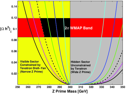
Figure 3: An analysis of the relic density of milli-charged particles arising in the StSM $Z^{\prime}$ model from the hidden sector for the case $\delta=0$, $M_{\chi}=$ 150 GeV, $\epsilon=(.01-.06)$ with .01 for the innermost curve and moving outward in steps of .01. The (yellow, grey) regions ($M_{Z^{\prime}}<2M_{\chi}$, $M_{Z^{\prime}}>2M_{\chi}$) correspond to a (narrow, broad) $Z^{\prime}$ resonance, and the WMAP-3 relic density constraints are satisfied for both a broad $Z^{\prime}$ resonance and a narrow $Z^{\prime}$ resonance as exhibited by the 2$\sigma$ WMAP-3 red and black bands. The region of narrow $Z^{\prime}$ resonance is constrained by the LEP and Tevatron data. The region in the $2\sigma$ WMAP-3 band can be probed via a dilepton signal as shown in Fig.(4). The red band to the left is excluded by the CDF 95% C.L. CDF data while the black band is consistent or on the edge thereof, with all constraints which can produce an observable dilepton signal.

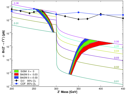
Figure 4: An exhibition of the dilepton signal $\sigma\cdot Br(Z^{\prime}\rightarrow l^{+}l^{-})$ at the Tevatron consistent with the WMAP-3 relic density constraint as a function of $M_{Z^{\prime}}$ when $2M_{\chi}=300$ GeV. The curves in ascending order are for values of $\bar{\epsilon}$ in the range $(0.01-0.06)$ in steps of 0.01. The dilepton signal has a dramatic fall as $M_{Z^{\prime}}$ crosses the point $2M_{\chi}=300$ GeV where the $Z^{\prime}$ decay into the hidden sector fermions is kinematically allowed, widening enormously the $Z^{\prime}$ decay width. The green shaded regions are where the WMAP-3 relic density constraints are satisfied for the case when there is no kinetic mixing. Red and blue regions are for the case when kinetic mixing is included. The DØ data set Abazov:2005pi was collected in the search for narrow resonances (RS) and is a stronger constraint to apply on this model than the recent CDF CDF data which put constraints on the parameter space when the $Z^{\prime}$ can decay only into matter in the visible sector.

The recent work of Ref. kctc has carried out an explicit analysis of putting a pair of Dirac fermions in the hidden sector, and made the interesting observation that for values $g_{X}Q_{X}\leq O(1)$ the decay width of $Z^{\prime}$ into the hidden sector Dirac fermions ($\chi$) can be of GeV size, and consequently the hidden matter can annihilate in sufficient amounts to satisfy the relic density. We have carried out a similar analysis using the thermal averaging procedure in the computation of the relic density as described in Appendix C. Our conclusions are in agreement with the analysis of Ref. kctc in the region of the parameter space investigated in Ref. kctc when no kinetic mixing is assumed in the absence of thermal averaging. In our work we take the kinetic mixing into account in the analysis of the relic density. We also make a further observation that there exists a significant region of the parameter space where it is possible to satisfy the relic density constraints and still have a narrow $Z^{\prime}$ resonance which can be detected at the Tevatron and at the LHC using the dilepton signal via a Drell-Yan process.

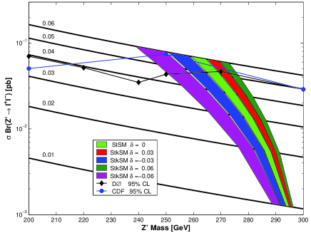
Figure 5: Same as Fig.(4) except that only the mass region with a detectable dilepton signal at the Tevatron is exhibited but additional $\delta$ values are included in the analysis. The plots show that the region allowed by WMAP-3 constraints moves to the right for positive $\delta$ and to the left for negative $\delta$. This phenomenon is explained in Appendix D. The inclusion of kinetic mixing is seen to enlarge the parameter space where the relic density constraints are satisfied and where an observable dilepton signal at the Tevatron can occur.

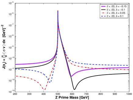
Figure 6: Illustration of the variation with $\delta$ of the thermally averaged cross section for the annihilation of milli-charged particles when $M_{\chi}=250$ GeV and $\bar{\epsilon}=.03$. The generic effect of $\delta$ is to modify the shape of $J(x_{f})$ and the region where the relic density constraints can be satisfied is enlarged. Further details are given in appendix D.

We give now further details of our relic density analysis. In the numerical analysis we will use $g_{X}=g^{SM}_{Y}$ and $Q_{X}=1$ unless stated otherwise. We begin by considering the case when $\delta=0$ which is the StSM case. Fig.(3) gives an analysis of the relic density as a function of $M_{Z^{\prime}}$ for the case $M_{\chi}=150$ GeV, and $\epsilon$ in the range $(0.01-0.06)$. Here one finds that the relic density is satisfied on two branches, one for $M_{Z^{\prime}}>2M_{\chi}$, and the other for $M_{Z^{\prime}}<2M_{\chi}$. In the region $M_{Z^{\prime}}>2M_{\chi}$ the relic density is satisfied over a broad range of $Z^{\prime}$ masses for appropriate $\epsilon$ values. In this region the decay width of the $Z^{\prime}$ is large, and thus the branching ratio into the visible sector is suppressed, which would make the dilepton signal from the $Z^{\prime}$ decay difficult to observe. This is exhibited in Fig.(4) where one finds that the dilepton signal essentially disappears in the region $M_{Z^{\prime}}>2M_{\chi}$. Next we examine the region $M_{Z^{\prime}}<2M_{\chi}$. Here one finds once again a satisfaction of the relic density even though the $Z^{\prime}$ mass lies below $2M_{\chi}$. The very sizable range of the $Z^{\prime}$ mass over which the relic density can be satisfied arises due to thermal averaging over the $Z^{\prime}$ pole. As expected in this region the $Z^{\prime}$ will appear as a sharp narrow resonance since the decay of the $Z^{\prime}$ into the hidden sector fermions is kinematically disallowed. An analysis of the dilepton signal for this case is also given in Fig.(4), and a more detailed view is given in Fig.(5), which shows that the Drell-Yan signal $p\bar{p}\to Z^{\prime}\to e^{+}e^{-}$ is enormously enhanced for $M_{Z^{\prime}}<2M_{\chi}$. Thus we have a region here of the parameter space where one will have a sharp resonance giving a visible dilepton signal while at the same time producing milli-charge dark matter consistent with WMAP-3.

We carry out a similar analysis for the case when the kinetic mixing parameter $\delta$ is non-vanishing. Fig.(6) gives an analysis of the effect of $\delta$ on the thermally averaged cross section $J(x_{f})$, defined in Appendix C, as a function of the $Z^{\prime}$ mass. One finds that $J(x_{f})$ is affected in a significant way by the change in $\delta$ and the particulars of the modification due to $\delta$ are explained in Appendix D. In Fig.(7) an analysis of relic density as a function of $M_{Z^{\prime}}$ is given for $\bar{\epsilon}=0.04$ and $\delta$ in the range $\delta=(.05-.25)$. The analysis shows the relic density exhibits a strong $\delta$ dependence. Quite significantly, the region in $M_{Z^{\prime}}$ over which the relic density can fall in the WMAP-3 region is widened. Once again, in the region $M_{Z^{\prime}}>2M_{\chi}$ the dilepton signal will be too dilute to be observable as shown in Fig.(7). On the other hand, in the region $M_{Z^{\prime}}<2M_{\chi}$, the $Z^{\prime}$ is a sharp narrow resonance since the $Z^{\prime}$ decay into the hidden sector fermions is kinematically disallowed. Thus the dilepton signal here is strong as can be seen in Fig.(4) and Fig.(5) and should be observable with sufficient luminosity.

An analysis for the case of the LHC in the Drell-Yan process $pp\to Z^{\prime}\to e^{+}e^{-}$, is given in Fig.(8). Here it is shown that the dilepton signal in the region $M_{Z^{\prime}}<2M_{\chi}$ consistent with the WMAP-3 constraints would be discernible with $10fb^{-1}$ of integrated luminosity for $\bar{\epsilon}\gtrsim.04$. The dilepton signal has a dramatic fall as $M_{Z^{\prime}}$ crosses the point $M_{Z^{\prime}}=2M_{\chi}$ beyond which the $Z^{\prime}$ decay into the hidden sector fermions is kinematically allowed, widening enormously the $Z^{\prime}$ decay width. The green shaded regions are where the WMAP-3 relic density constraints are satisfied for the case when there is no kinetic mixing. Red and blue regions are for the case when kinetic mixing is included. When computing the dilepton signal, a 20 GeV mass bin is used, and a 50% detector cut is assumed. The thick solid line corresponds to the LHC discovery limit with $10fb^{-1}$ of integrated luminosity expected in the first year run, and the criteria used for the discovery limit is $5\sqrt{N_{SM}}$ or 10 events, whichever is larger, where $N_{SM}$ is the number of SM background events. The analysis shows that data in the first year running at the LHC should be able to constrain the parameter space down to $\bar{\epsilon}\sim 0.04$ for $M_{\chi}=500$ GeV when $M_{Z^{\prime}}<1$ TeV.

An interesting issue concerns the question regarding how small $\bar{\epsilon}$ can be for WMAP-3 relic density constraints to be satisfied. Fig.(9) addresses this question where an analysis of the relic density is given when $\bar{\epsilon}=10^{-4}$. One finds satisfaction of the relic density in this case, and even smaller $\bar{\epsilon}$ were found admissible. Further, while the dilepton signal at the Tevatron in this case will be suppressed, it could still be visible at the LHC with sufficient luminosity.

Finally, we note that within the context of the Stueckelberg model it is possible to place indirect limits on the milli-charge coupling of hidden sector fermion with the photon from the Tevatron data. An analysis of the limits on the Stueckelberg mixing parameter $\epsilon$ was presented in fln1 for the case $\delta=0$. For this case, the milli-charge $Q_{milli}$, where $Q_{milli}e$ is the coupling of the photon with the hidden sector fermions (see Appendix D) is determined to be: $Q_{milli}\approx\epsilon$. Thus one may directly translate the limits obtained in fln1 to limits on the milli-charged coupling of the hidden fermion with the photon. In the context of the present analysis, the cross-section predictions given here, (as for example, in Fig.(5)) with their overlapping WMAP-3 bands, shows this explicitly.

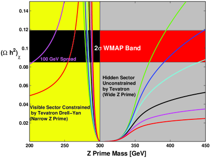
Figure 7: An analysis of the relic density of milli-charged particles for the case when kinetic mixing is included in the Stueckelberg $Z^{\prime}$ model. The analysis is done for $M_{\chi}=$ 150 GeV, $\bar{\epsilon}=.04$, and $\delta=(.05,.075,.10,.15,.20,.25)$, where the values are in descending order for $M_{Z^{\prime}}>300$ GeV. The red and black bands are the WMAP-3 constraints where the black band also produces an observable dilepton signal. The analysis shows that for $\bar{\epsilon}$ fixed, increasing $\delta$ increases the parameter space where the WMAP-3 relic density constraint is satisfied, while allowing for a detectable $Z$ prime signal as shown in Figs.(4,5).

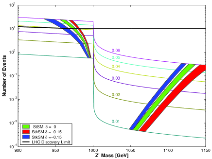
Figure 8: An exhibition of the dilepton signal as given by the number of events for 10$fb^{-1}$ of integrated luminosity at the LHC consistent with the WMAP-3 relic density constraint as a function of $M_{Z^{\prime}}$ when $M_{\chi}=500$ GeV. The curves in ascending order are for values of $\bar{\epsilon}$ in the range $(0.01-0.06)$ in steps of 0.01. Criteria set for the discovery limit are discussed in the text.

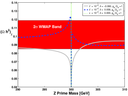
Figure 9: An analysis of the relic density of milli-charged particles for the case of a very small $\bar{\epsilon}$. One finds that even for this case one can satisfy the WMAP-3 relic density constraints. In this case the hidden sector fermion mass is predicted to be essentially $M_{Z^{\prime}}/2$. While the dilepton signal from the Drell-Yan process is too weak to be observable at the Tevatron, it is strong enough to be detectable at the LHC with sufficient integrated luminosity fln2 .

V Conclusion

In the above we have given an analysis of the Stueckelberg extension of the Standard Model with inclusion of the kinetic energy mixing in the $U(1)_{X}\times U(1)_{Y}$ sectors. Such kinetic mixings are quite generic in models with more than one $U(1)$ gauge group. It is shown that in the model with both the mass and kinetic mixing and in the absence of matter in the hidden sector, the sensitive parameter which measures the deviation from the Standard Model is given by $\bar{\epsilon}$ as defined by Eq. (21) which is a specific combination of $\epsilon$ and $\delta$, where $\epsilon$ measures the mass mixing and $\delta$ measures the kinetic mixing. However, when matter in the hidden sector is taken into account, electroweak physics depends on both $\epsilon$ and $\delta$. An analysis of the relic density of milli-charged dark matter which is generic in Stueckelberg extensions is given. Here our analysis is in agreement with the work of Ref. kctc for the case when no kinetic mixing is taken into account. Inclusion of the kinetic mixing is seen to increase the region of the parameter space where the relic density constraints consistent with WMAP-3 can be satisfied. We also analyze the $Z^{\prime}$ signal. As noted in Ref. kctc on the branch $M_{Z^{\prime}}>2M_{\chi}$ the dilepton signal from the $Z^{\prime}$ decay is too small to be observed at colliders, and our results are in agreement with this analysis. However, we note that on the branch $M_{Z^{\prime}}<2M_{\chi}$, there is a significant region of the parameter space where the relic density constraints can be satisfied and the dilepton signal from the $Z^{\prime}$ decay via the Drell-Yan process is strong enough to be observed at the Tevatron and at the LHC. The analysis also shows that relic density constraints can be satisfied for values of $\bar{\epsilon}$ as low as $10^{-4}$ and even smaller values are possible. An interesting issue concerns the detectability of such dark matter in laboratory experiments which might put further limits on the parameter space or on the component of the relic density such matter can constitute. However, such an investigation is outside the scope of this work.

Acknowledgments

This work was supported in part by the U.S. National Science Foundation under the grant NSF-PHY-0546568.

Appendix A: Details of the Stueckelberg extension with kinetic mixing

In this Appendix we give further details of the Stueckelberg extension with kinetic mixing. The mass matrix in the vector boson sector, after applying the transformation that diagonalizes the kinetic energy, is given by

$$M^{2}=K^{T}M_{St}^{2}K,$$ (13)

and we display its explicit form below

$$M^{2}=\left(\begin{array}[]{ccc}M_{1}^{2}\frac{(1-\epsilon\delta)^{2}}{1-\delta^{2}}+\frac{1}{4}\gamma^{2}v^{2}\frac{\delta^{2}(1-2\epsilon\delta+\epsilon^{2})}{1-\delta^{2}}&M_{1}^{2}\frac{\epsilon(1-\epsilon\delta)}{\sqrt{1-\delta^{2}}}-\frac{1}{4}\gamma^{2}v^{2}\frac{\delta(1-2\epsilon\delta+\epsilon^{2})}{\sqrt{1-\delta^{2}}}&\frac{1}{4}g_{2}\gamma v^{2}\frac{\delta\sqrt{1-2\epsilon\delta+\epsilon^{2}}}{\sqrt{1-\delta^{2}}}\\ M_{1}^{2}\frac{\epsilon(1-\epsilon\delta)}{\sqrt{1-\delta^{2}}}-\frac{1}{4}\gamma^{2}v^{2}\frac{\delta(1-2\epsilon\delta+\epsilon^{2})}{\sqrt{1-\delta^{2}}}&M_{1}^{2}\epsilon^{2}+\frac{1}{4}\gamma^{2}v^{2}(1-2\epsilon\delta+\epsilon^{2})&-\frac{1}{4}g_{2}\gamma v^{2}\sqrt{1-2\epsilon\delta+\epsilon^{2}}\\ \frac{1}{4}g_{2}\gamma v^{2}\frac{\delta\sqrt{1-2\epsilon\delta+\epsilon^{2}}}{\sqrt{1-\delta^{2}}}&-\frac{1}{4}g_{2}\gamma v^{2}\sqrt{1-2\epsilon\delta+\epsilon^{2}}&\frac{1}{4}g_{2}^{2}v^{2}\end{array}\right).$$ (14)

The eigenvalues of Eq. (14) are

$$M_{\gamma}^{2}=0,\hskip 7.11317ptM_{Z}^{2}=(q-p)/2,\hskip 7.11317ptM_{Z^{\prime}}^{2}=(q+p)/2,$$ (15)

where

$$p = \sqrt{\left(M_{1}^{2}\beta+\frac{\gamma^{2}\beta+g_{2}^{2}}{4}v^{2}\right)^{2}-4M_{1}^{2}\frac{\gamma^{2}+g_{2}^{2}}{4}v^{2}\beta},$$

$$q = M_{1}^{2}\beta+\frac{\gamma^{2}\beta+g_{2}^{2}}{4}v^{2}$$ (16)

and where $\beta=(1-2\epsilon\delta+\epsilon^{2})/(1-\delta^{2})$. As expected in the limit $\epsilon=0=\delta$ the Stueckelberg sector decouples from the SM sector and one gets

$$M_{Z}=\frac{\sqrt{g_{2}^{2}+\gamma^{2}}}{2}v,~{}~{}M_{Z^{\prime}}=M_{1}.$$ (17)

The expression for $M_{Z}$ of Eq. (17) is exactly the result in the SM. However, quite remarkably decoupling takes place also in the limit when $\epsilon$ and $\delta$ are non-vanishing but satisfy the relation $\epsilon=\delta$. Here, while the $\epsilon,\delta$ dependence persists in the $M^{2}$ mass matrix of Eq. (14), the eigenvalues are still given by Eq. (17) in this limit. Further, the coupling of the $Z$ boson to quarks and leptons reduces to that of the SM in this limit. One may understand this result by examining the explicit form of the transformation matrix of Eq. (II) which for the case $\epsilon=\delta$ becomes

$$T=\left(\begin{array}[]{ccc}1&\frac{\gamma}{\sqrt{g_{2}^{2}+\gamma^{2}}}\frac{\delta}{\sqrt{1-\delta^{2}}}&-\frac{g_{2}}{\sqrt{g_{2}^{2}+\gamma^{2}}}\frac{\delta}{\sqrt{1-\delta^{2}}}\\ 0&-\frac{\gamma}{\sqrt{g_{2}^{2}+\gamma^{2}}}\frac{1}{\sqrt{1-\delta^{2}}}&\frac{g_{2}}{\sqrt{g_{2}^{2}+\gamma^{2}}}\frac{1}{\sqrt{1-\delta^{2}}}\\ 0&\frac{g_{2}}{\sqrt{g_{2}^{2}+\gamma^{2}}}&\frac{\gamma}{\sqrt{g_{2}^{2}+\gamma^{2}}}\end{array}\right).$$ (18)

A direct substitution in the $Z$ and $Z^{\prime}$ couplings then shows that they are identical to the case of the SM. These analytic forms explain the limits seen numerically in the analysis of Fig.(1).

Next we consider the case with arbitrary mass mixing and kinetic mixing. Here before diagonalizing the mass matrix it is convenient to perform the following orthogonal transformation $(O)$ given by

$$O=\left(\begin{array}[]{ccc}\sqrt{1-\delta^{2}}&-\delta&0\\ \delta&\sqrt{1-\delta^{2}}&0\\ 0&0&1\end{array}\right),$$ (19)

which transforms the mass matrix to $\mathcal{M}^{2}=O^{T}M^{2}O$

$$\mathcal{M}^{2}=\left(\begin{array}[]{ccc}M_{1}^{2}&M_{1}^{2}\bar{\epsilon}&0\\ M_{1}^{2}\bar{\epsilon}&M_{1}^{2}\bar{\epsilon}^{2}+\frac{v^{2}}{4}\gamma^{2}(1+\bar{\epsilon}^{2})&-\frac{v^{2}}{4}g_{2}\gamma\sqrt{1+\bar{\epsilon}^{2}}\\ 0&-\frac{v^{2}}{4}g_{2}\gamma\sqrt{1+\bar{\epsilon}^{2}}&\frac{v^{2}}{4}g_{2}^{2}\end{array}\right)$$ (20)

where $\bar{\epsilon}$ is defined so that

$$\bar{\epsilon}=\frac{\epsilon-\delta}{\sqrt{1-\delta^{2}}}.$$ (21)

We note that the mass matrix Eq. (20) looks exactly the same as for the mass matrix one has if there was just the Stueckelberg mass mixing except that $\epsilon$ is replaced by $\bar{\epsilon}$. Thus the orthogonal matrix which diagonalizes Eq. (20) will be the same as for the StSM case except that the free parameter is changed from $\epsilon$ to $\bar{\epsilon}$. We parameterize the rotation matrix $\cal R$ defined by ${\cal R}^{T}{\cal M}^{2}{\cal{R}}=Diag(M_{Z^{\prime}}^{2},M_{Z}^{2},0)$ by the following

$${\cal R}=\left[\matrix{\cos\psi\cos\phi-\sin\theta\sin\phi\sin\psi&\sin\psi\cos\phi+\sin\theta\sin\phi\cos\psi&-\cos\theta\sin\phi\cr\cos\psi\sin\phi+\sin\theta\cos\phi\sin\psi&\sin\psi\sin\phi-\sin\theta\cos\phi\cos\psi&\cos\theta\cos\phi\cr-\cos\theta\sin\psi&\cos\theta\cos\psi&\sin\theta}\right],$$

where the angles are defined so that

$$\tan\theta = \frac{\gamma}{g_{2}},~{}~{}~{}~{}\tan\phi=\bar{\epsilon},~{}~{}~{}~{}\tan 2\psi=\frac{2\sin\theta M_{0}^{2}\bar{\epsilon}}{M_{1}^{2}-M_{0}^{2}+(M_{1}^{2}+M_{0}^{2}-M_{W}^{2})\bar{\epsilon}^{2}},$$ (22)

and $M_{0}=M_{Z}(\epsilon=\delta)=v\sqrt{g_{2}^{2}+\gamma^{2}}/2$, $M_{W}=g_{2}v/2$. The transformation relating the initial basis and the final diagonal basis is $V=[K(\delta)O(\delta){\cal{R}}(\bar{\epsilon})]E$, where $V^{T}=(C,B,A^{3})$, and $E^{T}=(Z^{\prime},Z,A_{\gamma})$. The neutral current interaction can now be written in the form

$$\mathcal{L}_{NC}=J^{T}S(\bar{\epsilon},\delta){\cal{R}}(\bar{\epsilon})E$$ (23)

where $J^{T}=(g_{X}J_{X},\gamma J_{Y},g_{2}J_{2}^{3})$, and $S$ is given by

$$S(\bar{\epsilon},\delta)=\left[\matrix{1&-{\delta}/{\sqrt{1-\delta^{2}}}&0\cr 0&\sqrt{1+\bar{\epsilon}^{2}}&0\cr 0&0&1\cr}\right].$$ (24)

When $J_{X}=0$, one finds that the neutral current interaction of Eq. (23) has no dependence on $\delta$. Expressing the tree level interaction in terms of the reduced vector and axial vector couplings as defined in Eq. (10), we find

$$v_{f} = \cos\psi\left[\left(1-\bar{\epsilon}\sin\theta\tan\psi\right)T_{f}^{3}-2\sin^{2}\theta\left(1-\bar{\epsilon}\csc\theta\tan\psi\right)Q_{f}\right],$$ (25)

$$a_{f} = \cos\psi\left[1-\bar{\epsilon}\sin\theta\tan\psi\right]T_{f}^{3},$$ (26)

$$v^{\prime}_{f} = -\cos\psi\left[\left(\tan\psi+\bar{\epsilon}\sin\theta\right)T_{f}^{3}-2\sin^{2}\theta\left(\bar{\epsilon}\csc\theta+\tan\psi\right)Q_{f}\right],$$ (27)

$$a^{\prime}_{f} = -\cos\psi\left[\tan\psi+\bar{\epsilon}\sin\theta\right]T_{f}^{3}.$$ (28)

Thus in the absence of the hidden sector matter, the effect on the neutral current sector of including the kinetic mixing in the Stueckelberg model, is the replacement of $\epsilon$ by $\bar{\epsilon}$, and in the limit $\bar{\epsilon}\to 0$ the $Z$ couplings of the SM are recovered. However, with the inclusion of matter in the hidden, i.e., $J_{X}\neq 0$, the neutral current sector will depend on both $\bar{\epsilon}$ and $\delta$. We exhibit this below

$${\cal{L}}_{NC}={\cal{L}}_{NC}(J_{X}=0)+g_{X}J_{X}^{\mu}\biggr{[}\left({\cal{R}}_{11}-S_{\delta}{\cal{R}}_{21}\right)Z^{\prime}_{\mu}+\left({\cal{R}}_{12}-S_{\delta}{\cal{R}}_{22}\right)Z_{\mu}+\left({\cal{R}}_{13}-S_{\delta}{\cal{R}}_{23}\right)A^{\gamma}_{\mu}\biggr{]}$$ (29)

where $S_{\delta}$ appears in Eq.(29), and is as defined in Sec.(II). In this case the decay modes of $Z^{\prime}$ depend on both $\epsilon$ and $\delta$ and an analysis of the branching ratios should reveal the presence of kinetic mixing.

Further, as discussed in Sec.(IV) and in Appendix D, the relic density analysis depends sensitively on $\delta$.

Appendix B: On the origin of
milli-charged matter

In this Appendix we illustrate the mechanism which generates the milli-charge in the context of the analysis of this paper. We start with the kinetic mixing model holdom with two gauge fields $A_{1\mu},A_{2\mu}$ corresponding to the gauge groups $U(1)$ and $U(1)^{\prime}$. We choose the following Lagrangian $\mathcal{L}=\mathcal{L}_{0}+\mathcal{L}_{1}$ where

$$\mathcal{L}_{0} = -\frac{1}{4}F_{1\mu\nu}F_{1}^{\mu\nu}-\frac{1}{4}F_{2\mu\nu}F_{2}^{\mu\nu}-\frac{\delta}{2}F_{1\mu\nu}F_{2}^{\mu\nu},$$

$$\mathcal{L}_{1} = J^{\prime}_{\mu}A_{1}^{\mu}+J_{\mu}A_{2}^{\mu}.$$ (30)

To put the kinetic energy term in its canonical form, one may use the transformation

$$\left[\matrix{A_{1}^{\mu}\cr A_{2}^{\mu}}\right]\to K_{0}\left[\matrix{A^{\prime\mu}\cr A^{\mu}}\right],~{}~{}K_{0}=\left[\matrix{\frac{1}{\sqrt{1-\delta^{2}}}&0\cr\frac{-\delta}{\sqrt{1-\delta^{2}}}&1}\right].$$ (31)

However, the transformation that canonically diagonalizes the kinetic energy is not unique. Thus, for example, $K=K_{0}R$ instead of $K_{0}$ would do as well where $R$ is an orthogonal matrix

$$R=\left[\matrix{\cos\theta&-\sin\theta\cr\sin\theta&\cos\theta}\right].$$ (32)

Here $\mathcal{L}_{1}$ is given by

$$\mathcal{L}_{1}=A^{\prime\mu}\left[\frac{\cos\theta}{\sqrt{1-\delta^{2}}}J^{\prime}_{\mu}+\left(\sin\theta-\frac{\cos\theta\delta}{\sqrt{1-\delta^{2}}}\right)J_{\mu}\right]$$

$$+A^{\mu}\left[-\frac{\sin\theta}{\sqrt{1-\delta^{2}}}J^{\prime}_{\mu}+\left(\cos\theta+\frac{\sin\theta\delta}{\sqrt{1-\delta^{2}}}\right)J_{\mu}\right].$$ (33)

In this case we see that each of the massless states interacts with the sources $J$ and $J^{\prime}$. However, one may choose $\theta$ to get asymmetric solutions. For instance for the case $\theta=\arctan\left[\delta/\sqrt{1-\delta^{2}}\right]$ one has

$$\mathcal{L}_{1}=A^{\mu}\left[\frac{1}{\sqrt{1-\delta^{2}}}J_{\mu}-\frac{\delta}{\sqrt{1-\delta^{2}}}J^{\prime}_{\mu}\right]+A^{\prime\mu}J^{\prime}_{\mu}.$$ (34)

In this case while $A^{\prime}$ interacts only with the source $J^{\prime}$, $A$ interacts with both $J$ and $J^{\prime}$, with the coupling to the source $J^{\prime}$ proportional to the kinetic mixing parameter $\delta$. We identify $A$ with the physical photon field, $J$ with the physical source arising from quarks and leptons, while $A^{\prime}$ is the orthogonal massless state, and $J^{\prime}$ is the source in the hidden sector. Here the coupling of the photon with the hidden sector is proportional to $\delta$ and thus the hidden sector is milli-charged if $\delta$ is small.

Next we consider a model with kinetic mixing where a Stueckelberg mechanism generates a mass term of the type considered in Eq. (1)

$${\cal{L}}_{\rm{Mass}}=-\frac{1}{2}M_{1}^{2}A_{1\mu}A_{1}^{\mu}-\frac{1}{2}M_{2}^{2}A_{2\mu}A_{2}^{\mu}-M_{1}M_{2}A_{1\mu}A_{2}^{\mu}.\\$$

In this case diagonalizaton of the mass matrix fixes $\theta$ so that

$$\theta=\arctan\left[\frac{\epsilon\sqrt{1-\delta^{2}}}{1-\delta\epsilon}\right],$$ (35)

and the interaction Lagrangian is given by

$${\cal{L}}_{1} = \frac{1}{\sqrt{1-2\delta\epsilon+\epsilon^{2}}}\left(\frac{\epsilon-\delta}{\sqrt{1-\delta^{2}}}J_{\mu}+\frac{1-\delta\epsilon}{\sqrt{1-\delta^{2}}}J_{\mu}^{\prime}\right)A_{M}^{\mu}$$ (36)

$$+ \frac{1}{\sqrt{1-2\delta\epsilon+\epsilon^{2}}}\left(J_{\mu}-\epsilon J_{\mu}^{\prime}\right)A^{\mu}_{\gamma}.$$

Here for the case $\epsilon=0$ one finds that the massless state, the photon $A_{\gamma}^{\mu}$, no longer couples with the hidden sector, while the massive mode $A_{M}^{\mu}$ couples with both the visible sector via $J$ and with the hidden sector via $J^{\prime}$. We conclude, therefore, that in the absence of the Stueckelberg mass mixing, for the case when only one mode is massless, there are no milli-charged particles coupled to the photon field. Thus milli-charge couplings appear in this case only when the Stueckelberg mixing parameter $\epsilon$ is introduced. Thus for the case when only one mode is massless the kinetic mixing by itself does not allow milli-charges but the Stueckelberg mass mixing model does.

Appendix C: Analysis of relic density of milli-charged dark matter in the hidden sector

The analysis of relic density involves the integral of the thermally averaged cross section from the current temperature to the freeze out such that Nath:1992ty

$$J(x_{f})=\int_{0}^{x_{f}}\langle\sigma v\rangle dx.$$ (37)

Here $\sigma$ is the annihilation cross section for the process $\chi\bar{\chi}\to f\bar{f}$ where $f$ denotes a quark or a lepton, and $v$ is the relative velocity of the annihilating Dirac fermions $\chi$ and $\bar{\chi}$. We use the notation, $x=T/M_{\chi}$ in units where the Boltzman constant is unity, and $x_{f}$ is the value of $x$ at the freeze out temperature. The thermally averaged cross section $\langle\sigma v\rangle$ is given by

$$\langle\sigma v\rangle=\frac{\int_{0}^{\infty}dvv^{2}(\sigma v)e^{-(v^{2}/4x)}}{\int_{0}^{\infty}dvv^{2}e^{-(v^{2}/4x)}}.$$ (38)

Using the analysis of Ref. kctc $(\sigma v)$ is given by

$$(\sigma v)\simeq f_{1}(s)({\xi}^{2}_{L}+{\xi}^{2}_{R})+f_{2}(s)({\xi}_{L}{\xi}_{R})$$ (39)

where the functions $f_{1}$ and $f_{2}$ depend on the square of the CM energy $s$ and are given by

$$f_{1}(s) = C_{f}v\frac{\beta_{f}}{s\beta_{\chi}}[s^{2}(1+\frac{1}{3}\beta^{2}_{f}\beta^{2}_{\chi})+4M^{2}_{\chi}(s-2m^{2}_{f})]$$

$$f_{2}(s) = C_{f}v\frac{\beta_{f}}{s\beta_{\chi}}[8m^{2}_{f}(s+2M^{2}_{\chi})].$$ (40)

Here $C_{f}=N_{f}/(32\pi)$, $N_{f}=(1,3)$ for $f=(\rm lepton,\rm quark)$, $\xi_{L}$ and $\xi_{R}$ are as defined in Ref. kctc and contain the photon, the $Z$ and the $Z^{\prime}$ poles, the latter augmented with a Breit-Wigner distribution for thermal averaging, as the largest contribution to $\langle\sigma v\rangle$ for $4M^{2}_{\chi}\gg M^{2}_{Z}$ arises from integration over the $Z^{\prime}$ pole. In the vicinity of the $Z^{\prime}$ pole we can expand $(\sigma v)$ as follows

$$(\sigma v)\simeq C_{1}+C_{2}v^{2}+\frac{C_{3}M^{-4}_{\chi}+C_{4}M^{-2}_{\chi}v^{2}}{(v^{2}-\epsilon_{R})^{2}+\gamma^{2}_{R}}$$ (41)

where $\epsilon_{R}$ and $\gamma_{R}$ are given by

$$\epsilon_{R}=(M_{Z^{\prime}}^{2}-4M_{\chi}^{2})/M_{\chi}^{2}~{},~{}~{}~{}\gamma_{R}=\Gamma_{Z^{\prime}}M_{Z^{\prime}}/M_{\chi}^{2}$$ (42)

and where $C_{i}(i=1-4)$ can be read off from the expansion of $s$ in Eq. (39) and Eq. (40). Using the technique of Ref. Nath:1992ty the integral $J(x_{f})$ is given by

$$J(x_{f})=x_{f}C_{1}+3x^{2}_{f}C_{2}+\frac{1}{2\sqrt{\pi}M^{4}_{\chi}}\biggr{[}\frac{C_{3}}{{\epsilon}_{R}}I_{2}+M^{2}_{\chi}C_{4}(I_{1}+I_{2})\biggr{]}$$ (43)

where

$$I_{1}=\frac{1}{2}\int_{0}^{\infty}dyy^{-1/2}e^{-y}Ln\biggr{[}\frac{(4x_{f}y-\epsilon_{R})^{2}+\gamma^{2}_{R}}{\epsilon^{2}_{R}+\gamma^{2}_{R}}\biggr{]},$$ (44)

$$I_{2}=\frac{\epsilon_{R}}{\gamma_{R}}\int_{0}^{\infty}dyy^{-1/2}e^{-y}\biggr{[}\arctan\biggr{[}\frac{4x_{f}y-\epsilon_{R}}{\gamma_{R}}\biggr{]}+\arctan\biggr{[}\frac{\epsilon_{R}}{\gamma_{R}}\biggr{]}\biggr{]}.$$ (45)

From the above one then obtains the relic density using the standard relations as discussed, for example, in Ref. Nath:1992ty .

Appendix D: The effect of $\delta$ on the cross section

The kinetic mixing parameter $\delta$ enters Eq. (29) via the hidden sector where

$$\mathcal{L}_{NC}^{\rm{hid}} = \bar{\chi}\gamma^{\mu}\left[\epsilon_{Z^{\prime}}^{\chi}Z^{\prime}_{\mu}+\epsilon_{Z}^{\chi}Z_{\mu}+\epsilon_{\gamma}^{\chi}A^{\gamma}_{\mu}\right]\chi.$$ (46)

In the limit $\bar{\epsilon},\delta\ll 1$, the couplings to leading order are

$$\epsilon_{Z^{\prime}}^{\chi} = g_{X}Q_{X}\left[{\cal{R}}_{11}-\frac{\delta}{\sqrt{1-\delta^{2}}}{\cal{R}}_{21}\right]\simeq g_{X}Q_{X},$$ (47)

$$\epsilon_{Z}^{\chi} = g_{X}Q_{X}\left[{\cal{R}}_{12}-\frac{\delta}{\sqrt{1-\delta^{2}}}{\cal{R}}_{22}\right]\simeq\bar{\epsilon}g_{X}Q_{X}\sin\theta\left[1+\frac{\delta}{\bar{\epsilon}}\right],$$ (48)

$$\epsilon_{\gamma}^{\chi} = g_{X}Q_{X}\left[{\cal{R}}_{13}-\frac{\delta}{\sqrt{1-\delta^{2}}}{\cal{R}}_{23}\right]\simeq-\bar{\epsilon}g_{X}Q_{X}\cos\theta\left[1+\frac{\delta}{\bar{\epsilon}}\right].$$ (49)

For the purpose of illustration in this Appendix, and only here, we will work in the limit $m_{f}\sim 0$ , $v\sim 0$ and $\Gamma_{Z^{\prime}}\sim 0$ so that

$$\sigma v\simeq\frac{M_{\chi}^{2}N_{f}}{2\pi}\biggr{[}\xi_{L}^{2}+\xi_{R}^{2}\biggr{]},$$ (50)

where for $4M_{\chi}^{2}\gg M_{Z}^{2}$,

$$\xi_{L,R} \simeq \frac{\epsilon_{\gamma}^{\chi}eQ_{\rm em}^{f}}{4M_{\chi}^{2}}+\frac{\epsilon_{Z}^{\chi}\epsilon^{f_{L,R}}_{Z}}{4M_{\chi}^{2}-M_{Z}^{2}}+\frac{\epsilon_{Z^{\prime}}^{\chi}\epsilon^{f_{L,R}}_{Z^{\prime}}}{4M_{\chi}^{2}-M_{Z^{\prime}}^{2}}$$ (51)

$$= \alpha_{L,R}+\frac{\beta_{L,R}}{4M_{\chi}^{2}-M_{Z^{\prime}}^{2}}.$$

Defining $x=(4M_{\chi}^{2}-M_{Z^{\prime}}^{2})$, $\sigma v$ can be further simplified as

$$\sigma v \simeq a+\frac{2b}{x}+\frac{c}{x^{2}},$$ (52)

where $a,b,c$ are functions of $\eta=(1+\delta/\bar{\epsilon})$ and are given by

$$a = \frac{M_{\chi}^{2}N_{f}}{2\pi}(\alpha_{L}^{2}+\alpha_{R}^{2})$$

$$b = \frac{M_{\chi}^{2}N_{f}}{2\pi}(\alpha_{L}\beta_{L}+\alpha_{R}\beta_{R}),$$

$$c = \frac{M_{\chi}^{2}N_{f}}{2\pi}(\beta_{L}^{2}+\beta_{R}^{2}).$$ (53)

The $\eta$ dependence can then be read off so that $a(\eta)=\eta^{2}a(1),b(\eta)=\eta b(1),c(\eta)=c(1)$. The cross section described by Eq. (52) has a dip when $x_{min}=-c/b$ which gives $(\sigma v)_{min}=a-b^{2}/c$. Now $x_{min}$ and $(\sigma v)_{min}$ have an $\eta$ dependence of the form $x_{min}(\eta)=x_{min}(1)/\eta$, and $(\sigma v)_{min}(\eta)=\eta^{2}(\sigma v)_{min}(1)$ which implies that for the case $\eta>1$ a larger $\eta$ shrinks $x_{min}$ and moves the dip closer to the resonance point. At the same time it also increases $(\sigma v)_{min}$. More interestingly, a negative $\eta$ will switch the dip to the other side of the resonance. These effects are illustrated in the analysis of Fig.(6). The analysis above explains why the inclusion of kinetic mixing enhances the region where the relic density constraint is satisfied.

References

- (1) B. Körs and P. Nath, Phys. Lett. B 586, 366 (2004) [hep-ph/0402047].
- (2) B. Körs and P. Nath, JHEP 0412 (2004) 005 [hep-ph/0406167].
- (3) B. Körs and P. Nath, JHEP 0507, 069 (2005) [hep-ph/0503208].
- (4) D. Feldman, Z. Liu and P. Nath, Phys. Rev. Lett. 97, 021801 (2006) [hep-ph/0603039].
- (5) D. Feldman, Z. Liu and P. Nath, JHEP 0611, 007 (2006) [arXiv:hep-ph/0606294].
- (6) T. Appelquist, H. C. Cheng and B. A. Dobrescu, Phys. Rev. D 64, 035002 (2001); M. Battaglia, A. Datta, A. De Roeck, K. Kong and K. T. Matchev, JHEP 0507, 033 (2005) [arXiv:hep-ph/0502041]; G. Burdman, B. A. Dobrescu and E. Ponton, Phys. Rev. D 74, 075008 (2006)
- (7) B. Holdom, B. Holdom, Phys. Lett. B 166, 196 (1986); Phys. Lett. B 259, 329 (1991).
- (8) J. Kumar and J. D. Wells, Phys. Rev. D 74, 115017 (2006) [arXiv:hep-ph/0606183].
- (9) W. F. Chang, J. N. Ng and J. M. S. Wu, Phys. Rev. D 74 (2006) 095005 [arXiv:hep-ph/0608068].
- (10) A. Ferroglia, A. Lorca and J. J. van der Bij, arXiv:hep-ph/0611174.
- (11) L. Randall and R. Sundrum, Phys. Rev. Lett. 83, 3370 (1999).
- (12) H. Davoudiasl, J. L. Hewett and T. G. Rizzo, Phys. Rev. Lett. 84, 2080 (2000).
- (13) D. M. Ghilencea, L. E. Ibanez, N. Irges and F. Quevedo, JHEP 0208 (2002) 016; D. M. Ghilencea, Nucl. Phys. B 648 (2003) 215.
- (14) L. E. Ibanez, F. Marchesano and R. Rabadan, JHEP 0111 (2001) 002; R. Blumenhagen, V. Braun, B. Körs and D. Lüst, hep-th/0210083; I. Antoniadis, E. Kiritsis, J. Rizos and T. N. Tomaras, Nucl. Phys. B 660, 81 (2003); C. Coriano, N. Irges and E. Kiritsis, arXiv:hep-ph/0510332; R. Blumenhagen, B. Kors, D. Lust and S. Stieberger, arXiv:hep-th/0610327.
- (15) P. Anastasopoulos, M. Bianchi, E. Dudas and E. Kiritsis, JHEP 0611, 057 (2006) [hep-th/0605225]. P. Anastasopoulos, T. P. T. Dijkstra, E. Kiritsis and A. N. Schellekens, Nucl. Phys. B 759, 83 (2006) [hep-th/0605226].
- (16) C. Coriano and N. Irges, arXiv:hep-ph/0612128; C. Coriano and N. Irges, arXiv:hep-ph/0612140; C. Coriano, N. Irges and S. Morelli, arXiv:hep-ph/0701010;
- (17) P. Anastasopoulos, arXiv:hep-th/0701114.
- (18) D. Feldman, B. Kors and P. Nath, Phys. Rev. D 75, 023503 (2007) [arXiv:hep-ph/0610133].
- (19) D. N. Spergel et al., astro-ph/0603449.
- (20) K. Cheung and T. C. Yuan, JHEP 0703, 120 (2007) [arXiv:hep-ph/0701107].
- (21) K. S. Babu, C. F. Kolda and J. March-Russell, Phys. Rev. D 57, 6788 (1998), hep-ph/9710441; R. Foot and X. G. He, Phys. Lett. B 267, 509 (1991).
- (22) K.R. Dienes, C. Kolda, and J. March-Russell, Nucl. Phys 492, 104 (1997)
- (23) M. Cvetic and P. Langacker, Mod. Phys. Lett. A 11 (1996) 1247 [hep-ph/9602424]; A.E. Farragi and M. Masip, Phys. Lett. B 388 (1996) 524 [hep-ph/9604302].
- (24) V. Barger, C. Kao, P. Langacker and H. S. Lee, Phys. Lett. B 600, 104 (2004) [hep-ph/0408120];
- (25) A. Leike, Phys. Rept. 317, 143 (1999), hep-ph/9805494;
- (26) For early work on the Stueckelberg mechanism see, E.C.G. Stueckelberg, Helv. Phys. Acta. 11 (1938) 225; V. I. Ogievetskii and I.V. Polubarinov, JETP 14 (1962) 179; A. Chodos and F. Cooper, Phys. Rev. D 3, 2461 (1971); M. Kalb and P. Ramond, Phys. Rev. D 9, 2273 (1974); T. J. Allen, M. J. Bowick and A. Lahiri, Mod. Phys. Lett. A 6 (1991) 559.
- (27) P. Nath and M. Yamaguchi, Phys. Rev. D 60, 116004 (1999) [arXiv:hep-ph/9902323].
- (28) S. Eidelman et al. [Particle Data Group], Phys. Lett. B 592, 1 (2004).
- (29) [ALEPH Collaboration], hep-ex/0509008.
- (30) [LEP Collaboration], arXiv:hep-ex/0312023; [ALEPH Collaboration], arXiv:hep-ex/0609051.
- (31) H. Goldberg and L. J. Hall, Phys. Lett. B 174, 151 (1986).
- (32) E. Golowich and R. W. Robinett, Phys. Rev. D 35, 391 (1987).
- (33) R. N. Mohapatra and I. Z. Rothstein, Phys. Lett. B 247, 593 (1990).
- (34) S. Davidson and M. E. Peskin, Phys. Rev. D 49, 2114 (1994) [arXiv:hep-ph/9310288].
- (35) R. Foot, G. C. Joshi, H. Lew and R. R. Volkas, Mod. Phys. Lett. A 5, 95 (1990) [Erratum-ibid. A 5, 2085 (1990)].
- (36) D. O. Caldwell, R. M. Eisberg, D. M. Grumm, M. S. Witherell, B. Sadoulet, F. S. Goulding and A. R. Smith, Phys. Rev. Lett. 61, 510 (1988).
- (37) M. I. Dobroliubov and A. Y. Ignatiev, Phys. Rev. Lett. 65, 679 (1990).
- (38) R. Foot, arXiv:hep-ph/9407331.
- (39) S. Davidson, S. Hannestad and G. Raffelt, JHEP 0005, 003 (2000) [arXiv:hep-ph/0001179].
- (40) M. L. Perl, P. C. Kim, V. Halyo, E. R. Lee, I. T. Lee, D. Loomba and K. S. Lackner, Int. J. Mod. Phys. A 16, 2137 (2001) [arXiv:hep-ex/0102033].
- (41) A. A. Prinz et al., Phys. Rev. Lett. 81, 1175 (1998) [arXiv:hep-ex/9804008].
- (42) S. L. Dubovsky, D. S. Gorbunov and G. I. Rubtsov, JETP Lett. 79, 1 (2004) [Pisma Zh. Eksp. Teor. Fiz. 79, 3 (2004)] [arXiv:hep-ph/0311189].
- (43) E. Masso and J. Redondo, Phys. Rev. Lett. 97, 151802 (2006) [arXiv:hep-ph/0606163].
- (44) S. A. Abel and B. W. Schofield, Nucl. Phys. B 685, 150 (2004) [arXiv:hep-th/0311051].
- (45) S. A. Abel, J. Jaeckel, V. V. Khoze and A. Ringwald, arXiv:hep-ph/0608248.
- (46) M. Ahlers, H. Gies, J. Jaeckel and A. Ringwald, arXiv:hep-ph/0612098.
- (47) A. Badertscher et al., Phys. Rev. D 75, 032004 (2007); S. N. Gninenko, N. V. Krasnikov and A. Rubbia, Phys. Rev. D 75, 075014 (2007)
- (48) CDF Public Note : CDF/ANAL/EXOTIC/8421
- (49) V. M. Abazov et al. [D0 Collaboration], Phys. Rev. Lett. 95, 091801 (2005) [arXiv:hep-ex/0505018].
- (50) P. Nath and R. Arnowitt, Phys. Rev. Lett. 70 (1993) 3696 [arXiv:hep-ph/9302318].; See also, H. Baer and M. Brhlik, Phys. Rev. D 53 (1996) 597 [arXiv:hep-ph/9508321] ; V. D. Barger and C. Kao, Phys. Rev. D 57 (1998) 3131 [arXiv:hep-ph/9704403]. For early work see, K. Griest and D. Seckel, Phys. Rev. D 43 (1991) 3191; P. Gondolo and G. Gelmini, Nucl. Phys. B 360 (1991) 145.