Signatures of Spherical Compactification at the LHC

Abstract

TeV-scale extra dimensions may play an important role in electroweak or supersymmetry breaking. We examine the phenomenology of such dimensions, compactified on a sphere $S^{n}$, $n\geq 2$, and show that they possess distinct features and signatures. For example, unlike flat toroidal manifolds, spheres do not trivially allow fermion massless modes. Acceptable phenomenology then generically leads to “non-universal” extra dimensions with “pole-localized” 4-$d$ fermions; the bosonic fields can be in the bulk. Due to spherical symmetry, some Kaluza-Klein (KK) modes of bulk gauge fields are either stable or extremely long-lived, depending on the graviton KK spectrum. Using precision electroweak data, we constrain the lightest gauge field KK modes to lie above $\simeq 4$ TeV. We show that some of these KK resonances are within the reach of the LHC in several different production channels. The models we study can be uniquely identified by their collider signatures.

I Introduction

A great deal of attention has been devoted to the theoretical development of models with extra dimensions over the past several years. Motivated by a desire to explain the gauge hierarchy problem in the Standard Model (SM), various scenarios with one or more extra dimensions have been proposed. These models generally give rise to new phenomena not far above the weak scale. Nearly all cases that have been studied are endowed with extra dimensions that are: (1) large and toroidal, or (2) TeV-scale and toroidal, or (3) a slice of AdS₅.

Of the above categories, only (3) allows for a curved background. This geometry is the basis of the Randall-Sundrum (RS) model Randall:1999ee which requires a 5-$d$ spacetime with constant negative curvature. Given that spheres provide a simple, highly symmetric, and yet non-trivial (with positive constant curvature) departure from either the RS or toroidal geometries, it would be interesting to consider them as compactification manifolds. TeV-scale phenomenology of compactification on spheres has so far received very little attention; for some work in this direction see Refs. Lim ; Leblond:2001ex . Perhaps this is due to the relative simplicity of the analysis with a toroidal geometry, in conjunction with the expectation that spherical extra dimensions would offer no new qualitative features and only yield trivial numerical modulations.

In this work, we consider models with extra dimensions compactified on spheres $S^{n}$, $n\geq 2$, and show that the above expectation is rather naive, since a number of new features will be shown to arise. First of all, it has been demonstrated that if fermions propagate on $S^{n}$, the low energy 4-$d$ spectrum does not include a chiral zero mode Camporesi:1995fb ; Abrikosov:2001nj . For example, in the case of $S^{2}$, the lightest Kaluza-Klein (KK) mode of a 6-$d$ fermion with a zero bulk mass term has a mass $1/(2R)$, where $R$ is the radius of the sphere. Hence, we are naturally led to a scenario with “non-universal” extra dimensions in which the fermions remain 4-$d$ fields. The easiest way to accomplish this is to have fermions localized at some point on the surface of the $S^{n}$. A priori, all such points are identical by spherical symmetry and the arbitrary choice of co-ordinates. Once a particular point is chosen for fermion localization we can, for convenience of calculations, identify it with one of the poles of the sphere. This fermion localization can occur in a number of ways, i.e., through orbifolding and/or the existence of a 3-brane at a particular point in the higher dimensional space. The details of this particular mechanism are beyond the scope of the present analysis and will not concern us here.

In this paper, we will therefore examine the consequences of placing the gauge, and possibly Higgs, sectors of the SM on a sphere. Hence, we assume that $R^{-1}\gtrsim$ TeV, to avoid conflictLEPEWWG with low energy data. TeV-scale extra dimensions may play a role in electroweak symmetry or supersymmetry breaking Antoniadis:1990ew , and hence may be discovered in upcoming LHC experiments colliders . We focus on the simple case with $n=2$ where all the important features can be inferred from the properties of the familiar spherical harmonics. Our results can be easily extended to the case of $n>2$. Upon dimensional reduction, various KK towers appear in the 4-$d$ description. Due to the spherical symmetry of the underlying geometry, there are preserved quantum numbers that ensure the stability of some KK modes. As we will see, the $S^{2}$ spherical $SU(2)$ symmetry will be partially broken down to a $U(1)$ by the localization of the fermions at the pole(s).

Exactly which KK states remain stable is a question of kinematics as well. Here, quantum corrections to the simple KK spectrum can affect our conclusions. Also, we note that the stable gauge sector modes can become destabilized if the KK graviton spectrum allows “gravitational” decays of the gauge KK modes. The resulting lifetimes are found to be reasonably long and these particles are stable on collider time scales, but generally not cosmologically. These issues have also been noted in the previously studied toroidal compactifications Feng:2003nr in the case of models of Universal Extra Dimensions (UED)ued . We also briefly discuss the effects of radiatively generated terms at the poles, induced by the localized fermions, in the action for gauge fields.

The presence of pole-localized fermions in our setup provides SM production and decay channels for certain KK resonances. We use precision electroweak data to constrain the mass of the lightest such KK modes to be larger than about 4 TeV. Hence, it may be difficult to observe states beyond the first KK level even at LHC energies. However, we show that the features of a single KK resonance from spherical compactification are quite distinct from those obtained from toroidal extra dimensions. In addition, if the second KK resonance is accessible, the mass ratio can be used to identify the underlying spherical geometry.

Given that the geometries we study have $n\geq 2$ extra dimensions, there will be one or more KK towers of physical scalars, corresponding to the the polarizations of the gauge field along the sphere. These scalars can be identified following standard reduction procedures Carlson:2001bk . However, due to the non-trivial geometry, this task is rather complicated in the spherical background. Our study mainly focuses on the phenomenology of the vector modes and their interactions with localized 4-$d$ fermion fields. The the spectrum and interactions of the scalars are omitted from our analysis since they do not play an important role in the discussion we present. Nonetheless, we expect that the KK scalars associated with the gauge sector further enrich the phenomenology of spherical compactifications.

Our work is organized as follows. We will introduce the formalism related to spherical compactification and our adopted setup, in the next section. Section III includes our discussion of the spectroscopy of these models. Here, we focus on the case with $n=2$ and discuss the stability of the KK states. We present the signatures of spherical compactification at the LHC in section IV. Our concluding remarks and a summary are included in the final section.

II Setup and Formalism

In this section, we present our assumed physical setup and the relevant formalism that we will employ in obtaining at our results. We will consider a spacetime with $D=4+n+m$, $n\geq 2$, dimensions. The $n$ extra dimensions are compactified on a sphere $S^{n}$ of radius $R$. The other $m$ extra dimensions, if they exist, are assumed to be compactified on scales, $r$, which are in general distinct from $R$.

Before considering placing the SM gauge fields on $S^{n}$, let us briefly examine possible effects from the gravity sector. The relation between the 4-$d$ (reduced) Planck scale $\bar{M}_{Pl}$ and the fundamental (4 + $n$ + $m$)-$d$ scale $M_{F}$ is given by

$$\overline{M}_{Pl}^{2}=M_{F}^{2+n+m}\,V_{n+m},$$ (1)

where $V_{n+m}\sim R^{n}r^{m}$ is the product of the volumes of $S^{n}$ and all the other possible compact dimensions. As mentioned before, with bulk SM fields, we are led to assume $R^{-1}\gtrsim$ TeV, for consistency with low energy dataLEPEWWG . If the above $m$ dimensions are assumed to have a size $M_{F}^{-1}$, then for $R^{-1}\sim$ TeV, we have

$$10^{7}~{}{\rm GeV}\lesssim M_{F}\lesssim 10^{11}~{}{\rm GeV},$$ (2)

with $2\leq n\leq 6$. Therefore, the gravity sector will not yield collider signatures in the TeV regime. However, we will later discuss how KK gravitons affect the stability of the gauge KK modes. Alternatively, with $M_{F}\gtrsim R^{-1}\sim$ TeV and $r\gg R$, we can reproduce many of the features of the Arkani-Hamed, Dimopoulos, and Dvali (ADD) hierarchy model Arkani-Hamed:1998rs and its associated phenomenology.

Let us now consider the propagation of SM fields on $S^{n}$. The first thing we note is that unlike with flat TeV-scale extra dimensions, $S^{n}$ does not naturally accommodate SM fermions. This is because the spectrum of the Dirac operator on $S^{n}$ does not include a chiral zero mode and its lightest state has a mass of order $R^{-1}$ Camporesi:1995fb . This problem cannot be resolved by orbifolding. We are, therefore, naturally led to exclude fermions from propagating on the sphere. For the rest of this work, we will assume, as discussed above, that the fermion content of the SM is localized at the pole(s) of $S^{n}$. Hence, we will only consider the consequences of placing the gauge/Higgs sectors of the SM on $S^{n}$ in what follows. In this sense, the spherical extra dimensions we are considering are “non-universal”.

In studying the effects of spherical compactification in the gauge sector, we will mainly focus on the case $n=2$. This case encodes all the important features for any $n\geq 2$. At the same time, the formalism and notation are simpler and more familiar for $n=2$, allowing for a more transparent presentation.

The 6-$d$ metric for our setup is given by

$$ds^{2}=\eta_{\mu\nu}\,dx^{\mu}dx^{\nu}-R^{2}\left[d\theta^{2}+\sin^{2}\theta\,d\varphi^{2}\right],$$ (3)

where $0\leq\theta\leq\pi$ and $0\leq\varphi\leq 2\pi$. Here, we take the above geometry, with a flat 3-brane and extra dimensions compactified on a sphere, as a given. A proper derivation of this geometry, in accordance with Einstein’s equations, requires the introduction of a bulk cosmological constant and a trapped Abelian gauge field, as demonstrated in Ref. Leblond:2001ex . Once this background is obatined, we will treat the SM fields as weak perturbations that will not modify the underlying geometry, as is oft-assumed. This is then the starting point of our analysis.

The action for a $U(1)$ gauge field in this spacetime is given by

$$S=-\frac{1}{4}\int\!\!d^{4}x\!\int_{0}^{\pi}\!\!\!\!\!d\theta\!\int_{0}^{2\pi}\!\!\!\!\!\!\!d\varphi\,\sqrt{-g}\,\,g^{MR}g^{NS}F_{MN}F_{RS},$$ (4)

where $\sqrt{-g}=R^{2}\sin\theta$ and $M,N=0,1,\ldots,5$. For simplicity of notation, we will henceforth mostly suppress powers of $R$ in our presentation and only restore them for select final results. One can expand the above action to get

$$S=\!\!\!\! -\frac{1}{4}\int\!\!d^{4}x\!\int_{0}^{\pi}\!\!\!\!\!d\theta\!\int_{0}^{2\pi}\!\!\!\!\!\!\!d\varphi\,\sin\theta\{F_{\mu\nu}F^{\mu\nu}-2[(\partial_{\mu}A_{\theta}-\partial_{\theta}A_{\mu})(\partial^{\mu}A_{\theta}-\partial_{\theta}A^{\mu})$$ (5)

$$+\sin^{-2}\theta(\partial_{\mu}A_{\varphi}-\partial_{\varphi}A_{\mu})(\partial^{\mu}A_{\varphi}-\partial_{\varphi}A^{\mu})-\sin^{-2}\theta(\partial_{\theta}A_{\varphi}-\partial_{\varphi}A_{\theta})^{2}]\}.$$

The second and third terms in the above expansion suggest that a linear combination of the fields $A_{\theta}$ and $A_{\varphi}$ acts as a Goldstone boson to endow the $A_{\mu}$ KK tower with masses. The orthogonal combination is left as a physical tower of scalars in the 4-$d$ effective theory. This is familiar from the analysis of toroidal compactification. However, a derivation leading to the separation of the Goldstone and physical scalar towers is not as straightforward for $S^{2}$. As we will focus on the gauge vector boson KK phenomenology in our analysis, we do not consider these scalars further in the following. However, a more comprehensive treatment may include these KK scalars and their interactions with the vector KK excitations of the SM gauge and Higgs fields.

Setting $A_{\theta}=A_{\varphi}=0$ in Eq. (5), and after integration by parts, we get

$$S=-\frac{1}{4}\int\!\!d^{4}x\!\int_{0}^{\pi}\!\!\!\!\!d\theta\!\int_{0}^{2\pi}\!\!\!\!\!\!\!d\varphi\,\sin\theta\left[-A_{\mu}\raise-2.84526pt\hbox{\large$\Box$}A^{\mu}+\sin^{-1}\theta\,A_{\mu}\partial_{\theta}(\sin\theta\partial_{\theta}A^{\mu})+\sin^{-2}\theta\,A_{\mu}\partial^{2}_{\varphi}A^{\mu}\right],$$ (6)

where we have assumed the 4-$d$ gauge condition $\partial_{\mu}A^{\mu}=0$ and defined $\raise-2.84526pt\hbox{\large$\Box$}\equiv\partial_{\mu}\partial^{\mu}$. Solving the equation of motion corresponding to this action yields the following solution for the KK expansion of $A_{\mu}$

$$A_{\mu}(x,\theta,\varphi)=\sum_{l=0}^{\infty}\sum_{m=-l}^{l}A_{\mu}^{(m,l)}(x)\,\frac{Y^{m}_{l}(\theta,\varphi)}{R},$$ (7)

where $Y^{m}_{l}(\theta,\varphi)$ are the familiar spherical harmonics on $S^{2}$. As expected the $2l+1$ states with $-l\leq m\leq l$ for fixed $l$ are degenerate with a mass

$$m_{l}^{2}=\frac{l(l+1)}{R^{2}}.$$ (8)

These results are easily generalized to the non-Abelian case.

We now consider the question of gauge sector KK interactions with the matter content of the SM. The SM fermions are assumed to be localized at the poles on $S^{2}$, as discussed above. The coupling of the generic fermions $\psi_{1}$ and $\psi_{2}$, localized at $\theta=0,\pi$, respectively, to the 6-$d$ gauge field $A_{\mu}$ is given by

$$S_{f}=\frac{g_{6}}{2}\int\!\!d^{4}x\!\int_{-1}^{1}\!\!\!\!\!d(\cos\theta)\!\int_{0}^{2\pi}\!\!\!\!\!\!\!d\varphi\left[{\bar{\psi}_{1}}A\!\!\!/(\theta,\varphi)\psi_{1}\,\delta(\cos\theta-1)+{\bar{\psi}_{2}}A\!\!\!/(\theta,\varphi)\psi_{2}\,\delta(\cos\theta+1)\right],$$ (9)

where $g_{6}$ is the gauge coupling constant which has mass dimension $-1$ and the factor of 1/2 accounts for the one-sided $\delta$-functions. Since $A_{\mu}$ is expanded in terms of $Y^{m}_{l}\propto e^{im\varphi}$, we immediately see that only “non-magnetic” states with $m=0$ have non-zero coupling to the fermions $\psi_{1,2}$ which are localized at $\theta=0,\pi$. Using the expansion in (7) and the explicit formula for $Y^{0}_{l}$, we find

$$S_{f}=\frac{g_{6}/2}{\sqrt{4\pi R^{2}}}\int\!\!d^{4}x\left[{\bar{\psi}_{1}}\left(\sum_{l=0}^{\infty}\sqrt{2l+1}\,A\!\!\!/^{(0,l)}(x)\right)\psi_{1}+{\bar{\psi}_{2}}\left(\sum_{k=0}^{\infty}(-1)^{k}\sqrt{2k+1}\,A\!\!\!/^{(0,k)}(x)\right)\psi_{2}\right].$$ (10)

We thus conclude that the 4-$d$ coupling $g_{4}$ of the zero mode $A^{(0,0)}_{\mu}$ to $\psi_{1,2}$ is given by

$$g_{4}=\frac{g_{6}}{2\sqrt{4\pi R^{2}}}.$$ (11)

The $A^{(0,0)}_{\mu}$ mode is to be identified as the corresponding conventional SM gauge field. Thus the interaction in (10) shows that the coupling of higher KK modes ($l>0$) to the localized fermions get progressively stronger

$$g^{l}_{4}/g_{4}=\sqrt{2l+1}.$$ (12)

As alluded to before, the fields $A_{\theta,\phi}$ do not have zero modes (i.e., have vanishing wavefunctions) and will not couple to fermions. The reasons for this are easily seen: when $m\neq 0$ the KK wavefunctions for these fields behave as $\sim e^{im\phi}$ which clearly will not couple to pole localized states due to orthogonality. When $m=0$, the KK wavefunctions for these fields are found to go as $\sim\sin\theta$ Lim which vanishes at both poles.

The localization of the fermions can lead to small shifts in the masses of these gauge boson KK states through, e.g., the appearance of Pole-Localized Kinetic Terms (PLKT’s)branes :

$$S_{PLKT}=\frac{1}{2}\int\!\!d^{4}x\!\int_{-1}^{1}\!\!\!\!\!d(\cos\theta)\!\int_{0}^{2\pi}\!\!\!\!\!\!\!d\varphi\left[\alpha^{i}_{0}F^{i}_{\mu\nu}F^{\mu\nu}_{i}\delta(\cos\theta-1)+\alpha^{i}_{\pi}F^{i}_{\mu\nu}F^{\mu\nu}_{i}\delta(\cos\theta+1)\right],$$ (13)

where $\alpha^{i}_{0,\pi}$ are gauge-group(labeled by the index ‘$i$’) dependent constants in the effective theory. However, if the PLKT’s are loop-generated, as we will assume below, we then expect $\alpha^{i}_{0,\pi}\sim c_{i}g_{4i}^{2}log(R\Lambda)/(16\pi^{2})$ where the $c_{i}$ are gauge-group dependent ${\cal O}(1)$ factors which explicitly depend on the localized fermion charges and $\Lambda$ is some cutoff scale introduced to regulate the loop-induced log divergence. Since the localized fermions only interact with the $m=0$ modes, the equation of motion for the $A_{\mu}$ KK wavefunction for these states $f_{l}$ is now generically given by

$$\sin^{-1}\theta\,\partial_{\theta}(\sin\theta\,\partial_{\theta}f_{l})+\left[1+\frac{\alpha_{0}}{2}\,\delta(\cos\theta-1)+\frac{\alpha_{\pi}}{2}\,\delta(\cos\theta+1)\right]m_{l}^{2}f_{l}=0.$$ (14)

Away from the poles, $f_{l}=Y^{0}_{l}$ and we have

$$-l(l+1)\,Y^{0}_{l}+\left[1+\frac{\alpha_{0}}{2}\,\delta(\cos\theta-1)+\frac{\alpha_{\pi}}{2}\,\delta(\cos\theta+1)\right]\,m_{l}^{2}\,Y^{0}_{l}=0.$$ (15)

Multiplying Eq. (15) through by $Y^{0}_{l}$ and integrating over $S^{2}$, we find

$$m_{l}^{2}=\frac{l(l+1)}{R^{2}\left[1+(\alpha_{0}+\alpha_{\pi})(2l+1)/4\right]}.$$ (16)

For $\alpha_{0\pi}\ll 1$, the above “perturbed” mass spectrum for the $m=0$ states is then well-approximated by

$$m_{l}^{2}=\frac{l(l+1)}{R^{2}}\left[1-(\alpha_{0}+\alpha_{\pi})(2l+1)/4\right],$$ (17)

up to higher order ${\cal O}(\alpha_{0,\pi}^{2})$ corrections, at low $l$.

The PLKT’s pick out special points along the $\theta$-direction, breaking the symmetry that protects $l$ conservation which results in mixing among states with $m=0$. Thus, the $Y^{0}_{l}$ are no longer the appropriate wave functions for the $m=0$ mass eigenstates, as suggested by the mass formula (17). The new “perturbed” eigenstates $\chi_{l}$ are then directly given by Schrödinger perturbation theory to leading order:

$$\chi_{l}=Y^{0}_{l}-\sqrt{2l+1}\sum_{k\neq l}\frac{\sqrt{2k+1}\;Y^{0}_{k}}{l(l+1)-k(k+1)}~{}\left[\frac{\alpha_{0}+(-1)^{k+l}\alpha_{\pi}}{4}\right]+{\cal O}(\alpha_{0\pi}^{2}),$$ (18)

with $l=0,1,2,\ldots$. Here the index $l$ on $\chi_{l}$ is no longer a conserved quantum number and merely enumerates the new eigenstates in mass order. It is important to note for later discussions that all of the states $\chi_{l}$ now contain, e.g., a small component of $Y^{0}_{0}$.

The non-zero mode gauge KK fields also receive a common but gauge-group dependent shift in their masses from the finite size of the bulk as in the case of UED which can be expressed as

$$\delta m_{i}^{2}\sim a_{i}{{g_{4i}^{2}}\over{16\pi^{2}R^{2}}}\,,$$ (19)

where the numerical coefficients $a_{i}$ are essentially given by the Casimir invariants of the relevant SM gauge group uedloops . This mass shift, together with the brane terms discussed above, make the gluon KK excitations heavier than those of the electroweak gauge fields and the weak isospin fields heavier than the hypercharge fields as in UED.

Finally, we consider the Higgs sector. With the SM fermions localized at $\theta=0,\pi$, it is most natural to assume that the Higgs $H$ is also a 6-$d$ field. The free action for $H$ can be written as Lim

$$S_{H^{2}}=\int\!\!d^{4}x\!\int_{0}^{\pi}\!\!\!\!\!d\theta\!\int_{0}^{2\pi}\!\!\!\!\!\!\!d\varphi\,\sin\theta\left[-H^{\dagger}(\raise-2.84526pt\hbox{\large$\Box$}-m_{H}^{2})H+\sin^{-1}\theta\,H^{\dagger}\partial_{\theta}(\sin\theta\partial_{\theta}H)+\sin^{-2}\theta\,H^{\dagger}\partial^{2}_{\varphi}H\right],$$ (20)

with $m_{H}$ the mass parameter of the Higgs sector. This action leads to a KK expansion

$$H(x,\theta,\varphi)=\sum_{l=0}^{\infty}\sum_{m=-l}^{l}H^{(m,l)}(x)\,\frac{Y^{m}_{l}(\theta,\varphi)}{R}.$$ (21)

for $H$ Lim . The 6-$d$ quartic term $\lambda_{6}(H^{\dagger}H)^{2}$, will then yield a 4-$d$ quartic term for the zero mode $H^{(0,0)}$, identified as the SM Higgs, with the coupling constant $\lambda=\lambda_{6}/(4\pi R^{2})$. The mass term in (20) will yield a mass term $m_{H}^{2}H^{(0,0)\dagger}H^{(0,0)}$. The zero mode will then condense as usual in 4-$d$ and give masses to the gauge field zero modes and fermions via Spontaneous Symmetry Breaking (SSB).

How does SSB via the Higgs vev modify the gauge KK masses? Clearly, level-by-level, for the $SU(2)_{L}$ and $U(1)_{Y}$ gauge KK fields this SSB correction term induces a mass matrix whose off-diagonal elements are of relative order $\sim(M_{W}R)^{2}$. If $R^{-1}\sim$ a few TeV, as will be seen below, this SSB-induced mixing, i.e., the effective weak mixing angle for these states, can be safely neglected to better than 1 part in 1000 on almost all occasions. Thus the KK excitations of the $SU(2)_{L}$ and $U(1)_{Y}$ gauge fields can be treated as essentially unmixed, i.e., pure isospin or hypercharge gauge KK excitations to an excellent first approximation, which we will denote as $W^{0,\pm}$ and $B$, respectively.

As for the Yukawa couplings of the Higgs to fermions, let us for simplicity consider the localized coupling to a fermion $\psi$ at $\theta=0$,

$$S_{Y_{6}}=y_{6}\int\!\!d^{4}x\!\int_{-1}^{1}\!\!\!\!\!d(\cos\theta)\!\int_{0}^{2\pi}\!\!\!\!\!\!\!d\varphi~{}H{\bar{\psi}_{L}}\psi_{R}\,\delta(\cos\theta-1),$$ (22)

where $y_{6}$ is the 6-$d$ Yukawa coupling. Using the expansion (21), we then obtain the 4-$d$ interactions of the Higgs KK tower with $\psi$

$$S_{Y}=y\int\!\!d^{4}x~{}{\bar{\psi}_{L}}\left(\sum_{l=0}^{\infty}\sqrt{2l+1}\,H^{(0,l)}(x)\right)\psi_{R},$$ (23)

where the 4-$d$ Yukawa coupling is $y=y_{6}/\sqrt{4\pi R^{2}}$, identified as the SM value for zero mode interactions. The absence of the fermions in the bulk does not allow us to address the issue of the fermion mass hierarchy by localization.

III Spectroscopy and Lifetimes

Given the mass spectrum and couplings of the SM gauge KK fields discussed above it is important to next examine the ‘spectroscopy’ of these various states. Much of this analysis can be obtained by rather straightforward semi-quantitative considerations. As we will see, although there are some similarities to the case of UED on $S^{1}/Z_{2}$ or $T^{2}/Z_{2}$, there are some important and very interesting differences. For the moment we will ignore gravitational interactions when discussing the lifetimes and decay modes of the various gauge KK states.

As a prelude to this discussion we need to get a handle on the overall KK mass scale, ie, what is $R^{-1}$ or, in other words, what are the allowed masses of the lightest KK excitations. Bounds on the electroweak gauge KK masses can be obtained by considerations of their effects on precision electroweak measurementsLEPEWWG as well as by constraints on possible contact interactionsprecision . In the case of bulk Higgs fields, as is the case here, these effects arise solely due to the additional KK exchanges which contribute to conventional SM amplitudes. These contributions can be summarized in a single dimensionless parameterprecision

$$V=M_{W}^{2}\sum_{k}{{g_{k}^{2}/g^{2}}\over{M_{k}^{2}}}\,,$$ (24)

where the, in principle infinite, sum extends over all KK states, labeled by the index $k$, coupling to the localized SM fermions. Here, $g$ is just the zero-mode weak gauge coupling present in the SM. In the well-studied case of $S^{1}/Z_{2}$, $g_{k}^{2}/g^{2}=2$ and $M_{k}=kM_{1}$ so that this sum converges yielding $V=(\pi^{2}/3)(M_{W}^{2}/M_{1}^{2})$. Thus, bounds on $V$ translate directly to bounds on $M_{1}$. Knowing the bound in this case we can obtain the corresponding result for any other model through a simple rescaling. In the case of $S^{2}$, although only $m=0$ states contribute, the infinite sum is log divergent due to the growth of the KK couplings with increasing $l$ found above. Of course, in practice we should only perform a sum over a finite number of states as at some point the theory becomes strongly coupled. Due to the log behavior of the sum, the resulting lower bound we obtain on the mass of the lightest KK state, 4-5 TeV, is only weakly dependent on the employed cutoff. A similar situation is also seen to occur in the case of $T^{2}/Z_{2}$. Since these lightest KK states are so massive, it is clear that the effects of SSB in the electroweak gauge can be generally neglected in discussing their associated physics.

When examining the lifetimes of the KK states, the most important feature to remember is that in all cases these decays will be prompt, i.e., all decays will occur essentially at the interaction point of the collider. The typical widths one finds are in the range of $\sim 0.01-1$ GeV so that if decays are allowed they occur rather quickly. Thus as far as signatures are concerned the actual lifetime values are not of immediate interest to us here. In order to understand the spectroscopy and lifetimes of the various KK states we can for the moment neglect (almost) all of the correction terms to the zeroth order relationship given by Eq. 8 above except for the effect of mass ordering within each KK level induced by loop effects. In this simple limit, we can still label the various states by the integers $(l,m)$ recalling that the states with $m=0$ are only approximate eigenstates of $l$. Let us first consider the lightest KK electroweak excitations which have masses $M\simeq\sqrt{2}/R$. The states $(B,W^{0,\pm})_{l0}$ , since they have $m=0$, couple directly to the localized SM fermions. In addition, they can be singly produced via collisions of and decay back into SM fermions in a rather conventional manner. The state $B_{1\pm 1}$ is the lightest one with $m\neq 0$ and thus must be stable in the limit where gravitational interactions are ignored due to the remaining $U(1)$ symmetry and can be the LKKP as in UED models. The state $W^{\pm}_{1\pm 1}$ can then undergo a ‘2-body’ decay as $W^{\pm}_{1\pm 1}\rightarrow W^{\pm}_{SM}B_{1\pm 1}$; here, the SM $W$ field may be real or virtual depending upon the actual numerical value of the mass splitting. Correspondingly, the neutral isotriplet state suffers a ‘3-body’ decay as $W^{0}_{1\pm 1}\rightarrow W^{\mp}_{SM}W^{\pm*}_{1\pm 1}+{\rm h.c.}\rightarrow W^{+}_{SM}W^{-}_{SM}B_{1\pm 1}$, with the $W$’s again possibly being virtual. In the QCD sector, the gluon state $g_{10}$ couples to the SM localized quark fields at the poles but the state $g_{1\pm 1}$ is now stable, unlike in UED, since it is neutral and cannot couple to the localized quarks. Cosmologically, the stability of such a strongly interacting state can be problematicFeng:2003nr ; cosmo .

Let us now turn to the states with $l=2$. The first thing to notice is that (neglecting loop corrections) the mass ratio of the $l=2$ to $l=1$ KK states is $\sqrt{3}<2$ so that on-shell decays of $l=2$ states into two $l=1$ states is kinematically forbidden. Loop corrections are relatively small and do not change this result. To see the overall pattern of decays for the $l=2$ level it is sufficient to consider the case of the gluon KK states; the patterns for the $W^{0,\pm}$ gauge fields can be analyzed in an analogous fashion employing the discussion in the previous paragraph whereas the $B$ states will present a special case we return to below. The $g_{20}$ KK couples to fermions and can be produced and decay in the usual manner. $g_{2\pm 1}$ does not couple to fermions but can decay via the gauge non-Abelian trilinear coupling: $g_{2\pm 1}\rightarrow g_{1\pm 1}g_{l0}^{*}$, with $l=1,2,$ or 3 in the limit of exact $l$ conservation, with $g_{l0}^{*}$ representing either the the virtual state with these ($l,m$) values or the zero mode gluon field which can appear via mixing. In either case the $g_{l0}^{*}$ can decay to pole localized fermions. Similar arguments will apply to the $W^{0,\pm}_{2\pm 1}$ KK fields since they also have trilinear couplings. In the $B$ case, $B_{20}$ can decay by direct fermion couplings whereas $B_{2\pm 1}$ requires a trilinear coupling to decay; such a coupling is absent if this state is a pure hypercharge excitation. Fortunately, SSB induces a tiny mixing with $W^{0}_{2\pm 1}$ via an effective Weinberg angle of order $\sim 10^{-3}-10^{-4}$. This mixing generates a small trilinear coupling so that the state $B_{2\pm 1}$ can decay.

The states $W^{0,\pm}_{2\pm 2}$ have a more serious problem as the only potential decay path is via stable modes, e.g., $W^{0}_{2\pm 2}\rightarrow W^{\mp}_{1\pm 1}W^{\pm}_{1\pm 1}$ which is forbidden by kinematics. In principle, the $W^{\pm}_{1\pm 1}$ states can go off shell, however, their decay chain ends in a stable $B_{1\pm 1}$ state. Since the mass difference between the $W_{1}$ and $B_{1}$ states is loop-generated, and hence small, we see that this decay cannot proceed via intermediate off-shell states. Thus the KK modes $W^{0,\pm}_{2\pm 2}$ must be stable. By an identical argument one sees that $g_{2\pm 2}$ are also stable. Furthermore, in a similar vein one can easily demonstrate that all of the states $(g,B,W^{0,\pm})_{l\pm l}$ are stable, which could be cosmologically problematic cosmo , whereas all other heavy KK states can decay directly to fermions or via trilinear couplings that may be SSB mixing induced.

As suggested in Ref. Feng:2003nr such potential cosmological problems can be circumvented by recalling that we have ignored gravitational interactions. Though the gravitons, $G$, may exist in more extra dimensions than on the sphere, those along the sphere will couple to all of the SM gauge fields allowing for their decay. For any set of ($l,m$) these gravitons are the quite likely to be the lightest states and the lightest one of which will now play the role of the LKKP. Since the relevant couplings are Planck scale, these lifetimes can be quite long, differing from all the decays discussed above in an important qualitative way. As an example, consider the typical decay of this kind $B_{1\pm 1}\rightarrow G_{1\pm 1}\gamma$. The width for this decay can be calculated to beFeng:2003nr

$$\Gamma={{\cos^{2}\theta_{W}M_{B}^{3}}\over{72\pi\overline{M}_{Pl}^{2}}}\big{[}x^{-2}(1-x)^{3}(1+3x+6x^{2})\big{]}\,,$$ (25)

where $\overline{M}_{Pl}$ is the 4-$d$ reduced Planck scale and $x=M_{G}^{2}/M_{B}^{2}$ in obvious notation. Defining the mass difference $\Delta=M_{B}-M_{G}$, we can calculate the rest frame $B_{1\pm 1}$ lifetime as shown in Fig. 1. For typical splittings such lifetimes can be measured in days or weeks. Thus $B_{1\pm 1}$ will be stable on collider scales but not on cosmological scales.

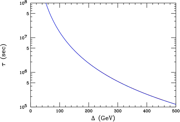
Figure 1: Lifetime for the decay $B_{1\pm 1}\rightarrow G_{1\pm 1}\gamma$ as a function of the mass splitting, for $M_{G}=3-5$ TeV. Note that the $M_{G}$ mass dependence within the thickness of the curve cannot be resolved over the plot’s range.

Other gravitationally induced lifetimes can be obtained in a similar fashion with qualitatively similar results.

IV Collider Signatures

The next questions to address are ($i$) can we see the physics associated with this $S^{2}$ picture and ($ii$) can we differentiate the present model from, e.g., the more conventional scenarios such as $S^{1}/Z_{2}$ and $T^{2}/Z_{2}$? To answer them we must be able to directly observe the KK excitations of the various SM gauge bosons at the LHC. Except for possible kinematic limitations, the resonant $m=0$ KK states should be accessible in a straightforward manner. The observation of pair produced KK states seems to be very unlikely due to their large masses which greatly suppress their production cross sectionspairs even at LHC energies.

The resonant neutral electroweak KK states can be produced in the Drell-Yan channel $q\bar{q}\rightarrow X\rightarrow l^{+}l^{-}$; here $X$ includes the SM zero modes $\gamma$ and $Z$ as well as all of the kinematically accessible KK states colliders . In the discussion that follows we will assume that all of the SM fermions are located at either the North or South Poles of the sphere, i.e., have either $\theta=0$ or $90^{o}$ but not both.

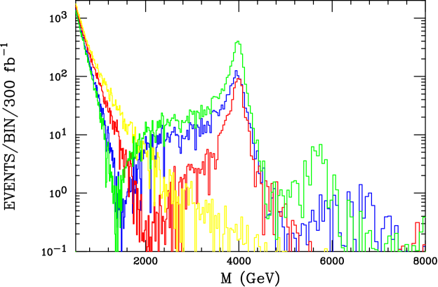
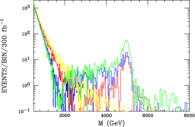
Figure 2: Drell-Yan production rate as a function of the dilepton pair invariant mass of the neutral electroweak KK resonances at the LHC. The upper(lower) plot corresponds to the case where the lightest KK has a mass of 4(5) TeV. The yellow histogram in both panels is the SM background while the blue(red,green) histogram corresponds to the case of $S^{2}(S^{1}/Z_{2},T^{2}/Z_{2})$. Fermions are assumed to be completely localized at either the North or South Poles. The bin size is $1\%$ of the dilepton invariant mass.

Fig. 2 shows the case where the lightest KK mass is assumed to be 4 or 5 TeV. For either mass value the degenerate KK resonance structure due to the simultaneous production of the states $(B,W^{0})_{10}$ can be observed above the SM backgrounds. At first glance looking at the Figure, this may not appear to be the case. However, we must remember that these are binned distributions. For example, in the case of $M=4$ TeV, if we make a cut of 2 TeV on the minimum dilepton pair mass we find 96 SM induced background events and 1670(763,4007) signal events in the case of the $S^{2}(S^{1}/Z_{2},T^{2}/Z_{2})$ model. In the case of $M=5$ TeV, there would be 1454(309,1717) signal events for these two models. There is thus no question of the presence of a signal in all cases.

Comparing, $S^{2}$ with $S^{1}/Z_{2}$, due to the larger couplings, the resonance structure of the $S^{2}$ case is significantly broader and the well-known colliders KK destructive interference minimum occurs at a significantly lower value of the dilepton invariant mass. $T^{2}/Z_{2}$ is also distinctive due to both the double degeneracy of the first KK level, which produces a generally larger cross section, and the relatively low mass of the second KK excitation. These differences are all clearly visible in the 4 TeV case but are somewhat harder to observe in the case where the first KK state has a mass of 5 TeV assuming an integrated luminosity of 300 $fb^{-1}$. Unlike in the $T^{2}/Z_{2}$ scenario, in either mass case for $S^{2}$ or $S^{1}/Z_{2}$ it is unlikely that any higher resonances due to more massive KK states would be observed. This situation improves significantly if we consider the luminosity upgrade of the LHC Gianotti:2002xx as shown in Fig. 3. Here we see that if the first $S^{2}$ KK mass lies at 4 TeV, it may be possible with higher luminosity to observe the degenerate $(B,W^{0})_{20}$ structure at a mass of $\simeq 6.93$ TeV, which is predicted to be more massive, i.e., 8 TeV in the case of the $S^{1}/Z_{2}$ scenario. For the $T^{2}/Z_{2}$ scenario, the second KK state lies at $\simeq 5.66$ TeV and is easily visible even at the lower luminosity. This further aids in distinguishing the three models. It is clear that at higher luminosities, the lightest KK states may be observable up to $\simeq 7$ TeV or more for all classes of models.

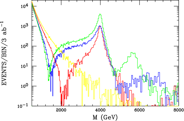
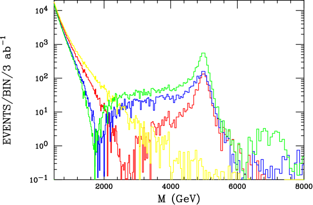
Figure 3: Same as the previous figure but now for the LHC upgrade with an order of magnitude higher integrated luminosity.

In order to help verify that any new resonances observed at the LHC are due to the production of KK excitations of the SM gauge fields, it is necessary to see their production in several channels. In addition to the $q\bar{q}\rightarrow(B,W^{0})_{l0}\rightarrow l^{+}l^{-}$ channel discussed above, the lightest of the corresponding $W^{\pm}_{l0}$ states should also be observed via the process $q\bar{q}^{\prime}\rightarrow W^{\pm}_{l0}\rightarrow l^{\pm}+E_{T}^{miss}$ colliders . Fig. 4 shows the transverse mass distribution for the lepton plus missing $E_{T}$ final state induced by the production of these charged states at the LHC. It is clear from this Figure that the direct production of these states should most likely be visible out to $\simeq 6$ TeV in this channel and that $S^{2}-S^{1}/Z_{2}$ model differentiation is possible for masses up to approximately 5 TeV. Differentiation of $S^{2}$ and $T^{2}/Z_{2}$ is seen to be significantly more difficult in this channel even with the high integrated luminosities assumed here.

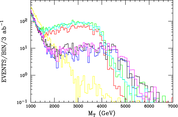
Figure 4: Transverse mass distributions for $W^{\pm}_{l0}$ production at the LHC. The lowest, steeply falling histogram is the SM background. The top(lower) triplet of signal histograms is for a lightest $W^{\pm}_{10}$ KK mass of 4(5) TeV. The upper(middle,lower) member of each pair is for the $T^{2}/Z_{2}$($S^{2}$,$S^{1}/Z_{2}$)model.

KK signatures can also be observed in other channels associated with the gluon KK excitations $g_{l0}$. Fig. 5 shows the dijet mass spectrum at the LHC subject to a pair of selection cuts for centrally produced objects. Here, we see that the existence of gluon KK excitations does not produce a significant resonance structure, except in the $T^{2}/Z_{2}$ case where there is added constructive interference from the degenerate pair of KK states. This is due to the fact that these resonances are rather wide and their relative cross sections, being in the $q\bar{q}$ channel, are relatively suppressed. Instead, one generally sees a rather broad shoulder induced by the existence of these KK states. For all of these models this shoulder should be observable for gluon KK masses in excess of 7 TeV. In the specific case where the lightest gluon KK mass is 4 TeV, the height of this shoulder is seen to be significantly different for the $S^{2}$ and $S^{1}/Z_{2}$ models allowing them to be easily distinguished. It remains difficult in this channel to distinguish the $S^{2}$ and $T^{2}/Z_{2}$ models away from the peak region. However, we note that, e.g., a 5 TeV KK in the $S^{1}/Z_{2}$ model produces a signal which is quite similar to a 7 TeV KK in the $S^{2}$ case. Thus, in general, since there is no obvious resonance structure for the $S^{2}$ and $S^{1}/Z_{2}$ models, they are only distinguishable in this channel if the mass of the lightest KK excitation is already known from other measurements such as the Drell-Yan channel discussed above.

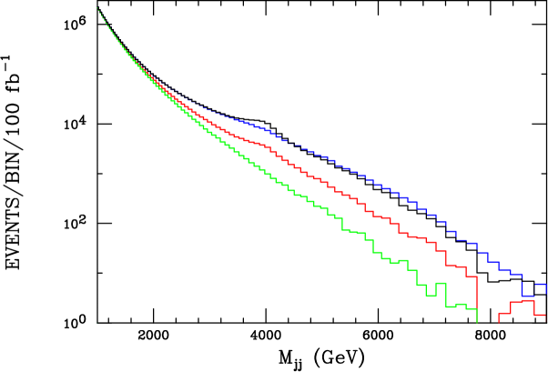
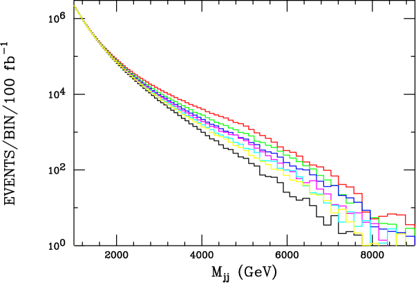
Figure 5: Dijet pair mass at the LHC applying the cut $|\eta|\leq 1$ and $p_{Tj}\geq 0.4M_{jj}$. The lowest histogram in both panels is the SM QCD background. In the top panel, a $g_{10}$ mass of 4 TeV has been assumed with the upper(middle,lower) signal histogram corresponding, on the right-hand side of the figure, to the $S^{2}(T^{2}/Z_{2},S^{1}/Z_{2})$ model. In the lower panel the top(middle) three histograms are for the $S^{2}(S^{1}/Z_{2})$ model assuming, from top to bottom, KK masses of 5, 6 or 7 TeV, respectively. Couplings between the KK states and SM zero mode gluons have been neglected.

Mixing between the SM zero mode gluon and the corresponding $m=0$ gluon KK excitations, while inducing a $ggg_{l0}$ coupling, does not alter these results in any significant way since the induced coupling is quite small being of order $\sim g_{4s}^{3}log^{2}(\Lambda R)/128\pi^{3}$. Even though the $gg$ luminosity is generally larger than $q\bar{q}$ luminosity, it cannot compensate at such large $x$ values for the rather strongly suppressed loop-induced $ggg_{l0}$ coupling; this is especially true at larger dijet masses which are relevant here.

From the above discussion, it is clear that the KK states of interest will be visible in all resonant channels and that the $S^{2}$ model of interest to us here can be differentiated from both the $S^{1}/Z_{2}$ and $T^{2}/Z_{2}$ model cases provided that the mass scale for these states is not too large.

V Conclusions

In this work, we studied a scenario in which the SM gauge and possibly Higgs sectors propagate in compact spherical extra dimensions. Since spheres $S^{n}$ do not allow chiral zero modes for fermions, these particles are naturally assumed to be localized at the poles and remain 4-dimensional in this scenario. The fermions can then lead to the appearance of pole localized kinetic terms for the gauge sector, which can result in level mixing among the “non-magnetic” ($m=0$) KK modes.

We focused on $S^{2}$ as a simple representative case and analyzed the vector KK towers of the gauge sector. We found that the symmetries of the geometry result in the appearance of certain KK gauge fields that may be stable. This picture can change once KK gravitons are assumed to be the be lightest states, level by level, as they are expected to receive suppressed quantum corrections to their masses. In that case, the previously stable states can decay into KK gravitons with macroscopically long lifetimes. Other gauge KK modes can decay into SM fermions which are localized at poles, and hence such states may be produced as resonances at the LHC.

Current precision electroweak bounds push the mass of the the first KK mode to about 4 TeV. However, we have shown that a 4-5 TeV KK mode is well within the reach of the LHC. The features of these resonances are quite distinct from their toroidal ($S^{1}/Z_{2}$ and $T^{2}/Z_{2}$) counterparts. A luminosity-upgraded LHC with 3 ab^-1 delivered can potentially access the second KK excitations of the SM gauge fields and establish the characteristic mass ratios special to $S^{2}$.

In general, we find that the gauge KK resonances on $S^{2}$ can be distinguished from those of other compactifications, such as $S^{1}/Z_{2}$ and $T^{2}/Z_{2}$, by the ratios of KK masses, the growing strength of the couplings of the KK fields to pole localized SM fermions, and the size of the production cross section. In particular, the lightest KK mode on $S^{2}$ couples to SM fermions with enhanced strength compared to its $S^{1}/Z_{2}$ counterpart. This feature affects the shape of the KK resonance in all the channels we examined. The first $T^{2}/Z_{2}$ KK mode has the largest production cross section of all three cases, due to double degeneracy. The second KK mode is lightest in the $T^{2}/Z_{2}$, and heaviest in the $S^{1}/Z_{2}$ case, given the same compactification radius.

In summary, we showed that the properties of spherical extra dimensions are qualitatively different from the more familiar toroidal ones. These new features can lead to the emergence of alternative models and open novel avenues for phenomenological studies.

- (1) L. Randall and R. Sundrum, Phys. Rev. Lett. 83, 3370 (1999) [arXiv:hep-ph/9905221].
- (2) F. Leblond, Phys. Rev. D 64, 045016 (2001) [arXiv:hep-ph/0104273].
- (3) C. S. Lim, N. Maru and K. Hasegawa, arXiv:hep-th/0605180.
- (4) R. Camporesi and A. Higuchi, J. Geom. Phys. 20, 1 (1996) [arXiv:gr-qc/9505009].
- (5) A. A. Abrikosov, Int. J. Mod. Phys. A 17, 885 (2002) [arXiv:hep-th/0111084].
- (6) t. L. E. Group [OPAL Collaboration], arXiv:hep-ex/0612034.
- (7) I. Antoniadis, Phys. Lett. B 246, 377 (1990); I. Antoniadis, C. Munoz and M. Quiros, Nucl. Phys. B 397, 515 (1993) [arXiv:hep-ph/9211309]; I. Antoniadis, S. Dimopoulos, A. Pomarol and M. Quiros, Nucl. Phys. B 544, 503 (1999) [arXiv:hep-ph/9810410]; A. Delgado, A. Pomarol and M. Quiros, Phys. Rev. D 60, 095008 (1999) [arXiv:hep-ph/9812489]; R. Barbieri, L. J. Hall and Y. Nomura, Phys. Rev. D 63, 105007 (2001) [arXiv:hep-ph/0011311].
- (8) I. Antoniadis, K. Benakli and M. Quiros, Phys. Lett. B 331, 313 (1994) [arXiv:hep-ph/9403290]; P. Nath, Y. Yamada and M. Yamaguchi, Phys. Lett. B 466, 100 (1999) [arXiv:hep-ph/9905415]; T. G. Rizzo, AIP Conf. Proc. 530, 290 (2000) [arXiv:hep-ph/9911229]. and Phys. Rev. D 61, 055005 (2000) [arXiv:hep-ph/9909232]; G. Polesello and M. Prata, Eur. Phys. J. C 32S2, 55 (2003); G. Azuelos and G. Polesello, Eur. Phys. J. C 39S2, 1 (2005). G. Azuelos et al., Eur. Phys. J. C 3̱9S2, 13 (2005) [arXiv:hep-ph/0402037]; T. G. Rizzo, in Proc. of the APS/DPF/DPB Summer Study on the Future of Particle Physics (Snowmass 2001) ed. N. Graf, In the Proceedings of APS / DPF / DPB Summer Study on the Future of Particle Physics (Snowmass 2001), Snowmass, Colorado, 30 Jun - 21 Jul 2001, pp P304 [arXiv:hep-ph/0109179]; E. Accomando and K. Benakli, arXiv:hep-ph/0512243; M. Escalier, Czech. J. Phys. 54, A269 (2004); S. J. Huber, C. A. Lee and Q. Shafi, Phys. Lett. B 531, 112 (2002) [arXiv:hep-ph/0111465]; T. G. Rizzo, in Proc. of the APS/DPF/DPB Summer Study on the Future of Particle Physics (Snowmass 2001) ed. N. Graf,In the Proceedings of APS / DPF / DPB Summer Study on the Future of Particle Physics (Snowmass 2001), Snowmass, Colorado, 30 Jun - 21 Jul 2001, pp P302 [arXiv:hep-ph/0108234]; D. A. Dicus, C. D. McMullen and S. Nandi, Phys. Rev. D 66, 010001 (2002) arXiv:hep-ph/0012259.
- (9) J. L. Feng, A. Rajaraman and F. Takayama, Phys. Rev. D 68, 085018 (2003) [arXiv:hep-ph/0307375].
- (10) T. Appelquist, H. C. Cheng and B. A. Dobrescu, Phys. Rev. D 64, 035002 (2001) [arXiv:hep-ph/0012100]; H. C. Cheng, K. T. Matchev and M. Schmaltz, Phys. Rev. D 66, 056006 (2002) [arXiv:hep-ph/0205314] and Phys. Rev. D 66, 036005 (2002) [arXiv:hep-ph/0204342].
- (11) See, for example, the discussion in: C. E. Carlson and C. D. Carone, Phys. Rev. D 65, 075007 (2002) [arXiv:hep-ph/0112143].
- (12) N. Arkani-Hamed, S. Dimopoulos and G. R. Dvali, Phys. Lett. B 429, 263 (1998) [arXiv:hep-ph/9803315]; I. Antoniadis, N. Arkani-Hamed, S. Dimopoulos and G. R. Dvali, Phys. Lett. B 436, 257 (1998) [arXiv:hep-ph/9804398]; N. Arkani-Hamed, S. Dimopoulos and G. R. Dvali, Phys. Rev. D 59, 086004 (1999) [arXiv:hep-ph/9807344].
- (13) M. Carena, T. M. P. Tait and C. E. M. Wagner, Acta Phys. Polon. B 33, 2355 (2002) [arXiv:hep-ph/0207056]; M. Carena, E. Ponton, T. M. P. Tait and C. E. M. Wagner, Phys. Rev. D 67, 096006 (2003) [arXiv:hep-ph/0212307]; H. Davoudiasl, J. L. Hewett and T. G. Rizzo, Phys. Rev. D 68, 045002 (2003) [arXiv:hep-ph/0212279]; F. del Aguila, M. Perez-Victoria and J. Santiago, JHEP 0302, 051 (2003) [arXiv:hep-th/0302023].
- (14) For a discussion of these effects with toroidal extra deimensions, see the third paper in Ref. ued .
- (15) T. G. Rizzo and J. D. Wells, Phys. Rev. D 61, 016007 (2000) [arXiv:hep-ph/9906234]; K. m. Cheung and G. Landsberg, Phys. Rev. D 65, 076003 (2002) [arXiv:hep-ph/0110346]; A. Strumia, Phys. Lett. B 466, 107 (1999) [arXiv:hep-ph/9906266]; A. Delgado, A. Pomarol and M. Quiros, JHEP 0001, 030 (2000) [arXiv:hep-ph/9911252]; F. Cornet, M. Relano and J. Rico, Phys. Rev. D 61, 037701 (2000) [arXiv:hep-ph/9908299]; C. D. Carone, Phys. Rev. D 61, 015008 (2000) [arXiv:hep-ph/9907362]; P. Nath and M. Yamaguchi, Phys. Rev. D 60, 116004 (1999) [arXiv:hep-ph/9902323]; A. Muck, A. Pilaftsis and R. Ruckl, Phys. Rev. D 65, 085037 (2002) [arXiv:hep-ph/0110391].
- (16) J. Kang, M. A. Luty and S. Nasri, arXiv:hep-ph/0611322; C. Bambi, A. D. Dolgov and K. Freese, arXiv:hep-ph/0612018.
- (17) T. G. Rizzo, Phys. Rev. D 64, 095010 (2001) [arXiv:hep-ph/0106336]; D. A. Dicus, C. D. McMullen and S. Nandi, Phys. Rev. D 65, 076007 (2002) [arXiv:hep-ph/0012259].
- (18) F. Gianotti et al., Eur. Phys. J. C 39, 293 (2005) [arXiv:hep-ph/0204087].