Parton distribution function for quarks in an $s$-channel approach

Abstract

We use an $s$-channel picture of hard hadronic collisions to investigate the parton distribution function for quarks at small momentum fraction $x$, which corresponds to very high energy scattering. We study the renormalized quark distribution at one loop in this approach. In the high-energy picture, the quark distribution function is expressed in terms of a Wilson-line correlator that represents the cross section for a color dipole to scatter from the proton. We model this Wilson-line correlator in a saturation model. We relate this representation of the quark distribution function to the corresponding representation of the structure function $F_{T}(x,Q^{2})$ for deeply inelastic scattering.

I Introduction

Proton structure at large $Q^{2}$ and small Bjorken $x$ has been extensively investigated in experiments at HERA. This program is of great intrinsic interest and provides valuable information for the LHC program, where the short-distance structure of protons and nuclei will be probed at TeV energies. Two physical pictures that seem very different from each other are used to analyze hadronic structure functions for large $Q^{2}$ and small $x$.

There is a parton picture, in which the hadron consists of partons and the partons undergo a hard collision that produces the final state. This is reviewed in jjj . This applies at large $Q^{2}$. The corresponding theoretical method is that of factorization. The cross section is written as a convolution of parton distribution functions, $f_{a/A}(x,Q^{2})$, and a hard cross section for partonic scattering. The parton distribution functions are evaluated at small $x$, but the $x$ dependence is not predicted except insofar as it results from evolution starting from $f_{a/A}(x,Q_{0}^{2})$ at a smaller virtuality scale $Q_{0}^{2}$.

There is an $s$-channel picture, in which one thinks of the event in the rest frame of one of the hadrons. See ericemue for recent accounts. This applies at small $x$. The hard interaction takes place far outside the hadron and the products of the interaction travel toward the hadron and interact with it. In the simplest case, there are effectively two objects that collide with the hadron. These objects carry opposite color, so that they can be said to constitute a “color dipole”, described by a correlator of two eikonal Wilson lines. An important concept here is that the cross section for the color dipole to scatter from the hadron can be simple when the transverse separation between the elements of the dipole are large. Then the dipole always scatters as long as its impact parameter is within the hadron radius. One speaks of the cross section saturating – that is, being as large as it possibly could be golecrev ; mue99 .

These pictures seem quite different, as they look at the collision in different reference frames, and lead to different theoretical methods, but they are not at all incompatible. In the region where their domains of validity overlap, they must describe the same physics. The aim of this paper is to connect the two pictures.

We examine one of the main ingredients used in the parton picture, namely the distribution function for finding a quark in a hadron, defined as a hadronic matrix element of a certain product of operators cs82 . For very small $x$, the parton system created by this operator is far outside the hadron. We analyze the evolution of the system using $s$-channel methods. We find that the quark distribution can be expressed as a Wilson-line correlator convoluted with a simple lightcone wave function. Moreover, we find that this answer allows one to relate with precision the seemingly dissimilar results for structure functions in the parton framework and the $s$-channel framework.

Part of the results of this analysis have been used in plb06 to investigate the power corrections to structure functions that arise from the $s$-channel picture.

The content of the paper is as follows. We begin by applying the hamiltonian method hks to the quark distribution function. This allows us to write the quark distribution as a convolution of a lightcone wave function and a matrix element of eikonal-line operators (Sec. II). We work in the lowest-order approximation, i.e., the dipole approximation. The convolution formula provides a simple interpretation in coordinate space for the physical process that probes the distribution. The parton distribution is defined by matrix elements of operator products that require renormalization. We perform the renormalization at one loop using the $\overline{\rm MS}$ subtraction scheme for the ultraviolet divergences.

The eikonal-operator matrix element receives contribution from both short distances and long distances. We first analyze it by an expansion in powers of $gA$ (with $g$ the strong coupling and $A$ the gauge field), valid at short distances (Sec. III). This expansion is useful to carry out the matching with renormalization-group evolution equations. In particular, it allows us to relate the eikonal matrix element at short distances to a well-prescribed integral of the gluon distribution function.

Next, we motivate and discuss a widely used approach for modeling the eikonal-operator matrix element at large distances (Sec. IV), based on parton saturation golecrev ; mue99 . As the saturation scale in the quark sector is likely to be at much lower momenta than in the gluon sector (see e.g. hs00 ), we critically examine the validity of the treatment for the quark distribution, and the potential breakdown of the dipole approximation (Sec. V).

We finally discuss the relation of our results for the quark distribution with known dipole results for structure functions (Sec. VI). This discussion also illustrates how standard factorization properties are reobtained from the $s$-channel point of view.

Some supplementary material is left to the appendices. In Appendix A we collect calculational details on integrals of lightcone wave functions. In Appendix B we give a relation between products of eikonal operators for color-octet and color-triplet dipoles. In Appendix C we report details on applying the hamiltonian method to the hadronic matrix element of two currents.

II Quark distribution in the s-channel picture

We study the quark distribution using the $s$-channel picture in the style of hks . We start with the definition cs82 of the quark distribution as a proton matrix element of a certain operator,

$$f_{q/p}(x,\mu) = {1\over 4\pi}\left({1\over 2}\sum_{s}\right)\int\!dy^{-}e^{ixP^{+}y^{-}}$$ (1)

$$\times\langle P,s|\bar{\psi}(0)Q(0)\gamma^{+}Q^{\dagger}(y^{-})\psi(0,y^{-},{\bm{0}})|P,s\rangle_{c}.$$

Here for any four-vector $z^{\mu}$ we use lightcone components $z^{\pm}$ defined as

$$z^{\pm}={{z^{0}\pm z^{3}}\over\sqrt{2}}\;.$$ (2)

The proton momentum is

$$P=\left(P^{+},P^{-},P_{\perp}\right)=\left(P^{+},\frac{M_{p}^{2}}{2P^{+}},{\bm{0}}\right)\;.$$ (3)

The operator $Q^{\dagger}$ is the path-ordered exponential of the color potential

$$Q^{\dagger}(y^{-})={\cal P}\exp\left\{-ig\int_{y^{-}}^{+\infty}dz^{-}{A}^{+}_{a}(0,z^{-},{\bm{0}})t_{a}\right\}\;,$$ (4)

where the path ordering instruction ${\cal P}$ puts fields and color matrices with the most positive values of $z^{-}$ to the left. Equivalently, following the notation of hks , we can think of $Q^{\dagger}(y^{-})$ as creating an eikonal particle that moves in the minus direction, starting at minus coordinate $y^{-}$. An eikonal particle is an imaginary particle that retains its plus and transverse positions no matter how much momentum it absorbs. The subscript $c$ on the matrix element in Eq. (1) indicates that we are to take the connected parts of the graphs, in which some partons from the proton states communicate with the indicated operators. The operator product in Eq. (1) is ultraviolet divergent and requires renormalization. We will use the standard $\overline{\rm MS}$ prescription. The required subtraction at the one loop level is analyzed in Sec. II.5.

II.1 The quark distribution as a forward scattering amplitude

We begin by rewriting the matrix element in Eq. (1) so that it has the form of the real part of a forward scattering amplitude. To do this, we write $f_{q/p}(x,\mu)$ in two pieces,

$$f_{q/p}(x,\mu)=f^{+}_{q/p}(x,\mu)+f^{-}_{q/p}(x,\mu),$$ (5)

where

$$f^{+}_{q/p}(x,\mu) = {1\over 4\pi}\left({1\over 2}\sum_{s}\right)\int_{0}^{\infty}\!dy^{-}e^{ixP^{+}y^{-}}$$ (6)

$$\times\langle P,s|\bar{\psi}(0)Q(0)\gamma^{+}Q^{\dagger}(y^{-})\psi(0,y^{-},{\bm{0}})|P,s\rangle_{c}$$

and

$$f^{-}_{q/p}(x,\mu) = {1\over 4\pi}\left({1\over 2}\sum_{s}\right)\int^{0}_{-\infty}\!dy^{-}e^{ixP^{+}y^{-}}$$ (7)

$$\times\langle P,s|\bar{\psi}(0)Q(0)\gamma^{+}Q^{\dagger}(y^{-})\psi(0,y^{-},{\bm{0}})|P,s\rangle_{c}.$$

We note that

$$f^{+}_{q/p}(x,\mu)=[f^{-}_{q/p}(x,\mu)]^{*}.$$ (8)

Thus $f$ is twice the real part of $f^{-}$:

$$f_{q/p}(x,\mu) = {\rm Re}\,{1\over 2\pi}\left({1\over 2}\sum_{s}\right)\int_{-\infty}^{0}\!dy^{-}e^{ixP^{+}y^{-}}$$ (9)

$$\times\langle P,s|T\!\left\{\bar{\psi}(0)Q(0)\gamma^{+}Q^{\dagger}(y^{-})\psi(0,y^{-},{\bm{0}})\right\}|P,s\rangle_{c}.$$

The operator product in $f^{-}$ is time ordered since $y^{-}<0$. The $T$ here indicates this time ordering. For our purposes, it is helpful to insert a factor $x$ and another $y^{-}$ integral:

$$xf_{q/p}(x,\mu)=$$ (10)

$${\rm Re}\,{2xP^{+}\over 2\pi}\left({1\over 2}\sum_{s}\right)\int\!dy_{2}^{-}dy_{1}^{-}\ \theta(y_{2}^{-}>y_{1}^{-})e^{-ixP^{+}(y_{2}^{-}-y_{1}^{-})}\int\frac{dP^{\prime+}}{(2\pi)2P^{\prime+}}$$

$$\times\langle P^{\prime},s|T\!\left\{\bar{\psi}(0,y_{2}^{-},{\bm{0}})Q(y_{2}^{-})\gamma^{+}Q^{\dagger}(y_{1}^{-})\psi(0,y_{1}^{-},{\bm{0}})\right\}|P,s\rangle_{c}.$$

The integral over $P^{\prime+}$ can be thought of as setting the proton state to position $y^{-}=0$. We have thus rewritten the original $f$, which was analogous to a total cross section, as a Green function analogous to a forward scattering amplitude. Our next task is to break the scattering amplitude into parts that can be analyzed separately.

II.2 Decomposition of the gluon field

The Fourier transformed operator $Q^{\dagger}(y_{1}^{-})\psi(0,y_{1}^{-},{\bm{0}})$ in Eq. (10) creates an antiquark and an eikonal particle with a total plus-momentum $xP^{+}$. We consider that $x$ is very small, say $10^{-3}$. That means that the typical distance $y_{1}^{-}$ from the proton to where the antiquark and the eikonal particle are created is large, of order $1/(xP^{+})$. This is way outside the proton. The antiquark and eikonal particle develop into a shower of partons with minus-momenta of order $k^{-}=(k_{\perp}^{2}+k^{2})/(2k^{+})\sim m^{2}/(xP^{+})$, where $k_{\perp}$ is the transverse momentum of the parton and $k^{2}$ is its virtuality and we take both of these to be of order $m^{2}\equiv(300\ {\rm MeV})^{2}$. Thus the partons created by the original operator have very large minus-momenta. We will speak of them as “fast” partons. As noted, the fast partons travel a long distance in $y^{-}$ before meeting the proton.

When the fast partons meet the proton, they scatter from the gluon field of the proton, as depicted in Fig. 1. The gluon field of the proton consists of “slow” gluons, with plus-momenta much larger than $xP^{+}$. (Then the minus-momenta of these gluons, $k^{-}=(k_{\perp}^{2}+k^{2})/(2k^{+})$ is much smaller than $m^{2}/(xP^{+})$, assuming again that $k_{\perp}^{2}$ and $k^{2}$ are of order $m^{2}$.) We represent the gluon field produced by the proton as an external field ${\cal A}^{\mu}(x)$ and consider the quantity

$$U[{\cal A}] = {2xP^{+}\over 2\pi}\int\!dy_{2}^{-}dy_{1}^{-}e^{-ixP^{+}(y_{2}^{-}-y_{1}^{-})}$$ (11)

$$\times\left\{\langle 0|\bar{\psi}(0,y_{2}^{-},{\bm{0}})Q(y_{2}^{-})\gamma^{+}Q^{\dagger}(y_{1}^{-})\psi(0,y_{1}^{-},{\bm{0}})|0\rangle_{\cal A}\right.$$

$$\quad-\left.\langle 0|\bar{\psi}(0,y_{2}^{-},{\bm{0}})Q(y_{2}^{-})\gamma^{+}Q^{\dagger}(y_{1}^{-})\psi(0,y_{1}^{-},{\bm{0}})|0\rangle_{0}\right\}.$$

This is the amplitude for the fast partons to be created by the operator $Q^{\dagger}\psi$, scatter from the external field ${\cal A}$, then be annihilated by the conjugate operator $\bar{\psi}Q$. In the second term, we subtract a no-scattering term with the external field set to zero, in accordance with the instruction to take only connected graphs. Then the quark distribution is a proton matrix element of $U[A]$, with the external field ${\cal A}$ replaced by the quantum field $A$,

$$xf_{q/p}(x,\mu)={\rm Re}\,\left({1\over 2}\sum_{s}\right)\int\frac{dP^{\prime+}}{(2\pi)2P^{\prime+}}\langle P^{\prime},s|U[A]|P,s\rangle.$$ (12)

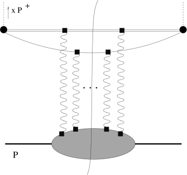
Figure 1: Quark distribution in the $s$-channel picture. The black circles at the top represent the insertion of the operators in Eq. (10). The double straight line represents the eikonal. Any number of slow gluons couple the fast parton and the eikonal to the proton.

There is, of course, a catch in this. There is only one gluon field $A^{\mu}(x)$. We need to divide it into two pieces, one associated with the fast partons and one associated with the proton. To do this, we choose a momentum fraction $x_{c}$. Gluons with plus-momenta smaller than $x_{c}P^{+}$ are associated with the fast partons. Gluons with plus-momenta larger than $x_{c}P^{+}$ are associated with the proton and included in the external field ${\cal A}$ in Eq. (11). In order for the approximations discussed below to work, we need $x\ll x_{c}$. It is perhaps easiest to think about the physics taking $x_{c}$ to be of order $1/(R_{p}P^{+})$, so that the proton’s field is considered to have a spatial extent of the order of the proton radius, $R_{p}$. However, in the end we will want to take $x_{c}\ll 1$ and in fact let $x_{c}$ be pretty close to $x$.

We will, in fact, not need to be very specific about how to implement the division at momentum fraction $x_{c}$. For our discussion of the quark distribution, working at lowest order in perturbation theory, we are saved from sensitivity to the splitting method by the fact that the $g\to q\bar{q}$ Altarelli-Parisi splitting function does not have a soft singularity. If we worked with the gluon distribution or with the quark distribution to higher order, we would need a more sophisticated analysis.

II.3 The evolution operator $U$ at high energy

The function $U[{\cal A}]$ can be written in the interaction picture with ${\cal A}$ as the perturbation:

$$U[{\cal A}] = {2xP^{+}\over 2\pi}\int\!dy_{2}^{-}dy_{1}^{-}\theta(y_{2}^{-}-y_{1}^{-})\,e^{-ixP^{+}(y_{2}^{-}-y_{1}^{-})}$$ (13)

$$\times\langle 0|U(\infty,y_{2}^{-})\bar{\psi}(0,y_{2}^{-},{\bm{0}})Q(y_{2}^{-})\gamma^{+}$$

$$\times\ \ \ \ U(y_{2}^{-},y_{1}^{-})Q^{\dagger}(y_{1}^{-})\psi(0,y_{1}^{-},{\bm{0}})U(y_{1}^{-},\infty)|0\rangle$$

$$-({\rm same\ with\ }{\cal A}=0).$$

This is without approximation. Now we recognize that for small $x$, only $y_{2}^{-}\gg r^{-}$ and $y_{1}^{-}\ll-r^{-}$ are important, where $r^{-}$ is the effective radius of the proton’s field in the longitudinal direction, $r^{-}=1/(x_{c}P^{+})$. The external field is concentrated in $|y^{-}|<r^{-}$, so we have

$$U[{\cal A}] \approx {2xP^{+}\over 2\pi}\int_{0}^{\infty}\!dy_{2}^{-}\int_{-\infty}^{0}\!dy_{1}^{-}e^{-ixP^{+}(y_{2}^{-}-y_{1}^{-})}$$ (14)

$$\times\langle 0|\bar{\psi}(0,y_{2}^{-},{\bm{0}})Q(y_{2}^{-})\gamma^{+}[U(\infty,-\infty)-1]Q^{\dagger}(y_{1}^{-})\psi(0,y_{1}^{-},{\bm{0}})|0\rangle.\ \ \ \$$

Here we have subtracted the no-scattering term as “$-1$”.

At this stage, our quantum fields are evolving with full QCD [not including the external field, which is represented in $U(\infty,-\infty)$]. Let us now expand this evolution in powers of $\alpha_{s}$ and take just the Born term. Then the fields evolve with just the free field hamiltonian. We can insert intermediate states, and at this level of approximation, the intermediate states contain just one antiquark and the one eikonal particle ${\cal E}$. We get

$$U[{\cal A}] \approx {2xP^{+}\over 2\pi}\int_{0}^{\infty}\!dy_{2}^{-}\int_{-\infty}^{0}\!dy_{1}^{-}e^{-ixP^{+}(y_{2}^{-}-y_{1}^{-})}$$ (15)

$$\times(2\pi)^{-6}\int_{0}^{\infty}\!{dp_{2}^{-}\over 2p_{2}^{-}}\int\!d{\bm{p}}_{2}\int_{0}^{\infty}\!{dp_{1}^{-}\over 2p_{1}^{-}}\int\!d{\bm{p}}_{1}\sum_{s_{1}s_{2}}$$

$$\times\langle 0|\bar{\psi}(0,y_{2}^{-},{\bm{0}})Q(y_{2}^{-})\gamma^{+}|p_{2}^{-},{\bm{p}}_{2},s_{2},{\cal E}\rangle$$

$$\times\langle p_{2}^{-},{\bm{p}}_{2},s_{2},{\cal E}|U(\infty,-\infty)-1|p_{1}^{-},{\bm{p}}_{1},s_{1},{\cal E}\rangle$$

$$\times\langle p_{1}^{-},{\bm{p}}_{1},s_{1},{\cal E}|Q^{\dagger}(y_{1}^{-})\psi(0,y_{1}^{-},{\bm{0}})|0\rangle.$$

Taking into account that particle 1 has plus momentum $p_{1}^{+}={\bm{p}}_{1}^{2}/(2p_{1}^{-})$ while particle 2 has plus momentum $p_{2}^{+}={\bm{p}}_{2}^{2}/(2p_{2}^{-})$, we can evaluate the dependence of the matrix elements on $y_{1}^{-}$ and $y_{2}^{-}$ as

$$U[{\cal A}] \approx {2xP^{+}\over(2\pi)^{7}}\int_{0}^{\infty}\!{dp_{2}^{-}\over 2p_{2}^{-}}\int\!d{\bm{p}}_{2}\int_{0}^{\infty}\!{dp_{1}^{-}\over 2p_{1}^{-}}\int\!d{\bm{p}}_{1}\sum_{s_{1}s_{2}}$$ (16)

$$\times\int_{0}^{\infty}\!dy_{2}^{-}\int_{-\infty}^{0}\!dy_{1}^{-}e^{-i(xP^{+}+p_{2}^{+})y_{2}^{-}}e^{+i(xP^{+}+p_{1}^{+})y_{1}^{-}}$$

$$\times\langle 0|\bar{\psi}(0)Q(0)\gamma^{+}|p_{2}^{-},{\bm{p}}_{2},s_{2},{\cal E}\rangle$$

$$\times\langle p_{2}^{-},{\bm{p}}_{2},s_{2},{\cal E}|U(\infty,-\infty)-1|p_{1}^{-},{\bm{p}}_{1},s_{1},{\cal E}\rangle$$

$$\times\langle p_{1}^{-},{\bm{p}}_{1},s_{1},{\cal E}|Q^{\dagger}(0)\psi(0)|0\rangle.$$

We can now perform the $y^{-}$ integrations to produce energy denominators:

$$U[{\cal A}] \approx {2xP^{+}\over(2\pi)^{7}}\int_{0}^{\infty}\!{dp_{2}^{-}\over 2p_{2}^{-}}\int\!d{\bm{p}}_{2}\int_{0}^{\infty}\!{dp_{1}^{-}\over 2p_{1}^{-}}\int\!d{\bm{p}}_{1}\sum_{s_{1}s_{2}}$$ (17)

$$\times{-i\over xP^{+}+p_{2}^{+}}\,{-i\over xP^{+}+p_{1}^{+}}$$

$$\times\langle 0|\bar{\psi}(0)Q(0)\gamma^{+}|p_{2}^{-},{\bm{p}}_{2},s_{2},{\cal E}\rangle$$

$$\times\langle p_{2}^{-},{\bm{p}}_{2},s_{2},{\cal E}|U(\infty,-\infty)-1|p_{1}^{-},{\bm{p}}_{1},s_{1},{\cal E}\rangle$$

$$\times\langle p_{1}^{-},{\bm{p}}_{1},s_{1},{\cal E}|Q^{\dagger}(0)\psi(0)|0\rangle.$$

For the factor giving the interaction of the partons with the external field, we have

$$\langle p_{2}^{-},{\bm{p}}_{2},s_{2},{\cal E}|U(\infty,-\infty)-1|p_{1}^{-},{\bm{p}}_{1},s_{1},{\cal E}\rangle=$$ (18)

$$\hskip 28.45274pt2\pi\,2p_{1}^{-}\,\delta(p_{1}^{-}-p_{2}^{-})\delta_{s_{1}s_{2}}[\tilde{F}({\bm{p}}_{1}-{\bm{p}}_{2})^{\dagger}F({\bm{0}})-(2\pi)^{2}\delta({\bm{p}}_{1}-{\bm{p}}_{2})],\ \$$

where

$$F({\bm{\Delta}})={\cal P}\exp\left\{-ig\int_{-\infty}^{+\infty}dz^{-}{\cal A}^{+}_{a}(0,z^{-},{\bm{\Delta}})t_{a}\right\}$$ (19)

and

$$\tilde{F}({\bm{k}})=\int d{\bm{\Delta}}\,e^{i{\bm{k}}\cdot{\bm{\Delta}}}F({\bm{\Delta}}).$$ (20)

This gives

$$U[{\cal A}]\approx\int d{\bm{\Delta}}\ \frac{1}{N_{c}}\,{\rm Tr}[1-F({\bm{\Delta}})^{\dagger}F({\bm{0}})]\ u({\bm{\Delta}}),$$ (21)

where

$$u({\bm{\Delta}}) = {4xP^{+}\over(2\pi)^{6}}\int_{0}^{\infty}\!dp^{-}\int\!d{\bm{p}}_{2}\int\!d{\bm{p}}_{1}\sum_{s}e^{i{\bm{\Delta}}\cdot({\bm{p}}_{1}-{\bm{p}}_{2})}$$ (22)

$$\times{p^{-}\over(2xP^{+}p^{-}+{\bm{p}}_{2}^{2})(2xP^{+}p^{-}+{\bm{p}}_{1}^{2})}$$

$$\times\langle 0|\bar{\psi}(0)Q(0)\gamma^{+}|p^{-},{\bm{p}}_{2},s,{\cal E}\rangle\langle p^{-},{\bm{p}}_{1},s,{\cal E}|Q^{\dagger}(0)\psi(0)|0\rangle.$$

Thus

$$xf_{q/p}(x,\mu)={\rm Re}\int d{\bm{\Delta}}\ u({\bm{\Delta}})\ \Xi_{I}({\bm{\Delta}}),$$ (23)

where

$$\Xi_{I}({\bm{\Delta}})=\left({1\over 2}\sum_{s}\right)\int\frac{dP^{\prime+}}{(2\pi)2P^{\prime+}}\langle P^{\prime},s|\frac{1}{N_{c}}\,{\rm Tr}[1-F({\bm{\Delta}})^{\dagger}F({\bm{0}})]|P,s\rangle.$$ (24)

Here $F({\bm{\Delta}})$ is now defined with the quantum field $A$,

$$F({\bm{\Delta}})={\cal P}\exp\left\{-ig\int_{-\infty}^{+\infty}dz^{-}A^{+}_{a}(0,z^{-},{\bm{\Delta}})t_{a}\right\}.$$ (25)

Eq. (23) has a simple interpretation. First, $u({\bm{\Delta}})$ is the square of the antiquark wave function, giving the probability that the antiquark has reached a separation $\bm{\Delta}$ from the eikonal line by the time it reaches the hadron. Second, we have a probability $\Xi_{I}({\bm{\Delta}})$ for the antiquark-eikonal dipole to scatter from the proton.

II.4 The squared wave function for the antiquark

We now need the function $u(\Delta)$. First, we need the operator matrix elements:

$$M \equiv \sum_{s}\langle 0|\bar{\psi}(0)Q(0)\gamma^{+}|p^{-},{\bm{p}}_{2},s,{\cal E}\rangle\langle p^{-},{\bm{p}}_{1},s,{\cal E}|Q^{\dagger}(0)\psi(0)|0\rangle$$ (26)

$$= \sum_{s}\langle 0|\bar{\psi}(0)\gamma^{+}|p^{-},{\bm{p}}_{2},s\rangle\langle p^{-},{\bm{p}}_{1},s|\psi(0)|0\rangle.$$

There is an implicit color trace here. Restoring the color indices makes it

$$M = \sum_{s}\langle 0|\bar{\psi}_{\alpha}(0)\gamma^{+}|p^{-},{\bm{p}}_{2},s,\beta\rangle\langle p^{-},{\bm{p}}_{1},s,\beta|\psi_{\alpha}(0)|0\rangle.$$ (27)

Writing this with spinors gives

$$M = \delta_{\alpha\beta}\delta_{\beta\alpha}\sum_{s}\bar{v}(p^{-},{\bm{p}}_{2},s)\gamma^{+}v(p^{-},{\bm{p}}_{1},s).$$ (28)

Now we need to know about the spin states. We use null-plane helicity states appropriate to the $x^{-}$ as the “time.” These have the normalization

$$\bar{v}(p^{-},{\bm{p}}_{2},s^{\prime})\gamma^{-}v(p^{-},{\bm{p}}_{1},s)=2p^{-}\delta_{ss^{\prime}}.$$ (29)

Thus

$$M = \delta_{\alpha\beta}\delta_{\beta\alpha}\sum_{ss^{\prime}}\bar{v}(p^{-},{\bm{p}}_{2},s)\gamma^{+}v(p^{-},{\bm{p}}_{1},s^{\prime})\delta_{ss^{\prime}}$$ (30)

$$= \frac{N_{c}}{2p^{-}}\sum_{ss^{\prime}}\bar{v}(p^{-},{\bm{p}}_{2},s)\gamma^{+}v(p^{-},{\bm{p}}_{1},s^{\prime})\ \bar{v}(p^{-},{\bm{p}}_{2},s^{\prime})\gamma^{-}v(p^{-},{\bm{p}}_{1},s)$$

$$= \frac{N_{c}}{2p^{-}}{\rm Tr}\{\hbox to0.0pt{/\hss}p_{1}\gamma^{-}\hbox to0.0pt{/\hss}p_{2}\gamma^{+}\}$$

$$= \frac{N_{c}}{2p^{-}}{\rm Tr}\{\hbox to0.0pt{/\hss}p_{1,T}\,\gamma^{-}\hbox to0.0pt{/\hss}p_{2,T}\,\gamma^{+}\}$$

$$= \frac{2N_{c}}{p^{-}}\ {\bm{p}}_{1}\cdot{\bm{p}}_{2}.$$

Thus

$$u({\bm{\Delta}}) = {2x\,2P^{+}\over(2\pi)^{6}}\int_{0}^{\infty}\!dp^{-}\int\!d{\bm{p}}_{2}\int\!d{\bm{p}}_{1}e^{i{\bm{\Delta}}\cdot({\bm{p}}_{1}-{\bm{p}}_{2})}$$ (31)

$$\times{p^{-}\over(2xP^{+}p^{-}+{\bm{p}}_{2}^{2})(2xP^{+}p^{-}+{\bm{p}}_{1}^{2})}$$

$$\times\frac{2N_{c}}{p^{-}}\ {\bm{p}}_{1}\cdot{\bm{p}}_{2}$$

$$= {4N_{c}\over(2\pi)^{6}}\int_{0}^{\infty}\!d\Lambda^{\!2}\int\!d{\bm{p}}_{2}\int\!d{\bm{p}}_{1}e^{i{\bm{\Delta}}\cdot({\bm{p}}_{1}-{\bm{p}}_{2})}$$

$$\times{{\bm{p}}_{1}\cdot{\bm{p}}_{2}\over(\Lambda^{\!2}+{\bm{p}}_{2}^{2})(\Lambda^{\!2}+{\bm{p}}_{1}^{2})},$$

where we have defined $\Lambda^{\!2}=2xP^{+}p^{-}$. Extending this to $4-2\epsilon$ dimensions, we have

$$u({\bm{\Delta}})={4N_{c}\mu^{4\epsilon}\over(2\pi)^{6-4\epsilon}}\int_{0}^{\infty}\!d\Lambda^{2}\int\!d^{2-2\epsilon}{\bm{p}}_{2}\int\!d^{2-2\epsilon}{\bm{p}}_{1}\ e^{i{\bm{\Delta}}\cdot({\bm{p}}_{1}-{\bm{p}}_{2})}\ {{\bm{p}}_{1}\cdot{\bm{p}}_{2}\over(\Lambda^{2}+{\bm{p}}_{2}^{2})(\Lambda^{2}+{\bm{p}}_{1}^{2})}.$$ (32)

We perform the integration separately in Appendix A. We find

$$u({\bm{\Delta}})={N_{c}\over 3\pi^{4}}\,\frac{1}{\Delta^{4}}\ \left(\pi\mu^{2}\Delta^{2}\right)^{2\epsilon}\frac{\Gamma(2-\epsilon)^{2}}{1-2\epsilon/3}.$$ (33)

II.5 Renormalization of the quark distribution

Using the result (33) for $u(\bm{\Delta})$, we have

$$xf_{q/p}(x,\mu)={N_{c}\over 3\pi^{4}}\ \frac{\Gamma(2-\epsilon)^{2}}{1-2\epsilon/3}\ \mu^{-2\epsilon}\!\int\!d^{2-2\epsilon}{\bm{\Delta}}\ {1\over\Delta^{4}}\,\left(\pi\mu^{2}\Delta^{2}\right)^{2\epsilon}\Xi_{I}({\bm{\Delta}})-{\rm{UV}}.$$ (34)

Here there is an ultraviolet divergence from the small $\Delta$ integration region. The notation indicates that we should renormalize the divergence by subtracting a UV counter term.

The standard definition of the parton distribution functions gives these functions as hadron matrix elements of operator products that must be renormalized cs82 . It is thus not a surprise that we have a divergent integral in Eq. (34). The standard treatment is to apply $\overline{\rm MS}$ renormalization. At the one loop level at which we work here, this means performing the integrals in $4-2\epsilon$ dimensions and subtracting a counter-term of the form

$${\rm``UV"}={\it const.}\times\frac{1}{\epsilon}\ \frac{(4\pi)^{\epsilon}}{\Gamma(1-\epsilon)}.$$ (35)

In this section, we implement this subtraction, turning it (approximately) into a cutoff on $|\bm{\Delta}|$.

We are eliminating only the divergence from the innermost loop in the Feynman diagrams that define $xf_{q/p}(x,\mu)$, so we treat the outer loops in $\Xi_{I}({\bm{\Delta}})$ as containing only soft momenta. For this reason, we treat $\Xi_{I}({\bm{\Delta}})$ as being an analytic function of ${\bm{\Delta}}$ near ${\bm{\Delta}}=0$. We thus write

$$\begin{split}\Xi_{I}({\bm{\Delta}})={}&\Xi_{I}(0)+\Delta^{i}[\partial_{i}\Xi_{I}({\bm{\Delta}})]_{\Delta=0}+\frac{1}{2}\Delta^{i}\Delta^{j}[\partial_{i}\partial_{j}\Xi_{I}({\bm{\Delta}})]_{\Delta=0}\\ &+\frac{1}{3!}\Delta^{i}\Delta^{j}\Delta^{k}[\partial_{i}\partial_{j}\partial_{k}\Xi_{I}({\bm{\Delta}})]_{\Delta=0}+R(\Delta).\end{split}$$ (36)

(We follow the convention that indices $i,j,k$ are summed from 1 to 2 or, with dimensional regularization, from 1 to $2-2\epsilon$.) The remainder, $R(\Delta)$, goes to zero like $\Delta^{4}$ as $\Delta\to 0$. The first term vanishes because $\Xi_{I}(0)=0$ by construction. The second and fourth terms vanish upon integrating over $\bm{\Delta}$. In the third term, under the integration over $\bm{\Delta}$, we can replace

$$\Delta^{i}\Delta^{j}\to\frac{1}{2-2\epsilon}\ \delta^{ij}\Delta^{2}.$$ (37)

Thus, in the small $\Delta$ integration region, we can replace

$$\Xi_{I}({\bm{\Delta}})\to\frac{1}{4(1-\epsilon)}\ \Delta^{2}[\partial^{2}_{\perp}\Xi_{I}({\bm{\Delta}})]_{\Delta=0}+R(\bm{\Delta}).$$ (38)

We introduce this approximation in the small $\Delta$ integration region, defined by $\Delta\mu<a$, where $a$ is a parameter of order 1 that we can adjust. Thus we write

$$\begin{split}xf_{q/p}(x,\mu)={}&\frac{N_{c}}{3\pi^{4}}\ \!\int\!d^{2}{\bm{\Delta}}\ \theta(\Delta^{2}\mu^{2}>a^{2})\ \frac{\Xi_{I}({\bm{\Delta}})}{\Delta^{4}}\\ &+\frac{N_{c}}{3\pi^{4}}\ \!\int\!d^{2}{\bm{\Delta}}\ \theta(\Delta^{2}\mu^{2}<a^{2})\ \frac{R({\bm{\Delta}})}{\Delta^{4}}\\ &+\frac{N_{c}}{12\pi^{4}}\ [\partial^{2}\Xi_{I}({\bm{\Delta}})]_{\Delta=0}\\ &\quad\times\frac{\Gamma(2-\epsilon)^{2}}{(1-\epsilon)(1-2\epsilon/3)}\ \mu^{-2\epsilon}\!\int\!d^{2-2\epsilon}{\bm{\Delta}}\ \frac{\theta(\Delta^{2}\mu^{2}<a^{2})}{\Delta^{2}}\,\left(\pi\mu^{2}\Delta^{2}\right)^{2\epsilon}\\ &-{\rm{UV}}.\end{split}$$ (39)

In the first two terms, there is no ultraviolet divergence, so we set $\epsilon\to 0$. We can perform the integration in the third term to obtain

$$\begin{split}xf_{q/p}(x,\mu)={}&\frac{N_{c}}{3\pi^{4}}\ \!\int\!d^{2}{\bm{\Delta}}\ \theta(\Delta^{2}\mu^{2}>a^{2})\ \frac{\Xi_{I}({\bm{\Delta}})}{\Delta^{4}}\\ &+\frac{N_{c}}{3\pi^{4}}\ \!\int\!d^{2}{\bm{\Delta}}\ \theta(\Delta^{2}\mu^{2}<a^{2})\ \frac{R({\bm{\Delta}})}{\Delta^{4}}\\ &+\frac{N_{c}}{12\pi^{3}}\ [\partial^{2}\Xi_{I}({\bm{\Delta}})]_{\Delta=0}\ \frac{1}{\epsilon}\,\frac{(4\pi)^{\epsilon}}{\Gamma(1-\epsilon)}\\ &\quad\times\left\{\frac{\Gamma(2-\epsilon)^{2}}{(1-\epsilon)(1-2\epsilon/3)}\ (a^{2}/4)^{\epsilon}-1\right\}.\end{split}$$ (40)

Here we have identified the UV subtraction term and written it as $-1$ inside the braces in the last term. The $-1$ removes the $1/\epsilon$ pole, but, in general, leaves a remainder that is finite as $\epsilon\to 0$. We set

$$a=2e^{1/6-\gamma}\approx 1.32657,$$ (41)

where $\gamma$ is the Euler constant, $\gamma\approx 0.577216$, that appears in $\Gamma(1-\epsilon)=1+\epsilon\gamma+\cdots$. With this choice, we cancel the finite term and leave

$$\begin{split}xf_{q/p}(x,\mu)={}&\frac{N_{c}}{3\pi^{4}}\ \!\int\!d^{2}{\bm{\Delta}}\ \theta(\Delta^{2}\mu^{2}>a^{2})\ \frac{\Xi_{I}({\bm{\Delta}})}{\Delta^{4}}\\ &+\frac{N_{c}}{3\pi^{4}}\ \!\int\!d^{2}{\bm{\Delta}}\ \theta(\Delta^{2}\mu^{2}<a^{2})\ \frac{R({\bm{\Delta}})}{\Delta^{4}}.\end{split}$$ (42)

The term containing $R(\Delta)$ is needed to express the result of $\overline{\rm MS}$ renormalization if $1/\mu$ is of the order of the proton radius, $R_{p}$. However, the parton distribution function evaluated at such a renormalization scale is not really a very interesting object. For large values of $\mu$, the term containing $R(\Delta)$ is of order $1/(\mu^{2}R_{p}^{2})$ and can be neglected. Thus, as long as $1/(\mu^{2}R_{p}^{2})\ll 1$, we can write

$$\begin{split}xf_{q/p}(x,\mu)={}&\frac{N_{c}}{3\pi^{4}}\ \!\int\!d{\bm{\Delta}}\ \theta(\Delta^{2}\mu^{2}>a^{2})\ \frac{\Xi_{I}({\bm{\Delta}})}{\Delta^{4}}.\end{split}$$ (43)

This is a remarkably simple formula. Almost everything is contained in the dipole scattering function $\Xi_{I}({\bm{\Delta}})$. In the following section, we will study $\Xi_{I}({\bm{\Delta}})$ for small $\Delta$, where perturbation theory can be used. Then in Sec. IV, we will introduce and motivate on physical grounds a well known model for $\Xi_{I}({\bm{\Delta}})$ for large $\Delta$.

III Dipole scattering and the gluon distribution

In this section, we investigate the dipole scattering function $\Xi_{I}({\bm{\Delta}})$ for small $\Delta$, where the use of perturbation theory is allowed. We will see that $\Xi_{I}({\bm{\Delta}})$ for small $\Delta$ is related to the gluon distribution.

III.1 The dipole scattering function at small $\Delta$

We begin by studying $\Xi_{I}({\bm{\Delta}})$ for small $\Delta$ and at lowest order in an expansion in powers of the strong coupling $g$. For the sake of generality, we consider using color matrices $t_{c}$ in a representation $r$ of SU(N) that need not be the fundamental representation that is appropriate for the quark distribution. We start by defining $\Xi_{I}^{r}({\bm{\Delta}})$ corresponding to the representation $r$,

$$(2\pi)2P^{\prime+}\delta(P^{+}-P^{\prime+})\delta_{ss^{\prime}}\ d_{r}\Xi_{I}^{r}({\bm{\Delta}})=\langle P^{\prime},s^{\prime}|{\rm Tr}[1-F_{r}({\bm{\Delta}})^{\dagger}F_{r}({\bm{0}})]|P,s\rangle,$$ (44)

where

$$F_{r}({\bm{\Delta}})={\cal P}\exp\left\{-ig\int_{-\infty}^{+\infty}dz^{-}A^{+}_{a}(0,z^{-},{\bm{\Delta}})t_{a}\right\}.$$ (45)

The matrices $t_{a}$ here are in the color representation $r$ and $d_{r}$ is the dimension of the representation,

$${\mbox{fundamental}}:\hskip 14.22636ptd_{r}=N_{c}\hskip 14.22636pt,$$ (46)

$${\mbox{adjoint}}:\hskip 14.22636ptd_{r}=N_{c}^{2}-1\hskip 14.22636pt.$$ (47)

For the fundamental representation, averaging over spins and integrating over $P^{\prime}$ gives the definition (24) of $\Xi_{I}({\bm{\Delta}})$ that we used for the quark distribution.

We are interested in small ${\bm{\Delta}}$, for which an expansion in powers of $gA$ is justified. If we limit ourselves to evaluating the trace to the accuracy $(gA)^{2}$, we can ignore the ${\cal P}$-products and the non-commutativity of the fields in the exponent:

$${\rm Tr}[1-F_{r}({\bm{\Delta}})^{\dagger}F_{r}({\bm{0}})]\approx{\mbox{Tr}}\left[1-\exp\left(ig\int^{\infty}_{-\infty}dz^{-}\,[A_{c}^{+}(0,z^{-},{\bm{\Delta}})-A_{c}^{+}(0,z^{-},{\bm{0}})]\,t_{c}\right)\right].$$ (48)

The exponent has the expansion around ${\bm{\Delta}}=0$

$$A_{c}^{+}(0,z^{-},{\bm{\Delta}})-A_{c}^{+}(0,z^{-},{\bm{0}}) = \Delta^{i}[\partial_{i}A_{c}^{+}(0,z^{-},{\bm{\Delta}})]_{{\bm{\Delta}}=0}$$ (49)

$$+ {1\over 2}\Delta^{i}\Delta^{j}[\partial_{i}\partial_{j}A_{c}^{+}(0,z^{-},{\bm{\Delta}})]_{{\bm{\Delta}}=0}+\cdots.$$

Now we evaluate the trace to order $\Delta^{2}$ by expanding the exponential. The zeroth order term from the exponential expansion cancels against 1. The linear term gives zero because ${\mbox{Tr}}\ t_{c}=0$. The quadratic term in the exponential expansion receives an order-$\Delta^{2}$ contribution only from the first-derivative term in the exponent (49), again because ${\mbox{Tr}}\ t_{c}=0$. Thus

$${\rm Tr}[1-F_{r}({\bm{\Delta}})^{\dagger}F_{r}({\bm{0}})] \simeq -{1\over 2}(ig)^{2}\Delta^{i}\Delta^{j}{\mbox{Tr}}[t_{a}t_{b}]\int^{\infty}_{-\infty}dz_{1}^{-}\int^{\infty}_{-\infty}dz_{2}^{-}$$ (50)

$$\times [\partial_{i}A_{a}^{+}(0,z_{1}^{-},{\bm{\Delta}})]_{{\bm{\Delta}}=0}\,[\partial_{j}A_{b}^{+}(0,z_{2}^{-},{\bm{\Delta}})]_{{\bm{\Delta}}=0}\hskip 5.69046pt.$$

The trace of two generators is

$${\mbox{Tr}}[t_{a}t_{b}]=c_{r}\delta_{ab}\hskip 5.69046pt,$$ (51)

where $c_{r}$ depends on the representation:

$${\mbox{fundamental}}:\hskip 14.22636ptc_{r}=T_{R}=1/2,$$ (52)

$${\mbox{adjoint}}:\hskip 14.22636ptc_{r}=C_{A}=N_{c}.$$ (53)

For matrix elements over hadron states carrying no transverse momentum we can replace

$$\Delta^{i}\Delta^{j}\partial^{i}A_{a}^{+}\partial^{j}A_{b}^{+}\to{1\over 2}{\bm{\Delta}}^{2}\partial_{j}A_{a}^{+}\partial_{j}A_{b}^{+}.$$ (54)

Thus, to second order in $gA$ and second order in $\Delta$, we have

$$\langle P^{\prime},s^{\prime}|{\mbox{Tr}}\left[1-F^{\dagger}_{r}({\bm{\Delta}})F_{r}({\bm{0}})\right]|P,s\rangle \approx {1\over 4}g^{2}c_{r}{\bm{\Delta}}^{2}\int^{\infty}_{-\infty}dz_{1}^{-}\int^{\infty}_{-\infty}dz_{2}^{-}$$

$$\times \langle P^{\prime},s^{\prime}|\partial_{j}A_{a}^{+}(0,z_{1}^{-},{\bm{0}})\partial_{j}A_{a}^{+}(0,z_{2}^{-},{\bm{0}})|P,s\rangle.$$

At this point we make explicit our restriction on the field operators $A^{\mu}(x)$, namely that only modes with gluon momenta $|q^{+}|$ larger than $x_{c}P^{+}$ are included. (See Sec. II.2.) This means that the reach in coordinate space in the integrations over $z_{1}^{-}$ and $z_{2}^{-}$ is limited to $|z_{1}^{-}-z_{2}^{-}|<1/(x_{c}P^{+})$. Thus we write

$$(2\pi)2P^{\prime+}\delta(P^{+}-P^{\prime+})\delta_{ss^{\prime}}\,\Xi_{I}^{r}({\bm{\Delta}}) \approx \frac{g^{2}}{4}\frac{c_{r}}{d_{r}}{\bm{\Delta}}^{2}\int^{\infty}_{-\infty}dz_{1}^{-}\int^{\infty}_{-\infty}dz_{2}^{-}$$

$$\times \theta(|z_{1}^{-}-z_{2}^{-}|<1/(x_{c}P^{+}))$$

$$\times \langle P^{\prime},s^{\prime}|\partial_{j}A_{a}^{+}(0,z_{1}^{-},{\bm{0}})\,\partial_{j}A_{a}^{+}(0,z_{2}^{-},{\bm{0}})|P,s\rangle.$$

III.2 The gluon distribution function

One might suspect that the right hand side of Eq. (III.1), being quadratic in the gluon field, may have something to do with the gluon distribution function. Indeed, as we shall see later, the relation is well known. We can check this relation by referring directly to the definition of the gluon distribution cs82 ,

$$f_{g/p}(x,\mu)={1\over 2\pi xP^{+}}\int dy^{-}e^{ixP^{+}y^{-}}\left(\frac{1}{2}\sum_{s}\right)\langle P,s|\widetilde{F}_{a}^{+j}(0,0,{\bm{0}})\widetilde{F}_{a}^{+j}(0,y^{-},{\bm{0}})|P,s\rangle,$$ (57)

with

$$\widetilde{F}_{a}(y)^{+j}=E(y)_{ab}F_{b}(y)^{+j},$$ (58)

$$E(y)={\cal P}\exp\left(-ig\int_{y^{-}}^{\infty}dz^{-}\,A_{c}^{+}(y^{+},z^{-},{\bm{y}})\,t_{c}\right).$$ (59)

We study this distribution in the $s$-channel picture. At the lowest order in this picture the gluons from the background field couple to the vertex measured by the operator (57).

We use momentum conservation to insert a second integral over the minus coordinate in Eq. (57), and we also use rotational invariance to eliminate the spin average:

$$2\pi\delta(P^{\prime+}-P^{+})\delta_{ss^{\prime}}f_{g/p}(x,\mu) = {1\over 2\pi xP^{+}}\int_{-\infty}^{\infty}dy_{1}^{-}\int_{-\infty}^{\infty}dy_{2}^{-}\ e^{ixP^{+}(y_{1}^{-}-y_{2}^{-})}$$ (60)

$$\times \langle P^{\prime},s^{\prime}|\widetilde{F}_{a}^{+j}(0,y_{2}^{-},{\bm{0}})\widetilde{F}_{a}^{+j}(0,y_{1}^{-},{\bm{0}})|P,s\rangle.$$

As in hks , it is convenient to rewrite $\widetilde{F}^{+j}$ as

$$\widetilde{F}_{a}^{+j}(y)=\partial^{+}(E(y)_{ab}A_{b}^{j}(y))-E(y)_{ab}\partial^{j}A_{b}^{+}(y)$$ (61)

and note that inside the integral in Eq. (57), $\partial^{+}$ gives $-ixP^{+}$. Thus, in the limit $x\to 0$, the first term in Eq. (61) can be neglected. Additionally, to lowest order in a perturbative expansion, the eikonal operator $E(y)_{ab}$ is equivalent to the unit operator. Thus we replace

$$\widetilde{F}_{a}^{+j}(y)\to-\partial^{j}A_{a}^{+}(y).$$ (62)

This gives

$$2\pi\delta(P^{\prime+}-P^{+})\delta_{ss^{\prime}}f_{g/p}(x,\mu) \approx {1\over 2\pi xP^{+}}\int_{-\infty}^{\infty}dy_{1}^{-}\int_{-\infty}^{\infty}dy_{2}^{-}\ e^{ixP^{+}(y_{1}^{-}-y_{2}^{-})}$$ (63)

$$\times \langle P^{\prime},s^{\prime}|\partial_{j}A_{a}^{+}(y)(0,y_{2}^{-},{\bm{0}})\,\partial_{j}A_{a}^{+}(y)(0,y_{1}^{-},{\bm{0}})|P,s\rangle.$$

We need one more approximation. For small $x$, the factor $\exp({ixP^{+}(y_{1}^{-}-y_{2}^{-})})$ is approximately 1. This is not exact, and fails for very large $(y_{1}^{-}-y_{2}^{-})$. For $|y_{1}^{-}-y_{2}^{-}|>1/(xP^{+})$, the matrix element is a slowly varying function of $(y_{1}^{-}-y_{2}^{-})$, so the oscillating factor $\exp({ixP^{+}(y_{1}^{-}-y_{2}^{-})})$ effectively cuts off the integral. Thus we approximate $\exp({ixP^{+}(y_{1}^{-}-y_{2}^{-})})$ by a theta function that restricts the integration to $|y_{1}^{-}-y_{2}^{-}|<1/(xP^{+})$. This gives

$$2\pi\delta(P^{\prime+}-P^{+})\delta_{ss^{\prime}}f_{g/p}(x,\mu) \approx {1\over 2\pi xP^{+}}\int_{-\infty}^{\infty}dy_{1}^{-}\int_{-\infty}^{\infty}dy_{2}^{-}\ \theta(|y_{1}^{-}-y_{2}^{-}|<1/(xP^{+}))$$ (64)

$$\times \langle P^{\prime},s^{\prime}|\partial_{j}A_{a}^{+}(y)(0,y_{2}^{-},{\bm{0}})\,\partial_{j}A_{a}^{+}(y)(0,y_{1}^{-},{\bm{0}})|P,s\rangle.$$

III.3 Relation between $f_{g/p}$ and $\Xi$

If we compare Eqs. (III.1) and (64), we see that

$$\Xi_{I}^{r}({\bm{\Delta}})\approx\frac{\pi g^{2}}{4}\frac{c_{r}}{d_{r}}{\bm{\Delta}}^{2}\,x_{c}f_{g/p}(x_{c},\mu).$$ (65)

Eq. (67) in particular implies that

$${{\Xi}_{I,\rm{fund.}}\over{\Xi}_{I,\rm{adj.}}}\approx{{(1/2)/3}\over{3/8}}={4\over 9}\ =\ {C_{F}\over C_{A}}$$ (66)

for small $\Delta$ and small $x$ and to lowest perturbative order. There is a more general relation between ${\Xi}_{I,\rm{fund.}}$ and ${\Xi}_{I,\rm{adj.}}$, which we give in Appendix B.

The case of interest to us here is that of the fundamental representation, which applies to the quark distribution function. For this case, the result is

$$\frac{\Xi_{I}({\bm{\Delta}})}{{\bm{\Delta}}^{2}}\approx\frac{\pi^{2}\alpha_{s}}{2N_{c}}\,x_{c}f_{g/p}(x_{c},\mu).$$ (67)

III.4 Matching using the renormalization group

In deriving Eq. (67), we have employed rather crude approximations relating to the integrations over the minus component of position for the gluon field. The main idea was that the structure in matrix elements of $A^{+}(y)$ occurs for $y^{-}$ less than $1/(x_{c}P^{+})$, so that limits on the integrations over $y^{-}$ should not much matter. If this were precisely the case, then the function $x_{c}f_{g/p}(x_{c},\mu)$ that appears on the right hand side of Eq. (67) would be independent of $x_{c}$. In fact, $x_{c}f_{g/p}(x_{c},\mu)$ grows slowly as $x_{c}$ decreases. Thus, we should try to make the relation (67) more precise.

We can use the scale dependence of $f_{q/p}(x,\mu)$ to provide a more precise matching condition. On one hand, we have the leading order renormalization group equation,

$$\frac{d}{d\log(\mu^{2})}\,xf_{q/p}(x,\mu)=\frac{\alpha_{s}}{2\pi}\int_{x}^{1}\!dz\,P_{qg}(z)\,\frac{x}{z}\,f_{g/p}\!\left(\frac{x}{z},\mu\right)+\frac{\alpha_{s}}{2\pi}\int_{x}^{1}\!dz\,P_{qq}(z)\,\frac{x}{z}\,f_{q/p}\!\left(\frac{x}{z},\mu\right).$$ (68)

At small $x$, the gluon distribution dominates and the quark distribution is effectively $\alpha_{s}$ times the gluon distribution (as is, in fact, consistent with this equation). Thus the renormalization group equation can be approximated by

$$\frac{d}{d\log(\mu^{2})}\,xf_{q/p}(x,\mu)=\frac{\alpha_{s}}{2\pi}\ T_{R}\int_{x}^{1}\!dz\ \left[z^{2}+\left(1-z\right)^{2}\right]\,\frac{x}{z}\,f_{g/p}\!\left(\frac{x}{z},\mu\right).$$ (69)

where we have inserted the specific form of $P_{qg}(x/y)$.

In our small $x$ approximations, $f_{q/p}(x,\mu)$ is given by Eq. (43) (as long as $\mu\gg 1/R_{p}$). Differentiating this equation with respect to $\mu$ gives

$$\frac{d}{d\log(\mu^{2})}\,xf_{q/p}(x,\mu)\approx\frac{N_{c}}{3\pi^{3}}\ \left[\frac{\Xi_{I}(\Delta)}{\Delta^{2}}\right]_{\Delta=a/\mu}.$$ (70)

Comparing these equations gives

$$\frac{\Xi_{I}(\Delta)}{\Delta^{2}}=\frac{\pi^{2}\alpha_{s}}{2N_{c}}\,xG(x,a/\Delta),$$ (71)

for $\Delta\ll R_{p}$, where

$$xG(x,\mu)=\frac{3}{2}\int_{x}^{1}\!dz\ \left[z^{2}+\left(1-z\right)^{2}\right]\,\frac{x}{z}\,f_{g/p}\!\left(\frac{x}{z},\mu\right).$$ (72)

Note that the lower limit on the $z$ integral is just a reminder that $yf_{g/p}\!\left(y,\mu\right)$ vanishes for $y>1$. Note also that the integral of the weight function is

$$\frac{3}{2}\int_{0}^{1}\!dz\ \left[z^{2}+\left(1-z\right)^{2}\right]=1.$$ (73)

Thus $xG(x,\mu)$ is $yf_{g/p}\!\left(y,\mu\right)$ averaged over values of $y$ that are somewhat larger than $x$. If we consider a typical value of $z$ to be 1/2, then the typical value of $y$ at which the gluon distribution is evaluated is $y=2x$. If, for example, $xf_{g/p}\!\left(x,\mu\right)\propto x^{-0.3}$ for small $x$, then $xG(x,\mu)\approx 0.76\times xf_{g/p}\!\left(x,\mu\right)$ for small $x$.

Eq. (71) is the same result as in Eq. (67), except that now $x_{c}f_{g/p}\!\left(x_{c},\mu\right)$ is replaced by the more precise value, $xG(x,a/\Delta)$. Note that the matching condition suggests that $x_{c}$ be set to a value not much bigger than $x$. This is in part because our perturbative calculation of $U({\cal A})$ was to zeroth order only. Had we worked to one more order in perturbation theory, we could have included the emission of a fast gluon with momentum fraction between $x$ and $x_{c}$. However, to the order to which we calculated, there were no interactions with fast gluons. Working to this order, the best choice is to include all possible gluons as slow gluons. This means setting $x_{c}$ to something close to $x$.

IV The hadronic matrix element

In this section, we motivate a widely used model for $\Xi_{I}(\bm{\Delta})$ that applies at large $\Delta$. We begin by writing $\Xi_{I}(\bm{\Delta})$ as an integral of a function $\Xi(\bm{b},\bm{\Delta})$ that has a direct physical interpretation.

IV.1 Scattering at fixed impact parameter

We can rewrite the hadron matrix element in Eq. (24) by introducing an integration over an impact parameter $\bm{b}$. Denoting an eigenstate of transverse position by a subscript $x$, we have

$$\langle P^{\prime+},{\bm{0}},s|\frac{1}{N_{c}}\,{\rm Tr}[1-F({\bm{\Delta}})^{\dagger}F({\bm{0}})]|P^{+},{\bm{0}},s\rangle$$ (74)

$$= \langle P^{\prime+},{\bm{0}},s|\frac{1}{N_{c}}\,{\rm Tr}[1-F({\bm{\Delta}}/2)^{\dagger}F(-{\bm{\Delta}}/2)]|P^{+},{\bm{0}},s\rangle$$

$$= \frac{1}{N_{c}}\int\!d{\bm{b}}\ {}_{x}\!\langle P^{\prime+},-{\bm{b}},s|{\rm Tr}[1-F({\bm{\Delta}}/2)^{\dagger}F(-{\bm{\Delta}}/2)]|P^{+},{\bm{0}},s\rangle$$

$$= {1\over N_{c}}\int\!d{\bm{b}}\ {}_{x}\!\langle P^{\prime+},{\bm{0}},s|{\rm Tr}[1-F({\bm{b}}+{\bm{\Delta}}/2)^{\dagger}F({\bm{b}}-{\bm{\Delta}}/2)]|P^{+},{\bm{0}},s\rangle.$$

Thus

$$\Xi_{I}({\bm{\Delta}})=\int\!d{\bm{b}}\ \Xi({\bm{b}},{\bm{\Delta}}),$$ (75)

where

$$\Xi({\bm{b}},{\bm{\Delta}})=\frac{1}{N_{c}}\left(\frac{1}{2}\sum_{s}\right)\int\frac{dP^{\prime+}}{(2\pi)2P^{\prime+}}\ {}_{x}\!\langle P^{\prime+},{\bm{0}},s|{\rm Tr}[1-F({\bm{b}}+{\bm{\Delta}}/2)^{\dagger}F({\bm{b}}-{\bm{\Delta}}/2)]|P^{+},{\bm{0}},s\rangle.$$ (76)

The quantity $\Xi({\bm{b}},{\bm{\Delta}})$ is more suitable than $\Xi_{I}({\bm{\Delta}})$ as a quantity to model since the physics of the dipole-proton interaction should depend on $\bm{b}$. Given a model for $\Xi({\bm{b}},{\bm{\Delta}})$, one obtains $\Xi_{I}({\bm{\Delta}})$ by integrating over $\bm{b}$.

Given that $\Xi_{I}({\bm{\Delta}})$ has the behavior given by Eq. (71) at small $\Delta$, we can write for $\Xi({\bm{b}},{\bm{\Delta}})$ at small $\Delta$,

$$\Xi(\bm{b},\bm{\Delta})=\Delta^{2}\frac{\pi^{2}\alpha_{s}}{2N_{c}}\,xG(x,a/\Delta)\,\phi(\bm{b}),$$ (77)

where

$$\int d\bm{b}\ \phi(\bm{b})=1.$$ (78)

Given that $xG(x,a/\Delta)$ is the number of gluons per unit $d\log x$ (averaged over momentum fractions somewhat larger than $x$), we interpret $xG(x,a/\Delta)\,\phi(\bm{b})$ as the number of gluons per unit area $d\bm{b}$ and per unit $d\log x$ at a distance $\bm{b}$ from the center of the proton. Consistently with this interpretation, we assume that

$$\phi(\bm{b})\geq 0$$ (79)

and

$$\phi(\bm{b})=0\quad\quad\mbox{for}\ |\bm{b}|>R_{p}.$$ (80)

We will need a model for $\phi(\bm{b})$.

IV.2 Interpretation and properties of $\Xi(\bm{b},\bm{\Delta})$

Let us write $\Xi(\bm{b},\bm{\Delta})$ as

$$\Xi(\bm{b},\bm{\Delta})=1-T(\bm{b},\bm{\Delta}).$$ (81)

Here the 1 comes from the 1 in Eq. (76). Then $T$ comes from the matrix element of $F^{\dagger}F$. In the language of classical optics, $T(\bm{b},\bm{\Delta})$ is the transmission coefficient for a dipole of size $\Delta$ impinging on the proton at impact parameter $\bm{b}$. According to the definition (76), the dipole is counted as transmitted only if the proton is left intact after the dipole moves through it. (This is the consequence of our having switched from a description of $f_{q/p}(x,\mu)$ as a total cross section to a description in the form of a forward scattering amplitude.) Based on this interpretation and on what we have already learned about $\Xi(\bm{b},\bm{\Delta})$, we expect $\Xi(\bm{b},\bm{\Delta})$ to have the following properties.

1. $T(\bm{b},\bm{\Delta})=1$ for $|\bm{b}|>R_{p}+\Delta/2$.

2. $T(\bm{b},\bm{\Delta})=1$ for $\Delta=0$.

3. $T(\bm{b},\bm{\Delta})\approx 0$ for $|\bm{b}|<R_{p}$ with $|\bm{b}|$ not close to $R_{p}$ and $\Delta$ not small.

4. $T(\bm{b},\bm{\Delta})=1-\Delta^{2}\,[{\pi^{2}\alpha_{s}}/{(2N_{c})}]\,xG(x,a/\Delta)\,\phi(\bm{b})+{\cal O}(\Delta^{4})$ for $\Delta\to 0$.

Property 1 simply says that a dipole that entirely misses the proton does not interact with it and is thus perfectly transmitted. Property 2 holds because a dipole with zero separation does not have any interaction with the proton. This is the property of color transparency. Property 3 applies because a big dipole has strong interactions, so that we expect that after such a dipole moves through the proton the proton is almost never left intact. Property 4 is consistent with $T$ being 1 for $\Delta=0$ and reflects our previously obtained perturbative result for $\Xi$ at small $\Delta$.

IV.3 Model for $\Xi(\bm{b},\bm{\Delta})$

There is a simple model for $T(\bm{b},\bm{\Delta})$ that is consistent with the properties listed in the previous subsection,

$$T(\bm{b},\bm{\Delta})=\exp\left(-\Delta^{2}\,\frac{\pi^{2}\alpha_{s}}{2N_{c}}\,xG(x,a/\Delta)\,\phi(\bm{b})\right).$$ (82)

This is a small variation on the widely used saturation model mue99 ; golec , with the gluon distribution treated according to the matching of Sec. III.4. The same model for $\Xi(\bm{b},\bm{\Delta})$ is

$$\Xi(\bm{b},\bm{\Delta})=1-e^{-{\bm{\Delta}}^{2}Q_{s}^{2}({\bm{b}})/4},$$ (83)

where $Q_{s}(\bm{b})$, known as the saturation scale, is

$$Q_{s}^{2}({\bm{b}})=\frac{2\pi^{2}\alpha_{s}}{N_{c}}\,xG(x,a/\Delta)\,\phi(\bm{b}).$$ (84)

This is the saturation scale for a dipole in the fundamental representation. From Eq. (66), we have for a dipole in the adjoint representation (as would be appropriate for the gluon distribution),

$$Q_{s}^{2}({\bm{b}},\mbox{adjoint})=\frac{C_{A}}{C_{F}}\,Q_{s}^{2}({\bm{b}},\mbox{fundamental})=\frac{4N_{c}\pi^{2}\alpha_{s}}{N_{c}^{2}-1}\,xG(x,a/\Delta)\,\phi(\bm{b}).$$ (85)

The name of the model and of the scale $Q_{s}$ derives from the fact that $\Xi(\bm{b},\bm{\Delta})$ grows as $\Delta$ increases until it saturates with $\Xi(\bm{b},\bm{\Delta})\approx 1$ when $\Delta$ reaches approximately $2/Q_{s}$.

For a specific model, we follow Mueller mue99 in choosing

$$\phi(\bm{b})=\frac{3}{2\pi R_{p}^{3}}\,\sqrt{R_{p}^{2}-\bm{b}^{2}}\ \theta(|\bm{b}|<R_{p}).$$ (86)

V Critique of the model

The dipole picture and saturation model mue99 ; golec along the lines just described has enjoyed some success when its predictions are compared to experimental results in both inclusive and diffractive deeply inelastic scattering (golecrev , and references therein). We do not attempt a numerical comparison in this paper. However, we do offer some comments on the extent to which the dipole picture for $f_{q/p}$ should be expected to be reliable.

We have found that the parton distribution function for quarks can be approximated at small $x$ using Eqs. (43) and (75),

$$\begin{split}xf_{q/p}(x,\mu)={}&\frac{N_{c}}{3\pi^{4}}\ \int\!d\bm{b}\int\!d{\bm{\Delta}}\ \theta(\Delta^{2}\mu^{2}>a^{2})\ \frac{\Xi(\bm{b},{\bm{\Delta}})}{\Delta^{4}}.\end{split}$$ (87)

Clearly, the model for $\Xi(\bm{b},{\bm{\Delta}})$ contains non-perturbative physics. Furthermore the squared wave function $1/\Delta^{4}$ is a perturbative result that should be trusted only for $\Delta\ll R_{p}$. Is there any reason to think that Eq. (87) might be reliable at all?

To examine this issue, first look at the integration range for $\Delta$. There is a renormalization cut $\Delta>a/\mu$ and we may suppose that we consider scale choices such that $a/\mu\ll R_{p}$. The integration extends to arbitrarily large $\Delta$, but once $\Delta>1/Q_{s}(\bm{b})$ we have $\Xi(\bm{b},\bm{\Delta})\approx 1$ so that the integrand is approximately $1/\Delta^{4}$. This falloff is sufficiently fast that values of $\Delta$ greater than $1/Q_{s}(\bm{b})$ are not important in the integration. Now, $Q_{s}(\bm{b})$ is proportional to the gluon distribution and at small $x$ there are lots of gluons. For this reason, for a central impact parameter $\bm{b}$, $Q_{s}(\bm{b})$ is larger than the normal $300\ {\rm MeV}$ soft hadronic scale. With $xG(x)=10$, $\alpha_{s}=0.2$ and $R_{p}=4.5\ {\rm GeV}^{-1}$ one gets $Q_{s}(\bm{0},\mbox{fundamental})\approx 0.6\ {\rm GeV}$. If we were dealing with a large nucleus or with values of $x$ much smaller than $10^{-3}$, we could have quite a lot larger values of $xG(x)$ and thus a larger saturation scale. Additionally, $Q_{s}(\bm{b})$ is small near the edge of the proton. If we were dealing with a large nucleus, the contribution from $\bm{b}$ near the edge of the nucleus would be less important than for a proton.

To the extent that $Q_{s}(\bm{b})$ is large, the main contributions to $xf_{q/p}(x,\mu)$ come from regions in the integrations in which the model is anchored in a reliable perturbative expansion. But what if $Q_{s}(\bm{b})$ is not so large? Then we must face the facts that the model for $\Xi(\bm{b},{\bm{\Delta}})$ is non-perturbative and that the $1/\Delta^{4}$ squared wave function is a perturbative result applied outside the range of validity of the perturbative expansion. We can analyze these problems in two ways. First, the dipole interaction with the proton, $\Xi(\bm{b},{\bm{\Delta}})$, should be subject to scrutiny. Second, we can consider what would happen if we were to work at a higher order of perturbation theory. Then we would have new contributions to the partonic state that hits the proton, including the possibility that this state contains more than just two partons.

Recall first the behavior of $\Xi(\bm{b},{\bm{\Delta}})$ in the model of Sec. IV.3, supposing that the description of the incoming partonic state as a dipole with the perturbative $1/\Delta^{4}$ squared wave function is exactly right. It is indeed true that $\Xi(\bm{b},{\bm{\Delta}})$ cannot be reliably calculated perturbatively when $\Delta$ is not small. However, $\Xi(\bm{b},{\bm{\Delta}})$ corresponds to the probability that the dipole scatters. When $\Delta$ is large and $|\bm{b}|<R_{p}$, it is likely that the dipole is almost completely absorbed, which corresponds to $\Xi(\bm{b},{\bm{\Delta}})\approx 1$. The model of Sec. IV.3 for $\Xi(\bm{b},{\bm{\Delta}})$ has this property. Thus $\Xi(\bm{b},{\bm{\Delta}})$ is fixed for small $\Delta$ and for large $\Delta$ as long as $\bm{b}$ is well inside the proton. It is certainly true that it is not so well known for intermediate values of $\Delta$ and for large or medium $\Delta$ when $|\bm{b}|\approx R_{p}$. In particular, if $Q_{s}$ is not so large one is likely to make an error by extending the transparency region to intermediate $\Delta$. But the effect is not dramatic, so that even here there is not too much that one could do to drastically change $\Xi(\bm{b},{\bm{\Delta}})$ from the form given by the model.

Consider now the higher-order states. The original eikonal quark plus an antiquark state can become an eikonal quark plus an antiquark plus several gluons, for example. We could still define a measure $\Delta$ of the transverse size of this partonic system. The partonic wave function would depend on $\Delta$. It would also depend on other dimensionless shape variables that we could call $\gamma$. Then we would have a function $\Xi_{\gamma}(\bm{b},{\Delta})$, given by a matrix element of multi-eikonal operators, describing the probability for this state, labeled by $\bm{b},{\Delta}$ and internal quantum numbers $\gamma$, to scatter. This would give an extension of Eq. (87) with the form

$$xf_{q/p}(x,\mu)=\int\!d\bm{b}\int\!d{\Delta^{2}}\ \sum_{\gamma}|\psi_{\gamma}(\Delta)|^{2}\ \Xi_{\gamma}(\bm{b},{\Delta}).$$ (88)

The integral needs renormalization, which can introduce logarithms of $\Delta\mu$. Except for this appearance of the renormalization scale $\mu$, the calculation of the wave function $|\psi_{\gamma}(\Delta)|^{2}$ involves no hadronic distance scales and no masses. For this reason, dimensional analysis tells us that $|\psi_{\gamma}(\Delta)|^{2}$ is proportional to $\Delta^{-4}$ times the logarithms of $\Delta\mu$ times dimensionless constants and times factors of $\alpha_{s}$. This suggests, although it certainly does not prove, that the squared wave functions $|\psi_{\gamma}(\Delta)|^{2}$ are not larger than the lowest order result. This leaves us with the scattering probabilities $\Xi_{\gamma}(\bm{b},{\Delta})$. We do not know the detailed form of these, but it is plausible that the complicated states under discussion are almost completely absorbed, which corresponds to $\Xi_{\gamma}(\bm{b},\Delta)\approx 1$. This is just the behavior of the simple dipole version of the scattering probability, $\Xi(\bm{b},\Delta)$, for large $\Delta$.

These arguments do not establish that Eq. (87) for the quark distribution function must be highly accurate if applied to a proton with $x\sim 10^{-3}$ rather than, say, a very large nucleus or very much lower $x$. However, they do suggest that the picture has enough qualitatively right features built into it that it should be more useful than would seem from first appearances.

VI The structure function

The dipole results for structure functions are known from mue99 . The transverse structure function $F_{T}$ is given by mue99

$$F_{T} = \frac{1}{4\pi}\sum_{a}e_{a}^{2}\ \frac{4N_{c}Q^{2}}{x(2\pi)^{3}}\int_{0}^{1}\!d\alpha\ [1-2\alpha(1-\alpha)]\int\!d{\bm{b}}\int\!d{\bm{\Delta}}\$$ (89)

$$\times\frac{1}{\Delta^{2}}\left|\sqrt{\alpha(1-\alpha)}\,Q\Delta\ K_{0}^{\prime}\left(\sqrt{\alpha(1-\alpha)}\,Q\Delta\right)\right|^{2}\ \Xi({\bm{b}},{\bm{\Delta}}),$$

where $Q^{2}$ is the photon virtuality, and $K_{0}^{\prime}$ is the derivative of the modified Bessel function. The main difference compared to the case of the quark distribution is that the ultraviolet region of small $\Delta$ is now naturally regulated by the physical $Q^{2}$. In Appendix C we sketch a derivation of this result along the lines of our derivation for the quark distribution function.

In the remainder of this section, we relate this formula for $F_{T}$ to the normal factorized form in which $F_{T}$ is expressed as a sum of perturbatively calculable hard scattering functions $\hat{F}_{T}$ convoluted with parton distribution functions. For large $Q^{2}$, the integral in Eq. (89) is dominated by two integration regions, $\Delta\sim 1/Q$ and $\Delta\gg 1/Q$. We discuss each region in turn.

In the case $\Delta\sim 1/Q\ll R_{p}$, one can use the small $\Delta$ perturbative formula for $\Xi({\bm{b}},{\bm{\Delta}})$, Eq. (67). Then the contribution from this region is a certain one loop integral times $\alpha_{s}$ times the gluon distribution function. We can recognize that this has the form of a one loop contribution to $\hat{F}_{T}$ times the gluon distribution. We do not analyze it further.

The case $\Delta\gg 1/Q$ is more interesting from the point of view of this paper. Let us implement the requirement $\Delta\gg 1/Q$ in a crude fashion by inserting a factor $\theta(Q\Delta>c)$ where $c$ is a fixed number of order 1. The only way that we can get a leading contribution to the integral for large $Q\Delta$ without the Bessel function cutting off the integral is for $\alpha(1-\alpha)$ to be small. That is, either $\alpha$ must be small or else $1-\alpha$ must be small. We consider the case $\alpha\ll 1$. To see what this region contributes, we simply neglect $\alpha$ compared to 1 inside the integral,

$$F_{T}^{\rm LTq} = \frac{1}{4\pi}\sum_{a}e_{a}^{2}\ \frac{4N_{c}Q^{2}}{x(2\pi)^{3}}\int_{0}^{\infty}\!d\alpha\ \int\!d{\bm{b}}\int\!d{\bm{\Delta}}\ \theta(Q\Delta>c)$$ (90)

$$\times\frac{1}{\Delta^{2}}\left|\sqrt{\alpha}\,Q\Delta\ K_{0}^{\prime}\left(\sqrt{\alpha}\,Q\Delta\right)\right|^{2}\ \Xi({\bm{b}},{\bm{\Delta}}).$$

Here we can change variables from $\alpha$ to $z^{2}=\alpha Q^{2}\Delta^{2}$, giving

$$F_{T}^{\rm LTq}=\frac{1}{x}\sum_{a}e_{a}^{2}\ \frac{N_{c}}{4\pi^{4}}\int\!d{\bm{b}}\int\!d{\bm{\Delta}}\ \theta(Q\Delta>c)\,\Xi({\bm{b}},{\bm{\Delta}})\ \frac{1}{\Delta^{4}}\int_{0}^{\infty}\!dz\,z\left|zK_{0}^{\prime}\left(z\right)\right|^{2}.$$ (91)

Using

$$\int_{0}^{\infty}\!dz\ z\left|zK_{0}^{\prime}(z)\right|^{2}=\frac{2}{3},$$ (92)

this is

$$F_{T}^{\rm LTq} = \frac{1}{2x}\sum_{a}e_{a}^{2}\ \frac{N_{c}}{3\pi^{4}}\int\!d{\bm{b}}\int\!d{\bm{\Delta}}\ \frac{\theta(Q\Delta>c)}{\Delta^{4}}\,\Xi({\bm{b}},{\bm{\Delta}}).$$ (93)

Comparing with Eqs. (43) and (75), we see that we have the lowest order contribution to the hard scattering, $\hat{F}_{T}$, times the dipole form of the quark distribution evaluated at a renormalization scale of order $Q/c$. The corresponding $1-\alpha\ll 1$ contribution gives the same $\hat{F}_{T}$ times the antiquark distribution. Thus we see that the leading order factorization formula works in the dipole approximation with the quark distribution function defined independently according to its definition as the proton matrix element of a certain operator.

VII Conclusions

There is an $s$-channel approximation for structure functions that is quite standard in the literature and is, we believe, well motivated. In this approximation, $F_{T}(x,Q^{2})$ is given by Eq. (89). This has the form of a dipole scattering probability $\Xi(\bm{b},{\bm{\Delta}})$ convoluted with the probability to make the dipole. We have presented a variation of the “saturation” model mue99 ; golec for $\Xi(\bm{b},{\bm{\Delta}})$ in Eqs. (83), (84) and (86). The approximation (89) for $F_{T}(x,Q^{2})$ seems to be quite different from the factorized form applicable at large $Q^{2}$, in which $F_{T}(x,Q^{2})$ is expressed as a convolution of a hard partonic structure function $\hat{F}_{T}$ with parton distribution functions. The focus of this paper has been to connect these apparently dissimilar pictures by investigating the quark distribution function $xf_{q/p}(x,\mu)$ at small $x$ using the $s$-channel picture.

We have found that the parton distribution function for quarks can be approximated at small $x$ using Eqs. (43) and (75),

$$\begin{split}xf_{q/p}(x,\mu)={}&\frac{N_{c}}{3\pi^{4}}\ \int\!d\bm{b}\int\!d{\bm{\Delta}}\ \theta(\Delta^{2}\mu^{2}>a^{2})\ \frac{\Xi(\bm{b},{\bm{\Delta}})}{\Delta^{4}}.\end{split}$$ (94)

This has the form of the same dipole scattering function $\Xi(\bm{b},{\bm{\Delta}})$ as in $F_{T}$, now convoluted with a different probability to make the dipole. In fact, the probability to make the dipole is beautifully simple,

$$\frac{N_{c}}{3\pi^{4}}\ \frac{\theta(\Delta^{2}\mu^{2}>a^{2})}{\Delta^{4}},$$ (95)

where $a$ is a calculated number of order 1, Eq. (41), that accomplishes $\overline{\rm MS}$ renormalization for the quark distribution, assuming that $\mu$ is large. The power behavior, $1/\Delta^{4}$, characterizes the squared lightcone wave function.

We have seen not only that the quark distribution has a simple form in this picture, but also that the normal lowest order factorized form for $F_{T}$ relates the dipole expression for $F_{T}$ to the dipole expression for $f_{q/p}$. Furthermore, the evolution equation for $f_{q/p}$ relates the exponent in $\Xi(\bm{b},{\bm{\Delta}})$ to the gluon distribution.

Appendix A Calculation of $u({\bm{\Delta}})$

In this appendix, we compute the integrals for the function $u({\bm{\Delta}})$ introduced in Sec. II. We begin with Eq. (32),

$$u({\bm{\Delta}})={2N_{c}\mu^{4\epsilon}\over(2\pi)^{6-4\epsilon}}\int_{0}^{\infty}\!d\Lambda^{2}\int\!d^{2-2\epsilon}{\bm{p}}_{2}\int\!d^{2-2\epsilon}{\bm{p}}_{1}\ e^{i{\bm{\Delta}}\cdot({\bm{p}}_{1}-{\bm{p}}_{2})}\ {2{\bm{p}}_{1}\cdot{\bm{p}}_{2}\over(\Lambda^{2}+{\bm{p}}_{2}^{2})(\Lambda^{2}+{\bm{p}}_{1}^{2})}.$$ (96)

We can introduce two Feynman parameter integrals to put the denominators into the exponent. This enables us to perform the ${\bm{p}}_{j}$ integrals

$$u({\bm{\Delta}}) = {4N_{c}\mu^{4\epsilon}\over(2\pi)^{6-4\epsilon}}\int_{0}^{\infty}\!d\Lambda^{2}\int\!d^{2-2\epsilon}{\bm{p}}_{2}\int\!d^{2-2\epsilon}{\bm{p}}_{1}\ e^{i{\bm{\Delta}}\cdot({\bm{p}}_{1}-{\bm{p}}_{2})}\ {\bm{p}}_{1}\cdot{\bm{p}}_{2}.$$ (97)

$$\times\int_{0}^{\infty}\!d\alpha_{1}\ \exp(-\alpha_{1}(\Lambda^{2}+{\bm{p}}_{1}^{2}))\int_{0}^{\infty}\!d\alpha_{2}\ \exp(-\alpha_{2}(\Lambda^{2}+{\bm{p}}_{2}^{2}))$$

$$= {4N_{c}\mu^{4\epsilon}\over(2\pi)^{6-4\epsilon}}\int_{0}^{\infty}\!d\Lambda^{2}\int_{0}^{\infty}\!d\alpha_{1}\int_{0}^{\infty}\!d\alpha_{2}\ e^{-(\alpha_{1}+\alpha_{2})\Lambda^{2}}$$

$$\times\left(-i\frac{\partial}{\partial\Delta_{j}}\right)\int\!d^{2-2\epsilon}{\bm{p}}_{1}\ \exp(-\alpha_{1}{\bm{p}}_{1}^{2}+i{\bm{\Delta}}\cdot{\bm{p}}_{1})$$

$$\times\left(i\frac{\partial}{\partial\Delta_{j}}\right)\int\!d^{2-2\epsilon}{\bm{p}}_{2}\ \exp(-\alpha_{2}{\bm{p}}_{2}^{2}-i{\bm{\Delta}}\cdot{\bm{p}}_{2})$$

$$= {4N_{c}\mu^{4\epsilon}\over(2\pi)^{6-4\epsilon}}\int_{0}^{\infty}\!d\Lambda^{2}\int_{0}^{\infty}\!d\alpha_{1}\int_{0}^{\infty}\!d\alpha_{2}\ e^{-(\alpha_{1}+\alpha_{2})\Lambda^{2}}$$

$$\times\left(-i\frac{\partial}{\partial\Delta_{j}}\right)\int\!d^{2-2\epsilon}{\bm{p}}_{1}\ \exp(-\alpha_{1}({\bm{p}}_{1}-i{\bm{\Delta}}/(2\alpha_{1}))^{2}-\Delta^{2}/(4\alpha_{1}))$$

$$\times\left(i\frac{\partial}{\partial\Delta_{j}}\right)\int\!d^{2-2\epsilon}{\bm{p}}_{2}\ \exp(-\alpha_{2}({\bm{p}}_{2}+i{\bm{\Delta}}/(2\alpha_{2}))^{2}-\Delta^{2}/(4\alpha_{2}))$$

$$= {4N_{c}\mu^{4\epsilon}\over(2\pi)^{6-4\epsilon}}\int_{0}^{\infty}\!d\Lambda^{2}\int_{0}^{\infty}\!d\alpha_{1}\int_{0}^{\infty}\!d\alpha_{2}\ e^{-(\alpha_{1}+\alpha_{2})\Lambda^{2}}$$

$$\times\left(i\frac{\Delta_{j}}{2\alpha_{1}}\right)\left(\frac{\pi}{\alpha_{1}}\right)^{1-\epsilon}\exp(-\Delta^{2}/(4\alpha_{1}))$$

$$\times\left(-i\frac{\Delta_{j}}{2\alpha_{2}}\right)\left(\frac{\pi}{\alpha_{2}}\right)^{1-\epsilon}\exp(-\Delta^{2}/(4\alpha_{2}))$$

$$= {N_{c}\over 2^{6}\pi^{4}}\left(4\pi\mu^{2}\right)^{2\epsilon}\ \Delta^{2}\int_{0}^{\infty}\!d\Lambda^{2}\int_{0}^{\infty}\frac{d\alpha_{1}}{\alpha_{1}}\ \alpha_{1}^{-1+\epsilon}\int_{0}^{\infty}\frac{d\alpha_{2}}{\alpha_{2}}\ \alpha_{2}^{-1+\epsilon}$$

$$\times\exp\left({-(\alpha_{1}+\alpha_{2})\,\Lambda^{2}}-\frac{\Delta^{2}}{4}\left(\frac{1}{\alpha_{1}}+\frac{1}{\alpha_{2}}\right)\right).$$

At this point, we can perform the $\Lambda^{2}$ integral,

$$u({\bm{\Delta}}) = {N_{c}\over 2^{6}\pi^{4}}\left(4\pi\mu^{2}\right)^{2\epsilon}\ \Delta^{2}\int_{0}^{\infty}\frac{d\alpha_{1}}{\alpha_{1}}\ \alpha_{1}^{-1+\epsilon}\int_{0}^{\infty}\frac{d\alpha_{2}}{\alpha_{2}}\ \alpha_{2}^{-1+\epsilon}$$ (98)

$$\times\frac{1}{\alpha_{1}+\alpha_{2}}\exp\left(-\frac{\Delta^{2}}{4}\left(\frac{1}{\alpha_{1}}+\frac{1}{\alpha_{2}}\right)\right).$$

In order to simplify the exponent, we can change variables to $\beta_{i}=1/\alpha_{i}$:

$$u({\bm{\Delta}}) = {N_{c}\over 2^{6}\pi^{4}}\left(4\pi\mu^{2}\right)^{2\epsilon}\ \Delta^{2}\int_{0}^{\infty}\frac{d\beta_{1}}{\beta_{1}}\ \beta_{1}^{2-\epsilon}\int_{0}^{\infty}\frac{d\beta_{2}}{\beta_{2}}\ \beta_{2}^{2-\epsilon}$$ (99)

$$\times\frac{1}{\beta_{1}+\beta_{2}}\exp\left(-\frac{\Delta^{2}}{4}\left(\beta_{1}+\beta_{2}\right)\right).$$

Now we can change variables to

$$\gamma = \beta_{1}+\beta_{2},$$

$$r = \frac{\beta_{1}}{\beta_{1}+\beta_{2}}.$$ (100)

The inverse transformation is

$$\beta_{1} = r\gamma,$$

$$\beta_{2} = (1-r)\gamma.$$ (101)

The jacobian is

$$\frac{\partial(\beta_{1},\beta_{2})}{\partial(\gamma,r)}=\gamma.$$ (102)

Thus

$$u({\bm{\Delta}}) = {N_{c}\over 2^{6}\pi^{4}}\left(4\pi\mu^{2}\right)^{2\epsilon}\ \Delta^{2}\int_{0}^{\infty}\gamma d\gamma\int_{0}^{1}dr\ (r\gamma)^{1-\epsilon}\ ((1-r)\gamma)^{1-\epsilon}$$ (103)

$$\times\frac{1}{\gamma}\exp\left(-\frac{\Delta^{2}}{4}\,\gamma\right)$$

$$= {N_{c}\over 2^{6}\pi^{4}}\left(4\pi\mu^{2}\right)^{2\epsilon}\ \Delta^{2}\int_{0}^{\infty}\frac{d\gamma}{\gamma}\ \gamma^{3-2\epsilon}\exp\left(-\frac{\Delta^{2}}{4}\,\gamma\right)$$

$$\times\int_{0}^{1}dr\ (r(1-r))^{1-\epsilon}.$$

We can perform both integrals with the result

$$u({\bm{\Delta}}) = {N_{c}\over 2^{6}\pi^{4}}\left(4\pi\mu^{2}\right)^{2\epsilon}\ \Delta^{2}\left(\frac{4}{\Delta^{2}}\right)^{3-2\epsilon}\Gamma(3-2\epsilon)\ \frac{\Gamma(2-\epsilon)^{2}}{\Gamma(4-2\epsilon)}$$ (104)

$$= {N_{c}\over 3\pi^{4}}\,\frac{1}{\Delta^{4}}\ \left(\pi\mu^{2}\Delta^{2}\right)^{2\epsilon}\frac{\Gamma(2-\epsilon)^{2}}{1-2\epsilon/3}.$$

Appendix B An algebraic relation for eikonal operators

In this appendix, we seek a relation between the operators ${\mbox{Tr}}(F^{\dagger}F)$ for the quark and the gluon distributions, where $F$ is given in Eq. (45).

Denote by $V$ and $U$ the eikonal operators in the fundamental and adjoint representation:

$$V({\bm{z}})=F_{\rm{fund.}}({\bm{z}})\hskip 5.69046pt,\hskip 11.38092ptU({\bm{z}})=F_{\rm{adj.}}({\bm{z}})\hskip 5.69046pt.$$ (105)

The following identity holds between $V$ and $U$ at the same point:

$${1\over 2}U^{ab}({\bm{z}})={\mbox{Tr}}\left[t^{a}V({\bm{z}})t^{b}V^{\dagger}({\bm{z}})\right]\hskip 5.69046pt,$$ (106)

with $t^{a}$ and $t^{b}$ generators in the fundamental representation. This can be seen by constructing the adjoint representation from the product of $3$ and $\overline{3}$.

Using (106) we can write the trace of two $U$’s at points ${\bm{x}}$ and ${\bm{y}}$ as

$${\mbox{Tr}}\left[U({\bm{x}})U^{\dagger}({\bm{y}})\right] = U^{ab}({\bm{x}})U^{ab}({\bm{y}})$$ (107)

$$= 4t^{a}_{ij}V_{jl}({\bm{x}})t^{b}_{lm}V^{\dagger}_{mi}({\bm{x}})t^{a}_{pq}V_{qr}({\bm{y}})t^{b}_{rs}V^{\dagger}_{sp}({\bm{y}})\hskip 5.69046pt.$$

Now with the identity

$$t^{a}_{ij}t^{a}_{pq}={1\over 2}\delta_{iq}\delta_{pj}-{1\over{2N_{c}}}\delta_{ij}\delta_{pq}\hskip 5.69046pt$$ (108)

we obtain

$${\mbox{Tr}}\left[U({\bm{x}})U^{\dagger}({\bm{y}})\right] = {\mbox{Tr}}\left[V({\bm{x}})V^{\dagger}({\bm{y}})\right]{\mbox{Tr}}\left[V^{\dagger}({\bm{x}})V({\bm{y}})\right]$$ (109)

$$- {1\over N_{c}}\left\{{\mbox{Tr}}\left[V({\bm{x}})V^{\dagger}({\bm{y}})V({\bm{y}})V^{\dagger}({\bm{x}})\right]+{\mbox{Tr}}\left[V({\bm{x}})V^{\dagger}({\bm{x}})V({\bm{y}})V^{\dagger}({\bm{y}})\right]\right\}$$

$$+ {1\over N_{c}^{2}}{\mbox{Tr}}\left[V({\bm{x}})V^{\dagger}({\bm{x}})\right]{\mbox{Tr}}\left[V^{\dagger}({\bm{y}})V({\bm{y}})\right]$$

$$= {\mbox{Tr}}\left[V({\bm{x}})V^{\dagger}({\bm{y}})\right]{\mbox{Tr}}\left[V^{\dagger}({\bm{x}})V({\bm{y}})\right]-1\hskip 5.69046pt.$$

For the operators that appear in the definition of $\Xi$, Eq. (44), from Eq. (109) we get

$${1\over{N_{c}^{2}-1}}{\mbox{Tr}}\left[1-U^{\dagger}({\bm{\Delta}})U({\bm{0}})\right] = {C_{A}\over C_{F}}{1\over{N_{c}}}\ {\mbox{Re}}\ {\mbox{Tr}}\left[1-V^{\dagger}({\bm{\Delta}})V({\bm{0}})\right]$$

$$- {1\over 2}{C_{A}\over C_{F}}{1\over{N_{c}^{2}}}\ |{\mbox{Tr}}\left[1-V^{\dagger}({\bm{\Delta}})V({\bm{0}})\right]|^{2}\hskip 5.69046pt.$$

From this general relation we recover the simple ratio (66) in the case of small $\bm{\Delta}$, where the quadratic term in the right hand side of Eq. (B) can be neglected.

Appendix C The evolution operator for $F_{T}$

In this appendix we derive the $s$-channel formula (89) for the structure function $F_{T}$ in the same fashion as was done for the quark distribution in Sec. II.

We start with the definition of $F_{T}$,

$$F_{T}=\frac{1}{8\pi}\int d^{4}y\ e^{-iq\cdot y}\langle P|J^{j}(0)J^{j}(y)|P\rangle.$$ (111)

Here

$$q = \left(-xP^{+},\frac{Q^{2}}{2xP^{+}},{\bm{0}}\right),$$

$$P = \left(P^{+},0,{\bm{0}}\right).$$ (112)

Similarly to Sec. II, we rewrite this as

$$F_{T}={\rm Re}\ (2\pi)^{-3}\int\frac{dP^{\prime+}}{2P^{\prime+}}\int\!d{\bm{P}}^{\prime}\,\langle P^{\prime}|U[A]-U[0]|P\rangle.$$ (113)

Here $U[A]$ is a function of the field operator $A$, defined by

$$U[{\cal A}] = \frac{P^{+}}{2\pi}\int\!dy^{+}\int\!d{\bm{y}}_{1}\int\!d{\bm{y}}_{2}\int\!dy_{1}^{-}\int\!dy_{2}^{-}\,\theta(y_{2}^{-}>y_{1}^{-})$$ (114)

$$\times e^{-iq^{-}y^{+}}e^{-ixP^{+}(y_{2}^{-}-y_{1}^{-})}\langle 0|J^{j}(0,y_{2}^{-},{\bm{y}}_{2})J^{j}(y^{+},y_{1}^{-},{\bm{y}}_{1})|0\rangle_{\cal A},$$

where the matrix element here is taken in an external potential ${\cal A}$.

Now using the interaction picture with ${\cal A}$ as the perturbation we have

$$U[{\cal A}] = \frac{P^{+}}{2\pi}\int\!dy^{+}\int\!d{\bm{y}}_{1}\int\!d{\bm{y}}_{2}\int\!dy_{1}^{-}\int\!dy_{2}^{-}\,\theta(y_{2}^{-}>y_{1}^{-})$$ (115)

$$\times e^{-iq^{-}y^{+}}e^{-ixP^{+}(y_{2}^{-}-y_{1}^{-})}\ \langle 0|U(\infty,y_{2}^{-})J^{j}(0,y_{2}^{-},{\bm{y}}_{2})$$

$$\times U(y_{2}^{-},y_{1}^{-})J^{j}(y^{+},y_{1}^{-},{\bm{y}}_{1})U(y_{1}^{-},-\infty)|0\rangle_{\cal A}.$$

In the approximation that the potential is negligible for large $|y^{-}|$ while only large positive $y_{2}^{-}$ and large negative $y_{1}^{-}$ dominate the integrals, this is

$$U[{\cal A}] \approx \frac{P^{+}}{2\pi}\int\!dy^{+}\int\!d{\bm{y}}_{1}\int\!d{\bm{y}}_{2}\int_{-\infty}^{0}\!dy_{1}^{-}\int_{0}^{\infty}\!dy_{2}^{-}\,$$ (116)

$$\times e^{-iq^{-}y^{+}}e^{-ixP^{+}(y_{2}^{-}-y_{1}^{-})}$$

$$\times\langle 0|J^{j}(0,y_{2}^{-},{\bm{y}}_{2})U(\infty,-\infty)J^{j}(y^{+},y_{1}^{-},{\bm{y}}_{1})|0\rangle_{\cal A}.$$

We understand here that we are going to use the eikonal approximation for $U$ and if we go beyond the lowest approximation there will be an effective interval $-y_{0}^{-}<y^{-}<y_{0}^{-}$ for $y^{-}$ inside the approximation.

We will evaluate this at the lowest order of perturbation theory for the quantum part of the theory. That is, all of the particles are treated as free except for the interaction with the external field in $\cal A$. To carry out this evaluation, we insert intermediate states. The intermediate states consist of a quark (momentum $k$) and an antiquark (momentum $p$). These particles carry spin and color, but we choose a notation that suppresses the spin and color indices. Thus we have

$$U[{\cal A}] \approx \frac{P^{+}}{2\pi}\int\!dy^{+}\int\!d{\bm{y}}_{1}\int\!d{\bm{y}}_{2}\int_{-\infty}^{0}\!dy_{1}^{-}\int_{0}^{\infty}\!dy_{2}^{-}\,$$ (117)

$$\times e^{-iq^{-}y^{+}}e^{-ixP^{+}(y_{2}^{-}-y_{1}^{-})}\ (2\pi)^{-12}$$

$$\times\int_{0}^{\infty}\!\frac{dp_{2}^{-}}{2p_{2}^{-}}\int\!d{\bm{p}}_{2}\int_{0}^{\infty}\!\frac{dk_{2}^{-}}{2k_{2}^{-}}\int\!d{\bm{k}}_{2}\int_{0}^{\infty}\!\frac{dp_{1}^{-}}{2p_{1}^{-}}\int\!d{\bm{p}}_{1}\int_{0}^{\infty}\!\frac{dk_{1}^{-}}{2k_{1}^{-}}\int\!d{\bm{k}}_{1}$$

$$\times\langle 0|J^{j}(0,y_{2}^{-},{\bm{y}}_{2})|p_{2}^{-},{\bm{p}}_{2},k_{2}^{-},{\bm{k}}_{2}\rangle$$

$$\times\langle p_{2}^{-},{\bm{p}}_{2},k_{2}^{-},{\bm{k}}_{2}|U(\infty,-\infty)|p_{1}^{-},{\bm{p}}_{1},k_{1}^{-},{\bm{k}}_{1}\rangle_{\cal A}$$

$$\times\langle p_{1}^{-},{\bm{p}}_{1},k_{1}^{-},{\bm{k}}_{1}|J^{j}(y^{+},y_{1}^{-},{\bm{y}}_{1})|0\rangle.$$

For the matrix element of $U$ we use the (leading) eikonal approximation,

$$\langle p_{2}^{-},{\bm{p}}_{2},k_{2}^{-},{\bm{k}}_{2}|U(\infty,-\infty)|p_{1}^{-},{\bm{p}}_{1},k_{1}^{-},{\bm{k}}_{1}\rangle_{\cal A}$$

$$= (2\pi)^{2}2p_{1}^{-}\delta(p_{1}^{-}-p_{2}^{-})2k_{1}^{-}\delta(k_{1}^{-}-k_{2}^{-})\ \widetilde{F}_{\!c}({\bm{p}}_{1}-{\bm{p}}_{2})\widetilde{F}({\bm{k}}_{1}-{\bm{k}}_{2}).$$ (118)

Here $F$ is the eikonal factor for the quark, $F_{\!c}$ is the eikonal factor for the antiquark. In the matrix elements of the current we can use translation invariance to extract the $y$ dependence. Then

$$U[{\cal A}] \approx \frac{P^{+}}{2\pi}\int\!dy^{+}\int\!d{\bm{y}}_{1}\int\!d{\bm{y}}_{2}\int_{-\infty}^{0}\!dy_{1}^{-}\int_{0}^{\infty}\!dy_{2}^{-}\,$$ (119)

$$\times e^{-iq^{-}y^{+}}e^{-ixP^{+}(y_{2}^{-}-y_{1}^{-})}\,(2\pi)^{-10}$$

$$\times\int_{0}^{\infty}\!\frac{dp^{-}}{2p^{-}}\int_{0}^{\infty}\!\frac{dk^{-}}{2k^{-}}\int\!d{\bm{p}}_{2}\int\!d{\bm{k}}_{2}\int\!d{\bm{p}}_{1}\int\!d{\bm{k}}_{1}$$

$$\times\langle 0|J^{j}(0)|p^{-},{\bm{p}}_{2},k^{-},{\bm{k}}_{2}\rangle e^{-i(p_{2}^{+}+k_{2}^{+})y_{2}^{-}+i({\bm{p}}_{2}+{\bm{k}}_{2})\cdot{\bm{y}}_{2}}$$

$$\times\widetilde{F}_{\!c}({\bm{p}}_{1}-{\bm{p}}_{2})\widetilde{F}({\bm{k}}_{1}-{\bm{k}}_{2})$$

$$\times\langle p^{-},{\bm{p}}_{1},k^{-},{\bm{k}}_{1}|J^{j}(0)|0\rangle e^{i(p^{-}+k^{-})y_{1}^{+}+i(p_{1}^{+}+k_{1}^{+})y_{1}^{-}-i({\bm{p}}_{1}+{\bm{k}}_{1})\cdot{\bm{y}}_{1}}.$$

Here

$$p_{1}^{+}=\frac{{\bm{p}}_{1}^{2}}{2p^{-}},\;k_{1}^{+}=\frac{{\bm{k}}_{1}^{2}}{2k^{-}},\;p_{2}^{+}=\frac{{\bm{p}}_{2}^{2}}{2p^{-}},\;k_{2}^{+}=\frac{{\bm{k}}_{2}^{2}}{2k^{-}}.$$ (120)

We can now perform all of the $y$ integrations to get

$$U[{\cal A}] \approx \frac{P^{+}}{(2\pi)^{6}}\int_{0}^{\infty}\!\frac{dp^{-}}{2p^{-}}\int_{0}^{\infty}\!\frac{dk^{-}}{2k^{-}}\int\!d{\bm{p}}_{2}\int\!d{\bm{k}}_{2}\int\!d{\bm{p}}_{1}\int\!d{\bm{k}}_{1}$$ (121)

$$\times\langle 0|J^{j}(0)|p^{-},{\bm{p}}_{2},k^{-},{\bm{k}}_{2}\rangle e^{-i(p_{2}^{+}+k_{2}^{+})y_{2}^{-}+i({\bm{p}}_{2}+{\bm{k}}_{2})\cdot{\bm{y}}_{2}}$$

$$\times\widetilde{F}_{\!c}({\bm{p}}_{1}-{\bm{p}}_{2})\widetilde{F}({\bm{k}}_{1}-{\bm{k}}_{2})$$

$$\times\langle p^{-},{\bm{p}}_{1},k^{-},{\bm{k}}_{1}|J^{j}(0)|0\rangle e^{i(p^{-}+k^{-})y_{1}^{+}+i(p_{1}^{+}+k_{1}^{+})y_{1}^{-}-i({\bm{p}}_{1}+{\bm{k}}_{1})\cdot{\bm{y}}_{1}}$$

$$\times\frac{-i}{xP^{+}+p_{2}^{+}+k_{2}^{+}}\ \frac{-i}{xP^{+}+p_{1}^{+}+k_{1}^{+}}$$

$$\times\delta({\bm{p}}_{2}+{\bm{k}}_{2})\,\delta({\bm{p}}_{1}+{\bm{k}}_{1})\,\delta(q^{-}-p^{-}-k^{-}).$$

For the minus-momenta we write $p^{-}=\alpha q^{-}$ and $k^{-}=(1-\alpha)q^{-}$. With the use of the delta functions, the momenta are

$$p_{1} = \left(\frac{{\bm{p}}_{1}^{2}}{2\alpha q^{-}},\alpha q^{-},{\bm{p}}_{1}\right),$$

$$k_{1} = \left(\frac{{\bm{p}}_{1}^{2}}{2(1-\alpha)q^{-}},(1-\alpha)q^{-},-{\bm{p}}_{1}\right),$$

$$p_{2} = \left(\frac{{\bm{p}}_{2}^{2}}{2\alpha q^{-}},\alpha q^{-},{\bm{p}}_{2}\right),$$

$$k_{2} = \left(\frac{{\bm{p}}_{2}^{2}}{2(1-\alpha)q^{-}},(1-\alpha)q^{-},-{\bm{p}}_{2}\right).$$ (122)

This gives

$$U[{\cal A}] \approx \frac{P^{+}}{4q^{-}(2\pi)^{6}}\int_{0}^{1}\!\frac{d\alpha}{\alpha(1-\alpha)}\int\!d{\bm{p}}_{2}\int\!d{\bm{p}}_{1}$$ (123)

$$\times\frac{-i}{xP^{+}+p_{2}^{+}+k_{2}^{+}}\ \frac{-i}{xP^{+}+p_{1}^{+}+k_{1}^{+}}\,{\rm Tr}\{\widetilde{F}_{\!c}({\bm{p}}_{1}-{\bm{p}}_{2})\widetilde{F}({\bm{p}}_{2}-{\bm{p}}_{1})\}$$

$$\times\langle 0|J^{j}(0)|p_{2},k_{2}\rangle\langle p_{1},k_{1}|J^{j}(0)|0\rangle.$$

For the matrix elements of $J^{j}$, we can write

$$\langle 0|J^{j}(0)|p_{2},k_{2}\rangle\langle p_{1},k_{1}|J^{j}(0)|0\rangle$$ (124)

$$= \sum_{a}e_{a}^{2}\!\!\sum_{s_{1},s_{1}^{\prime},s_{2},s_{2}^{\prime}}\delta_{s_{1}s_{2}}\delta_{s_{1}^{\prime}s_{2}^{\prime}}\bar{u}(k_{2},s_{2})\gamma^{j}v(p_{2},s_{2}^{\prime})\ \bar{v}(p_{1},s_{1}^{\prime})\gamma^{j}u(k_{1},s_{1}).\quad\quad$$

Now we can insert

$$\delta_{s_{1}s_{2}} = \bar{u}(k_{2},s_{2})\gamma^{-}u(k_{1},s_{1})/(2k^{-}),$$

$$\delta_{s_{1}^{\prime}s_{2}^{\prime}} = \bar{v}(p_{2},s_{2}^{\prime})\gamma^{-}v(p_{1},s_{1}^{\prime})/(2p^{-}).$$ (125)

This leads to

$$\langle 0|J^{j}(0)|p_{2},k_{2}\rangle\langle p_{1},k_{1}|J^{j}(0)|0\rangle$$ (126)

$$= \frac{1}{4\alpha(1-\alpha)(q^{-})^{2}}\sum_{a}e_{a}^{2}\,{\rm Tr}\{\gamma^{j}\hbox to0.0pt{/\hss}p_{2}\,\gamma^{-}\hbox to0.0pt{/\hss}p_{1}\,\gamma^{j}\hbox to0.0pt{/\hss}k_{1}\,\gamma^{-}\hbox to0.0pt{/\hss}k_{2}\}$$

$$= 4\sum_{a}e_{a}^{2}\ \frac{1-2\alpha(1-\alpha)}{\alpha(1-\alpha)}\,{\bm{p}}_{1}\cdot{\bm{p}}_{2}.$$

Thus

$$U[{\cal A}] \approx \frac{1}{4\pi}\sum_{a}e_{a}^{2}\ \frac{2P^{+}}{q^{-}(2\pi)^{5}}\int_{0}^{1}\!d\alpha\int\!d{\bm{p}}_{2}\int\!d{\bm{p}}_{1}\ \frac{1-2\alpha(1-\alpha)}{\alpha^{2}(1-\alpha)^{2}}\,{\bm{p}}_{1}\cdot{\bm{p}}_{2}$$ (127)

$$\times\frac{-i}{xP^{+}+p_{2}^{+}+k_{2}^{+}}\ \frac{-i}{xP^{+}+p_{1}^{+}+k_{1}^{+}}$$

$$\times{\rm Tr}\{\widetilde{F}_{\!c}({\bm{p}}_{1}-{\bm{p}}_{2})\widetilde{F}({\bm{p}}_{2}-{\bm{p}}_{1})\}.$$

We can rewrite the energy denominators to obtain

$$U[{\cal A}] \approx -\frac{1}{4\pi}\sum_{a}e_{a}^{2}\ \frac{4Q^{2}}{x(2\pi)^{5}}\int_{0}^{1}\!d\alpha\int\!d{\bm{p}}_{2}\int\!d{\bm{p}}_{1}\ [1-2\alpha(1-\alpha)]\,{\bm{p}}_{1}\cdot{\bm{p}}_{2}$$ (128)

$$\times\frac{1}{\alpha(1-\alpha)Q^{2}+{\bm{p}}_{2}^{2}}\ \frac{1}{\alpha(1-\alpha)Q^{2}+{\bm{p}}_{1}^{2}}\$$

$$\times{\rm Tr}\{\widetilde{F}_{\!c}({\bm{p}}_{1}-{\bm{p}}_{2})\widetilde{F}({\bm{p}}_{2}-{\bm{p}}_{1})\}.$$

With

$$\widetilde{F}_{\!c}({\bm{p}}_{1}-{\bm{p}}_{2})\widetilde{F}({\bm{p}}_{2}-{\bm{p}}_{1}) = \int d{\bm{b}}\,d{\bm{\Delta}}\ e^{i({\bm{p}}_{1}-{\bm{p}}_{2})\cdot({\bm{b}}+{\bm{\Delta}}/2)}e^{i({\bm{p}}_{2}-{\bm{p}}_{1})\cdot({\bm{b}}-{\bm{\Delta}}/2)}$$ (129)

$$\times F_{\!c}({\bm{b}}+{\bm{\Delta}}/2)\,F({\bm{b}}-{\bm{\Delta}}/2),$$

we get

$$U[{\cal A}] \approx -\frac{1}{4\pi}\sum_{a}e_{a}^{2}\ \frac{4Q^{2}}{x(2\pi)^{5}}\int_{0}^{1}\!d\alpha\ [1-2\alpha(1-\alpha)]\int\!d{\bm{b}}\int\!d{\bm{\Delta}}\$$ (130)

$$\times{\rm Tr}\{F_{\!c}({\bm{b}}+{\bm{\Delta}}/2)\,F({\bm{b}}-{\bm{\Delta}}/2)\}$$

$$\times\int\!d{\bm{p}}_{2}\ e^{-i{\bm{p}}_{2}\cdot{\bm{\Delta}}}\frac{{p}_{2}^{j}}{\alpha(1-\alpha)Q^{2}+{\bm{p}}_{2}^{2}}\$$

$$\times\int\!d{\bm{p}}_{1}\ e^{i{\bm{p}}_{1}\cdot{\bm{\Delta}}}\frac{{p}_{1}^{j}}{\alpha(1-\alpha)Q^{2}+{\bm{p}}_{1}^{2}}\ .$$

We now take the hadron matrix element (113), and use the definition (76). Then performing the integrations over ${\bm{p}}_{1}$ and ${\bm{p}}_{2}$ gives Eq. (89).

References

• (1) J.M. Campbell, J.W. Huston and W.J. Stirling, Rept. Prog. Phys. 70 (2007) 89.
• (2) A.H. Mueller, hep-ph/0501012, in Proc. “QCD at cosmic energies” (Erice 2004); E. Iancu, A.H. Mueller and S. Munier, Phys. Lett. B606 (2005) 342; A.H. Mueller, A.I. Shoshi and S.M.H. Wong, Nucl. Phys. B715 (2005) 440; Y. Hatta, E. Iancu, L. McLerran, A. Stasto and D.N. Triantafyllopoulos, Nucl. Phys. A764 (2006) 423.
• (3) K. Golec-Biernat, Acta Phys. Polon.  B35 (2004) 3103; hep-ph/0507251, in Proc. “Baryons 2004”, Nucl. Phys. A755 (2005) 133; K. Golec-Biernat and M. Wüsthoff, Phys. Rev. D 60 (1999) 114023.
• (4) A.H. Mueller, hep-ph/0111244, lectures at Cargese Summer School; Nucl.  Phys. B558 (1999) 285.
• (5) J.C. Collins and D.E. Soper, Nucl.  Phys. B194 (1982) 445.
• (6) F. Hautmann, Phys. Lett. B643 (2006) 171.
• (7) F. Hautmann, Z. Kunszt and D.E. Soper, Nucl.  Phys. B563 (1999) 153; Phys. Rev. Lett. 81 (1998) 3333; see also J.D. Bjorken, J. Kogut and D.E. Soper, Phys. Rev.  D 3 (1971) 1382.
• (8) F. Hautmann and D.E. Soper, Phys. Rev.  D 63 (2000) 011501.
• (9) J. Bartels, K. Golec-Biernat and H. Kowalski, Phys. Rev. D 66 (2002) 014001.
• (10) F. Hautmann, JHEP 0210 (2002) 025, JHEP 0204 (2002) 036.
• (11) B.Z. Kopeliovich, B. Povh and I. Schmidt, hep-ph/0607337.