Field-theoretical Approach to Particle Oscillations in Absorbing Matter

Abstract

The $ab$ oscillations in absorbing matter are considered. The standard model based on optical potential does not describe the total $ab$ transition probability as well as the channel corresponding to absorption of the $b$-particle. We calculate directly the off-diagonal matrix element in the framework of field-theoretical approach. Contrary to one-particle model, the final state absorption does not tend to suppress the channels mentioned above or, similarly, calculation with hermitian Hamiltonian leads to increase the corresponding values. The model reproduces all the results on the particle oscillations, however it is oriented to the description of the above-mentioned channels. Also we touch on the problem of infrared singularities. The approach under study is infrared-free.

PACS: 24.10.-i, 11.30.Fs, 13.75.Cs

Keywords: unitarity, self-energy, infrared singularity, diagram technique

*E-mail: nazaruk@inr.ru

1 Introduction

The theory of $ab$ oscillations is based on one-particle model [1-4]. The interaction of particles $a$ and $b$ with the matter is described by a potentials $U_{a,b}$. ${\rm Im}U_{b}$ is responsible for loss of $b$-particle intensity. The wave functions $\Psi_{a,b}$ are given by equations of motion. The index of refraction, the forward scattering amplitude $f(0)$ and potential are related to each other, so later on the standard approach is referred to as potential model.

Description of absorption by means of ${\rm Im}U_{b}$ is at least imperfect and should be partially revised. As an illustration, let us consider the case of strong $b$-particle absorption. Instead of periodic process, we get two-step system decay

$$(a-\mbox{medium})\rightarrow(b-\mbox{medium})\rightarrow f.$$ (1)

Here $(b-\mbox{medium})\rightarrow f$ represents the $b$-particle absorption. The potential model does not describe this process as well as the total $ab$ transition probability (see [5,6] and next section). It describes the probability of finding a $b$-particle only.

By way of specific example we consider the $n\bar{n}$ transitions in medium followed by annihilation [7-13]

$$(n-\mbox{medium})\rightarrow(\bar{n}-\mbox{medium})\rightarrow M,$$ (2)

where $M$ are the annihilation mesons. The qualitative process picture is as follows. The free-space $n\bar{n}$ transition comes from the exchange of Higgs bosons with the mass $m_{H}>10^{5}$ GeV [8,9]. From the dynamical point of view this is a momentary process: $\tau_{c}\sim 1/m_{H}<10^{-29}$ s. The antineutron annihilates in a time $\tau_{a}\sim 1/\Gamma$, where $\Gamma$ is the annihilation width of $\bar{n}$ in the medium. We deal with two-step process with the characteristic time $\tau_{2}\sim\tau_{a}$.

The potential model describes the probability of finding an antineutron only, whereas a main contribution gives the process (2) because $\bar{n}$ annihilates in a time $\tau_{a}$. In the following we consider the $n\bar{n}$ transitions since the final state absorption in this case is extremely strong.

So the model should describe the two-step processes like (1) and (2). On the other hand, as absorption Hamiltonian tends to zero, the well-known results on particle oscillations should be reproduced. This program is realized below.

Also we present here an elaborated derivation of the lower limit on the $n\bar{n}$ oscillation time and discuss in some detail the uncertainties connected with medium corrections.

The paper is organized as follows. In the next section, we recall the main results and point out the chief drawback of the potential model. In this model the $n\bar{n}$ transition probability depends critically on the antineutron self-energy $\Sigma$. In the field-theoretical approach the similar picture takes place (Sects. 3 and 4). Because of this, the particular attention is given to the suppression mechanism and origin of $\Sigma$. In Sect. 4 we arrive at the conclusion that $\Sigma=0$. An important effect of the competition between scattering and annihilation of $\bar{n}$ in the intermediate state is studied as well. The main calculations are performed in Sects. 5 and 6. If $\Sigma=0$, the $S$-matrix amplitudes contain the infrared singularity. For solving the problem the approach with finite time interval (FTA) [14] is used. It is infrared free. First of all we verify the FTA by the example of exactly solvable potential model. The FTA reproduces all the results on the particle oscillations ($\nu_{a}\nu_{b}$, $n\bar{n}$, etc). In Sect. 6 the process (2) and process shown in Fig. 8b are calculated. The linkage between the $S$-matrix theory and FTA is studied as well. In Sect. 7 we complete the calculation of process (2). Also we arrive at the conclusion that for the processes with zero momentum transfer the problem should be formulated on the finite time interval. The results are summarized and discussed in Sect. 8. The limiting cases and effects of absorption and coherent forward scattering are discussed as well. Section 9 contains the conclusion.

2 Potential model

In this section we touch briefly on the main results and the range of applicability of potential model in the case of $n\bar{n}$ transitions. The chief drawback of this model is given as well.

Let $U_{n}=$const. and $U_{\bar{n}}=$const. be the neutron potential and optical potential of $\bar{n}$, respectively. The background field $U_{n}$ is included in the unperturbed Hamiltonian $H_{0}$. The interaction Hamiltonian has the form

$${\cal H}_{I}={\cal H}_{n\bar{n}}+{\cal H},$$

$${\cal H}_{n\bar{n}}=\epsilon\bar{\Psi}_{\bar{n}}\Psi_{n}+H.c.,$$

$${\cal H}=({\rm Re}V+i{\rm Im}V)\bar{\Psi}_{\bar{n}}\Psi_{\bar{n}},$$

$$V=U_{\bar{n}}-U_{n}={\rm Re}U_{\bar{n}}-U_{n}-i\Gamma/2.$$ (3)

Here ${\cal H}_{n\bar{n}}$ and ${\cal H}$ are the Hamiltonians of $n\bar{n}$ transition [11] and $\bar{n}$-medium interaction, respectively; $\epsilon$ a small parameter $\epsilon=1/\tau_{n\bar{n}}$, where $\tau_{n\bar{n}}$ is the free-space $n\bar{n}$ oscillation time.

The model can be realized by means of diagram technique [5,12] or equations of motion [10,11,13]:

$$(i\partial_{t}-H_{0})n(x)=\epsilon\bar{n}(x),$$

$$(i\partial_{t}-H_{0}-V)\bar{n}(x)=\epsilon n(x),$$

$$H_{0}=-\nabla^{2}/2m+U_{n},$$ (4)

$\bar{n}(0,{\bf x})=0$. For $V=$const. in the lowest order in $\epsilon$ the probability of finding an $\bar{n}$ in a time $t$ is found to be

$$W_{\bar{n}}(t)=\frac{\epsilon^{2}}{\mid\!V\!\mid^{2}}[1-2\cos({\rm Re}Vt)e^{-\Gamma t/2}+e^{-\Gamma t}].$$ (5)

In the following we focus on the most important case $\Gamma t\gg 1$. Then $W_{\bar{n}}(t)\sim\epsilon^{2}/\mid\!V\!\mid^{2}\ll 1$. The total $n\bar{n}$ transition probability $W^{{\rm pot}}_{t}$ (more precisely, the probability of finding an $\bar{n}$ or annihilation products) is given by

$$W^{{\rm pot}}_{t}(t)=2\epsilon^{2}t\frac{\Gamma/2}{({\rm Re}V)^{2}+(\Gamma/2)^{2}}\approx\frac{4\epsilon^{2}t}{\Gamma}.$$ (6)

The index ”pot” signifies that the non-hermitian Hamiltonian (3) is used.

The free-space $n\bar{n}$ transition probability $W_{f}$ is $W_{f}=\epsilon^{2}t^{2}$. Comparing with Eq. (6), one obtains the suppression factor $R_{{\rm pot}}$:

$$R_{{\rm pot}}=\frac{W^{{\rm pot}}_{t}}{W_{f}}=\frac{\Gamma}{|V|^{2}t}\sim\frac{1}{|V|t}\ll 1.$$ (7)

The energy gap $\delta E=V$ leads to very strong suppression of $n\bar{n}$ transition in the medium and changes the functional structure of the result: $W_{f}\sim t^{2}\rightarrow W^{{\rm pot}}_{t}\sim t$. Because of this, the particular attention is given to the suppression mechanism and origin of $\delta E$.

The energy gap is the antineutron self-energy: $\delta E=V=\Sigma$. Indeed, the result (6) can be obtained by means of diagram technique:

$$W_{t}^{{\rm pot}}=2{\rm Im}T_{ii}t,$$ (8)

$$T_{ii}=-\epsilon G^{{\rm pot}}\epsilon,$$ (9)

$$G^{{\rm pot}}=\frac{1}{\epsilon_{n}-{\bf p}_{n}^{2}/2m-U_{\bar{n}}}=-\frac{1}{V}.$$

Here $G^{{\rm pot}}$ is the antineutron propagator, $p=(\epsilon_{n},{\bf p}_{n})$ is the neutron 4-momentum; $\epsilon_{n}={\bf p}_{n}^{2}/2m+U_{n}$.

Consider now the range of applicability of model (4). The total $n\bar{n}$ transition probability $W_{t}$ is

$$W_{t}=W_{\bar{n}}+W_{a},$$ (10)

where $W_{a}$ is the probability of finding the annihilation mesons (i.e. the process (2) probability). The potential model describes correctly the $W_{\bar{n}}$. However, for the calculation of $W_{t}$ and $W_{a}$ it is inapplicable. In the one-particle model the total process probability $W^{{\rm pot}}_{t}$ is obtained by means of Eq. (8) which follows from the unitarity condition. Since the Hamiltonian (3) is non-hermitian (in the first approximation one can put ${\rm Re}V=0$), the $S$-matrix is non-unitary and Eq. (8) is invalid [5]. The condition of probability conservation

$$1=\mid S_{ii}\mid^{2}+\sum_{f\neq i}\mid T_{fi}\mid^{2}$$

can be used only if the $S$-matrix is unitary or unitarized.

It must be emphasized that in the problem under study the unitarity of $S$-matrix is of particular importance because ${\rm Im}V$ enters the leading diagram and plays the crucial rule (see (9)).

As a result, in the potential model the effect of final state absorption acts in the opposite (wrong) direction [6], which is not surprising, since the unitarity condition and non-unitary $S$-matrix are mutually incompatible. The condition $SS^{+}=1$ is applied to the essentially non-unitary $S$-matrix. (The potential model does not describe the $W_{t}$ at all. The non-unitarity is only formal manifestation of this fact.) As shown below, the potential model also does not describe the competition between scattering and annihilation of $\bar{n}$ in the intermediate state and time-dependence of process (2). The greater the $|{\rm Im}V|$, the greater an error in the $W_{t}^{{\rm pot}}$ and $W_{a}$. So Eq. (6) is incorrect. The direct calculation of the antineutron absorption (process (2)) is called for.

3 Free-space process

First of all we consider the free-space $\bar{n}N$ annihilation (see Fig. 1a) and free-space process

$$n+N\rightarrow\bar{n}+N\rightarrow M$$ (11)

shown in Fig. 1b.

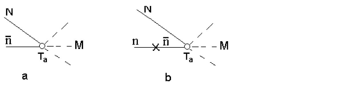
Figure 1: (a) Free-space $\bar{n}N$ annihilation. (b) Free-space process $n+N\rightarrow\bar{n}+N\rightarrow M$.

The matrix element of $S$-matrix $T_{a}$ and amplitude $M_{a}$ corresponding to Fig. 1a are defined as

$$iT_{a}=<\!M\!\mid T\exp(-i\int dx{\cal H}_{\bar{n}N}(x))-1\mid\!\bar{n}N\!>=N_{a}(2\pi)^{4}\delta^{4}(p_{f}-p_{i})M_{a}.$$ (12)

Here $<\!M\!\mid$ represents the annihilation mesons, ${\cal H}_{\bar{n}N}$ is the Hamiltonian of $\bar{n}N$ interaction, $N_{a}$ includes the normalization factors of the wave functions.

$T_{a}$ and $M_{a}$ involve all the $\bar{n}N$ interactions followed by annihilation including the $\bar{n}N$ rescattering in the initial state. The same is true for the subprocess of $\bar{n}N$ annihilation involved in Fig. 1b: the block $T_{a}$ should contain all the $\bar{n}N$ interactions followed by annihilation.

We write the formulas corresponding to Fig. 1b. The interaction Hamiltonian is

$${\cal H}_{I}={\cal H}_{n\bar{n}}+{\cal H}_{\bar{n}N}.$$ (13)

Formally, in the lowest order in ${\cal H}_{n\bar{n}}$ the amplitude of process (11) is given by

$$M_{1b}=\epsilon G_{0}M_{a},$$

$$G_{0}=\frac{1}{\epsilon_{n}-{\bf p}_{n}^{2}/2m}.$$ (14)

Here $G_{0}$ is the antineutron propagator. Since $M_{a}$ contains all the $\bar{n}N$ interactions followed by annihilation, $G_{0}$ is bare. We emphasize this fact as it gives an insight into origin of $\Sigma$.

Due to the zero momentum transfer in the $n\bar{n}$-transition vertex the 4-momenta of $n$ and $\bar{n}$ are equal. The both pre- and post-$n\bar{n}$ conversion spatial wave functions of the system coincide: $\mid\!Nn_{p}\!>_{{\rm sp}}=\mid\!N\bar{n}_{p}\!>_{{\rm sp}}$. Actually this is true for any neutron state (for any nuclear model).

For the time being we do not go into singularity $G_{0}\sim 1/0$. It results from the zero momentum transfer in the vertex corresponding to ${\cal H}_{n\bar{n}}$. The value of $\Sigma$ is disconnected with ${\cal H}_{n\bar{n}}$ and we want to separate these problems. The general consideration is given in Sect. 6.

4 $n\bar{n}$ transitions in the medium

In this section the origin of $\Sigma$ (energy gap) is studied in the framework of microscopic theory. It is shown that the value of $\Sigma$ is uniquely determined by the definition of the annihilation amplitude of $\bar{n}$ in the medium. It turns out that for a realistic definition $\Sigma=0$. Also we consider the competition between scattering and annihilation of $\bar{n}$ in the intermediate state.

4.1 $S$-matrix approach

Let us consider the process (2). (The $n\bar{n}$ transitions with $\bar{n}$ in the final state are considered in the next section.) We use the scheme identical to that for process (11) with the substitution $\bar{n}N\rightarrow(\bar{n}-\mbox{medium})$. The background field $U_{n}$ is included in the neutron wave function (Hamiltonian $H_{0}$); the quadratic terms ${\cal H}_{n\bar{n}}$ are included in the ${\cal H}_{I}$:

$${\cal H}_{I}={\cal H}_{n\bar{n}}+{\cal H},$$

$$H(t)=\int d^{3}x{\cal H}(x).$$ (15)

Here $H$ is the hermitian Hamiltonian of $\bar{n}$-medium interaction. The sole physical distinction with the model (4) is in the Hamiltonian ${\cal H}$. Recall that the potential model does not describe the processes (2) and (11) [5,6].

The process amplitude $M_{2}$ is uniquely determined by the Hamiltonian (15)

$$M_{2}=\epsilon G_{0}^{m}M_{a}^{m},$$

$$G_{0}^{m}=\frac{1}{\epsilon_{n}-{\bf p}_{n}^{2}/2m-U_{n}}$$ (16)

(see Fig. 2a). The matrix element of $S$-matrix $T_{fi}^{\bar{n}}$ and amplitude of antineutron annihilation in the medium $M_{a}^{m}$ are

$$iT_{fi}^{\bar{n}}=<\!f\!\mid T^{\bar{n}}\mid\!0\bar{n}_{p}\!>=N(2\pi)^{4}\delta^{4}(p_{f}-p_{i})M_{a}^{m},$$

$$T^{\bar{n}}=T\exp(-i\int_{-\infty}^{\infty}dtH(t))-1$$ (17)

(compare with Eq. (12)). Here $\mid\!0\bar{n}_{p}\!>$ is the state of the medium containing the $\bar{n}$ with the 4-momentum $p$, $<\!f\!\mid$ denotes the annihilation products, $N$ includes the normalization factors.

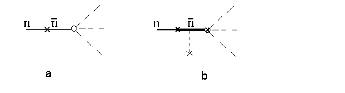
Figure 2: (a) $n\bar{n}$ transition in the medium followed by annihilation. The antineutron annihilation is shown by a circle. (b) Same as (a) but the antineutron propagator is dressed (see text).

The definition of the annihilation amplitude $M_{a}^{m}$ through Eqs. (17) is natural. If the number of particles of medium is equal to unity, Eq. (17) goes into (12). The annihilation width $\Gamma$ is expressed through $M_{a}^{m}$: $\Gamma\sim\int d\Phi\mid\!M_{a}^{m}\!\mid^{2}$. Since $H$ appears only in the $M_{a}^{m}$, the antineutron propagator $G_{0}^{m}$ is bare. In the next section we perform the rigorous calculation of $M_{2}$.

It is important that $M_{2}\sim M_{a}^{m}$. The value of $\Gamma$ and corrections to $M_{a}^{m}$ (if they are possible) have little effect on the results.

Construct now the model with the dressed propagator (see Fig. 2b). In the Hamiltonian ${\cal H}$ we separate out the real potential $V={\rm Re}U_{\bar{n}}-U_{n}$:

$${\cal H}=V\bar{\Psi}_{\bar{n}}\Psi_{\bar{n}}+{\cal H}^{\prime}$$ (18)

and include it in the antineutron Green function

$$G^{m}=G_{0}^{m}+G_{0}^{m}VG_{0}^{m}+...=\frac{1}{(1/G_{0}^{m})-V}=-\frac{1}{V}.$$ (19)

Then

$$M_{2}=\epsilon G^{m}M^{\prime}_{a},$$ (20)

$$G^{m}M^{\prime}_{a}=G_{0}^{m}M_{a}^{m}.$$ (21)

The propagator $G^{m}$ is dressed: $\Sigma=V\neq 0$. According to (21), the expressions for the propagator and vertex function are uniquely connected (if $H_{I}$ is fixed). The ”amplitude” $M^{\prime}_{a}(V,H^{\prime})$ should describe the annihilation. However, below is shown $M^{\prime}_{a}$ and model (20) are unphysical.

We recall the amplitude $M_{a}$ involves all the $\bar{n}N$ interactions followed by annihilation including rescattering in the initial state. Similarly, $M_{a}^{m}$ involves all the $\bar{n}$-medium interactions followed by annihilation including the antineutron rescattering in the initial state. Compare now the left- and right-hand sides of (21).

From the physical point of view model (20) has no justification on the following reasons.

1) If the number of particles of medium $n$ is equal to unity, the model (20) does not describe the free-space process (11) because Eq. (14) contains the bare propagator.

2) The observable values ($\Gamma$ for example) are expressed through $M_{a}^{m}$ and not $M^{\prime}_{a}$. Compared to $M_{a}^{m}$, $M^{\prime}_{a}$ is truncated because the portion of the Hamiltonian $H$ is included in $G^{m}$. $M^{\prime}_{a}$ has not a physical meaning.

(The formal expression for the dressed propagator should contain the annihilation loops as well. In this case the statements given in pp. 1) and 2) are only enhanced.)

3) Equations (19) and (20) mean that the annihilation is turned on upon forming of the self-energy part $\Sigma=V$ (after multiple rescattering of $\bar{n}$). This is counter-intuitive since at the low energies [15-17]

$$r=\frac{\sigma_{{\rm ann}}^{\bar{n}p}}{\sigma_{{\rm el}}^{\bar{n}p}}>2.5$$ (22)

and inverse picture takes place: in the first act of $\bar{n}$-medium interaction the annihilation occurs.

The realistic competition between scattering and annihilation should be taken into account. Both scattering and annihilation vertices should occur on equal terms in $M_{a}^{m}$ or $G^{m}$. According to pp. 1) and 2) the latest possibility should be excluded. In line with the physical meaning of $M_{a}^{m}$ and $M_{2}$, the amplitude (16) allows for the above-mentioned effect (see Sect. 4.3).

The structure with dressed propagator like (20) arises naturally if $V$ and ${\cal H}^{\prime}$ are the principally different terms and vertex function does not depend on $V$. In the problem under consideration this is not the case. This is evident from the formal expansion of the $T$-operator

$$T\exp(-i\int dx(V\bar{\Psi}_{\bar{n}}\Psi_{\bar{n}}+{\cal H}^{\prime})).$$ (23)

It is significant that even the non-realistic model (20) gives reinforcement in comparison with the potential model [5]:

$$\frac{W_{a}}{W_{t}^{{\rm pot}}}=1+\left(\frac{\Gamma/2}{V}\right)^{2}>1$$ (24)

because for the model (20) the probability of process (2) is

$$W_{a}\sim\Gamma$$ (25)

instead of $W_{t}^{pot}\sim 1/\Gamma$.

To summarize, the introducing of dressed propagator $G^{m}$ (energy gap) into process model entails an uncertainty of the vertex function $M^{\prime}_{a}$. The all-important effect of the competition is not taken into account. The limiting case $n=1$ is not reproduced. $M^{\prime}_{a}$ is unknown and unphysical.

We do not see the reasons for existence of field $V$ which should be included into $G^{m}$ and thus the antineutron propagator is bare. For the process sown in Fig. 8b the propagator is bare as well. Essentially, this fact is governing. Below we assume the definition (17) and consequently the model with the bare propagator (16).

4.2 Simplest model

The fact that the antineutron propagator is bare is obvious in the model containing the annihilation vertex only. We consider Fig. 1a. Assume that

$${\cal H}_{\bar{n}N}=\Phi^{*}_{M}g_{a}\Psi_{\bar{n}}\Psi_{N},$$ (26)

where $\Phi_{M}$ denotes the fields of mesons. The diagrams of the $\bar{n}N$ annihilation are shown in Fig. 3.

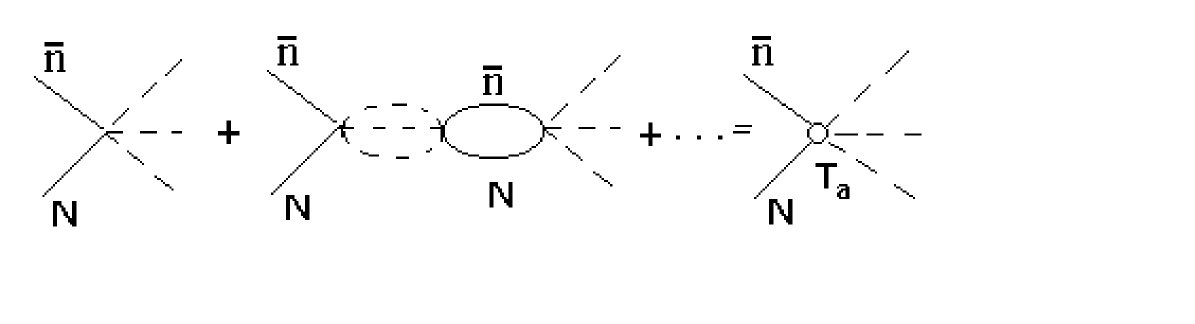
Figure 3: $\bar{n}N$ annihilation. The interaction Hamiltonian is given by Eq. (26).

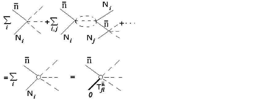
Figure 4: Antineutron annihilation in the medium.

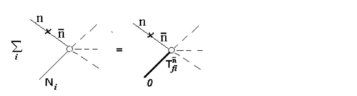
Figure 5: $n\bar{n}$ transition in the medium followed by annihilation.

Similarly, for the $\bar{n}$-medium annihilation we take

$${\cal H}={\cal H}_{a}=\sum_{i}\Phi^{*}_{M}g_{a}\Psi_{\bar{n}}\Psi_{N_{i}}.$$ (27)

The corresponding diagrams are shown in Fig. 4.

Consider now the process (2) using the same Hamiltonian ${\cal H}_{a}$. The diagram is shown in Fig. 5; the Hamiltonian is given by Eqs. (15), where ${\cal H}={\cal H}_{a}$. The antineutron propagator is bare. The questions connected with the self-energy part do not arise in principle because ${\cal H}_{a}$ must appear only in the $T_{fi}^{\bar{n}}$ (see Fig. 4). The block $T_{fi}^{\bar{n}}$ is described by Eqs. (17) and (27).

In view of Eq. (22), the models like (27) are reasonable and so it seems obvious that the antineutron propagator is bare.

4.3 Scattering and annihilation of $\bar{n}$ in the intermediate state

In the low-density limit the relative annihilation probability of the intermediate antineutron $r_{1}$ is [15-17]

$$r_{1}=\frac{\sigma_{a}}{\sigma_{t}}>0.7,$$ (28)

$\sigma_{t}=\sigma_{a}+\sigma_{s}$, where $\sigma_{a}$ and $\sigma_{s}$ are the cross sections of free-space $\bar{n}N$ annihilation and $\bar{n}N$ scattering, respectively. The ratio (28) or (22) is very important for the correct model construction.

The model given above reproduces the magnitudes of $r$ and $r_{1}$. Indeed, let us consider the free-space process

$$n+N\rightarrow\bar{n}+N\rightarrow f,$$ (29)

where $f$ denotes $\bar{n}N$ or $M$. The annihilation and scattering channels are defined by (11) and

$$n+N\rightarrow\bar{n}+N\rightarrow\bar{n}+N,$$ (30)

respectively. The corresponding diagrams are shown in Figs. 1b and 6a. Using the amplitude (14), the cross section of process (11) is found to be

$$\sigma^{nN}_{a}=N\int d\Phi\mid\!M_{1b}\!\mid^{2}=a^{2}N\int d\Phi\mid\!M_{a}\!\mid^{2}=a^{2}\sigma_{a},$$ (31)

$a=\epsilon G_{0}$. The normalization multiplier $N$ is the same for $\sigma^{nN}_{a}$ and $\sigma_{a}$.

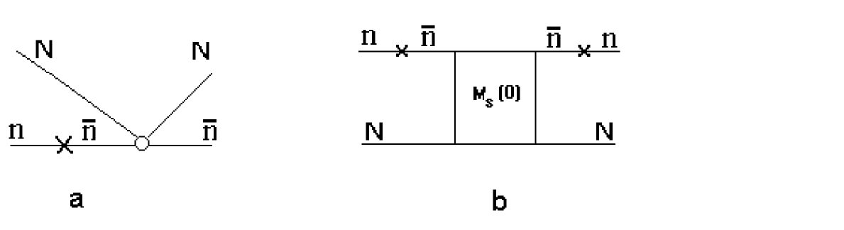
Figure 6: Free-space processes $n+N\rightarrow\bar{n}+N\rightarrow\bar{n}+N$ (Fig. a) and $n+N\rightarrow\bar{n}+N\rightarrow n+N$ (Fig. b).

For process (30) the similar calculation gives

$$\sigma^{nN}_{s}=a^{2}\sigma_{s}$$ (32)

and correspondingly

$$\frac{\sigma_{a}^{nN}}{\sigma_{s}^{nN}}=\frac{\sigma_{a}}{\sigma_{s}}=r.$$ (33)

The model (13) reproduces the ratio $r$.

For $n\bar{n}$ transition in the medium $r_{1}$ will be calculated by means of optical theorem. To check this calculation we obtain $r_{1}$ for free-space process (29) by means of optical theorem as well. The on-diagonal matrix element (see Fig. 6b) is

$$M(0)=\epsilon G_{0}M_{s}(0)G_{0}\epsilon=a^{2}M_{s}(0),$$ (34)

where $M_{s}(0)$ is the zero angle $\bar{n}N$ scattering amplitude. Let $\sigma^{nN}_{t}$ be the total cross section of process (29). Using the optical theorem in the left- and right-hand sides of (34), we get

$$\sigma^{nN}_{t}=a^{2}\sigma_{t}$$ (35)

and

$$\frac{\sigma_{a}^{nN}}{\sigma_{t}^{nN}}=\frac{\sigma_{a}}{\sigma_{t}}=r_{1}.$$ (36)

For process (29) the relative probability of the annihilation channel is given by (28), as we wished prove.

In the medium instead of (11) and (29) one should consider the process (2) and inclusive $n\bar{n}$ transition

$$(n-\mbox{medium})\rightarrow(\bar{n}-\mbox{medium})\rightarrow f_{m},$$ (37)

respectively. Here $f_{m}$ denotes $M$ or $\bar{n}$. The result is the same (see Appendix A): for process (37) the relative annihilation probability of the intermediate $\bar{n}$ is given by (28).

Ratio (28) is explicitly used only in the classical models like cascade one [18]. However, the Hamiltonian should contain all the needed information, which allows the calculation of $r$ or $r_{1}$. The fact that the model reproduces these ratios is very important; otherwise one can get a wrong, additional suppression as in model (20). Since the potential model does not describe the processes (11) and (2), it cannot reproduce (33) and (79).

The principal results of Sect. 4 are as follows. (a) The antineutron propagator is bare and singular. (b) In the low-density limit the ratio (28) should be reproduced. This can be considered as a necessary condition for the correct model construction. Model (15) satisfies this requirement.

5 Field-theoretical approach with finite time interval

The model must satisfy the following requirements: a) The $S$-matrix should be unitary. b) The model should reproduce the free-space process shown in Fig. 1 and competition between scattering and annihilation considered above. These conditions are obvious, however they are not fulfilled in the potential model.

The interaction Hamiltonian is given by Eq. (15). We use the basis $(n,\bar{n})$. The results do not depend on the basis. A main part of existing calculations have been done in $n-\bar{n}$ representation. The physics of the problem is in the Hamiltonian. The transition to the basis of stationary states is a formal step. It is possible only in the case of the potential model $H=V=$const., when the Hamiltonian of $\bar{n}$-medium interaction is replaced by the effective mass $H\rightarrow m_{{\rm eff}}={\rm Re}V-i\Gamma/2$. Since the calculation of process (2) will be done beyond the potential model, the procedure of diagonalization of mass matrix is unrelated to our problem.

The $S$-matrix amplitudes corresponding to Figs. 1b and 2a are singular as $G_{0}\sim 1/0$ and $G_{0}^{m}\sim 1/0$. Contrary to quantum electrodynamics, the formal sum of series in $\epsilon$ gives the meaningless self-energy $\Sigma\sim\epsilon^{2}/0$. This is because the Hamiltonian ${\cal H}_{n\bar{n}}$ corresponds to 2-tail. There is no compensation mechanism by radiative corrections.

For solving the problem the FTA is used [14]. It is infrared free. The calculation is performed by means of the evolution operator $U(t,0)$. The limiting transition $t\rightarrow\infty$ is not made as it is physically incorrect. The FTA can be used for any problem since for the nonsingular diagrams it converts to the $S$-matrix approach (see Sect. 6.1).

5.1 $n\bar{n}$ transitions with $\bar{n}$ in the final state

First of all we consider the $n\bar{n}$ transitions with $\bar{n}$ in the final states on the finite time interval $(t,0)$ (see Fig. 7).

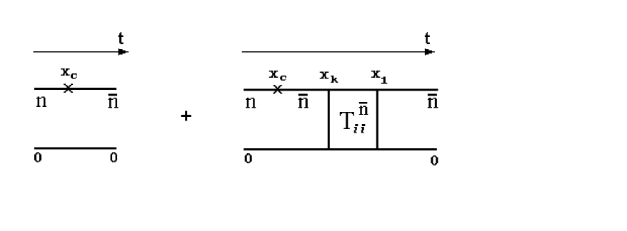
Figure 7: $n\bar{n}$ transition in the medium with $\bar{n}$ in the final state.

We introduce the evolution operator $U(t,0)=I+iT(t,0)$. In the lowest order in $\epsilon$ the matrix element $T_{\bar{n}n}$ is given by

$$<\!\bar{n}0\!\mid U(t,0)-I\mid\!0n\!>=iT_{\bar{n}n}(t,0)=-i<\!\bar{n}_{p}0\!\mid\int_{0}^{t}dt_{c}H_{n\bar{n}}(t_{c})+T^{\bar{n}}(t,0)\int_{0}^{t_{k}}dt_{c}H_{n\bar{n}}(t_{c})\mid\!0n_{p}\!>,$$ (38)

$$T^{\bar{n}}(t,t_{c})=T\exp(-i\int_{t_{c}}^{t}dt_{1}H(t_{1}))-1=\sum_{k=1}^{\infty}(-i)^{k}\int_{t_{c}}^{t}dt_{1}...\int_{t_{c}}^{t_{k-1}}dt_{k}H(t_{1})...H(t_{k}),$$ (39)

where $\mid\!0n_{p}\!>$ and $\mid\!0\bar{n}_{p}\!>$ are the states of the medium containing the neutron and antineutron with the 4-momentum $p=(\epsilon_{n},{\bf p}_{n})$, respectively; $T^{\bar{n}}$ is the $T$-operator of $\bar{n}$-medium interaction (compare with (17)).

We expand the $\Psi$-operators in the eigenfunctions of unperturbed Hamiltonian $H_{0}=-\nabla^{2}/2m+U_{n}$. Taking into account that $H_{n\bar{n}}\mid\!0n_{p}\!>=\epsilon\mid\!0\bar{n}_{p}\!>$, we change the order of integration [14] and obtain

$$T_{\bar{n}n}(t,0)=-\epsilon t-\epsilon\int_{0}^{t}dt_{c}iT^{\bar{n}}_{ii}(t-t_{c}),$$ (40)

$$iT^{\bar{n}}_{ii}(\tau)=<\!\bar{n}_{p}0\!\mid T^{\bar{n}}(\tau)\mid\!0\bar{n}_{p}\!>,$$

where $\tau=t-t_{c}$, $T^{\bar{n}}(\tau)=T^{\bar{n}}(t,t_{c})$. The $\bar{n}$-medium interaction is separated out in the block $T^{\bar{n}}_{ii}(\tau)$. This equation is important since the structure of matrix element corresponding to the process (2) is similar (see (64)). On the other hand, Eq. (40) can be verified with the use of the exactly solvable potential model.

5.2 Verification of FTA

To verify the FTA we obtain the results (5) and (6) of the potential model. As in Sect. 2, we take $H=V=$const. The block $T^{\bar{n}}_{ii}(\tau)$ is easily evaluated, resulting in

$$iT^{\bar{n}}_{ii}(\tau)=U^{\bar{n}}_{ii}(\tau)-1=\exp(-iV\tau)-1.$$ (41)

The probability of finding an $\bar{n}$ is

$$W_{\bar{n}}(t,0)=\mid\!T_{\bar{n}n}(t,0)\!\mid^{2}.$$ (42)

By means of Eqs. (40) and (41) it is easy to verify that $\mid\!T_{\bar{n}n}(t,0)\!\mid^{2}$ coincides with Eq. (5).

The total $n\bar{n}$ transition probability $W_{t}$ is given by

$$W_{t}(t,0)=1-\mid\!U_{ii}(t,0)\!\mid^{2}\approx 2{\rm Im}T_{ii}(t,0),$$ (43)

where $U_{ii}(t,0)=<\!n_{p}0\!\mid U(t,0)\mid\!0n_{p}\!>$. In the framework of the FTA the on-diagonal matrix element $T_{ii}$ has been calculated in Ref. [14]:

$$T_{ii}(t,0)=i\epsilon^{2}t^{2}/2-\epsilon^{2}\int_{0}^{t}dt_{\alpha}\int_{0}^{t_{\alpha}}dt_{c}T^{\bar{n}}_{ii}(t_{\alpha}-t_{c}).$$ (44)

Using Eqs. (41) and (44), one obtains that $2{\rm Im}T_{ii}=W_{t}^{{\rm pot}}$.

Consequently, the FTA reproduces all the results of the potential model. This was to be expected since one and the same Hamiltonian was used. The same is also true for any $ab$ transitions: $n\bar{n}$, $K^{0}\bar{K}^{0}$, neutrino oscillations. (The generalization for the relativistic case is trivial.)

5.3 Cancellation of divergences in the potential model

The consideration given above is infrared free. Let us return to the $S$-matrix problem formulation $(\infty,-\infty)$. Due to the zero momentum transfer in the $\epsilon$-vertex, any matrix element contains the singular propagator (see Figs. 7 and 8a). However, the matrix element of potential model $T_{ii}$ obtained by means of $S$-matrix approach is not singular (see Eq. (9)). The same is true for the process shown in Fig. 7. From microscopic theory standpoint the reason is as follows.

In addition to the singular propagator the matrix elements mentioned above also contain the block $T^{\bar{n}}_{ii}$ which is a sum of the zero angle rescattering diagrams of $\bar{n}$. As a result, the self-energy part $\Sigma=V$ appears. The corresponding mechanism of the cancellation of divergences (the forming of the self-energy part) is illustrated by Eq. (19), where $G_{0}^{m}\sim 1/0$.

We are interesting in off-diagonal matrix elements which do not contain the sum mentioned above ($T^{\bar{n}}_{f\neq i}$ instead of $T^{\bar{n}}_{ii}$) and hence diverges because one singular propagator after $\epsilon$-vertex appears in any case. (Recall that the formal sum of series in $\epsilon$ gives the meaningless self-energy part $\Sigma\sim\epsilon^{2}/0$.)

The principal result of this section is that the FTA has been verified by the example of the exactly solvable potential model. It is involved in the block $iT^{\bar{n}}_{ii}(\tau)=<\!\bar{n}_{p}0\!\mid T^{\bar{n}}(\tau)\mid\!0\bar{n}_{p}\!>$ as a special case.

6 $n\bar{n}$ transitions followed by annihilation

As shown above, the FTA reproduces all the potential model results. Besides, for non-singular diagrams it converts to the $S$-matrix theory (see Sect. 6.1). We now proceed to the main calculation.

Let us consider the process (2) in nuclear matter (see Fig. 8a). The Hamiltonians $H_{0}$ and $H_{I}(t)$ are the same as in Sect. 4. The 4-momenta of $n$ and $\bar{n}$ coincide. The $T^{\bar{n}}$-operator involves all the $\bar{n}$-medium interactions. In consequence of this $\Sigma=0$. In essence, we deal with 2-step nuclear decay: dynamical $n\bar{n}$ conversion, annihilation. Its dynamical part last only $10^{-24}$ s. The sole distinction with respect to the decay theory is that the FTA should be used because the antineutron propagator is singular.

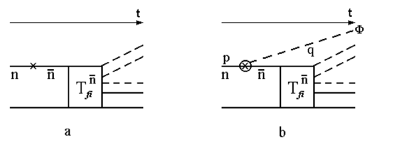
Figure 8: (a) $n\bar{n}$ transition in the medium followed by annihilation. (b) Same as (a) but with escaping of particle in the $n\bar{n}$ transition vertex.

We give the expressions for the amplitudes from Ref. [13]. Thereupon they will be obtained as a special case of a more general problem. The matrix element of the process shown in Fig. 8a is

$$T_{fi}(t)=-\epsilon\int_{0}^{t}dt_{c}iT^{\bar{n}}_{fi}(t,t_{c}),$$ (45)

$$iT^{\bar{n}}_{fi}(t,t_{c})=iT^{\bar{n}}_{fi}(\tau)=<\!f\!\mid T^{\bar{n}}(\tau)\mid\!0\bar{n}_{p}\!>.$$ (46)

Here $T^{\bar{n}}_{fi}(\tau)$ is the matrix element of the antineutron annihilation in a time $\tau=t-t_{c}$ (compare with the matrix element of $S$-matrix (17)). The $T^{\bar{n}}(\tau)$-operator is given by (39). Similarly to (40), the $\bar{n}$-medium annihilation is separated out in the block $T^{\bar{n}}_{fi}(\tau)$.

Consider now the more general problem. We calculate the matrix element $T_{fi}(t)$ shown in Fig. 8b on the interval $(t/2,-t/2)$. As a result, it will be shown that: (a) If $q\neq 0$ ($q$ is the 4-momentum of particle escaped in the $n\bar{n}$ transition vertex) and $t\rightarrow\infty$, we come to the usual $S$-matrix amplitude. (b) If $q\rightarrow 0$, Eq. (45) is obtained. Such scheme allows to verify and study the FTA. Also we will see the point in which the standard calculation scheme should be changed.

Consider the imaginary free-space decay

$$n\rightarrow\bar{n}+\Phi,$$ (47)

$\Phi(x)=N_{\Phi}\exp(-iqx),N_{\Phi}=(2q_{0}\Omega)^{-1/2}$. For decay to be permissible in vacuum put $m_{\bar{n}}=m-2m_{\Phi}$. As with ${\cal H}_{n\bar{n}}$, the decay Hamiltonian ${\cal H}^{\prime}_{n\bar{n}}$ is taken in the scalar form ${\cal H}^{\prime}_{n\bar{n}}=\epsilon^{\prime}\bar{\Psi}_{\bar{n}}\Phi^{*}\Psi_{n}+H.c.$.

The corresponding process in nuclear matter is shown in Fig. 8b. This is a nearest analogy to the process under study. The neutron wave function is $n_{p}(x)=N_{n}\exp(-ipx)$, where $N_{n}=\Omega^{-1/2}$, $p=(p_{0},{\bf p})$, $p_{0}=m+{\bf p}^{2}/2m$. The background nuclear matter field $U_{n}$ is omitted.

Instead of Eq. (15) we have

$$H_{I}=H^{\prime}_{n\bar{n}}+H,$$ (48)

$$H^{\prime}_{n\bar{n}}(t)=\epsilon^{\prime}\int d^{3}x(\bar{\Psi}_{\bar{n}}\Phi^{*}\Psi_{n}+H.c.);$$

$\epsilon^{\prime}$ is dimensionless. In the lowest order in $H^{\prime}_{n\bar{n}}$ the matrix element $T_{fi}(t)$ is

$$T_{fi}(t)=-<\Phi_{q}f0\mid\sum_{k=1}^{\infty}T_{k}(t)\int_{-t/2}^{t_{k}}dt_{c}H^{\prime}_{n\bar{n}}(t_{c})\mid\!0n_{p}\!>,$$

$$T_{k}(t)=(-i)^{k}\int_{-t/2}^{t/2}dt_{1}...\int_{-t/2}^{t_{k-1}}dt_{k}H(t_{1})...H(t_{k}).$$ (49)

Here $<\!f\!\mid$ represents the annihilation products with $(n)$ mesons. For the 3-tail ${\cal H}^{\prime}_{n\bar{n}}$ the relation $H_{n\bar{n}}\mid\!0n_{p}\!>=\epsilon\mid\!0\bar{n}_{p}\!>$ used in Sect. 5.1, is invalid. The direct calculation is needed.

Using the standard rules of quantum field theory, we obtain (see Appendix B)

$$T_{fi}(t)=-i\epsilon^{\prime}N_{n}N_{\Phi}<f0\mid\sum_{k=1}^{\infty}(-i)T_{k-1}(t)\int_{-t/2}^{t_{k-1}}dt_{k}\int d^{3}x_{k}{\cal H}^{\prime}(x_{k})e^{i({\bf p}-{\bf q}){\bf x}_{k}}I(t_{k})\mid 0\!>,$$ (50)

$$I(t_{k})=\int_{-\infty}^{\infty}\frac{dk_{0}}{2\pi}\int_{-t/2}^{t_{k}}dt_{c}\frac{1}{k_{0}-m_{\bar{n}}-({\bf p}-{\bf q})^{2}/2m_{\bar{n}}+i0}e^{-ik_{0}t_{k}}e^{it_{c}(q_{0}-p_{0}+k_{0})}.$$ (51)

From this point the calculations for Figs. 8a and 8b are essentially different. In Eq. (51) we put $t_{k}=\infty$ and $-t/2=-\infty$. Then

$$I(\infty)=\int\frac{dk_{0}}{2\pi}\frac{e^{-ik_{0}t_{k}}}{k_{0}-m_{\bar{n}}-({\bf p}-{\bf q})^{2}/2m_{\bar{n}}+i0}\int_{-\infty}^{\infty}dt_{c}e^{it_{c}(q_{0}-p_{0}+k_{0})}$$ (52)

and correspondingly

$$I(\infty)=Ge^{-i(p_{0}-q_{0})t_{k}},$$ (53)

$$G=\frac{1}{p_{0}-q_{0}-m_{\bar{n}}-({\bf p}-{\bf q})^{2}/2m_{\bar{n}}+i0},$$ (54)

where $G$ is the non-relativistic antineutron propagator.

Let $q=(0,0)$ and $m_{\bar{n}}=m$ (see Fig. 8a). Now

$$G=\frac{1}{p_{0}-m-{\bf p}^{2}/2m}\sim\frac{1}{0}$$ (55)

and $T_{fi}\sim 1/0$. This is an unremovable peculiarity. We deal with infrared divergence, what is obvious from Fig. 8a. We thus see the specific point (the limiting transition $t\rightarrow\infty$ in (50)) in which the standard $S$-matrix scheme should be changed.

6.1 Non-singular diagram

Obtain now the amplitudes corresponding to Figs. 8a and 8b starting from (50). If $q\neq 0$, the limit $t\rightarrow\infty$ can be considered. In Eq. (50) we put $t\rightarrow\infty$ and substitute Eq. (53). Taking into account that

$$N_{\bar{n}}e^{-i(p-q)x_{k}}\mid\!0>=\Psi_{\bar{n}}(x_{k})\mid\!\bar{n}_{p-q}\!>$$ (56)

and using the relation $\int d^{3}x_{k}{\cal H}^{\prime}(x_{k})\Psi_{\bar{n}}(x_{k})=H(t_{k})$ (see Appendix B), one obtains

$$T_{fi}=-iN_{\Phi}\epsilon^{\prime}G<f0\mid T^{\bar{n}}\mid\!0\bar{n}_{p-q}\!>.$$ (57)

Here $\mid\!0\bar{n}_{p-q}\!>$ is the state of the medium containing the $\bar{n}$ with the 4-momentum $p-q$, the $T^{\bar{n}}$-operator is given by (17). With the help of the relation

$$iT_{fi}=<\!f\!\mid T\mid\!i\!>=N(2\pi)^{4}\delta^{4}(p_{f}-p_{i})M_{fi}$$

we rewrite (57) in terms of the amplitudes

$$M_{8b}=\epsilon^{\prime}GM^{m}_{a}.$$ (58)

Here $M_{8b}$ is the amplitude of the process shown in Fig. 8b, $M^{m}_{a}$ is the annihilation amplitude of $\bar{n}$ with the 4-momentum $p-q$, $G$ is given by (54). We have obtained the usual $S$-matrix amplitude, which is the verification of (50). As in (16), the antineutron propagator is bare.

It is easy to estimate the widths corresponding to Fig. 8b and free-space decay (47):

$$\Gamma_{8b}\approx\epsilon^{\prime 2}\Gamma/(2\pi^{2}),$$

$$\Gamma_{{\rm free}}\approx\epsilon^{\prime 2}m_{\Phi}/(2\pi),$$ (59)

where we have put $m_{\Phi}/m\ll 1$. The $t$-dependence is determined by the exponential decay law

$$W_{8b,{\rm free}}=1-e^{-\Gamma_{8b,{\rm free}}t}\sim\Gamma_{8b,{\rm free}}t.$$ (60)

These formulas will be needed below.

6.2 Singular diagram

Let $q=0$ and $m_{\bar{n}}=m$ (see Fig. 8a). In (50) one should put $\epsilon^{\prime}=\epsilon$ and $N_{\Phi}=1$. Upon integration with respect to $k_{0}$, Eq. (51) becomes

$$I(t_{k})=-ie^{-it_{k}p_{0}}\int_{-t/2}^{t_{k}}dt_{c}.$$ (61)

As in (56), $N_{\bar{n}}\exp(-ipx_{k})\mid\!0>=\Psi_{\bar{n}}(x_{k})\mid\!\bar{n}_{p}\!>$. Turning back to the Hamiltonian $H(t_{k})$, one obtains

$$T_{fi}(t)=-i\epsilon<f0\mid\sum_{k=1}^{\infty}T_{k}(t)\int_{-t/2}^{t_{k}}dt_{c}\mid\!0\bar{n}_{p}\!>.$$ (62)

Using the formula

$$\int_{-t/2}^{t/2}dt_{1}...\int_{-t/2}^{t_{k-1}}dt_{k}\int_{-t/2}^{t_{k}}dt_{c}f(t_{1},...,t_{c})=\int_{-t/2}^{t/2}dt_{c}\int_{t_{c}}^{t/2}dt_{1}...\int_{t_{c}}^{t_{k-1}}dt_{k}f(t_{1},...,t_{c}),$$ (63)

we change the integration order and pass on to the interval $(t,0)$. Finally

$$T_{fi}(t)=-\epsilon\int_{0}^{t}dt_{c}<\!f0\!\mid T^{\bar{n}}(t-t_{c})\mid\!0\bar{n}_{p}\!>,$$ (64)

$$<\!f0\!\mid T^{\bar{n}}(\tau)\mid\!0\bar{n}_{p}\!>=iT^{\bar{n}}_{fi}(\tau),$$

which coincides with (45). The result is expressed through the submatrix $T^{\bar{n}}_{fi}(\tau)$. (Compare with (40).) Note that $T_{fi}(t)$ coincides with the second term of (40) with the replacement $<\!i\!\mid=<\!\bar{n}_{p}0\!\mid\rightarrow<\!f\!\mid$. This can be considered as a test for the $T_{fi}(t)$.

Comparing Eqs. (64) and (57), one can see the formal correspondence: if $q\rightarrow 0$, $GT_{fi}^{\bar{n}}\rightarrow i\int_{0}^{t}d\tau T^{\bar{n}}_{fi}(\tau)$.

7 Infrared singularities and the formulation of the S-matrix problem

In this section we consider the time-dependence of matrix elements and other characteristic features of the FTA and complete the calculation of process (2) (see also [13]).

The FTA is infrared-free. It naturally connected with the conditions of experiment. Indeed, measurement of any process corresponds to some interval $\tau$. So it is necessary to calculate $U_{fi}(\tau)$. The replacement $U(\tau)\rightarrow S(\infty)$ is justified if the main contribution gives some region $\Delta<\tau$, so that $U_{fi}(\tau>\Delta)=U_{fi}(\infty)=S_{fi}=$const. The expressions of this type are the basis for all $S$-matrix calculations. The following cases are possible.

1. There is bound to be asymptotic regime. Then the usual scheme realized in field theory or non-stationary theory of scattering takes place. Fig. 8b corresponds to this case.

2. There is no asymptotic regime. An example is provided by oscillation hamiltonian ${\cal H}_{n\bar{n}}$. We have usual non-stationary problem. The $S$-matrix approach is inapplicable. Because of this, for Fig. 8a the calculation has been done in the framework of FTA.

A somewhat different explanation of application of the FTA is as follows. If ${\cal H}_{I}={\cal H}_{n\bar{n}}$, the solution is periodic. It is obtained by means of non-stationary equations of motion and not $S$-matrix theory. This is clear from the $S$-matrix definition. To reproduce the limiting case ${\cal H}\rightarrow 0$, i.e. the periodic solution, we have to use the FTA.

Let us return to Eq. (64). The annihilation of $\bar{n}$ in nuclear matter can be considered as the decay of a one-particle state with the characteristic time $\tau_{a}$. Correspondingly, $T^{\bar{n}}_{fi}$ can be interpreted as the decay matrix of the $\bar{n}$-medium state. Obviously

$$T^{\bar{n}}_{fi}(\tau>\tau_{a})\approx T^{\bar{n}}_{fi}={\rm const.}$$ (65)

and

$$W^{\bar{n}}=\sum_{f\neq i}\mid T_{fi}^{\bar{n}}\mid^{2}=1,$$ (66)

where $W^{\bar{n}}$ is the total decay probability of the $\bar{n}$-nucleus. Let

$$t\gg\Delta\approx\tau_{a}.$$ (67)

In view of this condition the submatrix $T_{fi}^{\bar{n}}$ can be calculated by means of $S$-matrix theory. The FTA is needed only for description of the subprocess of the $n\bar{n}$ conversion. However, the condition (66) greatly simplifies the calculation. One can write immediately [13]

$$W_{a}(t)\approx\sum_{f\neq i}\mid-i\epsilon tT_{fi}^{\bar{n}}\mid^{2}=\epsilon^{2}t^{2}W^{\bar{n}}=\epsilon^{2}t^{2}=W_{f}(t),$$ (68)

where $W_{a}(t)$ is the probability of process (2).

For $n\bar{n}$ transitions in nuclear $W_{t}(t)=W_{a}(t)$ since all the $\bar{n}$ annihilate. The interpretation of $W_{a}(t)$ has been given above: momentary $n\bar{n}$ conversion at some point in time between $0$ and $t$; annihilation in a time $\tau_{a}\sim 6\times 10^{-24}$ s. The explanation of the $t^{2}$-dependence is simple. The process shown in Fig. 8a represents two consecutive subprocesses. The speed and probability of the whole process are defined by those of slower subprocess. Since $\tau_{a}\ll t$, the annihilation can be considered instantaneous: for any $t_{1}<t$ the annihilation probability is $W^{\bar{n}}(t-t_{1})\approx 1$. So, the probability of process (2) is defined by the speed of $n\bar{n}$ transition: $W_{a}\approx W_{f}\sim t^{2}$, but not $\sim t/\Gamma$ (see Eq. (6)). In essence, we deal with the limiting case $\tau/t\rightarrow 0$ or, similarly, $T^{\bar{n}}_{fi}(\tau)=T^{\bar{n}}_{fi}$ at any $\tau$. Formally, the quadratic time-dependence follows from (64).

Owing to annihilation channel, $W_{a}$ is practically equal to the free-space $n\bar{n}$ transition probability. So $\tau_{n\bar{n}}\sim T_{n\bar{n}}$, where $T_{n\bar{n}}$ is the oscillation time of neutron bound in a nucleus.

All the results have been obtained by means of formal expansions. They are valid at any finite $t$. Consequently, the singularities of the $S$-matrix amplitudes $M_{1b}$ and $M_{2}$ result from the erroneus problem formulation. The problem should be formulated on the finite interval $(t,0)$. If $t\rightarrow\infty$, Eq. (68) diverges just as the modulus (16) squared does. The infrared singularities point to the fact that there is no asymptotic regime.

8 Summary and discussion

The importance of unitarity condition is well known [19-21]. Nevertheless, the non-hermitian models are frequently used because on the one hand, they greatly simplify the calculation and on the other hand, it is hoped that an error may be inessential. This paper demonstrates that the non-unitarity of $S$-matrix can produce a qualitative error in the results. Certainly, the unitarity is a necessary and not sufficient condition. We compare our results and potential model one.

The time-dependence is a more important characteristic of any process. It is common knowledge that $t$-dependence of decay probability in the vacuum and medium is identical. Equations (60) illustrate this fact. In our calculation the $t$-dependencies coincide as well: $W_{a}\sim W_{t}\sim t^{2}$ and $W_{f}\sim t^{2}$. The potential model gives $W_{t}^{{\rm pot}}\sim t$, whereas $W_{f}\sim t^{2}$. It is beyond reason to such fundamental change.

The $\Gamma$-dependence of the results differs fundamentally as well. The probability of the decay shown in Fig. 8b is linear in $\Gamma$

$$W_{8b}=\Gamma_{8b}t\sim\Gamma t$$ (69)

(see (59) and (60)). For Fig. 8a the annihilation effect acts in the same direction

$$W_{a}\sim W^{\bar{n}}\sim\Gamma.$$ (70)

In the potential model the effect of absorption acts in the opposite direction $W_{t}^{{\rm pot}}\sim 1/\Gamma$. Recall that the annihilation is the basic effect determining the process speed (see (6) and (68)).

Let us consider the suppression factor $R$. From Eq. (68) we have

$$R=\frac{W_{a}}{W_{f}}\sim 1.$$ (71)

For similar processes the value $R\sim 1$ is typical. Indeed, in the medium the free-space decay (47) suppressed by the factor

$$\frac{\Gamma_{8b}}{\Gamma_{{\rm free}}}=\frac{\Gamma}{\pi m_{\Phi}}\approx\frac{1}{\pi},$$ (72)

where we have put $m_{\Phi}\approx\Gamma$.

The realistic example is the pion production $pn\rightarrow pp\pi^{-}$ in vacuum and on neutron bound in a nucleus. If the pion energy is in the region of resonance, the pion absorption is very strong. This effects on the number of pions emitted from the nucleus, but not on the fact of pion formation inside the nucleus. (In the latter case the pion and products of pion absorption should be detected).

In the processes cited above $R\sim 1$. The potential model gives $R_{{\rm pot}}\rightarrow 0$: if $\Gamma\sim 100$ MeV and $t\sim 1$ yr [22], $R_{{\rm pot}}\sim 10^{-30}$.

Consequently, in the potential model the $t$- and $\Gamma$-dependencies are principally incorrect. As a result, the suppression is enormous: $R_{{\rm pot}}\rightarrow 0$. This is not surprising since the potential model describes only $W_{\bar{n}}$. Recall that in the strong absorption region $W_{\bar{n}}\ll W_{a}$.

The next important point is the competition between scattering and annihilation in the intermediate state. The models (13) and (15) reproduce the values of $r$ and $r_{1}$ (see Sect. 4.3). Since the potential model does not describe the processes (2) and (11), it makes no sense to speak about competition effect in this model. The greater the $|{\rm Im}V|$, the greater an error in the $W_{t}^{{\rm pot}}$ and $W_{a}$ calculated by means of potential model.

Consider now the effects of coherent forward scattering and absorption. Let there is a forward scattering alone: $H={\rm Re}V$. Since the FTA reproduces all the potential model results (see Sect. 5.2), it describes the above-mentioned special case as well, in particular, the suppression of oscillations by ${\rm Re}V$.

Let there is an annihilation vertex only: $V=0$ and

$${\cal H}={\cal H}_{a}.$$ (73)

The annihilation Hamiltonian ${\cal H}_{a}$ is given by (27). In this case we inevitably arrive at the amplitude with singular propagator. The dressed propagator cannot arise in principal (see Sect. 4.2). In view of Eq. (22) the model (73) is reasonable and so the result $W_{a}\approx W_{f}$ seems quite natural for us. In our calculation the approximation (73) has been not used. Nevertheless, the result is the same as in model (73). In this connection we briefly outline the principal points of our calculation.

The process shown in Fig. 8b is described by the Hamiltonian $H_{I}=H^{\prime}_{n\bar{n}}+H$. Since $H$ appears in the block $T^{\bar{n}}_{fi}$ only, the antineutron propagator is bare. For Fig. 8a the picture is the same, however $T_{fi}\sim 1/0$ (here we keep in mind the $S$-matrix problem formulation). Due to of this we had to use the FTA.

The fact that antineutron propagator is bare is principal. It entails the divergence of the $S$-matrix amplitude; the application of FTA; the linear time-dependence of the matrix element $T_{fi}(t)$ and $t^{2}$-dependence of the result. In our opinion the models with dressed (and consequently non-singular) propagator are non-realistic (see Sect. 4).

(Recall that in the potential model the antineutron propagator is dressed as $\Sigma=V$ by the model construction. Since this model is inapplicable, the field-theoretical approach is used. The self-energy should be considered in the context of the concrete problem. Obviously, for Fig. 8b the propagator is bare. For Fig. 8a it is bare as well because the $\bar{n}$-medium interaction is the same.)

All the formulas up to (64) are true for any $ab$ transitions in which $m_{a}=m_{b}$. (A generalizations for the relativistic case and the case when $m_{a}\neq m_{b}$ are simple.) The next important point is the condition (67). For $n\bar{n}$ transitions in nuclei it is obvious because in this case the value $t=T_{0}=1.3$ yr [22] is used ($T_{0}$ is the observation time in a proton-decay type experiment). The condition $t\gg\tau_{a}$ leads to Eqs. (65) and (66). Due to of them the result does not depend on a specific form of $H$ and coincides with the result given by the model (73).

Once the antineutron annihilation amplitude is defined by (46), the rest of calculation is rather formal. The distinguishing features of the model is that the process amplitude is ”propotional” to the annihilation amplitude $T_{fi}\sim T^{\bar{n}}_{fi}$. This structure is typical for the direct processes.

If the condition $t\gg\Delta$ is not fulfilled, the direct calculation of (64) is needed. However, the qualitative picture remains the same: the process amplitude is proportional to the absorption amplitude.

It is interesting to study the behavior of $W_{t}$ in the intermediate range $t\sim\Delta$. It seems plausible that $W_{t}$ depends slightly on the value of $\Delta/t$ (in comparison with potential model results). We also note that there is no asymptotic regime for free-space $K^{0}\bar{K}^{0}$ oscillations. In our opinion, it makes sense to look at the calculation of $\Delta m=m_{L}-m_{S}$ (GIM mechanism) from the standpoint of applicability of $S$-matrix approach in this case (see Sect. 7).

9 Conclusion

The approach considered above reproduces all the results on the particle oscillations (Sect. 5.2). Certainly, for the problems where the absorption is inessential, the standard model of oscillations is more handy since it is more simple. Our approach is oriented to the processes like (1) which are not described by the potential model.

The direct calculation of $n\bar{n}$ transitions in nuclear matter followed by annihilation has been done. The results have been discussed in Sect. (8). We confirm our restriction [13] on the free-space $n\bar{n}$ oscillation time $\tau_{n\bar{n}}>10^{16}$ yr. Compared to [13], the result (68) was obtained as a special case of a more general problem. Besides, the medium corrections, the uncertainties related to amplitudes and competition between scattering and annihilation in the intermediate state have been studied. The model (73) and analysis made in Sect. 4 show that $\Sigma=0$. Nevertheless, this is a point of great nicety. The further investigations are desirable. The region $t<\Delta$ and oscillations of another particles can be considered as well.

The calculation up to (64) is formal. With the replacement $T^{\bar{n}}_{fi}(\tau)\rightarrow T^{b}_{fi}(\tau)$, where $T^{b}_{fi}$ is the $b$-particle absorption amplitude, the matrix element (64) describes the process (1) in which $m_{a}=m_{b}$. In this connection we point out some features of Eq. (64). a) The amplitude $T_{fi}(t)$ is ”proportional” to the amplitude $T_{fi}^{b}(\tau)$. In the potential model the effect of $b$-particle absorption acts in the opposite direction, which tends to suppress the process. b) In the lowest order in $\epsilon$ the potential model gives the linear $t$-dependence $W_{t}^{{\rm pot}}\sim t/\Gamma$. For any block $T_{fi}^{b}(\tau)$ model the time-dependence of the value $\mid T_{fi}(t)\mid^{2}$ cannot be linear.

Also we would like to emphasize that for a processes with zero momentum transfer the problem should be formulated on the finite time interval.

Appendix A
In this appendix the relative annihilation probability of the intermediate $\bar{n}$ for $n\bar{n}$ transition in the medium is calculated. Similarly to (31), we obtain the probability of process (2) in a unit of time

$$\Gamma_{2}=N_{1}\int d\Phi\mid\!M_{2}\!\mid^{2}=a^{2}_{m}N_{1}\int d\Phi\mid\!M_{a}^{m}\!\mid^{2}=a^{2}_{m}\Gamma,$$ (74)

$a_{m}=\epsilon G_{0}^{m}$. The normalization multiplier $N_{1}$ is the same for $\Gamma_{2}$ and $\Gamma$. The term ”width” is unused because the $t$-dependence of process (2) does not need to be $\exp(-\Gamma_{2}t)$ (see Sect. 7).

In the low-density approximation [23,24] $\Gamma=v\rho\sigma_{a}$ and

$$\Gamma_{2}=a_{m}^{2}v\rho\sigma_{a}.$$ (75)

The on-diagonal matrix element $M^{m}(0)$ corresponding to the process $(n-\mbox{medium})\rightarrow(\bar{n}-\mbox{medium})\rightarrow(n-\mbox{medium})$ is

$$M^{m}(0)=\epsilon G_{0}^{m}M^{m}_{s}(0)G_{0}^{m}\epsilon=a^{2}_{m}M^{m}_{s}(0)$$ (76)

(compare with (34)). Here $M^{m}_{s}(0)$ is the amplitude of zero angle scattering of $\bar{n}$ in the medium.

Taking into account that

$$\frac{1}{T_{0}}2{\rm Im}M^{m}(0)=\Gamma_{t},$$ (77)

$$\frac{1}{T_{0}}2{\rm Im}M^{m}_{s}(0)=v\rho\sigma_{t}$$

($T_{0}$ is the normalization time, $\Gamma_{t}$ is the probability of the process (37) in a unit of time), one obtains

$$\Gamma_{t}=a_{m}^{2}v\rho\sigma_{t}$$ (78)

and correspondingly

$$\frac{\Gamma_{2}}{\Gamma_{t}}=r_{1}.$$ (79)

Equations (75) and (78) are interpreted in line with the low-density approximation physics.

Appendix B
The calculation is standard [25,26] up to the integration over $t$. The neutron and antineutron are assumed spinless. We have

$$\Psi_{n}(x)\mid\!n_{p}\!>=\Psi_{n}(x)b^{+}(p)\mid\!0\!>=N_{n}e^{-ipx}\mid\!0>,$$ (80)

$$<\Phi_{q}\mid\Phi^{*}(x)=<0\mid N_{\Phi}e^{iqx}.$$ (81)

Then

$$<\Phi_{q}\mid\Phi^{*}(x_{c})\Psi_{\bar{n}}(x_{c})\mid\!n_{p}\!>=N_{n}N_{\Phi}e^{i(q-p)x_{c}}.$$ (82)

In the last multiplier of Eq. (49) we separate out the antineutron field operator $\Psi_{\bar{n}}(x_{k})$:

$$H(t_{k})=\int d^{3}x_{k}{\cal H}(x_{k})=\int d^{3}x_{k}{\cal H}^{\prime}(x_{k})\Psi_{\bar{n}}(x_{k}).$$ (83)

Equation (49) becomes

$$T_{fi}(t)=-i\epsilon^{\prime}N_{n}N_{\Phi}<f0\mid\sum_{k=1}^{\infty}(-i)T_{k-1}(t)\int_{-t/2}^{t_{k-1}}dt_{k}\int d^{3}x_{k}{\cal H}^{\prime}(x_{k})J(t_{k})\mid\!0>,$$ (84)

$$J(t_{k})=\int_{-t/2}^{t_{k}}dt_{c}\int d^{3}x_{c}<T(\Psi_{\bar{n}}(x_{k})\bar{\Psi}_{\bar{n}}(x_{c}))>e^{i(q-p)x_{c}}.$$ (85)

For Fig. 8a the problem is non-relativistic and so for Fig. 8b we also take the non-relativistic antineutron propagator

$$<T(\Psi_{\bar{n}}(x_{k})\bar{\Psi}_{\bar{n}}(x_{c}))>=iG(x_{k}-x_{c})=i\int\frac{dk_{0}}{2\pi}e^{-ik_{0}(t_{k}-t_{c})}\int\frac{d^{3}k}{(2\pi)^{3}}\frac{e^{i{\bf k}({\bf x}_{k}-{\bf x}_{c})}}{k_{0}-m_{\bar{n}}-{\bf k}^{2}/2m_{\bar{n}}+i0}.$$ (86)

Upon integrating over ${\bf x}_{c}$ and ${\bf k}$ we obtain Eqs. (50) and (51).

References

- [1] M. L. Good, Phys. Rev. 106 (1957) 591 ; Phys. Rev. 110 (1958) 550.
- [2] L. Wolfenstein, Phys. Rev. D 17 (1978) 2369.
- [3] E. D. Commins and P. H. Bucksbaum, Weak Interactions of Leptons and Quarks (Cambridge University Press, 1983).
- [4] F. Boehm and P. Vogel, Physics of Massive Neutrinos (Cambridge University Press, 1987).
- [5] V. I. Nazaruk, Mod. Phys. Lett. A 21 (2006) 2189; V. I. Nazaruk, Proceedings of the 9th International Conference on Low Energy Antiproton Physics (LEAP’05), Bonn, Germany 2005, edited by D.Grzonka, R. Czyzykiewich, W.Oelert, T.Rozek, P.Winter, AIP Conf. Proc. 796 (2005) 180.
- [6] V. I. Nazaruk, Eur. Phys. J. A. 31 (2007), Online-first, e-print DOI 10.1140/epja/i2006-10164-y.
- [7] V. A. Kuzmin, JETF Lett. 12 (1970) 228.
- [8] S. L. Glashow, preprint HUTP-79/A059 (Harvard, 1979).
- [9] R. N. Mohapatra and R. E. Marshak, Phys. Rev. Lett. 44 (1980) 1316.
- [10] P. G. H. Sandars, J. Phys. G 6 (1980) L161.
- [11] M. V. Kazarnovsky et al., Pis’ma Zh. Eksp. Teor. Fiz. 32 (1980) 88; K. G. Chetyrkin et al., Phys. Lett. B 99 (1981) 358.
- [12] J. Arafune and O. Miyamura, Prog. Theor. Phys. 66 (1981) 661.
- [13] V. I. Nazaruk, Phys. Rev. C 58 (1998) R1884.
- [14] V. I. Nazaruk, Phys. Lett. B 337 (1994) 328.
- [15] T. Kalogeropouls and G. S. Tzanakos, Phys. Rev. D 22 (1980) 2585.
- [16] G. S. Mutchlev et al., Phys. Rev. D 38 (1988) 742.
- [17] W. Bruckner et al., preprint CERN-EP/89-105 (Geneve 1989).
- [18] A. S. Iljinov, V. I. Nazaruk and S. E. Chigrinov, Nucl. Phys. A 382 (1982) 378.
- [19] T. Inone and E. Oset, Nucl. Phys. A 710 (2002) 354.
- [20] T. Inone and E. Oset, Nucl. Phys. A 721 (2003) 661.
- [21] E. Oset, Nucl. Phys. A 721 (2003) 58.
- [22] H. Takita et al., Phys. Rev. D 34 (1986) 902.
- [23] C. B. Dover, J. Hufner and R. H. Lemmer, Ann. Phys. 66 (1971) 248.
- [24] J. Hufner, Phys. Rep. 21 (1975) 1.
- [25] J. D. Bjorken and S. D. Drell, Relativistic Quantum Fields (New York, Mc Graw-Hill, 1964).
- [26] T. Ericson and W. Weise, Pions and Nuclei (Clarendon Press, Oxford, 1988).