Absorption in the final state in reactions and decays in the medium

Abstract

The role of strong absorption of particles in intermidiate and final states has been considered. The range of applicability of phenomenological model of absorption has been studied. This model is nonuniversal. Its applicability depends on the type of interaction Hamiltonian and matrix element used. We also demonstrate that the violation of the unitarity condition can produce a qualitative error in the results. The absorption (decay) in the final state does not tend to suppress the total process probability as well as the probability of the channel corresponding to absorption. This is true for the reactions, decays and $n\bar{n}$ conversion in the medium.

PACS: 24.10.-i, 24.50.+g, 11.30.Fs

*E-mail: nazaruk@inr.ru

1 Introduction

In [1] it was shown that in field-theoretical and phenomenological models the effect of final state absorption acts in the opposite directions. In the following this problem is considered in detail. We adduce an additional arguments and study the reasons for this disagreement. This also makes sense if one considers that some problems were solved by means of the above-mentioned phenomenological models only. Also we study the range of applicability of phenomenological models.

Phenomenologically, the absorption is described by an optical potential [2]. For illustration, let us consider a free-space decay $a\rightarrow b\bar{n}$, for example, $\bar{\Lambda}\rightarrow\bar{n}\pi^{0}$. For a decay in nuclear matter we have

$$a\rightarrow b+\bar{n}\rightarrow b+M$$ (1)

($M$ are the annihilation mesons) because $\bar{n}$ annihilates in a time $\tau\sim 10^{-24}$ s.

By way of another example we consider the $n\bar{n}$ transitions [3-5] in nuclear matter followed by annihilation

$$n\rightarrow\bar{n}\rightarrow M.$$ (2)

The antineutron annihilation should be described by an Hermitian Hamiltonian ${\cal H}_{a}$. In the phenomenological models

$${\cal H}_{a}\rightarrow{\cal H}=i{\rm Im}U_{\bar{n}}\bar{\Psi}_{\bar{n}}\Psi_{\bar{n}},$$ (3)

where $U_{\bar{n}}$ is the optical potential of $\bar{n}$, ${\cal H}$ is the phenomenological absorption (annihilation) Hamiltonian. For brevity, ${\rm Re}U_{\bar{n}}$ will be omitted, except if otherwise noted.

In practice, the absorption and decay are described by a distorted wave [6], or dressed propagator (see, for example, refs. [7,8]). To study the model as a whole, one should write the total interaction Hamiltonian ${\cal H}_{I}$. In specific calculations the Hamiltonian ${\cal H}$, as a rule, is not adduced. However, the corresponding terms in the distorted wave or Green function originate from ${\cal H}$. Due to this, we consider the problem at the level of the effective (not fundamental) Hamiltonians.

In the case of process (1), the phenomenological model is given by

$${\cal H}_{I}={\cal H}_{1}+{\cal H}_{a}\rightarrow{\cal H}_{1}+{\cal H},$$ (4)

where ${\cal H}_{1}$ is the Hamiltonian of the free-space decay $a\rightarrow b\bar{n}$.

The phenomenological interaction Hamiltonian of process (2) is

$${\cal H}_{I}={\cal H}_{n\bar{n}}+{\cal H},$$

$${\cal H}_{n\bar{n}}=\epsilon\bar{\Psi}_{\bar{n}}\Psi_{n}+H.c.,$$ (5)

$\epsilon=1/\tau$. Here ${\cal H}_{n\bar{n}}$ is the Hamiltonian of $n\bar{n}$ conversion [5], $\tau$ is the free-space ${n\bar{n}}$ oscillation time. As we will see later, process (2) is an ideal instrument for the study of the final state absorption and we focus on this process.

On the one hand, model (3) is very useful because it greatly simplifies the calculation. On the other hand, the Hamiltonian ${\cal H}$ is non-hermitian and so model (3) is effective. Its applicability range is restricted.

We consider the decay $a\rightarrow b\bar{n}$ and the $n\bar{n}$ transition in the medium and elucidate what processes can be described by the effective Hamiltonians (4) and (5). More complicated processes are considered as well. In other words, we study the range of applicability of model (3). We also study the suppression of the processes mentioned above due to final state absorption. This is a question of principal because the calculations with hermitian and non-hermitian Hamiltonians give opposite results.

For our purposes it is sufficient to consider the simplest potential $U_{\bar{n}}=$const. We perform concrete calculations and show that the unjustified application of a model can produce a qualitative error in the results. This is primarily true for the total probability of decays, $n\bar{n}$ transitions and reactions. Formally, models (4) and (5) can lead to an additional suppression of the total process probability as well as of the probability of the channel corresponding to absorption in comparison with the calculations with hermitian ${\cal H}_{a}$ or, similarly, calculations with hermitian ${\cal H}_{a}$ can tend to increase the above-mentioned values.

With the substitution $i{\rm Im}U_{\bar{n}}=-i\Gamma_{x}/2$, where $\Gamma_{x}$ is the width of some free-space decay $\bar{n}\rightarrow x$, the effective Hamiltonians (4) and (5) describe the free-space two-step processes: $a\rightarrow b+\bar{n}\rightarrow b+x$ and $n\rightarrow\bar{n}\rightarrow x$, respectively. So, when referring to Hamiltonian ${\cal H}$, we keep in mind the decay as well.

The paper is organized as follows. In sect. 2 the simple but important statement related to the final state interaction is proven: the opening of a new channel leads to increase the total decay probability. It turns out, that for the $n\bar{n}$ conversion in the medium model (5) contradicts this statement (sect. 3). The same is also true for the free-space decay (sect. 4). Section 5 shows that the reason for this is the non-unitarity of the $S$-matrix and the structure of the Green function. In this connection we review the origin of the complex self-energy $\Sigma$ in quantum electrodynamics (QED) and optical potential theory and point out the principal distinctions with respect to the model under study (sects. 5 and 6). The value and physical meaning of $i{\rm Im}U$ for various ${\cal H}_{I}$ are analyzed as well. In sect. 7, we qualitatively discuss more complicated Hamiltonians and matrix elements. Field-theoretical and phenomenological approaches are compared in sect. 8. The results are summarized and discussed in sect. 9.

2 Absorption in the final state

To clarify the role of final state absorption, we prove a simple model-independent statement. We consider the decay $a\rightarrow b\bar{n}$ in the medium. Let ${\cal H}_{s}$ and ${\cal H}_{a}$ be the hermitian Hamiltonians of the scattering and annihilation of $\bar{n}$, respectively. The total $a$-particle decay probability $W_{t}$ is $W_{t}=W_{\bar{n}}+W_{a}$, where $W_{\bar{n}}$ and $W_{a}$ are the probabilities of finding an antineutron and annihilation mesons $M$, respectively (see fig. 1).

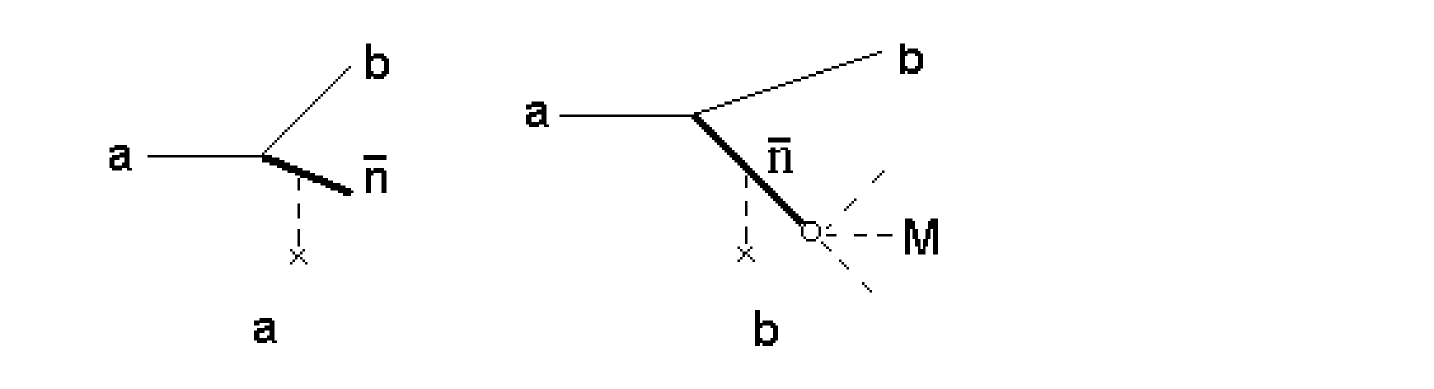
Figure 1: (a) The decay $a\rightarrow b+\bar{n}$ in the medium without considering annihilation. (b) The same as (a), but with annihilation. The antineutron annihilation is illustrated by a circle.

Let ${\cal H}_{a}=0$ and ${\cal H}_{s}\neq 0$, then $W_{t}=W_{\bar{n}}$ (see fig. 1a). Now, let us turn on the perturbation ${\cal H}_{a}$ (see fig. 1b). In the lowest order in ${\cal H}_{a}$ we have

$$W_{t}({\cal H}_{s}+{\cal H}_{a})=W_{\bar{n}}({\cal H}_{s}+{\cal H}_{a})+W_{a}({\cal H}_{s}+{\cal H}_{a})>W_{\bar{n}}({\cal H}_{s}+{\cal H}_{a})=W_{\bar{n}}({\cal H}_{s}+0)=W_{t}({\cal H}_{s}+0).$$

Thus,

$$W_{t}({\cal H}_{s}+{\cal H}_{a})>W_{t}({\cal H}_{s}+0).$$ (6)

In the equality $W_{\bar{n}}({\cal H}_{s}+{\cal H}_{a})=W_{\bar{n}}({\cal H}_{s}+0)$ it was taken into account that only terms of zero order in ${\cal H}_{a}$ give a contribution to $W_{\bar{n}}$. Inequality (6) can be written in terms of decay widths. We use the probabilities for reasons given in sect. 5.

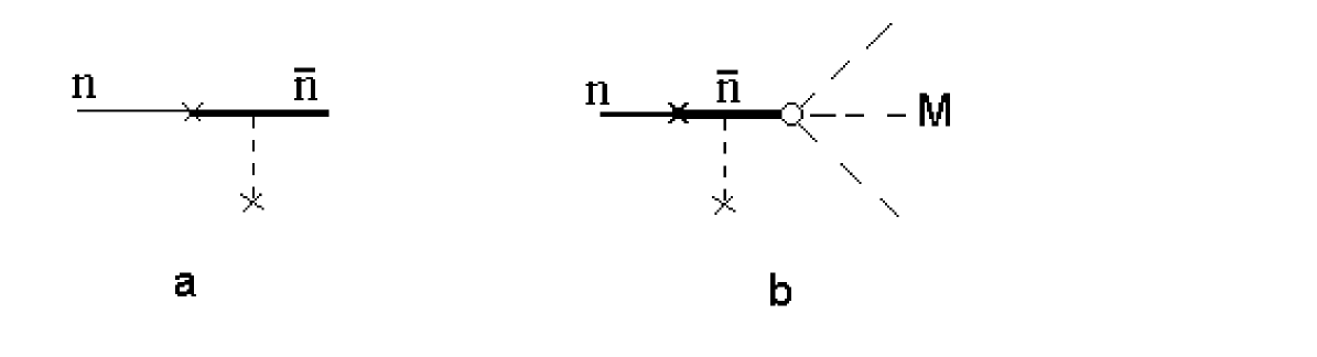
Figure 2: The same as fig. 1 for the $n\bar{n}$ conversion in the medium.

Similar process for the $n\bar{n}$ transition [3-5] in the medium is shown in fig. 2. Obviously, for this process, inequality (6) is true as well.

In eq. (6) we can put ${\cal H}_{s}=0$. Instead of the annihilation we can consider any process, for example a decay in the final state with the Hamiltonian ${\cal H}_{x}$. It is important that there is no interference between diagrams $a$ and $b$, and ${\cal H}_{x}$ is small. The simplest case is given by fig. 1, where ${\cal H}_{s}=0$ and the circle corresponds to the decay. Then in the lowest order in ${\cal H}_{x}$ we have $W_{t}({\cal H}_{1}+{\cal H}_{x})>W_{t}({\cal H}_{1}+0)$. The expression ${\cal H}_{s}+{\cal H}_{a}$ is nothing more than a notation. It illustrates the presence of two channels. In principle, the absorption and scattering can be described by one and the same interaction Hamiltonian as in QED.

Inequality (6) shows an obvious fact: the opening of a new channel (annihilation) leads to increase $W_{t}$. Obviously, this is generalized to more complicated processes: reactions, decays and $ab$ conversion involving final state absorption.

It turns out that models (4) and (5) give the opposite result. This can be easily shown for $n\bar{n}$ transitions in the medium.

3 Absorption in the phenomenological model

In the standard approach (see, for example, refs. [9-13]) the $n\bar{n}$ transitions in the medium are described by Schrodinger equations:

$$(i\partial_{t}-H_{0})n(x)=\epsilon\bar{n}(x),$$

$$(i\partial_{t}-H_{0}-V)\bar{n}(x)=\epsilon n(x),$$

$$H_{0}=-\nabla^{2}/2m+U_{n},$$

$$V=U_{\bar{n}}-U_{n}={\rm Re}U_{\bar{n}}-i\Gamma/2-U_{n},$$ (7)

$\bar{n}(0,{\bf x})=0$. Here $U_{n}$ and $U_{\bar{n}}$ are the potentials of $n$ and $\bar{n}$, respectively; $\epsilon$ is a small parameter, $\Gamma$ being the annihilation width of $\bar{n}$.

For $V=$const. in the lowest order in $\epsilon$ the overall $n\bar{n}$ transition probability (the probability of finding an $\bar{n}$ or annihilation products) in a time $t$ is [13]

$$W_{t}(t)=1-\mid\!U_{ii}(t)\!\mid^{2}=2{\rm Im}T_{ii}(t)-\mid\!T_{ii}(t)\!\mid^{2}\approx 2{\rm Im}T_{ii}(t),$$ (8)

$$T_{ii}(t)=i(\epsilon/V)^{2}[1-iVt-\exp(-iVt)],$$

where $U(t)$ is the evolution operator; $U_{ii}(t)=1+iT_{ii}(t)=<\!n(0)\!\mid\!n(t)\!>$.

If $V=$const., system (7) has an exact solution. Since $\epsilon$ is extremely small, only lowest order in $\epsilon$ is commonly taken into account. This is a sole approximation made in the calculation of the $T_{ii}$ in the framework of model (5).

At least for small $V$

$$W_{t}({\rm Re}V+i{\rm Im}V)<W_{t}({\rm Re}V+0),$$

$${\rm d}W_{t}/{\rm d}\Gamma<0,$$ (9)

which contradicts to (6). Indeed, let $\Gamma t\gg 1$. Then

$$W_{t}(t)=2\epsilon^{2}t\frac{\Gamma/2}{({\rm Re}V)^{2}+(\Gamma/2)^{2}}\approx 4\epsilon^{2}t/\Gamma.$$ (10)

This is a well-known result [5,11,12] for $n\bar{n}$ transitions in nuclear matter. If $(\Gamma/2)^{2}>({\rm Re}V)^{2}$ (the realistic set of parameters fits this requirement), ${\rm d}W_{t}/{\rm d}\Gamma<0$. At the point ${\rm Re}V=0$, ${\rm d}W_{t}/{\rm d}\Gamma<0$ as well.

In the opposite limiting case $\mid\!Vt\!\mid\ll 1$,

$$W_{t}(t)=\epsilon^{2}t^{2}(1-\Gamma t/6)$$ (11)

and we arrive at eqs. (9) again. On the other hand, at small $V$ inequality (6) is also valid. Thus (11) contradicts to (6). In model (5) the effect of absorption acts in the opposite (wrong) direction, which tends to the additional suppression of the $n\bar{n}$ transition.

In (6) and (9) physically identical procedures have been done: ${\cal H}_{a}=0\rightarrow{\cal H}_{a}\neq 0$ and ${\rm Im}V=0\rightarrow{\rm Im}V\neq 0$, respectively. The results are opposite. Equation (10) shows that the potential ${\rm Re}V$ suppresses the $n\bar{n}$ transition, which is certainly correct, however, $\Gamma$ acts in the same direction, which seems wrong.

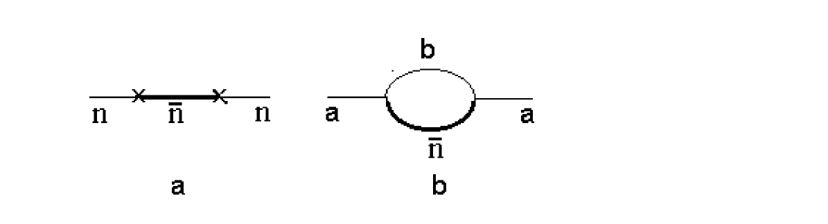
Figure 3: (a) The on-diagonal matrix element $T_{ii}$ corresponding to the $n\bar{n}$ transition in the medium. The Hamiltonian of the $\bar{n}$-medium interaction is given by eq. (3). (b) The same as (a) for the decay $a\rightarrow b\bar{n}$.

To clarify the structure of (10), we consider the same problem by means of a diagram technique [1] (see fig. 3a). Here we use the $S$-matrix rather then an evolution operator. Put $U_{n}={\rm Re}U_{\bar{n}}=0$ for simplicity. The Hamiltonian (5) has the form

$${\cal H}_{I}=\epsilon\bar{\Psi}_{\bar{n}}\Psi_{n}+H.c.-i\frac{\Gamma}{2}\bar{\Psi}_{\bar{n}}\Psi_{\bar{n}}.$$ (12)

The antineutron propagator $G$ and total process probability $W_{t}^{d}(t)$ are

$$G=1/(\epsilon_{n}-{\bf p}^{2}/2m+i\Gamma/2)=2/i\Gamma,$$

$$W_{t}^{d}(t)=-2{\rm Im}\epsilon G\epsilon t=\frac{4\epsilon^{2}t}{\Gamma},$$ (13)

where $p=(\epsilon_{n},{\bf p})$ is the neutron 4-momentum; $\epsilon_{n}={\bf p}^{2}/2m$. So $W_{t}^{d}=W_{t}$, where $W_{t}$ is given by (10). The $\Gamma$-dependence of $W_{t}$ is conditioned by the propagator $G$. This fact is common for a 2-tail diagram (fig. 3a) and diagrams with a momentum transferred $q\neq 0$ (figs. 1b, 3b and 4b).

In this section the standard scheme of calculation has been used. It is based on the Hamiltonian (5) and equation $W_{t}=2{\rm Im}T_{ii}$. This is the sole way of calculation of $W_{t}$ in a one-particle model. For brevity, this model will be denoted as model (5). We, thus, see that (5) realized by means of the equations of motion or diagram technique contradicts to inequality (6).

4 Free-space process

To avoid questions connected with the medium corrections, we consider the imaginary free-space process

$$n\rightarrow\bar{n}\rightarrow\bar{p}e^{+}\nu,$$ (14)

in which the neutron decay is excluded. The hermitian Hamiltonian is ${\cal H}_{I}=\epsilon\bar{\Psi}_{\bar{n}}\Psi_{n}+H.c.+{\cal H}_{h}^{\beta}$, where ${\cal H}_{h}^{\beta}$ is the Hamiltonian of the free-space $\beta^{+}$-decay $\bar{n}\rightarrow\bar{p}e^{+}\nu$. The corresponding diagram is shown in fig. 4a.

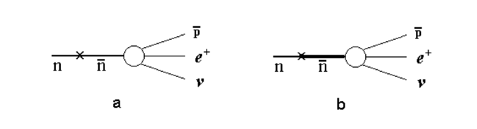
Figure 4: (a) The free-space process $n\rightarrow\bar{n}\rightarrow\bar{p}e^{+}\nu$. (b) The diagram corresponding to the effective amplitude of the process (14) (see the text).

Alternatively, if we want to use model (5), we have

$${\cal H}_{I}=\epsilon\bar{\Psi}_{\bar{n}}\Psi_{n}+H.c.-i\frac{\Gamma_{\beta}}{2}\bar{\Psi}_{\bar{n}}\Psi_{\bar{n}},$$ (15)

where $\Gamma_{\beta}$ is the width of the free-space $\beta^{+}$-decay $\bar{n}\rightarrow\bar{p}e^{+}\nu$. Comparing with (12), it is seen that we can use all the formulas given above in which $\Gamma=\Gamma_{\beta}$. The total probability of the free-space $n\bar{n}$ transition $W_{t}^{\beta}$ is given by (10) or (13):

$$W_{t}^{\beta}(t)=-2{\rm Im}\epsilon G\epsilon t\approx 4\epsilon^{2}t/\Gamma_{\beta},$$ (16)

$\Gamma_{\beta}t\gg 1$. The free-space $n\bar{n}$ conversion is drastically suppressed by the decay in the final state. Indeed, the free-space $n\bar{n}$ transition probability $W_{f}$ is $W_{f}=\epsilon^{2}t^{2}$ (see (11), where $\Gamma=0$) and correspondingly $W_{t}^{\beta}(t)/W_{f}(t)\sim 1/\Gamma_{\beta}t\ll 1$. This is clearly wrong because the state the of intermediate $\bar{n}$ (see fig. 4a) coincides with the final state of the free-space $n\rightarrow\bar{n}$ transition, and so the $\beta^{+}$-decay makes no influence on the subprocess of the $n\bar{n}$ conversion. This is sufficient to reject the model (5).

We should make a small comment. The process shown in fig. 4a represents two consecutive free-space subprocesses. The speed and probability of the overall process are defined by those of the slower subprocess. Since $1/\Gamma_{\beta}\ll t$, the $\beta^{+}$-decay can be considered instantaneous: for any $t_{1}<t$ the $\beta^{+}$-decay probability $W_{\beta}$ is $W_{\beta}(t_{1},t)\approx 1$. Then, the total process probability $W^{\beta}$ is defined by the speed of the $n\bar{n}$ conversion: $W^{\beta}\approx W_{f}\sim t^{2}$ instead of $W_{t}^{\beta}\sim t/\Gamma_{\beta}$.

Let us try to compose an effective model which produces $W_{t}^{\beta}$ through the direct calculation of the off-diagonal matrix element. We consider fig. 4b. It differs from fig. 4a by the fact that the antineutron is in the potential $V=-i\Gamma_{\beta}/2$. (Nonsense, of course.) The process amplitude is $M_{eff}=-\epsilon GM_{\beta}$, $G=-1/V$, where $M_{\beta}$ is the amplitude of the $\beta^{+}$-decay. For the process width we have $\Gamma_{eff}=\int d\Phi\mid\!M_{eff}\!\mid^{2}/2m=4\epsilon^{2}/\Gamma_{\beta}$, which coincides with $W_{t}^{\beta}/t$. So we have fixed $<\!f|=<\!\bar{p}e^{+}\nu|$ and found that the effective amplitude of process (14) which produces the result (16), is given by fig. 4b.

The fallacy of this model is obvious. Certainly, this is an illustration only, but structure (16) can be obtained by means of the Green function $G=-1/V\sim 1/\Gamma$ solely.

In the calculation of the $W_{t},W_{t}^{d}$ and $W_{t}^{\beta}$ model (5) is used. The result $W_{t}\sim 1/\Gamma$ is very sensitive to $\Gamma$. However, the $\Gamma$-dependence of $W_{t}$ contradicts to inequality (6). Besides, result (16) is unrealistic. Therefore, this model should be revised.

5 Unitarity and self-energy

In this and next sections the reasons for disagreement indicated above are studied. If $\Gamma=0$, system (7) is certainly correct. Consequently, it is necessary to revise the role of $i{\rm Im}U_{\bar{n}}$. This question has been considered in [1]. Taking into account the importance of this problem, we adduce more direct evidence using the $U(t)$-operator only. The approach based on the evolution operator is more general than the $S$-matrix one, since in this case the time-dependence of the process does not need to be $W_{t}=1-\exp(-\Gamma_{t}t)$ (see (8)). Also it is infrared-free, which is essential for $ab$ transitions [13].

The non-hermiticity of ${\cal H}$ implies that

$$(U(t)U^{+}(t))_{fi}=\delta_{fi}+\alpha_{fi}(t),$$ (17)

$\alpha_{fi}\neq 0$, resulting in

$$W_{t}(t)=\sum_{f\neq i}\mid T_{fi}(t)\mid^{2}\approx 2{\rm Im}T_{ii}(t)+\alpha_{ii}(t)\neq 2{\rm Im}T_{ii}(t)$$ (18)

because the value of $2{\rm Im}T_{ii}$ is extremely small:

$$2{\rm Im}T_{ii}(t_{0})=\frac{4\epsilon^{2}t_{0}}{\Gamma}<10^{-31},$$ (19)

where the standard set [1, 14-16] of parameters $\epsilon$, $t_{0}$ and $\Gamma$ has been used. We thus see that (8) is invalid.

For the $S$-matrix, the conclusions are the same: (a) The basic relation

$$\sum_{f\neq i}\mid T_{fi}\mid^{2}\approx 2{\rm Im}T_{ii}$$ (20)

is inapplicable. (b) The physical meaning of ${\rm Im}\Sigma=-\Gamma/2$ is uncertain because it is clarified using relation (20). We would like to emphasize this fact.

On the one hand, the $n\bar{n}$ transition probability is very small (see (19)), and on the other hand, the term $i{\rm Im}U_{\bar{n}}$ plays a crucial role because it enters the leading diagram (see (13)). Because of this for the problem under study the unitarity of the $S$-matrix is of particular importance.

Thus, the non-hermitian Hamiltonian (3) leads to inverse $\Gamma$-dependence of $W_{t}$ and to the imaginary self-energy. In QED the Green function above threshold contains an imaginary self-energy ${\rm Im}\Sigma\neq 0$ as well. However, in the case of QED the situation differs principally. ${\rm Im}\Sigma$ is a complicated function of parameters of the hermitian Hamiltonian. It appears at higher orders in $\alpha$. The width $\Gamma$ makes its appearance after a Dyson summation of the relevant self-energies. In order to correctly enforce unitarity, the notation of the ”running width” has been introduced.

The importance of unitarity condition is well known [17,18]. Nevertheless, the non-hermitian models (3)-(5) are frequently used for the reasons given in sect. 1. In particular, all existing calculations of $n\bar{n}$ transitions in the medium are based on model (5) (see, for example, [13] for future references).

With the substitution $i{\rm Im}U_{\bar{n}}=-i\Gamma_{x}/2$, where $\Gamma_{x}$ is a width of some free-space decay $\bar{n}\rightarrow x$, the Green function (13) describes the non-relativistic resonance; Hamiltonians (4) and (5) correspond to the free-space two-step processes: $a\rightarrow b+\bar{n}\rightarrow b+x$ and $n\rightarrow\bar{n}\rightarrow x$, respectively. This is obvious because the absorption can be considered as the decay of a one-particle state. Formally, in these cases all the results are also true. Nevertheless, the resonances invite an additional consideration. As far back as 1959, M. Levy remarked that there does not exist a rigorous theory to which various phenomenological methods of treating resonances and decays can be considered as approximations [19]. Attempts have been made at an axiomatic theory [20,21].

The above-mentioned difficulties take place for absorption as well. These conceptual problems are beyond the scope of this paper. We deal with concrete models (3)-(5) and hence propagator (13) because they are frequently used. As for resonances and decays, we only draw the formal analogy between absorption Hamiltonian (3) and phenomenological Hamiltonian of decay $-i\Gamma/2\bar{\Psi}\Psi$.

We also note that decay (14) can be calculated by means of the usual field-theoretical approach, but the problem should be formulated on the finite time interval [22] since fig. 4a contains an infrared singularity.

6 Optical potential

The problem is not only in the unitarity. It is in the correct description of the absorption on the whole. In the theory of optical potential $i{\rm Im}U$ is non-hermitian as well. However, the picture differs principally in this case. In this section we compare the equation of motion and the problem under study from the standpoint of the use of an optical potential.

In the case of Schrodinger equation

$$(i\partial_{t}-H_{0}-U_{\bar{n}})\bar{n}=0$$ (21)

the scheme is as follows. Since $U_{\bar{n}}$ is non-hermitian, the condition of probability conservation

$$1=\mid U_{ii}\mid^{2}+W_{{\rm Sch}}$$ (22)

is imposed. Here $W_{{\rm Sch}}$ is the loss of $\bar{n}$ intensity. The matrix element of evolution operator is found to be

$$U_{ii}(t)=<\bar{n}(0)\mid\bar{n}(t)>=e^{-i{\rm Re}U_{\bar{n}}t}e^{{\rm Im}U_{\bar{n}}t}.$$ (23)

From (22) and (23) it is seen that: (a) $W_{{\rm Sch}}\neq 0$ if and only if ${\rm Im}U_{\bar{n}}<0$ (or $\Gamma>0$, when ${\rm Im}U_{\bar{n}}=-\Gamma/2$). (b) If $\Gamma$ increases, $W_{{\rm Sch}}$ increases as well:

$$\frac{{\rm d}W_{{\rm Sch}}}{{\rm d}\Gamma}=\frac{{\rm d}}{{\rm d}\Gamma}(1-e^{-\Gamma t})>0.$$ (24)

This agrees with (6) and is in contradiction with (10), (11) and (16).

The procedure given above is based on two points: 1) In (21) ${\rm Im}U_{\bar{n}}$ has a clear physical meaning. It is defined by the continuity equation corresponding to (21). 2) The additional bound (22) provides the probability conservation (unitarization). By means of (21) and (22) $U_{\bar{n}}$ is fitted to the $\bar{p}$-atom and low energy scattering data.

For more complex problems these requirements, as a rule, are not fulfilled. We demonstrate this for model (5). The fit of (7) and (8) is impossible since there are no experimental data. As a result we have (18) with the consequences considered above. In addition, we try to realize the scheme given for (21).

The coupled eqs. (7) give rise to the following equation

$$(\partial_{t}^{2}+i\partial_{t}(V+2H_{0})-H_{0}^{2}-H_{0}V+\epsilon^{2})n(x)=0.$$ (25)

According to (8), $n(x)$ is sufficient to get $W_{t}$.

Even the first step of the scheme described above is not realized: one cannot get the continuity equation from (25). The $S$-matrix consideration accomplishes nothing because eq. (20) is inapplicable.

Equations (7), i.e. model (5), describe only $W_{\bar{n}}$. In this case $U_{\bar{n}}$ can be included in the distorted wave of the antineutron which is the eigenfunction of eq. (21), and this justifies the model.

7 Generalization

If instead of Hamiltonian (5) we take

$${\cal H}_{I}={\cal H}_{r,d}+{\cal H},$$ (26)

where ${\cal H}_{r}$ and ${\cal H}_{d}$ correspond to free-space reaction and decay, respectively, the qualitative conclusions do not change because the heart of the problem is in the Hamiltonian ${\cal H}$. As an example, let us consider the decay $a\rightarrow b\bar{n}$ in the medium. Let $\Gamma_{\bar{n}}$ and $\Gamma_{a}$ be the widths of decays with $\bar{n}$ and the annihilation mesons in the final state, respectively; $\Gamma_{t}$ is the total decay width, $\Gamma_{t}=\Gamma_{\bar{n}}+\Gamma_{a}$. The corresponding partial decay probabilities are $W_{\bar{n},a}\approx\Gamma_{\bar{n},a}t$. $W_{\bar{n}}$ and $W_{a}$ are the same as in sect. 2. To draw the analogy to $n\bar{n}$ transitions, we use the probabilities $W$.

Equations (7) are time-dependent and so the evolution operator has been applied. For the decays the $S$-matrix is used. In (18) one should replace $T(t)\rightarrow T$. The interaction Hamiltonian is given by (4). We have

$$\Gamma_{t}=\frac{2}{T_{0}}{\rm Im}T_{ii},$$ (27)

where $T_{0}$ is the normalization time, $T_{0}\rightarrow\infty$. The matrix element $T_{ii}$ is shown in fig. 3b. In principle, the antineutron propagator in the loop should be calculated through the hermitian Hamiltonian ${\cal H}_{a}$: $G=G({\cal H}_{a})$. Model (4) means that

$$G({\cal H}_{a})\rightarrow G({\cal H})=G(-i\Gamma/2)=-\frac{1}{\hat{p}_{\bar{n}}-m+i\Gamma/2},$$ (28)

where $p_{\bar{n}}$ is the antineutron 4-momentum. Obviously, for the matrix element shown in fig. 3b eq. (18) takes place as well. Relation (20) is invalid; the physical meaning of ${\rm Im}\Sigma=-\Gamma/2$ is uncertain.

The probability of finding an antineutron $W_{\bar{n}}$ is described by an off-diagonal matrix element. In the distorted wave impulse approximation the interaction responsible for the absorption is included in the antineutron wave function:

$$\bar{n}(x)=\Omega^{-1/2}e^{-i[({\bf p}^{2}/2m+i{\rm Im}U)t-{\bf p}{\bf x}]}.$$ (29)

The corresponding diagram is shown in fig. 1a, where the antineutron state is described by (29). The wave function $\bar{n}(x)$ is the eigenfunction of eq. (21), which justifies the using of model (3) in the calculation of $\bar{n}(x)$ and $W_{\bar{n}}$.

The probability of finding the annihilation products is obtained from

$$W_{a}=W_{t}-W_{\bar{n}}.$$ (30)

Since eqs. (20) and (27) are inapplicable, $W_{t}$ and $W_{a}$ are uncertain.

We thus see that (4) describes only $W_{\bar{n}}$. The result is the same as for the $n\bar{n}$ transitions considered above. Obviously, in the strong absorption region $W_{\bar{n}}\ll W_{a}$ and $W_{\bar{n}}\ll W_{t}$.

Figures 1b and 2b correspond to absorption in the final state. Model (3) is also used for the description of the absorption in the intermediate state (see fig. 5). The interaction Hamiltonian of the process shown in fig. 5 has the form

$${\cal H}_{I}={\cal H}_{1}+{\cal H}+{\cal H}_{h}^{\beta}.$$ (31)

The quantitative study of models (26) and (31) is subject of a separate investigation. Here we consider only a qualitative picture. The amplitude corresponding to fig. 5 is given by

$$T_{5}=-M_{1}G(i\Gamma)M_{\beta},$$

$$G(i\Gamma)=[(p_{0}-q_{0}-m)-({\bf p}-{\bf q})^{2}/2m+i\Gamma/2]^{-1}.$$ (32)

Here $M_{1}$ and $M_{\beta}$ are the amplitudes of decay (1) and $\beta^{+}$-decay, respectively; $p$ and $q$ are the $4$-momenta of particles $a$ and $b$, respectively; $m$ is the antineutron mass.

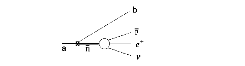
Figure 5: The decay $a\rightarrow b+\bar{n}\rightarrow b+\bar{p}+e^{+}+\nu$ in the medium. The bold line signifies the antineutron annihilation in the intermediate state.

The antineutron propagator $G({\cal H}_{a})$, calculated through the hermitian Hamiltonian ${\cal H}_{a}$, contains the loops. This leads to suppress the amplitude $T_{5}$. $G(i\Gamma)$ from (32) acts in the same direction: the probability of finding the $\beta^{+}$-decay products is $W_{5}\sim\Gamma_{\beta}/\Gamma^{2}$. $W_{5}$ is less sensitive to model (3) than $W_{t}$ because the unitarity condition is not used. In this case at least there is no qualitative contradiction. (This question needs quantitative consideration. Most likely model (32) yields too great suppression.)

Below we consider the most realistic case $\Gamma\gg\Gamma_{\beta}$. In the lowest order in ${\cal H}_{h}^{\beta}$ the probability of finding an antineutron $W_{\bar{n}}$ is the same as for Hamiltonian (4). For the on-diagonal matrix element $T_{ii}$ and total decay probability $W_{t}$ the calculation scheme and conclusions are also identical to those for (4) and (26). The fact that the antineutron propagator in the loop is defined by ${\cal H}_{h}^{\beta}$ and ${\cal H}$ is not principal because the heart of the problem is in the $i{\rm Im}U_{\bar{n}}$.

Similarly to (30) we have

$$W_{a}=W_{t}-W_{\bar{n}}-W_{5}.$$ (33)

Since eq. (20) is inapplicable, $W_{t}$ and $W_{a}$ are uncertain.

For model (31) we conclude: (a) $W_{\bar{n}}$ should be described correctly. (b) The major decay characteristics $W_{t}$ and $W_{a}$ are not described. (c) For the process shown in fig. 5 model (32) can be used as a first approximation.

8 Unitary model

In sects. 2-4 on the basis of a general reasoning we concluded that in the phenomenological model the $\Gamma$-dependence of $W_{t}$ is wrong. Below we consider the unitary model and calculate directly the off-diagonal matrix element by means of the diagram technique.

If $\Gamma t\gg 1$, the probability of finding an annihilation mesons $W_{a}$ is much greater than $W_{\bar{n}}$. However, the phenomenological model describes $W_{\bar{n}}$ only. Recall that for the total $n\bar{n}$ transition probability the phenomenological model gives $W_{t}\sim 1/\Gamma$ (see (13)). Since $W_{\bar{n}}\ll W_{t}$, $W_{a}$ depends inversely on $\Gamma$ as well:

$$W_{a}=W_{t}-W_{\bar{n}}\approx W_{t}\sim 1/\Gamma.$$ (34)

For the processes which are described by Hamiltonians (26) and (31) it is sufficient to recall that the $W_{t}$ and $W_{a}$ are uncertain for the reasons given above. In our opinion, with correct consideration of the corresponding loops we will obtain ${\rm d}W_{t}/{\rm d}\Gamma<0$, as with (34).

The direct calculation of off-diagonal matrix element gives the inverse $\Gamma$-dependence ${\rm d}W/{\rm d}\Gamma>0$. Indeed, we consider the process (1). The $a$-particle and $\bar{n}$ are assumed non-relativistic. The wave function of the $b$-particle is $\Phi_{b}(x)=(2q_{0}\Omega)^{-1/2}\exp(-iqx)$, where $q$ is the 4-momentum of the particle. As with ${\cal H}_{n\bar{n}}$, the decay Hamiltonian is taken in the scalar form ${\cal H}_{1}=\epsilon^{\prime}\bar{\Psi}_{\bar{n}}\Phi^{*}_{b}\Psi_{a}+H.c.$ and correspondingly

$${\cal H}_{I}=\epsilon^{\prime}\bar{\Psi}_{\bar{n}}\Phi^{*}_{b}\Psi_{a}+H.c.+{\cal H}_{a};$$ (35)

$\epsilon^{\prime}$ is dimensionless.

The process amplitude is given by

$$M_{1}=-\epsilon^{\prime}\frac{1}{(p_{0}-q_{0}-m)-({\bf p}-{\bf q})^{2}/2m+i0}M_{a}.$$ (36)

Here $M_{a}$ is the annihilation amplitude, $m$ is the antineutron mass, $p$ is the 4-momentum of the $a$-particle.

For simplicity assume that $m_{b}/m\ll 1$, where $m_{b}$ is the mass of the $b$-particle. It is easy to estimate the width of decay (1):

$$\Gamma_{1}\approx\epsilon^{\prime 2}\Gamma/(2\pi^{2}).$$ (37)

The corresponding decay probability is proportional to $\Gamma$:

$$W_{a}^{h}=\Gamma_{1}t\sim\Gamma.$$ (38)

The index $h$ signifies that the hermitian Hamiltonian is used.

The width of process (2) is also linear in $\Gamma$ [1]:

$$\Gamma_{2}\sim\Gamma.$$ (39)

For the Hamiltonians containing three terms the $\Gamma$-dependence of $W_{a}^{h}$ is the same. Thus,

$$W_{a}^{h}\sim W_{t}^{h}\sim\Gamma,$$ (40)

where $W_{t}^{h}$ is the total process probability.

From eqs. (40) and (34), we see that the unitary and non-unitary models lead to inverse $\Gamma$-dependence of the results. Because of this the calculations with the hermitian ${\cal H}_{a}$ can tend to increase $W_{a}$ and $W_{t}$. (See also eq. (12) of ref. [1].)

9 Summary and conclusion

We list the consequences of an unjustified use of the model based on eqs. (20) and (3).

1) Equation (9) contradicts to (6) and (24).

2) Result (16) is unrealistic.

3) $W_{t}\sim 1/\Gamma$, whereas $W^{h}_{t}\sim\Gamma$ (see (34) and (40)).

4) The physical meaning and value of the ${\rm Im}\Sigma$ are uncertain (see text below (20)).

Model (3) was adapted to quite definite problems. It is justified for the problems described by Schrodinger type equations. It also describes the complicated processes (reactions, decays and $n\bar{n}$ transitions) with $\bar{n}$ in the final state. (More formally, model (3) can be applied to the calculation of $W_{\bar{n}}$ corresponding to the Hamiltonians containing several terms (eqs. (26) and (31), for example).) As a first approximation, it can be used in the calculation of the diagrams like that shown in fig. 5 with $\bar{n}$ in the intermediate state. In these cases $W$ are calculated directly without the use of the unitarity condition and the calculation of $T_{ii}$.

In other cases, when the interaction Hamiltonian contains several terms and the unitarity condition is used (eqs. (8), (13), (27) and (33), for example), model (3) is inapplicable. The calculation of the total process probability $W_{t}$ (and thus $W_{a}$) corresponding to inclusive reaction, decay or $ab$ transition is impossible. The physical meaning of ${\rm Im}\Sigma$ is uncertain. The effect of absorption, as a rule, acts in the opposite (wrong) direction, which leads to additional suppression. In particular, model (5) gives rise to the dramatic suppression of $n\bar{n}$ transitions due to the annihilation in the final state, which is wrong.

This paper also demonstrates the importance of the unitarity condition for any model of $\Sigma$ [23,24]. The model should by unitary or unitarized.

Finally, we touch upon the result sensitivity to model (3). It is seen from the Green function (32). The $\Gamma$-dependence is masked by $q$. If $q\rightarrow 0$ (2-tail) and $m_{a}=m$, the problem is extremely sensitive to $\Gamma$: $T_{5}\sim 1/\Gamma$. Alternatively, in the phenomenological model the $n\bar{n}$ conversion is described by system (7) which has an exact solution. For these reasons the $n\bar{n}$ transitions in the medium are the ideal instrument for the study of the final state absorption.

We also emphasize the following: the absorption (decay) in the final state (figs. 1b, 2b and 4a, for example) does not lead to suppress the total process probability as well as the probability of the channel corresponding to absorption, in contrast to the phenomenological model results. Therefore, the calculations based on unitary models can tend to increase the above-mentioned values.

The author is grateful to Prof. E. Oset for helpful comments.

References

- [1] V.I. Nazaruk, Mod. Phys. Lett. A 21, 2189 (2006); V.I.Nazaruk, Proceedings of the 9th International Conference on Low Energy Antiproton Physics (LEAP’05), Bonn, Germany 2005, edited by D.Grzonka, R. Czyzykiewich, W.Oelert, T.Rozek, P.Winter, AIP Conf. Proc. Vol. 796, p.180 (2005).
- [2] M. Feshbach, C.E. Porter, and V.F. Weisskopf, Phys. Rev. 90, 166 (1953); 96, 448 (1954); T. Ericson and W. Weise, Pions and Nuclei (Clarendon Press, Oxford, 1988).
- [3] V.A. Kuzmin, JETF Lett. 12, 228 (1970); S.L. Glashow, preprint HUTP-79/A059 (Harvard, 1979) unpublished.
- [4] R.N. Mohapatra and R.E. Marshak, Phys. Rev. Lett. 44, 1316 (1980).
- [5] K.G. Chetyrkin, M.V. Kazarnovsky, V.A. Kuzmin and M.E. Shaposhnikov, Phys. Lett. B 99, 358 (1981).
- [6] N. Austern, Direct Nuclear Reaction Theories (N.Y., Wiley-Interscience, 1970).
- [7] A. Bieniek et al., Phys. Lett. B 526, 329 (2002); M. Benmerrouche et al., Phys. Rev. C 39, 2339 (1989).
- [8] V.K. Madas, L. Roka and E. Oset, Phys. Rev. C 71, 065202 (2005).
- [9] M.L. Good, Phys. Rev. 106, 591 (1957).
- [10] L. Wolfenstein, Phys. Rev. D 17, 2369 (1978).
- [11] P.G.H. Sandars, J.Phys. G6, L161 (1980).
- [12] W.M. Alberico et al., Nucl. Phys. A 523, 488 (1991).
- [13] V.I. Nazaruk, Phys. Rev. C 58, R1884 (1998).
- [14] H. Takita et al., Phys. Rev. D 34, 902 (1986).
- [15] V.I. Nazaruk, Yad. Fiz. 56, 153 (1993).
- [16] M. Baldo-Ceolin et al., Phys.Lett. B 236, 95 (1990).
- [17] T. Inone and E. Oset, Nucl. Phys. A 710, 354 (2002); 721, 661 (2003).
- [18] E. Oset, Nucl. Phys. A 721, 58 (2003).
- [19] M. Levy, Nuovo Cimento 13, 115 (1959).
- [20] A. Bohm and N.L. Harshman, Nucl. Phys. B 581, 91 (2000).
- [21] A. Bohm et al., Fortschr. Phys. 51, 599 (2003); 604 (2003).
- [22] V.I. Nazaruk, Phys. Lett. B 337, 328 (1994).
- [23] P. Fernandez de Cordona and E. Oset, Phys. Rev. C 46, 1697 (1992).
- [24] L. Alvarez-Ruso, P. Fernandez de Cordoba and E. Oset, Nucl. Phys. A 606, 407 (1996).