Nucleon decay in gauge unified models with intersecting $D6$-branes

Abstract

Baryon number violation is discussed in gauge unified orbifold models of type II string theory with intersecting Dirichlet branes. We consider setups of $D6$-branes which extend along the flat Minkowski space-time directions and wrap around 3-cycles of the internal 6-d manifold. Our study is motivated by the enhancement effect of low energy amplitudes anticipated for M-theory and type $II$ string theory models with matter modes localized at points of the internal manifold. The conformal field theory formalism is used to evaluate the open string amplitudes at tree level. We study the single baryon number violating processes of dimension $6$ and $5$, involving four quarks and leptons and in supersymmetry models, two pairs of matter fermions and superpartner sfermions. The higher order processes associated with the baryon number violating operators of dimension $7$ and $9$ are also examined, but in a qualitative way. We discuss the low energy representation of string theory amplitudes in terms of infinite series of poles associated to exchange of string Regge resonance and compactification modes. The comparison of string amplitudes with the equivalent field theory amplitudes is first studied in the large compactification radius limit. Proceeding next to the finite compactification radius case, we present a numerical study of the ratio of string to field theory amplitudes based on semi-realistic gauge unified non-supersymmetric and supersymmetric models employing the $Z_{3}$ and $Z_{2}\times Z_{2}$ orbifolds. We find a moderate enhancement of string amplitudes which becomes manifest in the regime where the gauge symmetry breaking mass parameter exceeds the compactification mass parameter, corresponding to a gauge unification in a seven dimensional space-time.

I INTRODUCTION

By suggesting the possibility that the Standard Model (SM) gauge and gravitational interactions unify in a higher dimensional space-time, string theory witten85 ; hetunif has opened up novel perspectives for the gauge unification proposal gsw . Based on the approach of Calabi-Yau (CY) manifold compactification, the string theory applications focused initially on the heterotic string in the regimes of weak coupling arno8594 and strong coupling Mtheory96 ; witten96 ; kapcac97 ; ovrut99 . These studies were soon followed by explicit constructions using orbifold compactification aldaz95 ; kakush97 and free fermion ellisfar97 models of the heterotic string, which were later extended to orbifold compactification models of the type $II$ string theories with single $Dp$-branes lykken98 or the $Dp/Dp^{\prime},\ [p^{\prime}\neq p]$ branes-inside-branes type backgrounds tyegut98 .

The chief distinctive features of string gauge unification reside in the discrete gauge symmetry breaking scheme by Wilson flux lines ovrut85 and the heavy string threshold effects kap88 . Regarding, however, the issue of matter instability caused by baryon number violation, it is fair to say that no specific stringy effect has emerged from the earlier studies using the weakly coupled heterotic and type $II$ string theories. A different situation seems to take place in the 11-d M-theory supersymmetric compactification on 7-d internal manifolds $X_{7}$ of $G_{2}$ holonomy achar04 , as discussed by Friedman and Witten friedman02 . The non-Abelian gauge symmetries in these models are supported on 7-d sub-manifolds, $B=M_{4}\times Q$, loci for $R^{4}/\Gamma$ orbifold type singularities in the directions transverse to $B$, while the chiral massless fermions are supported at isolated singularities of the 3-d sub-manifolds, $Q$. This causes the existence of a natural regime where the grand unification occurs in a 7-d dimensional space-time with localized matter fermions. In comparison to the nucleon decay amplitudes of the equivalent unified gauge field theories, the string amplitudes are enhanced by a power $\alpha_{X}^{-{1\over 3}}$ of the unified gauge coupling constant, which reflects on the short distance singularities from summing over the momentum modes propagating in the sub-manifold $Q$. As to the size of the enhancement effect, however, no definite conclusions could be drawn because of the poor understanding of M-theory perturbation theory, not mentioning the greater complexity of $G_{2}$ holonomy manifolds revachar04 .

Fortunately, it is possible to examine the enhancement effect in a controlled way by considering the weak coupling dual models based on type $IIa$ string theory orientifold compactification on $M_{4}\times X_{6}$ with $D6$-branes wrapped around intersecting three-cycles of the internal Calabi-Yau complex threefold, $X_{6}$. Using a toy model realizing $SU(5)$ gauge unification, Klebanov and Witten KW03 showed that the four fermion string amplitude for localized matter modes in the gauge group representations, $10\cdot{10}^{\dagger}\cdot 10\cdot{10}^{\dagger}$, featured a power dependence on the unified gauge coupling constant of same form as in the M-theory model, namely, ${\cal A}\propto\alpha_{X}^{2/3}$. In the most favorable case where the fermion modes sit at coincident intersection points of the $D$-branes, the enhancement due to the gauge coupling constant dependence was found to be offset by certain constant factors which resulted in a rather modest net effect.

Our goal in the present work is to document the enhancement of string amplitudes anticipated in M-theory friedman02 by developing further semiquantitative calculations in models with intersecting $D$-branes. The initiating discussion in Ref. KW03 made use of the large compactification radius limit in which predictions are largely insensitive to the Wilson line mechanism responsible for the unified gauge symmetry breaking. We extend this study in three main directions. First, we consider semi-realistic orbifold-orientifold models realizing the $SU(5)$ gauge unification with a chiral spectrum of massless matter modes that closely reproduces the Standard Model spectrum. Second, we evaluate the nucleon decay four point amplitudes in the two independent configurations of gauge group matter representations, $10\cdot{10}^{\dagger}\cdot 10\cdot{10}^{\dagger}$ and $10\cdot\bar{5}\cdot 10^{\dagger}\cdot\bar{5}^{\dagger}$. which contribute to the proton two-body decay channels with emission of left and right helicity positrons, $p\to\pi^{0}+e^{+}_{L,R}$. This allows us to quantitatively assess the M-theory prediction for the ordering of partial decay rates, $\Gamma(p\to\pi^{0}+e^{+}_{L})>>\Gamma(p\to\pi^{0}+e^{+}_{R})$. Third, we discuss the string amplitudes at finite compactification radii, in order to weigh the importance of the string momentum and winding excitations relative to the string Regge resonances. Studying the interplay between the compactification and unified symmetry breaking mass scale parameters, $M_{c}$ and $M_{X}$, proves crucial in assessing the size of the enhancement effect.

The contributions to nucleon decay processes from physics at high energy scales are conveniently represented by non-renormalizable local operators in the quark and lepton fields weinbergs ; wilczee which violate the baryon and lepton numbers, $B,\ L$. In unified gauge theories, the exchange of massive gauge bosons with leptoquark quantum numbers induces in the effective action, $(B+L)$ violating, $(B-L)$ conserving operators of dimension ${\cal D}=6$. In supersymmetry models, the exchange of massive color triplet matter higgsino like modes also induces dangerous operators in the quark and lepton superfields of dimension ${\cal D}=5$. Higher dimension operators initiating the exotic nucleon decay processes can possibly arise from mass scales significantly lower than the gauge interactions unification scale, $M_{X}\simeq 3.\times 10^{16}$ GeV. Of special interest are the $B-L$ violating operators of dimension ${\cal D}\geq 7$, and the double baryon number violating operators of dimension ${\cal D}\geq 9$, responsible for nucleon-antinucleon oscillation.

The 2-d conformal quantum field theory polchb provides a powerful approach for calculating the on-shell string theory amplitudes. The construction of string amplitudes cftopen from vacuum correlators of open string vertex operators inserted on the world sheet disk boundary is readily applied to the 4-d amplitudes describing the nucleon decay processes. The tree level contributions to the dimension ${\cal D}=6,\ 5$ operators involve four fermions, $\psi^{4}$, or two pairs of fermions and bosons, $\psi^{2}\phi^{2}$. For the intersecting brane models with matter modes localized in the internal directions, the calculations are made non-trivial by the need to account for the twisted like boundary conditions of the world sheet fields. Fortunately, the energy source approach, which was initially invented bersh87 ; dixon87 ; dixontasi ; cohn86 ; zam87 and subsequently developed burwick ; orbifhet ; bailin93 in the context of closed string twisted sectors of orbifolds, can be readily extended to the localized open string sectors of intersecting brane models. Following previous studies devoted to the discussion of open string modes with mixed ND boundary conditions in $Dp/Dp^{\prime}$-brane models hashi96 ; gava97 ; fro099 ; antbengier01 , the implementation of this approach for intersecting brane models has been clarified in discussions by Cvetic and Papadimitriou Cvetic:2003ch , Abel and Owen owen03 , Klebanov and Witten KW03 , Jones and Tye jones03 , Lüst et al., luststie04 and Antoniadis and Tuckmantel antontel04 . A comprehensive review of the first quantization and conformal field theory formalisms for the open string string sectors of $D$-brane models is currently under preparation chemnd05 . We should also mention here the studies by Billo et al., billo02 , Bertolini et al., bertol05 , and Russo and Sciuto, russo07 which develop the alternative approach based on the operator formalism.

An intense activity has been devoted in recent years to the discussion type $II$ string theory compactification using intersecting $D$-brane backgrounds berk96 ; balasub97 ; arfaei97 . To be complete, we should mention the parallel development on T-dual $D$-brane models using magnetised backgrounds bachas95 ; antonti00 and on the magnetic field deformations of the heterotic string witten84 . Important efforts towards building satisfactory models have been spent in works by Aldazabal et al., aldaisb01 ; iban0 ; iban1 ; ibanyuk ; iban2 ; cimmag04 , Kokorelis kokosusy02 ; kokogut02 ; kokor02 , Blumenhagen et al., Blumenhagen:1999md ; Blumenhagen:1999db ; Blumenhagen:1999ev ; Blumenhagen:2000ea ; Blumenhagen:2000fp ; Blumenhagen:2000wh ; Blumenhagen:2001te ; Blumenhagen:2001mb , and Cvetic et al., Cvetic:2001nr ; Cvetic:2001tj ; Cvetic:2002pj ; Cvetic:2003xs ; Cvetic:2004ui ; Cvetic:2005lll ; cvet06 . A useful review is presented in Ref. blumshiu05 . To develop our applications in the present work, we consider semi-realistic models already discussed in the literature. First, we should note that the minimal toroidal orientifold models developed by Cremades et al., iban1 ; ibanyuk ; iban2 are of little use to us in the present work, because these realize direct compactifications to the Standard Model (SM), the minimal supersymmetric Standard Model (MSSM) iban1 ; ibanyuk ; iban2 , or the Pati-Salam type unified model kokogut02 , which all accommodate a built-in $U(1)_{B+L}$ global symmetry which guarantees $B$ and $L$ number conservation. A better answer to our needs is provided by the orbifold models Blumenhagen:1999md ; Blumenhagen:1999db ; Blumenhagen:2001te ; Blumenhagen:2001mb ; Cvetic:2001nr ; Cvetic:2001tj ; Cvetic:2002pj ; Cvetic:2003xs ; Cvetic:2004ui ; honeck01 ; honeck02 ; ellis03 ; blumz402 ; blumlust02 ; blumlonsu04 ; honec03 ; honec04 ; axeni03 ; kokor04 owing to their richer structure and more constrained character. We have selected the two classes of non-supersymmetric and supersymmetric gauge unified models realizing a minimal type $SU(5)$ gauge unification. The first class relates to the works of Blumenhagen et al., Blumenhagen:2001te and Ellis et al., ellis03 using the $Z_{3}$ orbifold, and the second class to the work of Cvetic et al., Cvetic:2001nr using the $Z_{2}\times Z_{2}$ orbifold. It is important to emphasize at this point that the calculation of string amplitudes relies on features of the non-chiral mass spectrum and the wave functions of low-lying modes which are not directly addressed in these works. For instance, the application to $Z_{3}$ orbifold models rely on data involving the real wrapping numbers rather than the effective ones which are defined by summing over the orbifold group orbits.

The discussion in the present paper is organized into five sections. In Section II, we review the first quantization and conformal field theory formalisms for type $II$ orientifold models with intersecting $D6$-branes. The open string sectors are discussed first for tori and next for orbifolds. A review of the energy source approach for calculating the correlators of coordinate twist field operators is provided in Appendix A. In Section III, we discuss the calculation of string amplitudes for nucleon decay processes in the gauge unified models. The world sheet disk amplitudes are considered in succession for the processes involving four massless fermions, two pairs of massless fermions and bosons, four massless fermions and a scalar, and six massless fermions. These are described by operators of dimension, ${\cal D}=6$ and $5$, ${\cal D}=7,$ and ${\cal D}=9$, obeying the selection rules, $\Delta B=\Delta L=-1$, $\Delta B=-\Delta L=-1$ and $\Delta B=-2,\ \Delta L=0$. In Section IV, we discuss the relations linking the low energy gauge and gravitational interaction coupling constants to the fundamental string theory parameters $g_{s}$ and $m_{s}$, and to the mass parameters representing the average compactification radius of wrapped three-cycles, $r=1/M_{c}$, and the unified gauge symmetry breaking, $M_{X}$, arising as an infrared mass cutoff. We consider in turn two distinct regularization procedures of the string amplitudes. The first uses the subtraction prescription replacing the massless pole terms by massive ones, and the second uses the displacement prescription splitting the unified $D$-brane into separated stacks. To illustrate the dependence of four fermion string amplitudes on the $D$-branes intersection angles, an initial numerical application is considered within the large compactification radius limit. However, the main thrust of the present work bears on the study of baryon number violating string amplitudes at finite compactification radius. The results illustrating the enhancement of nucleon decay string amplitudes are presented in Section V. We consider first the non-supersymmetric $SU(5)$ unified models of the $Z_{3}$ orbifold due to Blumenhagen et al., Blumenhagen:2001te and Ellis et al., ellis03 and next the supersymmetric $SU(5)$ unified model of the $Z_{2}\times Z_{2}$ orbifold due to Cvetic et al., Cvetic:2001nr . In Section VI, we summarize our main conclusions. For completeness, we provide a brief review of the $Z_{3}$ orbifold models in Appendix B and a brief review of baryon number violating processes for gauge unified theories in Appendix C.

II Review of type $II$ string orientifolds in intersecting $D6$-brane backgrounds

We present in this section a brief review of the open string sector of type $II$ string theory orientifolds with intersecting $D6$-branes. The first-quantized and vertex operators formalisms are discussed for toroidal compactification in Subsections II.1 and II.2 and for orbifold compactification in Subsection II.3.

II.1 Toroidal compactification

II.1.1 World sheet field theory

The Neveu-Schwarz-Ramond type $IIa$ string theory deals with 2-d world sheet Riemann surfaces on which live the coordinate and Majorana-Weyl 2-d spinor fields parameterizing the 10-d target space-time with signature $(-+\cdots+)$. For a flat space-time, one uses the diagonal representation of the metric tensor, $-\eta_{00}=\eta_{\mu\mu}=\eta_{mm}=1$, associated to the orthogonal field basis, $X^{M},\ \psi^{M},\ [M=(\mu,m)=0,1\cdots,9,\ \mu=0,1,2,3;\ m=4,5,6,7,8,9]$ with the complexified basis of coordinate fields, $X^{A},\ \bar{X}^{A},\ [A=0,1,\cdots,4]$ defined by

$$X^{M}=[X^{\mu};\ X^{m}]=[X^{\mu};\ X^{A},\bar{X}^{A}],\ [A=(a,0)=(I,4,0),\ I=1,2,3]$$ (II.1)

$$\bigg{[}X^{\pm}\equiv(X^{0},X^{\bar{0}})={X^{0}\pm X^{1}\over\sqrt{2}},\ (X^{4},X^{\bar{4}})={X^{2}\pm iX^{3}\over\sqrt{2}};$$ (II.2)

$$(X^{I},\ \bar{X}^{I})\equiv{X^{I}_{1}\pm iX^{I}_{2}\over\sqrt{2}}={X^{2I+2}\pm iX^{2I+3}\over\sqrt{2}}\bigg{]},$$ (II.3)

with similar linear combinations for the complexified basis of spinor fields, $\psi^{A},\ \bar{\psi}^{A}$. We consider the orientifold toroidal compactification on $M_{4}\times T^{6}/(\Omega{\cal R}(-1)^{F_{L}})$, with factorisable 6-d tori, $T^{6}=\prod_{I=1}^{3}T^{2}_{I}$, symmetric under the product of parities associated with the world sheet orientation twist, $\Omega$, the antiholomorphic space reflection, ${\cal R},$ and the left sector space-time fermion number, $F_{L}$. For definiteness, we choose the orientifold reflection about the real axes of the three complex planes, ${\cal R}={\cal R}_{y}:\ X^{I}\to\bar{X}^{I}$. The $T^{2}_{I}$ tori may also be parameterized by the pairs of hatted real lattice coordinates, $\hat{X}_{a}^{I}=(\hat{X}^{I}_{1},\hat{X}^{I}_{2}),\ [a=1,2]$ of periodicities $2\pi$ each, $\hat{X}_{a}^{I}=\hat{X}_{a}^{I}+2\pi$. Except in special instances where the dependence on $\alpha^{\prime}$ is made explicit, we generally use units for the string length scale such that, $\alpha^{\prime}=1$.

We focus our discussion on the open string perturbation theory tree level with the world sheet surface given by the disk. The complex plane and strip parameterizations of the disk are described by the variables, $z\in C_{+},\ \bar{z}\in C_{-},$ and $\sigma\in[0,\pi],\ t\in[-\infty,+\infty]$, related as, $z\equiv e^{iw}=e^{i\sigma+t},\ \bar{z}\equiv e^{-i\bar{w}}=e^{-i\sigma+t}$, with the derivatives replaced as, $\partial_{\sigma}\to i(\partial-\bar{\partial}),\ \partial_{t}\to-(\partial+\bar{\partial})$. The string equations of motion are solved by writing the coordinate and spinor fields in terms of independent holomorphic and antiholomorphic (left and right moving) functions

$$X^{M}(z,\bar{z})=X^{M}(z)+\tilde{X}^{M}(\bar{z}),\ \psi^{M}(z,\bar{z})=(\psi^{M}(z),\ \tilde{\psi}^{M}(\bar{z}))^{T},$$ (II.4)

living in the upper and lower halves of the complex plane. The complexified spinor fields are also equivalently represented by the complex boson fields, $H^{A}(z),\ \tilde{H}^{A}(\bar{z}),[A=(a,0)=(1,2,3,4,0)]$ through the exponential map, $[\psi^{A}(z),\bar{\psi}^{A}(z)]\sim e^{\pm iH^{A}(z)}$ and $[\tilde{\psi}^{A}(\bar{z}),\bar{\tilde{\psi}}^{A}(\bar{z})]\sim e^{\pm i\tilde{H}^{A}(\bar{z})}$.

The coordinate fields obey one of the two possible boundary conditions at the open string end points, $\sigma=(0,\pi)$: Neumann or free type, $\partial_{\sigma}X^{M}=0$, and Dirichlet or fixed type, $\partial_{t}X^{M}=0$. The Neumann and Dirichlet boundary conditions (abbreviated as N and D) for the coordinate and the spinor fields read in the complex plane formalism as, $(\partial-\bar{\partial})X^{M}=0,\ (\psi^{M}\mp\tilde{\psi}^{M})=0,$ and $(\partial+\bar{\partial})X^{M}=0,\ (\psi^{M}\pm\tilde{\psi}^{M})=0$, with the upper and lower signs corresponding to the R and NS sectors. In the doubling trick representation of the open string sector, one joins together the holomorphic and antiholomorphic coordinate and spinor fields into single holomorphic fields, $X^{M}(z),\ \psi^{M}(z)$, living in the full complex plane $C$, by means of boundary conditions along the real axis, $x=\Re(z)=\Re(\bar{z})\in R$. These are implemented by having the holomorphic fields coincide with the left moving fields $X^{M}(z),\ \psi^{M}(z)$ on $C_{+}$ and identifying them with the right moving fields, up to a sign change for D directions, on $C_{-}$. Specifically, $X^{M}(z)=\pm\tilde{X}^{M}(z),\ \psi^{M}(z)=\pm\tilde{\psi}^{M}(z),\ [z\in C_{-}]$ where the upper and lower signs are in correspondence with N and D boundary conditions. The holomorphic superconformal generators are defined in the lower half complex plane as, $T(\bar{z})=\tilde{T}(\bar{z}),\ T_{F}(\bar{z})=\tilde{T}_{F}(\bar{z}).$ The boundary conditions on the coordinate and spinor fields exactly combine to leave invariant the linear combination of supersymmetry generators, $T_{F}(z)+\tilde{T}_{F}(\bar{z})$, corresponding to the 2-d supersymmetry transformation, $\delta X=i(\epsilon\tilde{\psi}-\tilde{\epsilon}\psi),\ \delta\psi=\epsilon\partial X,\ \delta\tilde{\psi}=-\tilde{\epsilon}\bar{\partial}X,$ with $\epsilon=-\tilde{\epsilon}$. For completeness, we note that in the presence of constant fluxes of NSNS and magnetic two-form fields, $B_{MN}$ and $F_{MN}$, the doubling prescription for N directions callan87 ; bachpor92 ; seib99 with the constant metric tensor, $G_{MN}$, takes the matrix notation form, $X^{M}(\bar{z})=(D^{-1})_{MN}\tilde{X}^{N}(\bar{z}),\ [D=-G^{-1}+2(G+{\cal F})^{-1},\ {\cal F}_{MN}=B_{MN}+2\pi\alpha^{\prime}F_{MN},\ \bar{z}\in C_{-}].$

II.1.2 Geometric data

We consider general non-orthogonal (oblique) 2-d tori symmetric under the reflection ${\cal R}_{y}$. For definiteness, we choose the upwards tilted $T^{2}_{I}$ tori with lattice generated by the pairs of complex cycles or vielbein vectors, $e_{1}^{I}=r_{1}^{I}e^{i({\pi\over 2}-\alpha^{I})}/\sin\alpha^{I},\ e_{2}^{I}=ir_{2}^{I}$, where $\alpha^{I}$ denote the opening angles and $r_{1}^{I},\ r_{2}^{I}$ the projections of the cycles radii along the real and imaginary axes of the complex planes. The diagonal complex structure and Kähler moduli parameters of the $T^{2}_{I}$ tori are then expressed as

$$U^{I}\equiv U_{1}^{I}+iU_{2}^{I}=-{e_{1}^{I}\over e_{2}^{I}}=\hat{b}^{I}+i{r_{1}^{I}\over r_{2}^{I}},$$ (II.5)

$$T^{I}\equiv T_{1}^{I}+iT_{2}^{I}=B^{I}_{12}+i\sqrt{DetG^{I}}=b^{I}+ir_{1}^{I}r_{2}^{I},\ [{r_{1}^{I}\over r_{2}^{I}}\cot\alpha^{I}\equiv-\hat{b}^{I}]$$ (II.6)

where the $\Omega{\cal R}$ symmetry restricts the 2-d tori tilt parameters to the two discrete values, $\hat{b}^{I}=0,\ {1\over 2}$. The hat symbol on $\hat{b}^{I}$ is meant to remind us that this parameter identifies with the NSNS field VEV or flux in the factorized T-dual picture giveon94 . The parameters $\hat{b}^{I}$ should not hopefully be confused with the continuous angle parameter, $b^{I}\sim b^{I}+1$, in the Kähler moduli $T^{I}$. The complexified orthogonal and lattice bases for the $T^{2}_{I}$ coordinates, $X^{I}_{1,2}$ and $\hat{X}^{I}_{1,2}$, are related by the formulas

$$X^{I}\equiv{X^{I}_{1}+iX^{I}_{2}\over\sqrt{2}}=i\sqrt{T^{I}_{2}\over 2U^{I}_{2}}(-U^{I}\hat{X}^{I}_{1}+\hat{X}^{I}_{2}),$$ (II.7)

$$\bar{X}^{I}\equiv{X^{I}_{1}-iX^{I}_{2}\over\sqrt{2}}=-i\sqrt{T^{I}_{2}\over 2U^{I}_{2}}(-{\bar{U}}^{I}\hat{X}^{I}_{1}+\hat{X}^{I}_{2}),$$ (II.8)

with similar formulas holding for spinor fields.

The fixed sub-manifolds under ${\cal R}$ define the orientifold $O6$-hyperplanes which are sources for the dual pair of closed string sector RR form fields, $C_{7},\ C_{1}$. With the choice ${\cal R}={\cal R}_{y}$, the $O6$-planes extend along the three flat space directions of $M_{4}$ and wrap around the three one-cycles $\hat{a}^{I}$ along the real axes of $T^{2}_{I}$. The need to neutralize the net RR charges present inside the internal compact manifold $X_{6}$ is what motivates introducing $D6$-branes similarly extended along $M_{4}$ and wrapped around three-cycles of $T^{6}$. Recall that the $Dp$-branes arise as soliton solutions of the type $II$ string equations of motion for the closed string massless NSNS (supergravity) modes associated to the metric tensor, $G_{MN}$, and dilaton, $\Phi$, and for the massless RR dual antisymmetric form fields, $C_{p+1}\sim C_{7-p}$. The linkage to open strings is realized by the characteristic property of the $Dp$-branes to serve as boundaries or topological defect sub-manifolds, immersed in the 10-d space-time, which support the open string end points. Since the RR charges enter as central terms in the supersymmetry algebra, the supersymmetric $Dp$-branes ($p=0,2,4,6$ for $IIa$ and $p=1,3,5$ for $IIb$) preserving a fraction $1/2$ of the $32$ supersymmetry charges in the bulk, satisfy a Bogomolnyi type bound on their mass which guarantees them stability against decay.

The $(p-3)$-cycles $\Pi_{\mu}$ of $T^{6}$ wrapped by $Op$-planes and $Dp$-branes solve the string equations of motion as equivalence classes for closed sub-manifolds modulo boundaries, hence as elements of the homology vector space, $[\Pi_{\mu}]\in H_{p-3}(X,R)$. The dual relationship with the cohomology vector space, $H^{p-3}(X,R)$, generated by the equivalence classes of closed differential forms modulo exact forms, is used to define the cycles wrapping numbers, or electric and magnetic RR charges, in terms of volume integrals. The cycles intersection numbers are defined in terms of topologically invariant integrals obeying the antisymmetry property, $[\Pi_{\mu}]\cdot[\Pi_{\nu}]=-[\Pi_{\nu}]\cdot[\Pi_{\mu}]=I_{\mu\nu}.$ The homology basis of fundamental one-cycles $[\hat{a}^{I}]$ and $[\hat{b}^{J}]$ for $T^{2}_{I}$, have the intersection numbers, $[\hat{a}^{I}]\cdot[\hat{b}^{J}]=-[\hat{b}^{I}]\cdot[\hat{a}^{J}]=\delta^{IJ}$. To avoid filling the internal space, one commonly restricts to the integer quantized homology classes, $H_{p-3}(X,Z)$. For convenience, one also usually limits consideration to the subset of factorizable three-cycles, $\Pi_{\mu}=\prod_{I=1}^{3}\Pi^{I}_{\mu},$ products of one-cycles of the $T^{2}_{I}$ tori. In the lattice bases generated by the dual bases of one-cycles, $(\hat{a}^{I},\ \hat{b}^{I})$, along the $T^{2}_{I}$ tori vielbein vectors, $(e_{1}^{I},\ e_{2}^{I})$, these cycles are parameterized by the three pairs of integer quantized wrapping numbers, $(n_{\mu}^{I},m_{\mu}^{I})$. The orthogonal bases representations for the factorisable three-cycles and their orientifold mirror images, $\Pi_{\mu}=\prod_{I=1}^{3}\Pi^{I}_{\mu},\ \Pi_{\mu^{\prime}}=\prod_{I=1}^{3}\Pi^{I}_{\mu^{\prime}}$, denoted by $(n_{\mu}^{I},\tilde{m}_{\mu}^{I}),\ (n_{\mu^{\prime}}^{I},\tilde{m}_{\mu^{\prime}}^{I}),$ are related to the lattice bases representations as

$$\Pi^{I}_{\mu}=n^{I}_{\mu}[\hat{a}^{I}]+m^{I}_{\mu}[\hat{b}^{I}]=n^{I}_{\mu}[a^{I}]+\tilde{m}^{I}_{\mu}[b^{I}],$$ (II.9)

$$\bigg{[}[\hat{a}^{I}]=[a^{I}]-U_{1}^{I}[b^{I}],\ [\hat{b}^{I}]=[b^{I}],\ \tilde{m}^{I}_{\mu}=m^{I}_{\mu}-U_{1}^{I}n^{I}_{\mu}\bigg{]}$$ (II.10)

$$[\Pi^{I}_{\mu^{\prime}}]\equiv n^{I}_{\mu^{\prime}}[a^{I}]+\tilde{m}^{I}_{\mu^{\prime}}[b^{I}]=n^{I}_{\mu}[a^{I}]-\tilde{m}^{I}_{\mu}[b^{I}]=n^{I}_{\mu}[\hat{a}^{I}]+(-m^{I}_{\mu}+2U_{1}^{I}n^{I}_{\mu})[\hat{b}^{I}].$$ (II.11)

The invariant volume of three-cycles, $V_{\Pi_{\mu}}$, and the topologically conserved number of intersection points of three-cycle pairs, $I_{\mu\nu}$, are given by

$$V_{\Pi_{\mu}}\equiv\prod_{I=1}^{3}(2\pi L_{\mu}^{I}),\ [L^{I}_{\mu}=(n^{I2}_{\mu}r_{1}^{I2}+\tilde{m}^{I2}_{a}r_{2}^{I2})^{1\over 2}]$$ (II.12)

$$I_{\mu\nu}=[\Pi_{\mu}]\cdot[\Pi_{\nu}]=\prod_{I=1}^{3}(n^{I}_{\mu}m^{I}_{\nu}-n^{I}_{\nu}m^{I}_{\mu}).$$ (II.13)

The one-cycles in $T^{2}_{I}$ can also be described in terms of the rotation angles relative to the real axis one-cycle, $(1,0)$, wrapped by the $O6$-planes

$$\phi_{\mu}^{I}=\pi\theta_{\mu}^{I}=\arctan({\tilde{m}_{\mu}^{I}\over n_{\mu}^{I}U_{2}^{I}})=\arctan({\tilde{m}_{\mu}^{I}\chi^{I}\over n_{\mu}^{I}}),\ [\chi^{I}\equiv{1\over U_{2}^{I}}={r_{2}^{I}\over r_{1}^{I}}].$$ (II.14)

We use conventions in which the angles between $Dp$-branes and the $O6$-plane, $\theta^{I}_{a}\equiv{\phi_{a}^{I}\over\pi}$ and the $Dp_{a}/Dp_{b}$-branes, $\theta^{I}_{ab}=\theta^{I}_{b}-\theta^{I}_{a}$, vary inside the range, $\theta^{I}_{a}\in[-1,1]$, with the positive angles associated with counterclockwise rotations. Our determination of the $D$-brane-orientifold angle is related to the angle determination given by the inverse-tangent function, $\hat{\theta}_{\mu}^{I}\in[-{1\over 2},{1\over 2}]$, by the identification: $\theta^{I}_{\mu}=\hat{\theta}^{I}_{\mu}$ for $n^{I}_{\mu}\geq 0$ and $\theta^{I}_{\mu}={\tilde{m}^{I}_{\mu}\over|\tilde{m}^{I}_{\mu}|}+\hat{\theta}^{I}_{\mu}$ for $n^{I}_{\mu}\leq 0$. Furthermore, our determination of the interbrane angles is related to the angle differences, $\hat{\theta}^{I}_{ab}=\theta^{I}_{b}-\theta^{I}_{a}$, by the identification: $\theta_{ab}=\hat{\theta}_{ab}$, if $|\hat{\theta}_{ab}|\leq 1$, or $\theta_{ab}=-2{\hat{\theta}_{ab}\over|\hat{\theta}_{ab}|}+\hat{\theta}_{ab}$, if $|\hat{\theta}_{ab}|\geq 1$.

The Dirac-Born-Infeld world volume action gives the mass of single $Dp$-branes as the product of the tension parameter $\tau_{p}$ by the wrapped cycle volume, $M_{\mu}=\tau_{p}V_{\pi_{\mu}}=\tau_{p}\prod_{I=1}^{3}L^{I}_{\mu}$, using the definitions of $\tau_{p}$ given in Eq. (IV.5) below. This suggests that the construction of energetically stable configurations of $D$-branes should consider the cycles of minimal volume. For the CY complex $d$-folds, equipped with the metric tensor $G_{I\bar{J}}$ preserving the complex structure $J_{I}^{J}=i\delta_{IJ}$, there exist two types of volume minimizing sub-manifolds, which correspond to the sets of two-cycles and $d$-cycles becker95 calibrated by the Kähler and holomorphic volume forms, ${\cal J}=iG_{I\bar{J}}dX^{I}\wedge d\bar{X}^{\bar{J}}$ and $\Omega_{d,0},\ \bar{\Omega}_{0,d}$, respectively. Because of the relation linking these forms, ${1\over d!}{\cal J}^{d}=(-1)^{d(d-1)\over 2}i^{d}\Omega_{d,0}\wedge\bar{\Omega}_{0,d}$, and the reality condition on the manifold volume, $V_{X}={1\over d!}\int_{X}{\cal J}^{d}$, the holomorphic form arise as the one-parameter family, $e^{i\varphi}\Omega_{d,0}$, parameterized by the angle $\varphi.$ One then defines joyce01 the $d$-cycles $\Pi_{\mu}$ calibrated with respect to $e^{i\varphi}\Omega_{d,0}$ as the Lagrangian sub-manifolds (with a vanishing restriction of the Kähler $(1,1)$ form, ${\cal J}|_{\Pi_{\mu}}=0$) on which the holomorphic $d$-form obeys the reality condition, $\Im(e^{i\varphi}\Omega_{3,0})|_{\Pi_{\mu}}=0$. The calibrated or special Lagrangian (sLag) sub-manifolds are defined by embedding maps which obey first order differential equations expressing the preservation of supersymmetry charges. These cycles have the property that their volume integral, $V_{\Pi_{\mu}}=\int_{\Pi_{\mu}}\Re(e^{i\varphi}\Omega_{d,0})$, is minimized among the elements belonging to the same homology class $[\Pi_{\mu}]$. From the action of the antiholomorphic reflection on the covariantly constant forms, ${\cal R}:\ {\cal J}\to-{\cal J},\ \Omega_{d,0}\to e^{2i\varphi}\bar{\Omega}_{0,d}$, it follows that the orientifold $Op$-hyperplanes, as fixed point loci of ${\cal R}$, must wrap the sLag cycles. In order to construct a supersymmetry preserving open string sector, one must then consider setups of $Dp$-branes which wrap the sLag cycles. For the factorizable $T^{6}$ tori, where ${\cal J}=idX^{I}\wedge d\bar{X}^{I}$ and $\Omega_{3,0}=dX^{1}\wedge dX^{2}\wedge dX^{3}$, the sLag cycles intersect at angles $\theta^{I}$ describing $SU(3)$ rotations, in such a way such that the brane-orientifold intersection angles, $\theta^{I}_{\mu}$, defined by Eq. (II.14), or the interbrane intersection angles $\theta^{I}_{\mu\nu}=\theta_{\nu}^{I}-\theta_{\mu}^{I}$, obey conditions of form, $\sum_{I}\pm\theta^{I}=0\ \text{mod}\ 2$. For completeness, we note that the supersymmetry conditions for the M-theory intersecting branes have been discussed in Ref. ohtasend97 .

The RR charge cancellation means the absence of RR tadpole divergences in the open strings one-loop vacuum amplitude. This condition suffices to guarantee that the world brane effective field theory is anomaly free. For general setups consisting of $K$ stacks of parallel $N_{\mu}\ D6_{\mu}$-branes and their orientifold mirrors, $(D6_{\mu}+D6_{\mu^{\prime}}),\ [(\mu,\mu^{\prime})=1,\cdots,K=a,b,\cdots]$ the RR tadpole cancellation condition requires that the sum over all the wrapped three-cycles belongs to the trivial homology class, $\sum_{\mu=1}^{K}N_{\mu}([\Pi_{\mu}]+[\Pi_{\mu^{\prime}}])+Q_{O6}[\Pi_{O6}]=0$. Here, the $Op$-plane charge is given by, $Q_{Op}=\mp 2^{p-4}f_{p}$, where $f_{p}=2^{9-p}$ counts the number of distinct $Op$-planes and the $\mp$ sign is correlated with the (orthogonal or symplectic gauge group) orientifold projection condition on the Chan-Paton (CP) matrices and with the sign of the $Op$-plane tension parameter, $\tau_{Op}=\mp 2^{p-4}\tau_{p}$, as we discuss in the next paragraph. For toroidal orientifolds, using the relation, $Q_{O6}[\Pi_{O6}]=\mp 32\prod_{I}[\hat{a}^{I}]$, along with the decomposition in Eq. (II.11), translates the RR tadpole cancellation condition into the four equations for the wrapping numbers

$$\sum_{\mu}N_{\mu}n_{\mu}^{1}n_{\mu}^{2}n_{\mu}^{3}\mp 16=0,\ \sum_{\mu}N_{\mu}n_{\mu}^{I}\tilde{m}_{\mu}^{J}\tilde{m}_{\mu}^{K}=0,\ [I\neq J\neq K]$$ (II.15)

where, to avoid double counting, one must exclude the orientifold image branes from the above summations over brane stacks. For definiteness, we develop the following discussion in the case of orientifolds with negative tension and RR charge, $Q_{Op}<0$, corresponding to the $SO$ group type projection.

The open string sectors are associated with the distinct pairs of $Dp$-branes supporting the end points. In orientifolds, the diagonal and non-diagonal sectors include the pairs, $(a,a),\ (a,a^{\prime})$ and $(a,b),\ (a,b^{\prime})$, with the equivalence relations between mirror sectors, $(a,a)\sim(a^{\prime},a^{\prime}),\ (a,b)\sim(b^{\prime},a^{\prime}),\ (a,b^{\prime})\sim(b,a^{\prime}).$ The gauge or Chan-Paton (CP) factors are time independent wave functions, described for the diagonal and non-diagonal sectors by $(2N_{a}\times 2N_{a})$ and $(2N_{a}+2N_{b})\times(2N_{a}+2N_{b})$ matrices, $(\lambda^{(a,a)}_{A})_{ij}$ and $(\lambda^{(a,b)}_{A})_{ij}$, with the labels $i,\ j$ running over members of the $Dp$-brane stacks and the labels $A$ running over components of the gauge group representations. The matrices $\lambda^{(a,a)}_{A}$ decompose into 4 blocks of size $N_{a}\times N_{a}$ and the matrices $\lambda^{(ab)}_{A}$ into 8 diagonal blocks of size, $N_{a}\times N_{a},\ N_{b}\times N_{b},$ and 8 non-diagonal blocks of size, $N_{a}\times N_{b}$. Since the modes in the conjugate sectors, $(b,a)\sim(a,b)^{\dagger}$, have opposite signs intersection numbers, $I_{ab}=-I_{ba},$ opposite helicities and conjugate gauge group representations, these are assigned the Hermitean conjugate matrices, $\lambda^{(b,a)}=\lambda^{(a,b)\dagger}.$ We omit writing henceforth the upper suffix labels on the CP matrices specifying the sectors. The normalization and closure sum for the CP matrices are described in consistent conventions as

$$Trace(\lambda_{A}\lambda_{B}^{\dagger})=\delta_{AB},\quad\sum_{A}Trace(O_{1}\lambda_{A})Trace(O_{2}\lambda_{A})=Trace(O_{1}O_{2}),$$ (II.16)

where the summation extends over the complete set of states $A$ in the gauge group representation. For the unitary group, $U(N_{a})$, the completeness sum over the adjoint group representation uses the identity, $\sum_{A}(\lambda_{A})_{ij}(\lambda_{A})_{kl}=\delta_{il}\delta_{jk}$.

The orientifold symmetry $\Omega{\cal R}$ is embedded in the gauge group space of a $Dp$-brane setup through a unitary twist matrix, $\gamma_{\Omega{\cal R}}$, by imposing the projection condition, $\lambda_{A}=-\gamma_{\Omega{\cal R}}\lambda^{T}_{A}\gamma_{\Omega{\cal R}}^{-1}$. One convenient construct for $\gamma_{\Omega{\cal R}}$ is given by the direct product, $\gamma_{\Omega{\cal R}}=\otimes_{\mu}\gamma_{\Omega{\cal R},\mu}$. The anomaly cancellation constraint commonly imposes the tracelessness condition, $Trace(\gamma_{\Omega{\cal R}})=0$, along with the symmetry conditions, $\gamma_{\Omega{\cal R}}^{T}=\pm\gamma_{\Omega{\cal R}}$, in correspondence with the $SO$ and $USp$ type projections. In the special case of a $D6_{a}$-brane stack overlapping the $O6$-plane, hence coinciding with the mirror image $D6_{a^{\prime}}$-brane, the gauge symmetry in the $SO$ and $USp$ projections is enhanced to the rank $N_{a}$ orthogonal or symplectic groups, $SO(2N_{a}),\ USp(2N_{a})$, in correspondence with the negative and positive signs of the $O6$-plane RR charge $Q_{O6}$ and tension parameter. To detail the construction of CP factors, we consider, for the sake of illustration, the $(a,a)+(a,a^{\prime})$ sector. The $SO$ type projection matrix, $\gamma_{\Omega{\cal R},a}=\pmatrix{0&I_{N_{a}}\cr I_{N_{a}}&0}$, yields the $SO(2N_{a})$ group adjoint representation, $\lambda^{\bf[Adj]}=\pmatrix{m&a_{1}\cr a_{2}&-m^{T}}$, with the restriction to $a_{1}=a_{2}=0$ yielding the $U(N_{a})$ group adjoint representation. We here use conventions where the symbols $m,\ s$ and $a$ for block entries designate generic, symmetric and antisymmetric matrices, respectively. The antisymmetric representations of $U(n_{a})$ (in the $SO$ type projection) are realized in the $(a,a^{\prime})$ sector by the $2N_{a}\times 2N_{a}$ matrix solution, $\lambda^{[{\bf A}]}=\pmatrix{0&a\cr 0&0}$, and its conjugate, $\lambda^{[{\bf A}]\dagger}$. The bifundamental modes in the non-diagonal $(a,b)$ sectors are realized by the $(2N_{a}+2N_{b})\times(2N_{a}+2N_{b})$ matrix solutions

$$\lambda^{[(N_{a},N_{b})]}=\pmatrix{0&B\cr B^{\prime}&0},\ [B=\pmatrix{\alpha&\beta\cr\gamma&\delta},\ B^{\prime}=\pmatrix{-\delta^{T}&-\beta^{T}\cr-\gamma^{T}&-\alpha^{T}}]$$ (II.17)

obtained by setting successively the $N_{a}\times N_{b}$ block entries, $\alpha,\ \beta,\ \gamma,\ \delta$, to non-vanishing values. We recommend Refs. polchb ; johnson99 ; giveon99 for a further discussion of $D$-branes.

Proceeding now to the gauge group, we consider first the case of a single stack of $N_{a}$ coincident $D6_{a}$-branes and its mirror $D6_{a^{\prime}}$-brane stack wrapped around three-cycles at generic angles $\theta^{I}_{a}$ and $\theta^{I}_{a^{\prime}}$ relative to the $O6$-plane, hence not overlapping the $O6$-planes. The massless states in the diagonal sectors, $(a,a)\sim(a^{\prime},a^{\prime})$, include the gauge bosons of the gauge group $U(N_{a})$, along with adjoint representation matter modes. For the pair of intersecting $D6_{a}/D6_{b}$-brane stacks and their mirror image $D6_{a^{\prime}}/D6_{b^{\prime}}$-branes carrying the gauge symmetry group, $U(N_{a})\times U(N_{b})$, the non-diagonal sectors consist of conjugate pairs, $[(a,b)+(b,a)]\sim[(b^{\prime},a^{\prime})+(a^{\prime},b^{\prime})]$ and $[(a,b^{\prime})+(b^{\prime},a)]\sim[(b,a^{\prime})+(a^{\prime},b)]$, with localized (improperly named twisted) states carrying the bi-fundamental representations, $I_{ab}(N_{a},\bar{N}_{b})$ and $I_{ab^{\prime}}(N_{a},N_{b})$, with multiplicities given by the wrapped cycles intersection numbers

$$I_{ab}=\prod_{I}(n^{I}_{a}\tilde{m}^{I}_{b}-n^{I}_{b}\tilde{m}^{I}_{a}),\quad I_{ab^{\prime}}=\prod_{I}(n^{I}_{a}\tilde{m}^{I}_{b^{\prime}}-n^{I}_{b^{\prime}}\tilde{m}^{I}_{a})=\prod_{I}-(n^{I}_{a}\tilde{m}^{I}_{b}+n^{I}_{b}\tilde{m}^{I}_{a}).$$ (II.18)

The sectors $(a,a^{\prime})$ have a total number of intersection points, $I_{aa^{\prime}}=\prod_{I}(-2n_{a}^{I}\tilde{m}_{a}^{I})$, of which the $I^{(A)}_{1,aa^{\prime}}={I_{aa^{\prime}}\over\prod_{I}n^{I}_{a}}$ points, symmetric under the reflection ${\cal R}$, give rise to modes carrying (in the $SO$ type projection) the antisymmetric representation of the gauge group $U(N_{a}),\ \lambda=-\lambda^{T}$, while the remaining modes split into pairs of modes carrying the symmetric and antisymmetric representations with the same multiplicity, $I^{(S+A)}_{2,aa^{\prime}}={1\over 2}I_{aa^{\prime}}(1-{1\over\prod_{I}n^{I}_{a}})$. The net multiplicities of the symmetric and antisymmetric representations are thus given by, $I_{aa^{\prime}}^{S,A}={1\over 2}I_{aa^{\prime}}(1\pm{1\over\prod_{I}n^{I}_{a}})$.

We follow the familiar description of fermion and boson modes in terms of the basis of left chirality states, $(f_{L},\ f_{L}^{c})$, where the right chirality states are obtained by applying the complex conjugation operator exchanging particles with antiparticles, $f_{R}\sim\bar{f}_{L}^{c}=(f_{L}^{c})^{\dagger},\ f^{c}_{R}\sim\bar{f}_{L}=f_{L}^{\dagger}$. Note that the correspondence relations for the electroweak $SU(2)$ group doublets include extra signs, with, for instance, the quark doublet fields given by, $f_{L}=(u_{L},\ d_{L}),\ f_{R}=(u_{R},\ d_{R}),\ f_{L}^{c}=(d_{L}^{c},\ -u_{L}^{c}).$ For the spectrum of modes with the left-right chiral asymmetries, $I_{ab}f_{L}$ and $I_{cd}f_{L}^{c},$ the presence of $\Delta_{ab}$ and $\Delta_{cd}$ mirror vector pairs results in the non-chiral spectrum, $(I_{ab}+\Delta_{ab})f_{L}+\Delta_{ab}f_{R}^{c},\ (I_{cd}+\Delta_{cd})f_{L}^{c}+\Delta_{cd}f_{R}$. Going from positive to negative intersection numbers entails changing the sign of the chirality (helicity for massless fermions) and conjugating the gauge group representations. For instance, the massless fermions with negative multiplicities $I_{ab},\ I_{cd},$ would refer to right chirality fermions (or left chirality antifermions) carrying the conjugate bi-fundamental representations, $|I_{ab}|(\bar{N}_{a},N_{b}),\ |I_{cd}|(\bar{N}_{c},\bar{N}_{d})$.

II.1.3 First quantization formalism

We only discuss here the non-diagonal open string sectors $(a,b)$. The coordinate and spinor field components along the flat $M_{4}$ space-time dimensions obey the N conditions, $\partial_{\sigma}X^{\mu}=0,\ \psi^{\mu}\mp{\tilde{\psi}}^{\mu}=0,$ at both end points, $\sigma=(0,\pi)$, where the upper and lower signs apply to the R and NS sectors. For $D6_{a}/D6_{b}$-brane pairs wrapped at the angles $\phi_{a,b}^{I}=\pi\theta_{a,b}^{I}$ in $T^{2}_{I}$, the rotated complexified coordinate components, $e^{-i\phi_{a,b}^{I}}X^{I},\ e^{-i\phi_{a,b}^{I}}(\psi\mp\tilde{\psi})$, split into real and imaginary parts, longitudinal and transverse to the branes, hence obeying the N and D boundary conditions, $\partial_{\sigma}\Re(e^{-i\phi_{a,b}^{I}}X^{I})=0$ and $\partial_{t}\Im(e^{-i\phi_{a,b}^{I}}X^{I})=0.$ The corresponding conditions for the rotated spinor field components read, $\Re(e^{-i\phi_{a,b}^{I}}(\psi^{I}\mp\tilde{\psi}^{I}))=0$ and $\Im(e^{-i\phi_{a,b}^{I}}(\psi^{I}\pm\tilde{\psi}^{I}))=0$, with the upper and lower signs referring to the R and NS sectors. In terms of the complex plane $z,\ \bar{z}$ variables, the N and D boundary conditions along the real axis for the pair of $\phi_{a,b}^{I}$ rotated $D$-branes read in full as

$$(\partial-\bar{\partial})[e^{-i\phi_{a,b}^{I}}X^{I}+e^{+i\phi_{a,b}^{I}}\bar{X}^{I}]=0,\ e^{-i\phi_{a,b}^{I}}(\psi^{I}\mp{\tilde{\psi}^{I}})+e^{+i\phi_{a,b}^{I}}(\bar{\psi}^{I}\mp\bar{\tilde{\psi}^{I}})=0,$$ (II.19)

$$(\partial+\bar{\partial})[e^{-i\phi^{a,b}_{I}}\bar{\partial}X^{I}-e^{i\phi_{a,b}^{I}}\partial\bar{X}^{I}]=0,\ e^{-i\phi_{a,b}^{I}}(\psi^{I}\pm{\tilde{\psi}^{I}})-e^{i\phi_{a,b}^{I}}(\bar{\psi}^{I}\pm\bar{\tilde{\psi}^{I}})=0,$$ (II.20)

where the labels $[a,\ b]$ correspond to the open string end points, $\sigma=[0,\pi]$. For convenience, we extend the notation for the interbrane angles to, $\theta^{a}_{ab}=(\theta^{I}_{ab},\theta^{4}_{ab})$, with the understanding that $\theta^{4}_{ab}=0$ in our present discussions. In the light cone gauge of the 2-d world sheet superconformal field theory, the open string states include the quantized oscillator modes described by the number operators, $N_{X},\ N_{\psi}$, and the zero modes described by the momentum and winding quantum numbers, $p^{I}_{ab},\ s^{I}_{ab}\in Z$, and by the interbrane transverse distances, $Y^{I}_{ab}$, for the complex directions along which the branes are parallel. The string oscillation frequencies along the complex dimensions have integral modings shifted by the $D$-brane angles, $n^{a}_{\pm}=n^{a}\pm\theta^{a}_{ab},\ [n^{a}\in Z,\ a=1,2,3,4]$. In the boson representation of spinor fields, the oscillator number operators, $N_{\psi^{a}}$, are replaced by the $H^{a}$ fields momentum vectors, $r^{a}=(r^{I},r^{4}),\ [I=1,2,3]$ corresponding to the weight vectors for the Lorentz group $SO(8)\sim Spin(8)$ Cartan torus lattice. The GSO projection for the world sheet fermion number parity symmetry, $(-1)^{F}$, restricts the weight vectors to the sub-lattice, $r^{a}\in Z+{1\over 2}+\nu,\ [\sum_{a=1}^{4}r^{a}\in 2Z+1]$ where the boson and fermion (NS and R) sector modes with $\nu={1\over 2},\ 0$, are assigned vector and spinor type weight vectors. The fourth component of the $SO(8)$ weight vectors, $r^{4}=0,\ \pm{1\over 2},\ \pm 1,\cdots$, describes the chirality (or helicity quantum number for massless fermions) for the $SO(2)$ little group of the flat space-time Lorentz group. The remaining three components, $r^{I}$, describe the helicity quantum numbers for the three $SO(2)_{I}$ subgroup factors of $SO(8)$. The quantized string mass shell condition for the $(a,b)$ sector is expressed by the general formula for the string squared mass spectrum

$$\alpha^{\prime}M^{2}_{ab}=\sum_{I=1}^{3}\alpha^{\prime}M^{(0)2}_{I,ab}+\sum_{a=1}^{4}N_{X^{a}}(\theta^{a}_{ab})+\sum_{a=1}^{4}{(r^{a}+|\theta^{a}_{ab}|)^{2}\over 2}-{1\over 2}+\sum_{I=1}^{3}{1\over 2}|\theta^{I}_{ab}|(1-|\theta^{I}_{ab}|),$$ (II.21)

$$\bigg{[}\alpha^{\prime}M^{(0)2}_{I,ab}=\delta^{I}_{ab}\sum_{p_{ab},s_{ab}\in Z}{|p_{ab}+s_{ab}T^{I}|^{2}\over T^{I}_{2}}{U^{I}_{2}\over|m_{a}^{I}-n_{a}^{I}U^{I}|^{2}}+{Y^{I2}_{ab}\over 4\pi^{2}\alpha^{\prime}}\bigg{]}$$ (II.22)

where we continue using the conventional range for the brane intersection angles, $-1<\theta^{I}_{ab}\leq+1$. The last two terms in the squared mass, $\alpha^{\prime}M^{2}_{ab}$, describe the string zero energy vacuum contributions, while the first term, $M^{(0)2}_{I,ab}$, given explicitly in the second line entry, includes the contribution from the momentum and winding string modes and from the transverse separation distance $Y^{I}_{ab}$ of the $D6_{a}/D6_{b}$-branes along the $T^{2}_{I}$ where they are parallel. The latter point is reminded by the symbol $\delta^{I}_{ab}$ which is non-vanishing whenever the displaced $D6_{a}/D6_{b}b$-branes are parallel along some complex plane $I$ so that $\theta^{I}_{ab}=0$.

We now explicitly describe the low lying string modes. The solutions for massless spin-half fermion modes select the unique conjugate pair of spinor weights, $r^{a}\equiv(r^{I},r^{4})=\pm(-{1\over 2},-{1\over 2},-{1\over 2},{1\over 2})$, with the overall $\pm$ signs corresponding to the two possible spatial helicities. The abbreviated notation for the spinor weights illustrated by, $\pm(-{1\over 2},-{1\over 2},-{1\over 2},{1\over 2})\equiv\pm(---,+)$, will be adopted for convenience. The scalar modes of smallest squared mass select the four solutions for the vector weights, $r^{a}=\pm(\underline{-1,0,0},0),\ \pm(-1,-1,-1,0)$, with the underline symbol standing for the three distinct permutations of the entries. The resulting four solutions enter with the squared masses

$$\alpha^{\prime}M^{2}_{ab}=\bigg{[}{1\over 2}(-|\theta_{ab}^{1}|+|\theta_{ab}^{2}|+|\theta_{ab}^{3}|),\ {1\over 2}(+|\theta_{ab}^{1}|-|\theta_{ab}^{2}|+|\theta_{ab}^{3}|),$$ (II.23)

$${1\over 2}(|\theta_{ab}^{1}|+|\theta_{ab}^{2}|-|\theta_{ab}^{3}|),\ 1-{1\over 2}(|\theta_{ab}^{1}|+|\theta_{ab}^{2}|+|\theta_{ab}^{3}|)\bigg{]}.$$ (II.24)

The lowest lying vector boson mode arises from the vector weight, $\pm(0,0,0,1)$, with squared mass, $M^{2}_{ab}={1\over 2}|\theta_{ab}^{I}|$. For completeness, we note that the towers of so-called Regge resonance gonion modes aldaisb01 of scalar and vector boson types correspond to the oscillator excited states, $\psi^{[I,\mu]}_{1\over 2}(\psi^{I}_{-r_{+}}\alpha^{I}_{-n_{+}})^{m^{I}}|0>_{NS}$, with mass squared, $M^{2}_{ab}=(m^{I}\mp{1\over 2})|\theta_{ab}^{I}|,\ [m^{I}\in Z]$. We recommend Ref. lustepple03 ; epple04 for a further discussion of the mass spectrum in intersecting brane models.

In parallel with the closed string geometric moduli, there arise open string sector moduli which correspond to order parameters of the world brane gauge field theory associated with the $D$-branes positions and orientations. Thus, the transverse coordinates of a $D6_{a}$-brane stack are moduli fields in the adjoint representation of the $U(N_{a})$ gauge theory which parameterize its Coulomb branch deformation. The recombination of a pair of intersecting branes into a single brane, $a+b\to e$, or the reconnection of two branes, $a+b\to c+d$, are described in terms of the moduli fields in bi-fundamental representations of the $(a,b)$ sector which parameterize the Higgs branch of the $U(N_{a})\times U(N_{b})$ gauge theory. The brane splitting fixes the VEVs of open string moduli while the brane recombination redefines the VEVs of open string localized moduli needed to avoid the vacuum instability from tachyon modes, in analogy with the Higgs gauge symmetry breaking mechanism. The splitting and recombination processes are accompanied by mass generation mechanisms which decouple pairs of fermion modes in vector and chiral representations. Representative examples of these deformations are the Higgs mechanisms for the unified and the electroweak gauge symmetries. The consistent description of $D$-brane recombination using non-factorisable cycles rab01 ; iban1 ; Cvetic:2005lll does indeed lead to a reduction of the wrapped cycles volume and of the fermion spectrum chiral asymmetry, in agreement with the Higgs mechanism. In spite of the poor information on string non-perturbative dynamics, interesting results have been established concerning the existence of bound states for $Dp/D(p+4)$-brane pairs and for $Dp/D(p+2)$-brane pairs in backgrounds involving NSNS or magnetic field fluxes gava97 ; mihail01 ; witten98 or the T-dual backgrounds of $Dp_{a}/Dp_{b}$-brane pairs wrapping intersecting cycles bluming0 . We also note that the recombination process can be partially formulated in the context of branes realized as gauge theory solitons lustepple03 ; epple04 ; ohtazhou98 .

II.1.4 Conformal field theory formalism

The conformal field theory provides a powerful approach to calculate the on-shell string S-matrix in perturbation theory. The open string amplitudes are obtained by integrating the vacuum correlation functions of the modes vertex operators inserted on the world sheet boundary. We focus here on the tree level amplitudes of the $(a,b)$ non-diagonal sectors of the $D$-brane pair, $D6_{a}/D6_{b}$, intersecting at the angles, $\phi^{I}_{ab}=\phi^{I}_{b}-\phi^{I}_{a}$. With the field doubling prescription, the world sheet field propagators are simply given by

$$<X^{M}(z_{1})X^{N}(z_{2})>=-{\alpha^{\prime}\over 2}G^{MN}\ln(z_{12}),\ <\psi^{M}(z_{1})\psi^{N}(z_{2})>={G^{MN}\over z_{12}},$$ (II.25)

$$\varphi(z_{1})\varphi(z_{2})>=-\ln(z_{12}),\ <H^{A}(z_{1})H^{B}(z_{2})>=-\delta^{AB}\ln(z_{12}),$$ (II.26)

where $z_{12}=z_{1}-z_{2}$. Since the coordinate and spinor field components of $M_{4}$ obey the N boundary conditions, $(\partial-\bar{\partial})X^{\mu}=0,$ one can formally replace the Minkowski space coordinate field components along the complex plane real axis boundary as, $[X^{\mu}(z)+\tilde{X}^{\mu}(\bar{z})]\to 2X^{\mu}(x)$. The insertion of the open string mode $(a,b)$ at the real axis point, $x_{i}=\Re(z_{i})$, modifies the boundary conditions on the right hand half axis, $x>x_{i}$, in such a way that the two orthogonal linear combinations, associated with the real and imaginary parts of the rotated complexified coordinate fields, obey the N and D boundary conditions: $\Re(e^{-i\phi_{ab}}\partial_{\sigma}X^{I})=0,\ \Re(e^{-i\phi_{ab}^{I}}(\psi^{I}\mp\tilde{\psi}^{I}))=0,$ and $\Im(e^{-i\phi_{ab}}\partial_{t}X)=0,\ \Im(e^{-i\phi_{ab}}(\psi^{I}\pm\tilde{\psi}^{I}))=0$, where the upper and lower signs refer to the R and NS sectors. The left and right half lines, $x\in[-\infty,x_{i}]$ and $x\in[x_{i},\infty]$, are mapped to the $D6_{a}$- and $D6_{b}$-branes with the boundary conditions given by Eq. (II.20). Since only the interbrane angle really matters, the boundary conditions on the coordinate and spinor field combinations along $T^{2}_{I}$ can be expressed by the same formulas as in Eq. (II.20) with $\phi_{a,b}^{I}\to\phi_{ab}^{I}=\phi_{b}^{I}-\phi_{a}^{I}$, along the half line $x\in[x_{i},\infty]$, and $\phi^{I}_{a,b}\to 0$ along the half line $x\in[-\infty,x_{i}]$. Taking the sum and difference of the two relations yields the equivalent form of the boundary conditions

$$\partial X^{I}-e^{2i\phi_{ab}^{I}}\bar{\partial}\bar{X}^{I}=0,\ \bar{\partial}X^{I}-e^{2i\phi_{ab}^{I}}\partial\bar{X}^{I}=0,$$ (II.27)

$$\psi^{I}\mp e^{2i\phi_{ab}^{I}}\bar{\tilde{\psi}}^{I}=0,\ \tilde{\psi}^{I}\pm e^{2i\phi_{ab}^{I}}\bar{\psi}^{I}=0.$$ (II.28)

Note that our sign convention for the brane angles is opposite to that used in Refs. polchb ; Cvetic:2003ch and that we differ from Ref. Cvetic:2003ch in certain relative signs.

We now discuss the covariant conformal gauge formalism of the world sheet theory. Each open string state of the non-diagonal sector, $C\in(a,b)$, is assigned a primary vertex operator of ghost charge $q$ and unit conformal weight, $V_{C,(a,b)}^{(q)}(z_{i},k_{C},\lambda_{C})$, with $k_{C}$ denoting the incoming four momentum and $\lambda_{C}$ the gauge wave function factor. The building blocks in constructing the vertex operators are the coordinate fields, $X^{A,\bar{A}}(z)$, their derivatives, $\partial X^{A,\bar{A}}(z)$, and exponential maps, $e^{ik_{C}\cdot X(z,\bar{z})}$; the spinor fields, $\psi^{A,\bar{A}}(z)=e^{iH^{A,\bar{A}}(z)}$; the superconformal ghost scalar field $\varphi(z)$ exponential map, $e^{q\varphi(z)}$, of ghost charge $q$; the spin and twist operators for spinor fields along the flat space-time and internal space directions, $S_{r^{\alpha}}(z)=e^{ir^{\alpha}(z)H^{\alpha}(z)}$ and $s^{r^{I}}_{\pm\theta^{I}}(z),\ [r^{\alpha}=(r^{4},r^{0}),\ r^{I}=(r^{1},r^{2},r^{3})]$; and the twist operators for coordinate fields along the internal space directions, $\sigma_{\pm\theta^{I}}(z)$. The weight vectors, $r^{A}=(r^{I},r^{a})$, denote the momentum vectors of the complex scalar fields, $H^{A}(z)=[H^{\alpha}(z),\ H^{I}(z)]$, belonging to the Cartan torus lattice of the $Spin(10)$ Lorentz group. The twist and spin operator factors are needed to produce the requisite branch point singularities at the modes insertion points. These operators create the ground states of the twisted sectors upon acting on the $SL(2,R)$ invariant ground states of the NS and R sectors. For the low lying non-diagonal sector modes with excited coordinate oscillator states along the internal space directions, alongside with the ground state twist field, $\sigma^{\alpha}_{\pm\theta^{I}}(z)$, one needs to introduce the excited twist field operators, $\tau_{\pm\theta^{I}}(z),\ \tilde{\tau}_{\pm\theta^{I}}(z)$. The spinor field ground state and low lying excited twist field twist operators, $s^{r}_{\pm\theta^{I}}(z),\ t^{r}_{\pm\theta^{I}}(z),\ \tilde{t}^{r}_{\pm\theta^{I}}(z)$, are explicitly realized by the free field vertex operators,

$$s^{r^{I}}_{\pm\theta^{I}}(z)=e^{\pm i(\theta^{I}+r^{I})H_{I}(z)},\ t^{r^{I}}_{\pm\theta^{I}}(z)=e^{\pm i(\theta^{I}+r^{I}+1)H_{I}(z)},\ \tilde{t}^{r^{I}}_{\pm\theta^{I}}(z)=e^{\pm i(\theta^{I}+r^{I}-1)H_{I}(z)},$$ (II.29)

labeled by the angle $\theta^{I}$ and the $SO(6)$ Lorentz group weight vector, $r^{I}$. The GSO projection for the world sheet fermion number parity symmetry, $(-1)^{F}$, correlates the weight vectors for the flat space-time $SO(1,3)\sim SO(4)\sim SO(2)\times SO(2)$ helicity, $r^{\alpha}=(r^{4},r^{0})$, with those of the internal $SO(6)$ helicity, $r^{I}=(r^{1},r^{2},r^{3})$. For the R sector fermions, this requires the number of $-{1\over 2}$ entries in the five-component spinor weight vectors, $r^{A}=(r^{I},r^{\alpha})$, to have a fixed parity (odd in our conventions). The left and right helicity (chirality) fermions are thus described by the spin operators, $S_{r^{\alpha}}=e^{ir^{4}H_{4}+ir^{0}H_{0}}$, with weights: $r^{4}=r^{0}=\pm{1\over 2}$ and $r^{4}=-r^{0}=\pm{1\over 2}$, respectively. Note that the $SO(10)$ group weight vectors, $r^{A}=(r^{I},r^{\alpha})=(r^{a},r^{0})$, reduce in the light cone gauge to the $SO(8)$ group weight vectors, $r^{a}=(r^{I},r^{4})$. The same description applies to the $(a,a)$ diagonal open string sectors upon introducing the spin fields and the spinor twist fields, $s^{r^{I}}(z)=e^{ir^{I}H^{I}(z)}$, with vanishing angles. To develop a unified formalism for both the diagonal and non-diagonal sectors, we adopt the self-explanatory notation for the twist operators, $s^{r^{A}}_{\pm\theta^{A}}(z)=e^{\pm i(\theta^{A}+r^{A})H^{A}(z)}$, encompassing the case, $\theta^{A}=0$.

Unlike the spinor field twist operators, the coordinate field twist operators do not have a free field representation. An implicit definition can still be obtained by specifying the leading branch point singularities in the operator product expansions of these operators with the primary operators constructed from the coordinate fields

$$\partial X^{I}(z_{1})\sigma_{\theta^{I}}(z_{2})\sim z_{12}^{(\theta^{I}-1)}\tau_{\theta^{I}}(z_{2})+\cdots,\ \partial\bar{X}^{I}(z_{1})\sigma_{-\theta^{I}}(z_{2})\sim z_{12}^{(\theta^{I}-1)}\tau_{-\theta^{I}}(z_{2})+\cdots,$$ (II.30)

$$\partial X^{I}(z_{1})\sigma_{-\theta^{I}}(z_{2})\sim z_{12}^{-\theta^{I}}\tilde{\tau}_{-\theta^{I}}(z_{2})+\cdots,\ \partial\bar{X}^{I}(z_{1})\sigma_{+\theta^{I}}(z_{2})\sim z_{12}^{-\theta^{I}}\tilde{\tau}_{+\theta^{I}}(z_{2})+\cdots,$$ (II.31)

where $\tau_{\pm\theta},\ \tilde{\tau}_{\pm\theta}$ are the excited state twist field operators introduced earlier, and the dots denote contributions operators which are regular in the limit $z_{12}\equiv z_{1}-z_{2}\to 0$. We have used here the abbreviated notation for the brane angles, $\theta_{ab}^{I}\to\pm\theta^{I},\ [\theta^{I}\in[0,1]]$ with the sign made explicit in such a way that the results for the negative and positive brane intersection angles, $\mp\theta^{I}$, are related by the substitution, $\theta^{I}\to 1-\theta^{I}$. For completeness, we also quote the operator product expansions for the spinor twist field operators in terms of the excited twist operators introduced above,

$$\psi^{I}(z_{1})s^{r^{I}}_{\theta^{I}}(z_{2})\sim z_{12}^{(\theta^{I}+r^{I})}t^{r^{I}}_{\theta^{I}}(z_{2})+\cdots,\ \bar{\psi}^{I}(z_{1})s^{r^{I}}_{-\theta^{I}}(z_{2})\sim z_{12}^{(\theta^{I}+r^{I})}t^{r^{I}}_{-\theta^{I}}(z_{2})+\cdots,$$ (II.32)

$$\psi^{I}(z_{1})s^{r}_{-\theta^{I}}(z_{2})\sim z_{12}^{-(\theta^{I}+r^{I})}\tilde{t}^{r^{I}}_{-\theta^{I}}(z_{2})+\cdots,\ \bar{\psi}^{I}(z_{1})s^{r^{I}}_{\theta^{I}}(z_{2})\sim z_{12}^{-(\theta^{I}+r^{I})}\tilde{t}^{r^{I}}_{\theta^{I}}(z_{2})+\cdots$$ (II.33)

It is of interest to note that the singular dependence on the brane angles cancels out in the operator product expansions of the coordinate and spinor twist fields with the energy-momentum and supersymmetry generators,

$$T(z)=-G_{MN}({1\over\alpha^{\prime}}\partial X^{M}\partial X^{N}+{1\over 2}\psi^{M}\partial\psi^{N}),$$ (II.34)

$$T_{F}(z)=i\sqrt{2\over\alpha^{\prime}}G_{MN}\psi^{M}\partial X^{N}(z)=i\sqrt{2\over\alpha^{\prime}}(\psi^{\mu}\partial X_{\mu}+\psi^{I}\partial\bar{X}^{I}+\bar{\psi}^{I}\partial X^{I}).$$ (II.35)

For instance, $T_{F}(z_{1})(s^{r}_{\theta^{I}}\sigma_{\theta^{I}})(z_{2})\sim i\sqrt{2\over\alpha^{\prime}}(z_{12}^{-1-r^{I}}\tilde{t}^{r}_{\theta^{I}}\tau_{\theta^{I}}+z_{12}^{r^{I}}t^{r}_{\theta^{I}}\tilde{\tau}_{\theta^{I}}).$

The following formulas are of use in evaluating the conformal weights of various operator factors,

$$h(e^{q\varphi(z)})=-{q(q+2)\over 2},\ h(e^{\pm ir^{A}H_{A}(z)})={r^{A2}\over 2},$$ (II.36)

$$h(\sigma_{\pm\theta^{I}})={1\over 2}\theta^{I}(1-\theta^{I}),\ h(\tau_{\pm\theta^{I}})={1\over 2}\theta^{I}(3-\theta^{I}),\ h(\tilde{\tau}_{\pm\theta^{I}})={1\over 2}(1-\theta^{I})(2+\theta^{I}).$$ (II.37)

The mass shell condition for a mode of mass squared, $M_{C}^{2}$, is then determined by requiring that the total conformal weight of the mode $C$ vertex operator, $V_{C}(z)=V_{C}(z;k_{C},\lambda_{C})$, amounts to unity, $1=h(V_{C})\equiv k_{C}^{2}+\cdots=-M_{C}^{2}+\cdots$.

The vertex operators take different forms depending on the superconformal ghost charge polchb , $q\in Z+\nu+{1\over 2}$, carried by the scalar ghost field exponential, $e^{q\varphi(z)}$, with $\nu={1\over 2},0$ in the NS and R sectors. The canonical pictures (unintegrated with respect to the superspace variable, $\theta$) involve the superconformal scalar ghost field factors, $V^{(-1)}(z)\sim e^{-\varphi(z)}O^{(-1)}(z)$ and $V^{(-{1\over 2})}(z)\sim e^{-{\varphi(z)\over 2}}O^{(-{1\over 2})}(z)$, whereas the integrated (with respect to $\theta$) vertex operators, of higher superconformal ghost charges, are obtained by acting on the canonical operators with the picture changing operator, $G_{-{1\over 2}}=e^{\varphi(z)}T_{F}(z)+\cdots$, where the dots refer to ghost field terms. The isomorphic representations of the vertex operators of increasing ghost charges are obtained by the stepwise incrementation, $V^{(q+1)}(z)=\lim_{w\to z}{\cal P}(z,w)V^{(q)}(w)=\lim_{w\to z}T_{F}(z)e^{\varphi(z)}V^{(q)}(w)+\cdots$. Since the vacuum for the world sheet surface of genus $g$ carries the defect ghost charge, $(2g-2)$, in order to conserve the ghost charge in the vacuum correlator involving $n_{F}$ and $n_{B}$ fermion and boson vertex operators carrying the natural charges, $-{1\over 2},\ -1$, one must apply the picture changing operator (PCO) on the number of vertex operator factors, $N_{PCO}=n_{B}+{n_{F}\over 2}+2g-2$. For instance, the four point vacuum correlators on the disk surface require, $N_{PCO}=n_{B}+{n_{F}\over 2}-2$, while those on the annulus surface require, $N_{PCO}=n_{B}+{n_{F}\over 2}$.

We are now ready to complete the construction of vertex operators. The matter and gauge boson modes are described, in the diagonal sectors of parallel $D6$-branes, by the following vertex operators in the canonical and once-derived ghost pictures, with charges $q=-1,0$ for bosons and $q=-{1\over 2},+{1\over 2}$ for fermions,

$$\bullet\ V_{C^{I}}^{(-1)}(z)=\lambda_{C^{I}}e^{-\varphi}\psi^{I}e^{ik\cdot X},\ V_{C^{I}}^{(0)}(z)=i\sqrt{2\over\alpha^{\prime}}\lambda_{C^{I}}[\partial X^{I}-i\alpha^{\prime}(k\cdot\psi)\psi^{I}]e^{ik\cdot X},$$ (II.38)

$$\bullet\ V_{C^{I}}^{(-{1\over 2})}(z)=\lambda_{C^{I}}e^{-{\varphi\over 2}}u^{\alpha}(k)S_{\alpha}e^{ir^{I}_{s}H_{I}(z)}e^{ik\cdot X},\ V_{C^{I}}^{(+{1\over 2})}(z)=i\sqrt{2\over\alpha^{\prime}}\lambda_{C^{I}}e^{+{\varphi\over 2}}u_{\alpha}(k)S_{\beta}e^{ir^{I}_{s}H_{I}}$$ (II.39)

$$\times[\sum_{J=1}^{3}(e^{-iH_{J}}\partial X^{J}\delta_{r_{s}^{J},{1\over 2}}+e^{iH_{J}}\partial\bar{X}^{J}\delta_{r_{s}^{J},-{1\over 2}})\delta^{\alpha\beta}+{1\over\sqrt{2}}(\gamma_{\mu})^{\alpha\beta}\partial X^{\mu}]e^{ik\cdot X},$$ (II.40)

$$\bullet\ V_{A^{a}_{\mu}}^{(-1)}(z)=\lambda_{A^{a}_{\mu}}e^{-\varphi}\epsilon_{a\mu}(k)\psi^{\mu}e^{ik\cdot X},\ V_{A^{a}_{\mu}}^{(0)}(z)=i\sqrt{2\over\alpha^{\prime}}\lambda_{A^{a}_{\mu}}\epsilon_{\mu}(k)[\partial X^{\mu}-i\alpha^{\prime}(k\cdot\psi)\psi^{\mu}]e^{ik\cdot X},$$ (II.41)

where, $\lambda_{C^{I}},\ \lambda_{A_{\mu}^{a}}$, denote the CP factors, $k$ the 4-d momenta, $u(k),\ \epsilon_{\mu}(k)$ the Dirac spinor and polarization vector wave functions for spin ${1\over 2},\ 1$ particles, and the suffix labels $v,\ s$ in $r^{A}_{v,s}$ are used to remind ourselves that boson and fermion modes carry vector and spinor $SO(10)$ group weight vectors. In the non-diagonal (‘twisted’) sectors, $(a,b)$, the boson and fermion mode vertex operators in the canonical and once-derived ghost pictures are given by the following formulas:

$$\bullet\ V_{C_{\theta^{I}}}^{(-1)}(z)=\lambda_{C_{\theta^{I}}}e^{-\varphi}\prod_{I}(s^{r_{v}}_{\theta^{I}}\sigma_{\theta^{I}})e^{ik\cdot X},$$ (II.43)

$$V_{C_{\theta^{I}}}^{(0)}(z)=i\sqrt{2\over\alpha^{\prime}}\lambda_{C_{\theta^{I}}}\bigg{[}\sum_{J}t^{r_{v}}_{\theta^{J}}\tilde{\tau}_{\theta^{J}}\prod_{I\neq J}(s^{r_{v}}_{\theta^{I}}\sigma_{\theta^{I}})-i\alpha^{\prime}(k\cdot\psi)\prod_{I}(s^{r_{v}}_{\theta^{I}}\sigma_{\theta^{I}})\bigg{]}e^{ik\cdot X},$$ (II.44)

$$\bullet\ V_{C_{\theta^{I}}}^{(-{1\over 2})}(z)=\lambda_{C_{\theta^{I}}}e^{-{\varphi\over 2}}u^{\alpha}S_{\alpha}(\prod_{I}s^{r_{s}}_{\theta^{I}}\sigma_{\theta^{I}})e^{ik\cdot X},$$ (II.45)

$$V_{C_{\theta^{I}}}^{({1\over 2})}(z)=i\sqrt{2\over\alpha^{\prime}}\lambda_{C_{\theta^{I}}}e^{\varphi\over 2}u^{\alpha}S_{\alpha}\bigg{[}\sum_{J}(t^{r_{s}}_{\theta^{J}}\tilde{\tau}_{\theta^{J}}+\tilde{t}^{\alpha_{s}}_{\theta^{J}}\tau_{\theta^{J}})\prod_{I\neq J}(s^{\alpha_{s}}_{\theta^{I}}\sigma_{\theta^{I}})+\cdots\bigg{]}e^{ik\cdot X},$$ (II.46)

where the dots in $V_{C_{\theta^{I}}}^{({1\over 2})}(z)$ represent $O(k)$ terms of complicated form that we shall not need in the sequel. We recommend Refs. kost86 ; kost87 for further discussions of the vertex operator construction.

The processes of interest to us in this work involve four massless fermions belonging to two same or distinct pairs of conjugate modes, $f=f^{\prime},\ \theta=\theta^{\prime}$ and $f\neq f^{\prime},\ \theta\neq\theta^{\prime}$. In the Polyakov functional integral formalism for the string world sheet, the $n$-point open string tree amplitudes are represented by the disk surface punctured by $n$ points $x_{i}$ inserted on the boundary with ghost charge obeying the selection rule, $\sum_{i=1}^{n}q_{i}=-2$. Since the unpunctured disk surface has no moduli, the integration over the moduli space consists of integrals over the ordered real variables, $x_{i}\in R$, summed over their cyclically inequivalent permutations and divided by the Möbius symmetry group, $SL(2,R)$, generated by the homography transformations of the disk boundary. Following the familiar Faddeev-Popov procedure of gauge fixing and division by the volume of the conformal Killing vectors (CKV) group, one can write the four-point tree string amplitude, ${\cal A}_{4}={\cal A}(f(k_{1})f^{\dagger}(k_{2})f^{\prime}(k_{3})f^{{}^{\prime}\dagger}(k_{4}))$ as the integral of the vertex operators vacuum correlator,

$${\cal A}_{4}=\sum_{\sigma}\int{\prod_{i=1}^{4}dx_{i}\over V_{CKG}}<V^{(q_{1})}_{-\theta,(D,A)}(k_{1},x_{\sigma_{1}})V^{(q_{2})}_{+\theta,(A,B)}(k_{2},x_{\sigma_{2}})V^{(q_{3})}_{-\theta^{\prime},(B,C)}(k_{3},x_{\sigma_{3}})V^{(q_{4})}_{+\theta^{\prime},(C,D)}(k_{4},x_{\sigma_{4}})>,$$ (II.47)

(II.48)

where we follow the familiar convention in which all of the particle quantum numbers are incoming. The elements of the permutation group quotient, $\sigma\in S_{4}/C_{4}$, consist of the three pairs of direct and reverse orientation permutations, and the integrations are carried over the ordered sequences of the $x_{i}$. The invariance under the $SL(2,R)$ subgroup of the conformal group is used to fix three of the insertion points, say, at the values, $x_{1}=0,\ x_{3}=1,\ x_{4}=X\to\infty$, with the free variable varying inside the interval, $x_{2}\equiv x\in[-\infty,\infty]$, so as to cover the three pairs of cyclically inequivalent permutations, and $V_{CKG}=1/X^{2}$. We have labelled the open string vertex operators in Eq. (II.48) by the pairs of associated branes, such that the disk surface is mapped in the $T^{2}_{I}$ complex planes on closed four-polygons whose sides are parameterized by the linear combinations of N coordinates tracing the equations for the adjacent branes, $D,A,B,C$. This map is illustrated in Figure 8 of Appendix A. With the world sheet boundary represented by the complex plane real axis, the reference ordering of insertion points for the trivial permutation, $\sigma=1$, determines the four segments, $(-\infty,x_{1}),\ (x_{1},x_{2}),\ (x_{2},x_{3}),\ (x_{3},x_{4}\to+\infty),$ on which the orthogonal linear combinations of internal coordinate fields, $\Re(e^{-i\phi^{I}_{ab}}X^{I})$ and $\Im(e^{-i\phi^{I}_{ab}}X^{I})$, obey N and D boundary conditions, with $\phi^{I}_{ab}$ denoting the fixed interbranes angles at the corresponding insertion points, as displayed in Eq. (A.27). The four point string amplitude may thus be represented by the sum of three reduced amplitudes,

$${\cal A}(1234)={\sum}^{\prime}_{\sigma\in S_{4}/C_{4}}[Trace(\lambda_{\sigma_{1}}\lambda_{\sigma_{2}}\lambda_{\sigma_{3}}\lambda_{\sigma_{4}})+Trace(\lambda_{\sigma_{4}}\lambda_{\sigma_{3}}\lambda_{\sigma_{2}}\lambda_{\sigma_{1}})]$$ (II.49)

$$\times X^{2}\int_{-\infty}^{+\infty}dx<\hat{V}^{(-{1\over 2})}_{-\theta}(x_{\sigma_{1}})\hat{V}^{(-{1\over 2})}_{+\theta}(x_{\sigma_{2}})\hat{V}^{(-{1\over 2})}_{-\theta^{\prime}}(x_{\sigma_{3}})\hat{V}^{(-{1\over 2})}_{+\theta^{\prime}}(x_{\sigma_{4}})>$$ (II.50)

$$=[A(1234)+(2\leftrightarrow 4)]+[2\leftrightarrow 3]+[1\leftrightarrow 2]$$ (II.51)

$$=[A(1234)+A(4321)]+[A(1324)+A(4231)]+[A(1342)+A(2431)],$$ (II.52)

where we have denoted, $-\theta=\theta_{A}-\theta_{D}=\theta_{A}-\theta_{B},\ -\theta^{\prime}=\theta_{C}-\theta_{B}=\theta_{C}-\theta_{D},$ and introduced the hat symbol to denote the vertex operators with the CP matrix factor removed, $V^{(q)}(x_{i})=\hat{V}^{(q)}(x_{i})\lambda_{i}$. The factor $X^{2}$ from the gauge fixing cancels out with the $X$-dependent contributions from the correlator. With the incoming flat space-time four-momenta denoted by $k_{i}$, obeying the conservation law, $k_{1}+k_{2}+k_{3}+k_{4}=0$, one can express the Lorentz invariant Mandelstam kinematic variables as, $s=-(k_{1}+k_{2})^{2},\ t=-(k_{2}+k_{3})^{2},\ u=-(k_{1}+k_{3})^{2}$. A compact representation of the reduced amplitudes may be obtained by considering the definition of the correlator with the dependence on the kinematic invariants extracted out,

$$<\hat{V}^{(-{1\over 2})}_{-\theta}(0)\hat{V}^{(-{1\over 2})}_{+\theta}(x)\hat{V}^{(-{1\over 2})}_{-\theta^{\prime}}(1)\hat{V}^{(-{1\over 2})}_{+\theta^{\prime}}(X)>=x^{-s-1}(1-x)^{-t-1}{\cal C}_{1234}(x),$$ (II.53)

while rewriting the second and third reduced amplitudes, $A(1324)$ and $A(1342)$, in terms of the first reduced amplitude, $A(1234)$, through the change of integration variables, $x\in[1,\infty]\to x^{\prime}={x-1\over x}\in[0,1]$ and $x\in[-\infty,0]\to x^{\prime}={1\over 1-x}\in[0,1]$. These steps lead to the compact representation of the disk level string amplitude

$${\cal A}(1234)=\bigg{[}[Trace(\lambda_{1}\lambda_{2}\lambda_{3}\lambda_{4})+Trace(\lambda_{4}\lambda_{3}\lambda_{2}\lambda_{1})]\int_{0}^{1}dxx^{-s-1}(1-x)^{-t-1}{\cal C}_{1234}(x)$$ (II.54)

$$+[Trace(\lambda_{1}\lambda_{3}\lambda_{2}\lambda_{4})+Trace(\lambda_{4}\lambda_{2}\lambda_{3}\lambda_{1})]\int_{0}^{1}dxx^{-t-1}(1-x)^{-u}{\cal C}_{1324}({1\over 1-x})$$ (II.55)

$$+[Trace(\lambda_{2}\lambda_{1}\lambda_{3}\lambda_{4})+Trace(\lambda_{4}\lambda_{3}\lambda_{1}\lambda_{2})]\int_{0}^{1}dxx^{-u}(1-x)^{-s-1}{\cal C}_{1342}({x-1\over x})\bigg{]}.$$ (II.56)

II.2 String amplitudes from world sheet correlators

We discuss here some practical details of use in evaluating the open string amplitudes for the configuration of non-diagonal sector modes involved in Eq. (II.48) for the amplitude ${\cal A}(f_{1}f_{2}^{\dagger}f^{\prime}_{3}f_{4}^{{}^{\prime}\dagger})$. Since the ordering of adjacent $D6$-branes is determined by that of the vertex operator insertion points, $x_{i}$, we deduce by simple inspection that only the direct and reverse orientation permutation terms for the first reduced amplitude, $A(1234)+A(4321)$, is allowed, while the other two pairs of reduced amplitudes are forbidden. Only for symmetric configurations involving subsets of identical $D$-branes, do exceptions to this rule occur.

The correlators receive contributions from three sources. There are first the quantum or oscillator terms coming from the Wick pair contractions of free field operators, which are determined by the world sheet field propagators. The second source is associated with the CP factors which are grouped inside traces of ordered products. The third source is associated with the classical action factor in the functional integral which accounts for the string momentum and winding zero modes for the coordinate field components along the compact directions. The heaviest calculational task resides in the coordinate twist field correlator factor. The correlation function, $Z_{I}(x_{i})=<\sigma_{-\theta^{I}}(x_{1})\sigma_{\theta^{I}}(x_{2})\sigma_{-\theta^{{}^{\prime}I}}(x_{3})\sigma_{\theta^{{}^{\prime}I}}(x_{4})>$, is evaluated by making use of the stress energy source approach initiated by Dixon et al., dixon87 and Bershadsky and Radul bersh87 . One expresses the constraints from operator product expansions, holomorphy and boundary conditions on the two correlators, $g(z,w;x_{i}),\ h(\bar{z},w;x_{i})$, obtained from $Z^{I}(x_{i})$ by inserting the bilocal operators, $\partial_{z}X^{I}\partial_{w}\bar{X}^{I}$ and $\partial_{\bar{z}}X^{I}\partial_{w}\bar{X}^{I}$. The resulting formula for $Z^{I}(x_{i})$ comprises two factors including the contributions from quantum (oscillator) and classical (zero mode) terms, $Z^{I}(x_{i})=Z^{I}_{qu}(x_{i})\sum_{cl}Z^{I}_{cl}(x_{i})$, where the classical summation is over the lattice generated by the closed 4-polygons with sides along the branes, $A,B,C,D$. We have found it useful to provide in Appendix A a comprehensive discussion of the correlators of open string modes involving distinct angles, $\theta\neq\theta^{\prime}$, since this application has not been addressed in great detail in the literature. Our presentation there closely parallels that of Bürwick et al., burwick for the closed string orbifolds.

Two important constraints follow upon requiring that the world sheet boundary is embedded on closed polygons in the $T^{2}_{I}$ planes. For the coordinate twist field correlator, $<\sigma_{\theta_{1},f_{1}}(x_{1})\sigma_{\theta_{2},f_{2}}(x_{2})\sigma_{\theta_{3},f_{3}}(x_{3})\sigma_{\theta_{4},f_{4}}(x_{4})>$, the closed four-polygons have edges along the N directions of the $D$-branes, with vertices $\hat{f}_{i}^{\alpha}$ and angles $\hat{\theta}_{i}\in[0,1]$ identified to the intersection points and angles $f^{\alpha}_{i}$ and $\theta_{i}$ of the adjacent branes. We use here the index $\alpha$ to label the intersection points and the notational convention for the angles, $\hat{\theta}_{i}=[\theta_{i},1-\theta_{i}]$ for $\pm\theta_{i}$. The first condition expresses the obvious geometric property of the angles, $\sum_{i=1}^{4}\hat{\theta}_{i}^{I}=2$. The second condition is related to the consistent configuration for the intersections of the various branes pairs. Following the initial discussion for $3$-point couplings by Cremades et al., ibanyuk , a general comprehensive discussion of this problem was provided by Higaki et al., higaki05 , whose presentation is closely followed here. We start by observing that each pair of branes $\alpha=A,\ B$ intersect at $I_{AB}=n_{A}m_{B}-n_{B}m_{A}$ points lying along the branes $A,\ B$ with coordinates, $X_{\alpha}={L_{\alpha}k_{\alpha}\over I_{AB}}$, labelled by the integers $k_{A},\ k_{B}\in[0,1,\cdots,I_{AB}-1]$, such that each intersection point is associated with a unique choice for the pair of integers $k_{A},\ k_{B}$. In the case of branes intersecting at the origin, solving the complex linear equation, $X_{A}=X_{B},\ [X_{\alpha}=\xi_{\alpha}L_{\alpha}+q_{\alpha}e_{1}+p_{\alpha}e_{2},\ L_{\alpha}=n_{\alpha}e_{1}+m_{\alpha}e_{2},\ \xi_{\alpha}\in R,\ (p_{\alpha},q_{\alpha})\in Z]$ yields the explicit representation for the integer parameters, $k_{\alpha}=n_{\alpha}p_{AB}-m_{\alpha}q_{AB},\ [p_{AB}=p_{A}-p_{B},\ q_{AB}=q_{A}-q_{B}].$ Since the intersection points are defined modulo the grand lattice, $\Lambda_{AB}$, generated by $L_{A},\ L_{B}$, they form equivalence classes defined modulo the addition of vectors of $\Lambda_{AB}$. A convenient way to characterize these $I_{AB}$ classes is in terms of the shift vectors, $w_{AB}=X_{A}-X_{B}={L_{A}k_{A}\over I_{AB}}-{L_{B}k_{B}\over I_{AB}}$, associated to the choices of integers $k_{A},\ k_{B}$ appropriate to the various intersection points. Since the vectors $w_{AB}$ belong to the torus lattice $\Lambda$, generated by the cycles $e_{1},\ e_{2}$, and are defined modulo $\Lambda_{AB}$, they arise as the independent elements of the lattice coset, $\Lambda/\Lambda_{AB}$. One can also interpret the shift vectors as the $\Lambda$ lattice translations which bring the intersection points on branes $A,\ B$ in coincidence, or equivalently, as the segments linking the open string end points located on the branes $A,\ B$. For the $4$-point correlator with the configuration of adjacent branes, $ABCD$, the condition that the $4$-polygon closes, may now be expressed by the selection rule involving the shift vectors associated to the four adjacent brane pairs, $w_{DA}+w_{AB}+w_{BC}+w_{CD}=0$ modulo $\Lambda$. While the $I_{AB}$ independent classes of shift vectors are in one-to-one correspondence with the intersection points, they do not specify the coordinates of these points which must be calculated independently. Higaki et al., higaki05 have given a simple useful procedure to explicitly evaluate the shift vectors. One starts by testing whether the winding numbers of the $A,\ B$ brane pair along the two lattice cycles are relative primes, by considering their greatest common divisors (gcd) defined by, $\text{gcd}(n_{A},n_{B})=N_{AB}$ and $\text{gcd}(m_{A},m_{B})=M_{AB}$. The independent set of shift vectors is then given by $w_{AB}=p_{AB}e_{2},\ [p_{AB}=0,1,\cdots,I_{AB}-1]$ if $N_{AB}=1$, or by $w_{AB}=q_{AB}e_{1},\ [q_{AB}=0,1,\cdots,I_{AB}-1]$ if $M_{AB}=1$. Otherwise, for $N_{AB}\neq 1,\ M_{AB}\neq 1$, the independent set of shift vectors can be chosen as, $w_{AB}=q_{AB}e_{1}+p_{AB}e_{2},\ [p_{AB}=0,1,\ \cdots,M_{AB}-1,\ q_{AB}=0,1,\cdots,{I_{AB}\over M_{AB}}-1]$. The above rules readily generalize to the case of $n$-point correlator, $<\prod_{i=1}^{n}\sigma_{\theta^{I}_{i},(A_{i}A_{i+1}),f^{\alpha_{i}}}(x_{i})>,\ [A_{n+1}=A_{1}]$ where the requirement that the embedding $n-$polygons, $A_{1}A_{2}\cdots A_{n}$, close in each $T^{2}_{I}$, is expressed by the selection rules on the angles and the shift vectors higaki05 ,

$$\sum_{i=1}^{n}\hat{\theta}_{i}^{I}=(n-2),\quad w^{I}_{A_{1}A_{2}}+w^{I}_{A_{2}A_{3}}+\cdots+w^{I}_{A_{n}A_{1}}=0.$$ (II.57)

These results hold irrespective of whether the branes $A_{i}$ intersect at a common point, chosen above as the origin of the coordinate system. Finally, we observe that there exist a close formal similarity with the shift vectors and fixed points, $w_{h},\ f^{\alpha}$, introduced in $T^{2}/Z_{N}$ orbifolds with lattice $\Lambda$ symmetric under the point group rotations, $\vartheta^{h},\ [h=0,1,\cdots,N]$ by using the definition, $(1-\vartheta^{h})(f^{\alpha}+\Lambda)=w_{h}^{f^{\alpha}}$. The shift vectors described by the lattice translations which bring the corresponding fixed points in coincidence with themselves after applying the rotation $\vartheta^{h}$, arise here as the representative elements of the lattice coset, $\Lambda/(1-\vartheta^{h})\Lambda$. However, it is important to realize that for the open strings in intersecting brane models, in contrast to the closed strings in orbifold models, the selection rules have nothing to do with the point and space group symmetries of the torus lattice.

For the four-point string amplitude in the equal angle case, $\theta=\theta^{\prime}$, the embedding 4-polygon is a parallelogram, so that the selection rule takes the simple geometric form, $f_{2}-f_{1}+f_{4}-f_{3}=0$, in terms of the intersection points $f_{1},\ \cdots,f_{4}$. Since the intersection points are naturally associated with the generation (flavor) quantum numbers of matter modes, one might wonder whether generation non-diagonal four fermion processes may be allowed at the tree level, only subject to suppression from the classical action factor. However, the combined constraints from gauge symmetries and the above tree level selection rules on angles and intersection points, are seen to conserve flavor and hence disallow the flavor changing neutral current processes. Assuming for the sake of illustration that the intersection points label the quark flavors, $f_{i}(q)$, one indeed finds that the $\Delta S=1,\ 2$ strangeness changing processes, $s^{\dagger}_{1}d_{2}d^{\dagger}_{3}d_{4}$ and $s^{\dagger}_{1}d_{2}s^{\dagger}_{3}d_{4},$ require the relations, $f_{2}(d)-f_{1}(s)=0$ and $f_{2}(d)-f_{1}(s)+f_{4}(d)-f_{3}(s)=0$, which cannot be satisfied unless the intersection points for $d,\ s$ quarks are coincident. From these observations it follows that the matter fermions trilinear effective Lagrangian couplings with the non-localized massless or massive boson modes are necessarily flavor diagonal. The quark and lepton flavor symmetries are broken only by the fermions Yukawa couplings with the electroweak Higgs bosons with the flavor mixing arising in the familiar way through the fermion mass generation mechanism.

The 4-d space-time structure of amplitudes is strongly restricted by the symmetry constraints. The GSO projection correlates the helicities $r_{A}(i)$ along the internal and non-compact space directions (odd number of $-{1\over 2}$ for fermions), as already noted, while the selection rules from the $SO(10)$ Lorentz symmetry group imposes the $H_{A}$ momentum conservation, $\sum_{i=1}^{n}r_{A}(i)=0$, summed over the $n$ modes of the correlator. The $H_{I}$ momentum conservation, following from the symmetry under the $SO(6)$ space group, imposes the conditions on the branes intersection angles, $\sum_{i=1}^{n}\theta_{i}^{I}=0,\ [-1<\theta^{I}_{i}<1,\ I=1,2,3]$ which identify with the previously quoted selection rule. These conditions often suffice to uniquely determine the Lorentz group covariant structure of matrix elements with respect to the Dirac spinors. For the configuration, $f_{1}(-\theta),\ f_{2}^{\dagger}(\theta),\ f_{3}(-\theta^{\prime}),\ f_{4}^{\dagger}(\theta^{\prime})$, the restrictions on the spinor weight solutions for the massless localized fermions entail that only the configurations involving pairs of conjugate modes with same or distinct angles, $\pm\theta^{I}$ are allowed, so that only the reduced amplitude $A(1234)$ is non vanishing. Since the fermions in the two pairs of conjugate states with opposite space-time chiralities require setting the weight vectors as

$$-r^{A}(1)=(---,+-),\ r^{A}(2)=(---,--),$$ (II.58)

$$-r^{A}(3)=(---,-+),\ r^{A}(4)=(---,++),$$ (II.59)

the Dirac spinors can only be contracted via the 10-d vectorial coupling, $(u^{T}_{1}C\Gamma_{M}u_{2})(u^{T}_{3}C\Gamma^{M}u_{4})$, which reduces in 4-d to the matrix element with vector contraction, $(\bar{u}_{1}\gamma_{\mu}u_{2})(\bar{u}_{3}\gamma^{\mu}u_{4}).$ This unique structure, up to Fierz reordering of Dirac spinors, is antisymmetric under all of pair permutations of the (commuting $c$-number) spinor factors, as it should be. Note that the scalar coupling of Dirac spinors would appear upon considering configurations mixing the fermion and antifermion modes, $f$ and $f^{c}$. Translating between different structure of the Dirac spinors matrix elements is conveniently performed by making use of the 4-d Fierz-Michel identities, given for the $c$-number Dirac spinors by

$$\bar{u}_{1L}^{c}\gamma^{\mu}u_{2L}^{c}=\bar{u}_{2R}\gamma^{\mu}u_{1R},\ (\bar{u}_{1H}\gamma^{\mu}u_{1H})(\bar{u}_{3H}\gamma_{\mu}u_{4H})=-(\bar{u}_{1H}\gamma^{\mu}u_{4H})(\bar{u}_{3H}\gamma_{\mu}u_{2H}),\ [H=L,R]$$ (II.60)

$$(\bar{u}_{1L}\gamma^{\mu}u_{1L})(\bar{u}_{3R}\gamma_{\mu}u_{4R})=2(\bar{u}_{1L}u_{4R})(\bar{u}_{3R}u_{2L}).$$ (II.61)

II.3 Orbifold compactification

The covering space formalism of orbifold compactification is developed by including all the states produced by the orbifold group action prior to projecting on the physical states invariant under the orbifold symmetry. We restrict consideration to the subset of Abelian orbifolds, $T^{6}/Z_{N}$, with the cyclic groups generated by the order $N$ unitary matrices, $\Theta\in SU(3),\ [\Theta^{N}=1]$ yielding ${\cal N}=2$ supersymmetry in the closed string sector. The complexified bases of coordinate and spinor fields of the symmetric 6-d factorisable tori, $T^{6}=\prod_{I}T^{2}_{I}$, transform by the diagonal unitary matrix transformations

$$X^{I}_{L,R}(z)\to\Theta^{g}X^{I}_{L,R}(z),\ \psi^{I}_{L,R}(z)\to\Theta^{g}\psi^{I}_{L,R}(z),$$ (II.62)

$$[\Theta^{g}=\text{diag}\ (e^{2i\pi gv^{1}},\ e^{2i\pi gv^{2}},\ e^{2i\pi gv^{3}}),\ g=0,1,\cdots,N-1]$$ (II.63)

where the generator $\Theta$ is represented by the twist vector, $v=[v^{I}]$, satisfying the conditions, $\sum_{I}v^{I}=0,\ Nv^{I}=0\ \text{mod}\ N.$ For the compactification on $M^{4}\times T^{6}/(Z_{N}+Z_{N}\Omega{\cal R})$, with the orientifold point symmetry group including the elements, $\Omega{\cal R}\Theta^{g},\ [g=0,\cdots,N-1]$ one must require that the generator $\Omega{\cal R}$ acts crystallographically on the 6-d torus $T^{6}$. This introduces conditions on the torus moduli which transform certain continuous vacuum degeneracies into discrete ones Blumenhagen:1999md ; Blumenhagen:1999ev ; angela99 . Thus, for $T^{2}$ tori, the reflection $\Omega{\cal R}$ has only two inequivalent actions up to coordinate rescalings. The first corresponds to the diagonal reflection about one of the two torus cycles, say, $e_{1}$ (Case ${\bf A}$) and the second to the reflection about the diagonal sum of cycles, say, $e_{1}+e_{2}$ (Case ${\bf B}$). An equivalent action to Case ${\bf B}$ corresponds to the diagonal coordinate reflection about the single cycle, $e_{1}$, followed by a complex rotation, $X^{I}\to e^{i\gamma^{I}}\bar{X}^{I}$. Explicit solutions for the allowed ${\bf A},\ {\bf B}$ lattices have been obtained in the various Abelian orbifolds blumz402 ; honec04 . Extensions to non-factorisable tori blumlonsu04 and to exceptional cycles in orbifolds and smooth Calabi-Yau manifolds blumlust02 have also been discussed in the literature.

The invariance under the orientifold group, $Z_{N}\Omega{\cal R}$, produces $N$ distinct orientifold planes, $O6_{g}$, defined as the fixed loci of $\Omega{\cal R}\Theta^{g},\ [g=0,1,\cdots,N-1]$. Interpreting the operator identity, $\Theta^{-g/2}\Omega\Theta^{g/2}=\Omega{\cal R}\Theta^{g}$, as a similarity transformation by the generator $\Theta^{-g/2}$, shows that the $O6_{g}$-planes trace in $T^{2}_{I}$ a sequence of $N$ lines related by the half-rotation angles, $\Theta^{-{1\over 2}}$, with $O6_{g}=\Theta^{-{g\over 2}}O6_{0}$. The orbifold symmetry also imposes conditions on the individual $D6$-brane stacks and the open string sectors. For the case of pairs of brane stacks $\mu,\ \nu$ passing by orbifold fixed points, the invariance under $\Theta^{g},\ \Omega{\cal R}\Theta^{g}$ is ensured by requiring that the CP gauge factors of open string sectors, $(\mu,\nu)$, realize projective representations for the gauge embedding unitary matrices, $\gamma_{\Theta^{g}},\ \gamma_{\Omega{\cal R}\Theta^{g}}$, obeying the projection conditions

$$\lambda_{A}=\gamma_{\Theta^{g},\mu}\lambda_{A}\gamma_{\Theta^{g},\nu}^{-1},\ \lambda_{A}=-\gamma_{\Omega{\cal R}\Theta^{g},\nu}\lambda_{A}^{T}\gamma_{\Omega{\cal R}\Theta^{g},\mu}^{-1},$$ (II.64)

holding for $\mu=\nu$ or $\mu\neq\nu$, where one must allow for mode dependent complex phase factors determined by the quantum numbers of the modes. The RR tadpole cancellation conditions generally admit the simple solution involving traceless twist gauge embedding matrices for the orbifold group elements, $Trace(\gamma_{\Theta,\mu})=0$.

For the case of branes intersecting the orientifold planes at generic angles, $\theta_{a}^{I}$, hence not traversing the orbifold fixed points, the rotations $\Theta^{g}$ act non-trivially on brane stacks, so that the CP factors are not constrained. To ensure that the $D$-brane setup is orbifold group invariant, one must include for each stack of $D6_{\mu}$-branes its $N-1$ images $D6_{\mu_{g}}$ under the rotations $\Theta^{g}$, and similarly for the mirror images, $D6_{\mu^{\prime}_{g}},\ [g=0,1,\cdots,N-1]$. Thus, the intersecting $D6_{\mu}$-brane stack wrapped around the three-cycles $[\Pi_{\mu}]$ is made symmetric under the $\Theta^{g}$ identification of $T^{6}$ by introducing the image $D6_{\mu_{g}}$-brane stack wrapped around the image three-cycles, $\Pi_{\Theta^{g}\mu}$. Each $D6_{\mu}$-brane stack at generic angles is then described by the equivalence class (orbit) of $N-1$ branes, rotated images of the reference brane, $\mu_{g}=\Theta^{g}\mu$, accompanied by the orbit of $N$ rotated mirror image branes, $\Theta^{g}\mu^{\prime}=\Omega{\cal R}\Theta^{g}\mu$. The non-diagonal open string sectors are described by the orbits, $(\mu,\nu_{g})\sim(\nu^{\prime}_{g},\mu^{\prime}),\ (\mu,\nu^{\prime}_{g})\sim(\nu_{g},\mu^{\prime})$. Note that the reverse orientation pairs, $(\mu,\nu_{g})\sim(\nu_{g},\mu)^{\dagger}$, are related by conjugation, as discussed previously, and that being identical, the modes $(\mu,\nu_{g})$ and $(\mu_{k},\nu_{{g+k}})$ need not be included simultaneously. The $Z_{N}+Z_{N}\Omega{\cal R}$ group elements are represented on the 2-d vector space of wrapping numbers by the matrix transformations

$$\Theta^{g}\cdot{n_{\mu}\choose m_{\mu}}=\Theta^{g}{n_{\mu}\choose m_{\mu}}={n_{\mu_{g}}\choose m_{\mu_{g}}},\ \Omega{\cal R}\Theta^{g}\cdot{n_{\mu}\choose m_{\mu}}=\Theta^{{}^{\prime}g}{n_{\mu}\choose m_{\mu}}={n_{\mu^{\prime}_{g}}\choose m_{\mu^{\prime}_{g}}},$$ (II.65)

such that the column vectors of lattice cycles, ${e_{1}\choose e_{2}}$, transform by the transposed matrices, $\Theta^{g}$ and $\Omega{\cal R}\Theta^{g}.$ The 3-cycle volume is a function of the cycles equivalence classes given by the product of three one-cycle lengths,

$$V(Q_{\mu})=\prod_{I=1}^{3}(2\pi L_{\mu}^{I}),\ [L_{\mu}^{I2}=(n_{\mu}^{I}r^{I}_{1}\ m_{\mu}^{I}r^{I}_{2})\cdot g^{I}\cdot{n_{\mu}^{I}r^{I}_{1}\choose m_{\mu}^{I}r^{I}_{2}}]$$ (II.66)

with $g^{I}$ denoting the $2\times 2$ matrix for the metric tensor in the lattice coordinate basis.

The diagonal orbit for the $N_{a}$ mirror stacks, $(D6_{[a]},\ D6_{[a^{\prime}]})=(D6_{a_{g}},\ D6_{a^{\prime}_{g}})$, generates the gauge symmetry group, $U(N_{a})$, as the diagonal subgroup of the $2N$ direct product of group factors. The $N^{2}$ sectors $([a],[b])=(a_{g_{1}},b_{g_{2}})$ for the pair of $N_{a},\ N_{b}$ stacks of $D6_{a}/D6_{b}$-branes, carrying the gauge group $U(N_{a})\times U(N_{b})$, consist of $N$ distinct subsectors, $(a,b_{g})$, labelled by the relative rotations, $g=g_{2}g_{1}^{-1}$. The $N$ distinct mirror subsectors, $(a^{\prime},b_{g})$, are similarly defined. The off-diagonal open string sectors, $([a],[b])\sim(a,b_{g})$ and $([a],[b^{\prime}])\sim(a,b^{\prime}_{g})$ carry bifundamental representations for $U(N_{a})\times U(N_{b})$ whose multiplicities must be combined algebraically. Recalling that opposite signs are assigned to the complex conjugate modes of opposite helicities, one can express the net chiral multiplicities of the bifundamental modes as

$$(N_{a},\bar{N}_{b}):\ I^{\chi}_{ab}=\sum_{g=0}^{N-1}I_{ab_{g}},\ (N_{a},N_{b}):\ I^{\chi}_{ab^{\prime}}=\sum_{g=0}^{N-1}I_{ab^{\prime}_{g}},$$ (II.67)

$$[I_{ab_{g}}=\prod_{I}(n^{I}_{a}\tilde{m}^{I}_{b_{g}}-n^{I}_{b_{g}}\tilde{m}^{I}_{a}),\ I_{ab^{\prime}_{g}}=\prod_{I}-(n^{I}_{a}\tilde{m}^{I}_{b_{g}}+n^{I}_{b_{g}}\tilde{m}^{I}_{a})]$$ (II.68)

where the summations extend over the $N$ distinct subsectors in a given equivalence class belonging to the same gauge group representations. The non-chiral spectrum may thus be expressed as, $(I_{ab}+\Delta_{ab})(N_{a},\bar{N}_{b})+\Delta_{ab}(\bar{N}_{a},N_{b})$ and $(I_{ab^{\prime}}+\Delta_{ab^{\prime}})(N_{a},N_{b})+\Delta_{ab^{\prime}}(\bar{N}_{a},\bar{N}_{b})$, with the model dependent integer numbers of vector pairs denoted by, $\Delta_{ab}$ and $\Delta_{ab^{\prime}}$.

The diagonal sectors, $([a],[a])$ and $([a],[a^{\prime}])$, include the $N$ distinct subsectors, $(a,a_{g})$, carrying the adjoint representation ${\bf Adj_{a}}$ of $U(N_{a})$, and the $N$ distinct subsectors, $(a,a^{\prime}_{g})$, carrying the antisymmetric and symmetric tensor representations, ${\bf A_{a},\ S_{a}}$, of $U(N_{a})$. The net chiral multiplicities for these modes are given by

$${\bf Adj_{a}}:\ I^{Adj}_{a}={1\over 2}\sum_{g}I_{aa_{g}},\ [{\bf A}_{a},\ {\bf S}_{a}]:\ I^{\chi[A_{a},S_{a}]}_{aa^{\prime}}=\sum_{g}{1\over 2}I_{aa^{\prime}_{g}}(1\pm{1\over\prod_{I}n^{I}_{a_{g}}}),$$ (II.69)

where the multiplicity for the adjoint (real) representation modes is halved in order not to double count the equivalent charge conjugate pairs, $(a,a_{g})$ and $(a,a_{N-g})$. Since the rotation angles in the supersymmetric type $Z_{N}$ orbifolds are given by $SU(3)$ unitary matrices, the adjoint representation modes, $([a],[a])$, are localized at branes with angles obeying the supersymmetric cycle conditions, $\sum_{I}\theta^{I}_{ab}=g\sum_{I}\Theta^{I}=0\ \text{mod}(1)$. Hence, they form chiral supermultiplets of ${\cal N}=1$ supersymmetry. By contrast, for branes intersecting at generic angles, none of the non-diagonal sector modes form chiral supermultiplets. We also note that the extra vector mode pairs, $\Delta_{ab}$, in bifundamental representations are expected to decouple through the tree level Yukawa couplings, $f_{ab}f^{\dagger}_{ab}K_{a},\ f^{\dagger}_{ab}f_{ab}K_{b}$, involving the singlet components of the adjoint representation scalar modes, $K_{a}$ and $K_{b}$ of $U(N_{a})$ and $U(N_{b})$.

III Tree level string amplitudes for baryon number violating processes

We discuss in the present section the string amplitudes for the baryon number violating tree level processes taking place in the gauge unified models with intersecting branes. For the familiar two-body nucleon decay channels into meson-lepton pairs, the dominant contributions arise from the subprocesses involving four matter fermion fields and, in supersymmetry models, from the subprocesses involving two pairs of matter fermions and sfermions, which must be subsequently dressed by one-loop gaugino or higgsino exchange mechanisms. The low energy limit of these amplitudes is represented by baryon number violating local operators of dimension $6$ and $5$, obeying the selection rules, $\Delta B=\Delta L=-1$. Other exotic nucleon decay channels can also arise from higher order subprocesses involving either four fermions interacting with a gauge or scalar boson or six fermions weinbergs . These are represented by dimension $7$ and $9$ operators obeying the selection rules, $\Delta B=-\Delta L=-1$ and $\Delta B=-2,\ \Delta L=0$. We shall present here a detailed treatment for the former processes but only a qualitative treatment for the latter.

III.1 Four fermion processes

III.1.1 General structure of amplitude

The string amplitude for processes involving two distinct conjugate pairs of incoming massless fermions, ${\cal A}^{\prime}\equiv{\cal A}^{\prime}(f_{1}f_{2}^{\dagger}f^{\prime}_{3}f_{4}^{{}^{\prime}\dagger})$, is obtained from the general formula in Eq. (II.48) in the simplified form

$${\cal A}^{\prime}=({\cal T}_{1}+{\cal T}_{2})X^{2}\int_{0}^{1}dx<\hat{V}^{-{1\over 2}}_{-\theta,(D,A)}(0)\hat{V}^{-{1\over 2}}_{\theta,(A,B)}(x)\hat{V}^{-{1\over 2}}_{-\theta^{\prime},(B,C)}(1)\hat{V}^{-{1\over 2}}_{\theta^{\prime},(C,D)}(X)>,$$ (III.1)

$$[{\cal T}_{1}=Tr(\lambda_{1}\lambda_{2}\lambda_{3}\lambda_{4}),\ {\cal T}_{2}=Tr(\lambda_{4}\lambda_{3}\lambda_{2}\lambda_{1})]$$ (III.2)

involving only the reduced amplitude $A(1234)$ and its reverse orientation counterpart, since the other two permutations refer to forbidden target space embeddings. We find it convenient in the present work to introduce the primed amplitude, ${\cal A}^{\prime}$, obtained by removing the space-time momentum conservation factor, ${\cal A}^{\prime}\equiv{\cal A}/[i(2\pi)^{4}\delta^{(4)}(k_{1}+k_{2}+k_{3}+k_{4})]$. Making use of the useful formulas

$$<e^{-{\varphi(x_{1})\over 2}}\cdots e^{-{\varphi(x_{4})\over 2}}>=[x(1-x)]^{-1/4},\ <e^{ik_{1}\cdot X(x_{1})}\cdots e^{ik_{4}\cdot X(x_{4})}>=x^{-s}(1-x)^{-t},$$ (III.3)

$$(u_{1}^{\alpha_{1}}\cdots u_{4}^{\alpha_{4}})<S_{\alpha_{1}}(x_{1})\cdots S_{\alpha_{4}}(x_{4})>=x^{-{1\over 2}}(1-x)^{-{1\over 2}}(\bar{u}_{1}\gamma^{\mu}u_{3})(\bar{u}_{2}\gamma^{\mu}u_{4}),$$ (III.4)

$$<s_{-\theta^{I}}(x_{1})\cdots s_{+\theta^{{}^{\prime}I}}(x_{4})>=x^{-(\theta^{I}-{1\over 2})^{2}}(1-x)^{-(\theta^{I}-{1\over 2})(\theta^{{}^{\prime}I}-{1\over 2})},$$ (III.5)

$$\hat{Z}^{I}(x)=Z_{qu}^{I}(x)Z_{cl}^{I}(x)=<\sigma_{-\theta^{I}}(x_{1})\cdots\sigma_{+\theta^{{}^{\prime}I}}(x_{4})>,$$ (III.6)

$$[Z_{qu}^{I}(x)=C_{\sigma}x^{-{1\over 2}\theta^{I}(1-\theta^{I})}(1-x)^{-{1\over 2}\theta^{I}(1-\theta^{{}^{\prime}I})-{1\over 2}\theta^{{}^{\prime}I}(1-\theta^{I})}I_{I}^{-{1\over 2}}(x)]$$ (III.7)

one finds that the dependence on intersection angles in the power exponents of $x$ and $(1-x)$ cancels out upon combining the various correlator factors. The coordinate twist field correlator consists of quantum and classical partition function factors, $\hat{Z}_{qu}^{I}(x)$ and $Z_{cl}^{I}(x)$, which are evaluated in Appendix A. The combined contributions from the trace over CP factors, the Wick contractions of superconformal ghost fields and of spinor twist fields and the coordinate twist field correlator lead to the following final formula for the string amplitude

$${\cal A}^{\prime}=C^{\prime}\int_{0}^{1}dx\bigg{[}{\cal S}_{1}{\cal T}_{1}x^{-s-1}(1-x)^{-t-1}I^{-{1\over 2}}(x)\sum_{cl}e^{-S^{(1)}_{cl}(x)}$$ (III.8)

$$-{\cal S}_{2}{\cal T}_{2}x^{-t-1}(1-x)^{-s-1}I^{{}^{\prime}-{1\over 2}}(x)\sum_{cl}e^{-S^{(2)}_{cl}(x)}\bigg{]}$$ (III.9)

$$=C({\cal T}_{1}+{\cal T}_{2}){\cal S}_{1}\int_{0}^{1}dxx^{-s-1}(1-x)^{-t-1}\prod_{I}\bigg{(}2\sin(\pi\theta^{I})I_{I}^{-{1\over 2}}(x)\sum_{cl}e^{-S^{I}_{cl}(x)}\bigg{)},$$ (III.10)

$$[{\cal S}_{1}=(\bar{u}_{1}\gamma^{\mu}u_{2})(\bar{u}_{3}\gamma_{\mu}u_{4}),\ {\cal S}_{2}=(\bar{u}_{1}\gamma^{\mu}u_{4})(\bar{u}_{3}\gamma_{\mu}u_{2}),$$ (III.11)

$$I(x)=\prod_{I}I_{I}(x),\quad I_{I}(x)={\sin(\pi\theta^{I})\over\pi}(B_{2}\bar{G}_{1}H_{2}+B_{1}\bar{G}_{2}H_{1}),$$ (III.12)

$$C^{\prime}=C\prod_{I}2\sin(\pi\theta^{I}),\ C=2\pi g_{s}]$$ (III.13)

(III.14)

where the coefficients, $B_{1},B_{2}$, and the functions, $G_{1}(x),G_{2}(x),H_{1}(x),H_{2}(x)$ and $I_{I}(x)$, are defined by the formulas quoted in Eq. (A.45), while the classical action factors, $S^{(1)}_{cl}(x),\ S^{(2)}_{cl}(x)$, are defined in Eqs. (A.59) of Appendix A, and will be discussed in more detail in the next subsection. The equality of the direct and reverse orientation reduced amplitudes, which is used in obtaining the second form of the amplitude with the dependence on CP factors factored out, follows in a non-trivial way from the selection rules on the branes intersection points and angles, the relation between the Dirac spinor matrix elements, ${\cal S}_{1}=-{\cal S}_{2}$, differing by the permutation $2\leftrightarrow 4$, and the transformation properties of the function $I_{I}(x)$ and of the classical action under the $x\to 1-x$ change of integration variable, $I^{\prime}_{I}(x)\to I_{I}(1-x),\ S_{cl}^{(2)}(x)\to S_{cl}^{(1)}(1-x)$. We shall keep track in intermediate results of the direct and reverse orientation reduced amplitudes, $A(1234)+A(4321)$, despite the fact that these are equal in orientifold models.

The overall normalization factor $C=2\pi g_{s}$ in Eq. (III.14) is determined from the factorization of the low energy amplitude with respect to the massless gauge boson $s$- and $t$-channel exchange poles. These are asssociated with the contributions from the regions $x\to 0$ and $x\to 1$, as will be discussed in detail below. For a shortcut derivation at this stage, we consider the large radius limit, $r\to\infty$, where the classical action factor reduces to unity, $e^{-S_{cl}^{I}}\to 1$, and the $x\to 0$ limit of the amplitude reproduces the $s$-channel massless gauge boson exchange pole of the 7-d gauge theory on the $D6$ world brane with gauge coupling constant, $g^{2}_{7}=g^{2}_{D6}=2\pi g_{s}\alpha^{\prime}(2\pi\sqrt{\alpha^{\prime}})^{3}$. Matching the leading massless pole term in the string amplitude ${\cal A}^{\prime}_{st}$ to the massless gauge boson exchange term in the field theory amplitude, ${\cal A}^{\prime}_{ft}$, suitably transformed by applying the closure formula for the trace over four CP factors,

$$\bigg{[}{\cal A}^{\prime}_{st}\simeq C({\cal T}_{1}+{\cal T}_{2}){\cal S}_{1}\pi^{3\over 2}\int_{0}^{1}dxx^{-s-1}(\ln(1/x))^{-{3\over 2}}\bigg{]}$$ (III.15)

$$=\bigg{[}{\cal A}^{\prime}_{ft}=g^{2}_{D6}({\cal T}_{1}+{\cal T}_{2}){\cal S}_{1}\int{d^{3}\vec{q}\over(2\pi)^{3}}{1\over\vec{q}^{2}-s}\bigg{]},$$ (III.16)

yields the previously quoted result KW03 , $C={g^{2}_{D6}\over(2\pi\sqrt{\alpha^{\prime}})^{3}}=2\pi g_{s}\alpha^{\prime}$.

III.1.2 Classical action factor

The tree level contributions to the classical partition function from zero modes , $Z_{cl}(x)=\sum_{cl}e^{-S_{cl}}\sim\sum_{cl}e^{-{\text{Area}\over(2\pi\alpha^{\prime})}}$, are represented by the sum over the $T^{6}$ embedding of the disk on the lattice of four-polygons weighted by the exponential of the classical action which identifies with the polygons area. These correspond formally to the holomorphic and antiholomorphic instanton embeddings of the disk on $T^{6}$. The classical action term in the reduced amplitude ${\cal A}(1234)$ contains a factor for each $T^{2}_{I}$ given by a double series sum over the lattice of the large 2-d tori with cycles given by the $D6_{A}/D6_{B}$-brane segments, $(L^{I}_{A},\ L^{I}_{B})$, images of the disc intervals, $(x_{1},x_{2}),\ (x_{2},x_{3})$, as illustrated by Figure 8 in Appendix A.

Using the complex number notation for the $T^{2}$ plane coordinates, we denote the equations for the branes $A,\ B$ as, $X_{A}=\xi_{A}L_{A},\ X_{B}=\xi_{B}L_{B},\ [\xi_{A},\ \xi_{B}\in R]$; the position of intersection points as, $f_{1}=X(x_{1}),\ f_{2}=X(x_{2}),\ f_{3}=X(x_{3})$; the straight line distances between them as, $\delta^{A}_{12}=f^{A}_{2}-f^{A}_{1},\ \delta^{B}_{23}=f^{B}_{3}-f^{B}_{2}$; and the winding numbers around the large tori as, $v_{A},\ v_{B}$. For notational simplicity, we suppress here the index $I$ of the $T^{2}_{I}$ complex planes. While superfluous, the suffices $A,\ B$ on $f_{i}$ and $\delta_{ij}$ are retained for the sake of mnemonics. Upon circling the cycles ${\cal C}_{1},\ {\cal C}_{2}$ surrounding the segments $(x_{1},x_{2}),\ (x_{2},x_{3})$ the classical part of the coordinate fields along the branes $A,\ B$ transform by elements in the lattice $(L_{A},L_{B})$ shifted by the distance of intersection points. The extended boundary conditions are expressed by the monodromies

$$\sqrt{2}\Delta_{{\cal C}_{1}}X=2\pi v_{A}=2\pi(1-e^{2i\pi\theta})(\delta^{A}_{12}+p_{A}L_{A}),\ [\delta^{A}_{12}=f^{A}_{2}-f^{A}_{1},\ L_{A}=n_{A}e_{1}+m_{A}e_{2},\ p_{A}\in Z]$$ (III.17)

$$\sqrt{2}\Delta_{{\cal C}_{2}}X=2\pi v_{B}=2\pi(1-e^{2i\pi\theta})(\delta^{B}_{23}+p_{B}L_{B}),\ [\delta^{B}_{23}=f^{B}_{3}-f^{B}_{2},\ L_{B}=n_{B}e_{1}+m_{B}e_{2},\ p_{B}\in Z]$$ (III.18)

(III.19)

using the definition in Eq. (A.47), where the integers $p_{A},\ p_{B}$ label the winding numbers of classical solutions and the factors $2\pi$ represent the $T^{2}_{I}$ tori periodicities. The factors depending explicitly on the open string sector intersection angles, $\theta_{DA}\equiv-\theta$, reflect our use of closed contours, ${\cal C}_{1}=C_{1}-C^{\prime}_{1}$ and ${\cal C}_{2}=C_{2}-C^{\prime}_{2}$, composed of the mirror contours around $(x_{1},x_{2})+(x_{2},x_{1})$ and $(x_{2},x_{3})+(x_{3},x_{2})$, while noting that the coordinates along the lower and upper paths are related by the complex rotation of angle, $2\pi\theta_{DA}=-2\pi\theta$.

A convenient parameterization for the $D$-brane equation is obtained by introducing the longitudinal $(L)$ and transverse $(t)$ vector directions with respect to the wrapped cycle, $(n,m)$,

$$L\equiv L_{1}+iL_{2}=ne_{1}+me_{2}=(m+\tau^{\prime}n)e_{2}=(-n\tau^{\prime}_{2}+i\tilde{m}),$$ (III.20)

$$[\tilde{m}=m+n\tau^{\prime}_{1},\ \tau^{\prime}\equiv{e_{1}\over e_{2}}\equiv\tau^{\prime}_{1}+i\tau^{\prime}_{2}=-U,\ |L|=(\tilde{m}^{2}+n^{2}\tau_{2}^{{}^{\prime}2})^{1\over 2}=(L^{\star}L)^{1\over 2}]$$ (III.21)

$$t\equiv t^{1}+it^{2}={1\over|L|}(\tilde{m}+in\tau^{\prime}_{2}),\ [\vec{t}\cdot\vec{L}=0=\Re(t^{\star}L)=0,\ \vec{t}^{2}=\Re(t^{\star}t)=1]$$ (III.22)

where we continue using the case of up-tilted torus, while setting the length scale to unity, $e_{2}=i$, for simplicity. The c-numbers $L$ and $t$ may also be represented geometrically by the 2-d orthogonal vectors $\vec{L}$ and $\vec{t}$ with Cartesian components given by the real and imaginary parts of $L$ and $t$. The segments joining intersection points, $\delta_{12}^{A},\ \delta_{23}^{B}$, decompose into the longitudinal components, $\epsilon^{A}_{12}L_{A},\ \epsilon^{B}_{23}L_{B}$, and transverse components, $d^{A}_{12}=\eta_{12}^{A}t_{A},\ d^{B}_{23}=\eta_{23}^{B}t_{B}$. The equations for the branes $A,\ B$ are then represented as, $X_{\alpha}=\xi_{\alpha}L_{\alpha},\ [\xi_{\alpha}\in R,\ \alpha=A,\ B]$ those of the wrapped cycles as, $X_{\alpha}=p_{\alpha}L_{\alpha}$, while the segments joining the brane intersection points are decomposed in longitudinal and transverse directions as, $\delta_{\alpha}=\epsilon_{\alpha}L_{\alpha}+d_{\alpha}\equiv\epsilon_{\alpha}L_{\alpha}+\eta_{\alpha}t_{\alpha},\ [\epsilon_{\alpha},\ \eta_{\alpha}\in R]$ so that the grand tori cycles have squared length given by, $(2\pi)^{2}[(p_{\alpha}+\epsilon_{\alpha})^{2}|L_{\alpha}|^{2}+\eta_{\alpha}^{2}]$. In the present notations, the monodromy conditions in Eq.(III.19) can be rewritten as, $\sqrt{2}\Delta_{{\cal C}}X=2\pi v=2\pi(1-e^{2i\pi\theta})[(p+\epsilon)L+\eta t],\ [p\in Z;\ \epsilon,\eta\in R]$ and the classical action may be expressed by the quadratic form

$$S_{cl}=V_{11}|v_{A}|^{2}+V_{22}|v_{B}|^{2}+2\Re(V_{12}v_{A}v_{B}^{\star})$$ (III.23)

$$=V^{\prime}_{11}[(p_{A}+\epsilon_{12}^{A})^{2}|L_{A}|^{2}+d_{12}^{A2}]+V^{\prime}_{22}[(p_{B}+\epsilon_{23}^{B})^{2}|L_{B}|^{2}+d_{23}^{B2}]$$ (III.24)

$$+2\Re[V^{\prime}_{12}((p_{A}+\epsilon_{12}^{A})L_{A}+d_{12}^{A})((p_{B}+\epsilon_{23}^{B})L_{B}+d_{23}^{B})^{\star}],$$ (III.25)

where $V_{ij},\ [V^{\prime}_{ij}=V_{ij}\prod_{I}(2\sin\pi\theta^{I}),\ (ij)=[11,22,12]]$ are defined in Eqs. (A.65) in terms of the Hypergeometric functions of the integration variable $x$ with parameters depending on the angles $\theta,\ \theta^{\prime}$. Useful limiting formulas for these functions are quoted in Eqs. (A.71) and (A.77). The extra factors $2\sin(\pi\theta^{I})$ in the primed coefficients $V^{\prime}_{ij}$, arise as a result of expressing the global monodromies in terms of closed rather than open contours. The low energy field theory limit of the classical partition function factor is determined by the end point regions of the $x$-integral. These contribute an infinite series of pole terms associated to the exchange of massive string excitations, with infinite singular terms with respect to the kinematical variables $s,t,u$, occurring whenever massless poles are exchanged in the relevant channels. Upon including the classical action contributions, the classical partition function must be transformed by the Poisson resummation formula prior to the analytic continuation of the $x$-integral, in order to ensure the instanton series convergence. Considering, for instance, the unequal angle case, $\theta\neq\theta^{\prime}$, where the massless gauge boson pole occurs only in the $s$-channel via the $x^{-1}$ singularity, then the use of the limiting formulas in Eqs. (A.71) and (A.77) shows that $V_{22}$ is the only function in the classical action, Eq. (III.25), which vanishes in the limit $x\to 0$, hence indicating the need to perform the Poisson formula resummation on the $p_{B}$ series. The resulting modified low energy representation of the classical partition function factor in the case, $d_{A}\neq 0,\ d_{B}=0,$ reads as

$$\sum_{cl}e^{-S_{cl}}=\sum_{p_{A},p_{B}\in Z}e^{-[(p_{A}+\epsilon_{A})^{2}+d_{A}^{2}]|L_{A}|^{2}V^{\prime}_{11}-(p_{B}+\epsilon_{B})^{2}|L_{B}|^{2}V^{\prime}_{22}-2(p_{A}+\epsilon_{A})(p_{B}+\epsilon_{B})\Re(L_{A}L^{\star}_{B}V^{\prime}_{12})}$$ (III.26)

$$=e^{-V^{\prime}_{11}|d_{A}|^{2}}({\pi\over V^{\prime}_{22}|L_{B}|^{2}})^{1\over 2}\sum_{p^{\prime}_{B},p_{A}}e^{-V^{\prime}_{22}|L_{B}|^{2}(\Im(\alpha_{BA}))^{2}}e^{-{\pi^{2}p_{B}^{{}^{\prime}2}\over V^{\prime}_{22}|L_{B}|^{2}}}e^{-2i\pi p^{\prime}_{B}\Re(\alpha_{BA})}e^{-(p_{A}+\epsilon_{A})^{2}|L_{A}|^{2}(V^{\prime}_{11}-{|V^{\prime}_{12}|^{2}\over V^{\prime}_{22}})},$$ (III.27)

$$[\alpha_{BA}=\epsilon_{B}+(p_{A}+\epsilon_{A}){V^{\prime}_{12}L_{A}\over V^{\prime}_{22}L_{B}},\ V^{\prime}_{ij}\equiv V_{ij}\prod_{I=1}^{3}2\sin(\pi\theta^{I})].$$ (III.28)

The analogous Poisson resummation at the end point, $x\to 1$, performed on the sum over $p_{A}$, is obtained from the above formula by substituting, $A\leftrightarrow B,\ V_{11}\leftrightarrow V_{22}$.

We consider at this point the brane stack parallel splitting process which realizes the unified gauge symmetry breaking. Since the resulting massive gauge boson arises from the open strings stretched between distant pairs of brane substacks, its mass $M_{X}$ is related to the minimal interbrane transverse distance, $d_{A}$, by the familiar term in the string mass squared spectrum, $M_{X}^{2}\propto{d_{A}^{2}}$. For our configuration $DABC$ of branes, the relationship can be derived from the $s$-channel mass spectrum of the open string sector $(B,D)$ by examining the contribution to the classical action in Eq. (III.25) from the term $V_{11}$. Identifying the leading term in the limit $x\to 0$ of the classical factor $x$-integrand as, $e^{-S_{cl}}\sim x^{M_{X}^{2}}$, leads to the result for the $(B,D)$ sector gauge boson squared mass

$$\lim_{x\to 0}e^{-S_{cl}}=e^{-|d_{A}|^{2}V^{\prime}_{11}}=\prod_{I}e^{-|d_{A}^{I}|^{2}\sin^{2}(\pi\theta^{I})\ln(\hat{\delta}_{I}/x)}\ \Longrightarrow\ M_{X}^{2}=\sum_{I}\sin^{2}(\pi\theta^{I})|d_{A}^{I}|^{2},$$ (III.29)

where $\hat{\delta}_{I}=\hat{\delta}(\theta^{I},\theta^{{}^{\prime}I})$ is the auxiliary angle dependent parameter defined by Eq.(A.71). The consistent implementation of the broken gauge symmetry by the brane displacement requires including by hand in the string amplitude the extra normalization factor, $\prod_{I}(\hat{\delta}_{I})^{\sin^{2}(\pi\theta^{I})d_{A}^{I2}}$, as is needed to cancel the prefactor of $x^{M_{X}^{2}}$. Recall that the overall constant normalization was previously determined by matching the gauge coupling constant in the large radius limit after factoring the classical partition function out of the $x$-integral. With the same normalization prescription based on the identification of the gauge coupling constant, the partition function must then include the extra factor, $\prod_{I}(\hat{\delta}^{I})^{|d_{A}^{I}|^{2}\sin^{2}(\pi\theta^{I})}.$

III.1.3 Special configuration with same pairs of conjugate intersection angles

We now specialize the results of the previous subsection to the simpler case involving two fermion pairs of equal angles, $\theta^{I}=\theta^{{}^{\prime}I}$, which is realized by the brane configuration with $D=B,\ C=A$. The derivation is straightforward provided that due care is taken in dealing with the limit, $\theta^{I}\to\theta^{{}^{\prime}I}$. The combined contributions to the four fermion string amplitude from quantum and classical terms yields the formula

$${\cal A}^{\prime}(f_{1}f_{2}^{\dagger}f_{3}f_{4}^{\dagger})=2\pi g_{s}\int_{0}^{1}dx\prod_{I}\bigg{(}{\sin(\pi\theta^{I})\over F(x)F(1-x)}\bigg{)}^{{1\over 2}}$$ (III.30)

$$\times\bigg{[}x^{-s-1}(1-x)^{-t-1}{\cal S}_{1}{\cal T}_{1}\sum_{p_{A},p_{B}\in Z}e^{-S^{(1)}_{cl}}-x^{-t-1}(1-x)^{-s-1}{\cal S}_{2}{\cal T}_{2}\sum_{p_{D},p_{C}\in Z}e^{-S^{(2)}_{cl}}\bigg{]},$$ (III.31)

$$\bigg{[}F(x)=F(\theta,1-\theta;1;x),\ S^{(1)}_{cl}={\pi}\sin\pi\theta^{I}[|p_{A}L_{A}+d^{A}_{12}|^{2}{F(1-x)\over F(x)}+|p_{B}L_{B}+d^{A}_{23}|^{2}{F(x)\over F(1-x)}],$$ (III.32)

$$S^{(2)}_{cl}={\pi}\sin\pi\theta^{I}[|p_{D}L_{D}+d^{D}_{14}|^{2}{F(1-x)\over F(x)}+|p_{C}L_{C}+d^{C}_{43}|^{2}{F(x)\over F(1-x)}]\bigg{]}$$ (III.33)

where we have used the result, $I(x)\to 2F(x)F(1-x)$, and the abbreviated notation for the Hypergeometric function, $F(x)=F(\theta,1-\theta;1;x)$. The equality of the direct and reverse orientation terms enclosed inside the brackets is established by using the change of integration variables, $x\to(1-x)$. The classical contributions consist of two multiplicative factors associated to the winding and momentum states with respect to the large 2-d tori generated by the lattice vectors, $L_{A},\ L_{B}$. The squared mass spectrum of the $(A,A)$ and $(B,B)$ open string sectors are deduced by examining the end point regions $x\to 0$ and $x\to 1$ of the $x$-integral which select the $t$-channel and $s$-channel poles. Before showing this explicitly, we rewrite the lattice summations over wrapped cycles in a compact form by introducing the Jacobi theta function with moduli parameter $\tau$, defined by the familiar series representation

$$\vartheta[{\theta\atop\phi}](\nu,\tau)=\sum_{n\in Z}q^{(n+\theta)^{2}/2}e^{2i\pi(n+\theta)(\nu+\phi)},\ [q=e^{2i\pi\tau},\ \vartheta[{\theta\atop\phi}](\tau)=\vartheta[{\theta\atop\phi}](\nu=0,\tau)].$$ (III.34)

The resulting formula for the string amplitude reads

$${\cal A}^{\prime}=2\pi g_{s}\int_{0}^{1}dx\bigg{[}{\cal S}_{1}{\cal T}_{1}x^{-s-1}(1-x)^{-t-1}\vartheta[{\epsilon^{A}_{12}\atop 0}](\tau_{A})\vartheta[{\epsilon^{B}_{23}\atop 0}](\tau_{B})$$ (III.35)

$$-{\cal S}_{2}{\cal T}_{2}x^{-t-1}(1-x)^{-s-1}\vartheta[{\epsilon^{B}_{14}\atop 0}](\tau_{B})\vartheta[{\epsilon^{A}_{43}\atop 0}](\tau_{A})\bigg{]}I^{-{1\over 2}}(x),$$ (III.36)

$$\bigg{[}I(x)=2F(x)F(1-x),\ \tau_{A}(x)=i\sin(\pi\theta^{I})|L_{A}|^{2}{F(1-x)\over F(x)},$$ (III.37)

$$\tau_{B}(x)=i\sin(\pi\theta^{I})|L_{B}|^{2}{F(x)\over F(1-x)},\ \epsilon^{A,B}_{ij}={d^{A,B}_{ij}\over|L_{A,B}|}\bigg{]}.$$ (III.38)

The duality transformation formula for the theta function, $\vartheta[{\epsilon\atop 0}](\tau)=(-i\tau)^{-{1\over 2}}\vartheta[{0\atop\epsilon}](-{1\over\tau}),$ accomplishes the same task as the Poisson resummation formula. At $x\to 0$, the theta function factors with argument, $\tau_{A}(x)\to i\infty$, are safe, while those with argument, $\tau_{B}(x)\to i0$, are unsafe, hence requiring the use of a duality transformation to avoid the singular behavior from the factor, $F^{-1/2}(1-x)$, as needed to interpret the field theory limit in terms of an infinite series of $s$-channel poles. For $\epsilon_{B}\neq 0$, the same argument with $\tau_{A}(x)$ and $\tau_{B}(x)$ interchanged leads to a series of $t$-channel poles. The following two representations of the string amplitude, obtained by applying the duality transformations on $\tau_{B}(x)$ and $\tau_{A}(x)$, achieve the $x$-integral convergence at small $x$ and small $1-x$, respectively,

$$\bullet\ {\cal A}^{\prime}=\int_{0}^{1}dx{2\pi g_{s}\over|L_{B}|F(x)}\bigg{[}{\cal S}_{1}{\cal T}_{1}x^{-s-1}(1-x)^{-t-1}\vartheta[{\epsilon^{A}_{12}\atop 0}](\tau_{A})\vartheta[{0\atop\epsilon^{B}_{23}}](-{1\over\tau_{B}})$$ (III.39)

$$+{\cal S}_{2}{\cal T}_{2}x^{-t-1}(1-x)^{-s-1}\vartheta[{\epsilon^{A}_{43}\atop 0}](\tau_{A})\vartheta[{0\atop\epsilon^{B}_{14}}](-{1\over\tau_{B}})\bigg{]},$$ (III.40)

$$\bullet\ {\cal A}^{\prime}=\int_{0}^{1}dx{2\pi g_{s}\over|L_{A}|F(1-x)}\bigg{[}{\cal S}_{1}{\cal T}_{1}x^{-s-1}(1-x)^{-t-1}\vartheta[{0\atop\epsilon^{A}}](-{1\over\tau_{A}})\vartheta[{\epsilon^{B}_{23}\atop 0}](\tau_{B})$$ (III.41)

$$-{\cal S}_{2}{\cal T}_{2}x^{-t-1}(1-x)^{-s-1}\vartheta[{0\atop\epsilon^{A}_{43}}](-{1\over\tau_{A}})\vartheta[{\epsilon^{B}_{14}\atop 0}](\tau_{B})\bigg{]}.$$ (III.42)

Substituting now the $x$-integrand in Eq. (III.33) by its leading term in the limit $x\to 0$ gives the low energy expansion of the amplitude,

$${\cal A}^{\prime}\simeq{2\pi g_{s}\over|L_{B}|}\sum_{p_{A},p_{B}}\bigg{(}{\cal S}_{1}{\cal T}_{1}{\prod_{I}\delta_{I}^{-M^{I2}_{A_{12},B_{23}}}e^{2i\pi p_{B}\epsilon^{B}_{23}}\over-s+\sum_{I}M^{I2}_{A_{12},B}}-{\cal S}_{2}{\cal T}_{2}{\prod_{I}\delta_{I}^{-M^{I2}_{A_{43},B_{14}}}e^{2i\pi p_{B}\epsilon^{B}_{14}}\over-t+\sum_{I}M^{I2}_{B_{14},A}}\bigg{)},$$ (III.43)

$$[M^{I2}_{A_{ij},B}=(p_{A}+\epsilon^{AI}_{ij})^{2}\sin^{2}(\pi\theta^{I})|L^{I}_{A}|^{2}+{p_{B}^{2}\over|L^{I}_{B}|^{2}},$$ (III.44)

$$M^{I2}_{B_{ij},A}=(p_{B}+\epsilon^{BI}_{ij})^{2}\sin^{2}(\pi\theta^{I})|L^{I}_{B}|^{2}+{p_{A}^{2}\over|L^{I}_{A}|^{2}}]$$ (III.45)

where we have refrained from writing the suffix $I$ on $p_{A,B},\ L_{A,B}$ and $\tau_{A,B}(x).$ It is interesting to note that if the reverse orientation term were evaluated after performing the change of integration variable, $x\to(1-x)$, one would obtain the equivalent representation involving only the $s$-channel poles,

$${\cal A}^{\prime}\simeq 2\pi g_{s}\sum_{p_{A},p_{B}}\bigg{(}{{\cal S}_{1}{\cal T}_{1}\over|L_{B}|}{\prod_{I}\delta_{I}^{-M^{I2}_{A_{12},B_{23}}}e^{2i\pi p_{B}\epsilon^{BI}_{23}}\over-s+\sum_{I}M^{I2}_{A_{12},B}}-{{\cal S}_{2}{\cal T}_{2}\over|L_{A}|}{\prod_{I}\delta_{I}^{-M^{I2}_{B_{14},A_{43}}}e^{2i\pi p_{A}\epsilon^{AI}_{43}}\over-s+\sum_{I}M^{I2}_{B_{14},A}}\bigg{)}.$$ (III.46)

The existence of distinct representations of string amplitudes as dual infinite series of poles is a familiar consequence of the world sheet duality symmetry. This makes the comparison with the field theory limit appear rather subtle, as will be discussed in the next section. The squared mass spectrum of states in the $s$-channel, $M^{2}_{A,B}$, include momentum and winding modes from the $(B,B)$ and $(A,A)$ sectors. The pole positions reproduce the squared mass spectrum for the momentum modes along the N directions longitudinal to brane $B$, and winding modes along the D directions transverse to brane $A$. The spectrum in the $t$-channel $M^{2}_{B,A}$, is similar with $A,\ B$ interchanged. The structure of the compactification mass spectrum is formally equivalent to that for rotated branes parallel along some $T^{2}_{I}$ torus, with the roles of the torus cycles $e_{1}^{I},\ e_{2}^{I}$ played here by the two brane sides, $L_{A},\ L_{B}$. The momentum modes are associated with the cycle $L_{A}$ and the winding modes with the transversally projected distance between the branes $A$ and $B$. The above string squared mass spectrum conforms with the familiar formula, $M^{2}=\sum_{p,\ s\in Z}{p^{2}+s^{2}(r_{1}r_{2}\sin\alpha)^{2}\over|L|^{2}},$ for open strings stretched between parallel $D1$-branes wrapped around the torus generated by cycles of length $L$ and shape angle $\alpha$. We recommend Ref. angel05 for further discussion of the string mass spectrum in intersecting brane models.

III.2 Processes with two pairs of fermion and scalar superpartner modes

In the supersymmetric unified models, alongside with the $B,\ L$ number violating contributions of D term type to four fermion subprocesses exchanging colored gauge bosons, F term type contributions can occur from tree level subprocesses exchanging colored higgsino modes between two pairs of massless matter fermions and sfermions, ${\cal A}(\psi\psi\phi\phi)$. The dominant chiral F term operators of dimension $5$ are of form, $[QQQL]_{F}$ and $[U^{c}D^{c}U^{c}E^{c}]_{F}$. We study here the string theory predictions for supersymmetric models by focusing on the configurations with two conjugate pairs of localized open string modes with intersection angles $\theta$ and $\theta^{\prime}$. The tree level contributions to the D and F term operators can be identified by considering in turn the two transition amplitudes on the disc surface,

$${\cal A}_{V}(\psi_{1}^{\dagger}\psi_{2}{\phi_{3}^{\prime}}^{\dagger}\phi^{\prime}_{4})=\int{\prod_{i}dx_{i}\over V_{CKG}}<V_{-\theta}^{(-{1\over 2})}(x_{1})V_{\theta}^{(-{1\over 2})}(x_{2})V_{-\theta^{\prime}}^{(-1)}(x_{3})V_{\theta^{\prime}}^{(0)}(x_{4})>,$$ (III.47)

$${\cal A}_{S}(\psi_{1}^{\dagger}\phi_{2}\psi_{3}^{{}^{\prime}\dagger}\phi^{\prime}_{4})=\int{\prod_{i}dx_{i}\over V_{CKG}}<V_{-\theta}^{(-{1\over 2})}(x_{1})V_{\theta}^{(-1)}(x_{2})V_{-\theta^{\prime}}^{(-{1\over 2})}(x_{3})V_{\theta^{\prime}}^{(0)}(x_{4})>,$$ (III.48)

where we have signalled the vector and scalar character of the two couplings by the suffix labels, $V,\ S$. The correlator involves same inputs for the vertex operators as those introduced in the preceding subsection.

Let us start with the amplitude ${\cal A}_{V}$. The massless fermion modes and the low-lying scalar modes are assigned the $SO(10)$ weight vectors, $r^{A}(1)=(+++,-+),\ r^{A}(2)=(---,--),\ r^{A}(3)=(111,00),\ \tilde{r}^{A}(4)=(-1-1-1,00)+,(000,10),$ implying the squared masses, $M_{3}^{2}=M_{4}^{2}=1-{1\over 2}(|\theta^{\prime}_{1}|+|\theta^{\prime}_{2}|+|\theta^{\prime}_{3}|)$. Note that $\tilde{r}^{A}(4)$ refers to the weight vector shifted by picture changing. Since the massless fermions have opposite space-time helicities, the only allowed Dirac spinor matrix element is the Lorentz vectorial coupling, $\bar{u}_{1}\gamma^{\mu}k_{4\mu}u_{2}$. This structure can also be inferred by making use of the operator identity, $u_{1}^{\dot{\alpha}}u_{2}^{\alpha}S_{\dot{\alpha}}(x_{1})S_{\alpha}(x_{2})\psi_{\mu}(x_{4})={1\over\sqrt{2}}u_{1}^{T}C\Gamma_{\mu}u_{2}\to{1\over\sqrt{2}}\bar{u}_{1}\gamma_{\mu}u_{2}$. Since the only relevant term in Eq. (II.46) for the picture changed vertex operator $V_{\theta^{\prime}}^{(0)}(x_{4})$ is that involving the spinor term $(k\cdot\psi)\psi^{\mu}$, the same correlator factor, $Z(x)$, with the ground state twist operators only, appears as in the four fermion amplitude. The resulting chirality diagonal string amplitude given by

$${\cal A}^{\prime}_{V}=C_{V}({\cal T}_{1}+{\cal T}_{2})(\bar{u}_{1}(k_{1})\gamma_{\mu}k_{4}^{\mu}u_{2}(k_{2}))$$ (III.49)

$$\times\int_{0}^{1}dxx^{-s-1}(1-x)^{-t-1+{1\over 2}\sum_{I}(\theta^{I}-\theta^{{}^{\prime}I})}I^{-{1\over 2}}(x)e^{-S^{(1)}_{cl}},$$ (III.50)

has indeed the Dirac spinor structure expected from a gauge boson and gaugino exchange amplitude. For massless scalars, setting, ${1\over 2}\sum_{I}\theta^{I}={1\over 2}\sum_{I}\theta^{{}^{\prime}I}=1$, consistently with the assumed supersymmetry of the model, reduces ${\cal A}^{\prime}_{V}$ to an amplitude of similar form to the four fermion amplitude.

We discuss next the amplitude, ${\cal A}_{S}$, in the low energy limit, $k_{i}\to 0$. One expects this to contribute to F term operators since the incoming massless fermions have the same helicity. In the picture changed operator, $V_{\theta^{\prime}}^{(0)}(4)$, we need only retain the terms associated with the spinor fields along the internal space directions, $\psi^{J}(z)$. The following choice for the $SO(10)$ spinor and vector weights of the states is then practically forced on us,

$$r^{A}(1)=r^{A}(3)=(+++,\mp\pm),\ r^{A}(2)=(\underline{-1,0,0};0,0),$$ (III.51)

$$\tilde{r}^{A}(4)=(-1,-1,-1;0,0)+(\underline{1,0,0};0,0),$$ (III.52)

where the constant shift in the spinor weight, $\tilde{r}^{A}(4)$, arises from the picture changing, $\psi^{J}(z)\partial\bar{X}^{J}(z)\sigma_{\theta^{\prime}}(x_{4})\simeq(z-x_{4})^{-\theta^{{}^{\prime}J}}\tilde{\tau}_{\theta^{{}^{\prime}J}}(x_{4})e^{iH_{J}(z)}$, and the underlines refer to the possible permutations of the entries in correspondence with the choice of the index $J$. We make henceforth the definite choice, $J=3$, which corresponds to using the vector weights for scalar modes, $r^{A}(2)=(00-1,00),\ \tilde{r}^{A}(4)=(-1-1-1,00)+(001,00)=(-1-10,00)$, with squared masses determined by the condition of unit total conformal weights,

$$0=h(V_{\theta}(2))-1={1\over 2}(|\theta^{1}|+|\theta^{2}|-|\theta^{3}|)-M^{2}_{2},$$ (III.53)

$$0=h(V_{\theta^{\prime}}(4))-1=1-{1\over 2}(|\theta^{{}^{\prime}1}|+|\theta^{{}^{\prime}2}|+|\theta^{{}^{\prime}3}|)-M^{2}_{4}.$$ (III.54)

The coordinate twist field correlator includes two factors, $Z_{I}(x_{i})=<\sigma_{-\theta^{I}}(1)\sigma_{\theta^{I}}(2)\sigma_{-\theta^{{}^{\prime}I}}(3)\sigma_{\theta^{{}^{\prime}I}}(4)>,\ [I=1,2]$ identical to the previously studied correlator factor, and one new factor involving a single excited state twist field, $\tilde{Z}_{J=3}(x_{i})=<\sigma_{-\theta^{J}}(1)\sigma_{\theta^{J}}(2)\sigma_{-\theta^{{}^{\prime}J}}(3)\tilde{\tau}_{\theta^{{}^{\prime}J}}(4)>$. For the present, we introduce the following shorthand notation for the latter four point correlator with a single excited twist field,

$$\tilde{Z}_{J}(x)\equiv<\sigma_{-\theta^{J}}(x_{1})\sigma_{\theta^{J}}(x_{2})\sigma_{-\theta^{{}^{\prime}J}}(x_{3})\tilde{\tau}_{\theta^{{}^{\prime}J}}(x_{4})>$$ (III.55)

$$=f_{J}(x_{i})<\sigma_{-\theta^{J}}(x_{1})\sigma_{\theta^{J}}(x_{2})\sigma_{-\theta^{{}^{\prime}J}}(x_{3})\sigma_{\theta^{{}^{\prime}J}}(x_{4})>.$$ (III.56)

Upon performing the familiar gauge fixing choice of insertion points, $x_{1}=0,\ x_{2}=x,\ x_{3}=1,\ x_{4}=X\to\infty$, extracting out the appropriate factors of $X$ by writing, $\tilde{Z}_{J}(x)/Z_{J}(x)\to f_{J}(x)$, and using the known correlator factors

$$<e^{-{\varphi(0)\over 2}}e^{-{\varphi(x)}}e^{-{\varphi(1)\over 2}}>=x^{-{1\over 2}}(1-x)^{-{1\over 2}},$$ (III.57)

$$\prod_{I=1,2}(<ssss>|_{I})<ssst>|_{I=3}=x^{-\sum_{I}\theta^{I}(\theta^{I}-{1\over 2})+(\theta^{3}-{1\over 2})}(1-x)^{-\sum_{I}\theta^{I}(\theta^{{}^{\prime}I}-{1\over 2})+(\theta^{{}^{\prime}3}-{1\over 2})},$$ (III.58)

one finds the string amplitude in the form

$${\cal A}^{\prime}_{S}=iC_{S}(\bar{u}_{1}(k_{1})u_{2}(k_{2}))({\cal T}_{1}+{\cal T}_{2})$$ (III.59)

$$\times\int_{0}^{1}dxx^{-s-1}(1-x)^{-t-1+{1\over 2}[(\theta_{1}+\theta_{2}-\theta_{3})-(\theta^{\prime}_{1}+\theta^{\prime}_{2}-\theta^{\prime}_{3})]}f_{3}(x)\prod_{I}\bigg{(}I_{I}^{-{1\over 2}}(x)e^{-S_{cl}}\bigg{)}.$$ (III.60)

The explicit dependence on the intersection angles in the exponent of $(1-x)$ cancels out in the case of interest involving supersymmetric cycles.

To reach a concrete final result, we modify here our initial choice of the initial states so as to deal with the more tractable correlator involving a conjugate pair of excited coordinate twist operators rather than a single one as in the above case. This choice is motivated by the fact that the correlator of interest, $\tilde{Z}^{\prime}_{J}(x_{i})\equiv<\sigma_{-\theta^{J}}(x_{1})\tau_{\theta^{J}}(x_{2})\sigma_{-\theta^{{}^{\prime}J}}(x_{3})\tilde{\tau}_{\theta^{{}^{\prime}J}}(x_{4})>$, can be more readily accessed within the formalism set up in Appendix A. In fact, the latter correlator would arise if one assigned to the scalar mode $\phi_{2}$ in ${\cal A}_{S}$ of Eq. (III.48) the choice of vertex operator

$$V^{(-1)}_{\theta}(x_{2})=\lambda^{a}e^{-\varphi}\tau_{\theta^{J}}s^{r_{v}}_{\theta^{J}}\prod_{I\neq J}\sigma_{\theta^{I}}s^{r_{v}}_{\theta^{I}}e^{ik\cdot X},$$ (III.61)

$$[r_{v}^{A}(2)=(00-1,00),\ M^{2}_{2}={1\over 2}(|\theta^{1}|+|\theta^{2}|+|\theta^{3}|)]$$ (III.62)

where we have displayed the weight vector of the mode $\phi_{2}$ and the formula of its squared mass. For the remaining modes, $\psi^{\dagger}_{1},\ \psi^{{}^{\prime}\dagger}_{3},\ \phi^{\prime}_{4}$, in ${\cal A}_{S}$, we continue using the same inputs as above with the choice of complex plane, $J=3$. The excited state twist field correlator, $\tilde{Z}^{\prime}_{J}(x_{i})$, can be evaluated in terms of the ground state correlator, $Z_{J}(x_{i})$, by considering the representation for the ratio of these functions

$$\tilde{f}^{\prime}_{J}(x)={\tilde{Z}^{{}^{\prime}}_{J}(x_{i})\over Z_{J}(x_{i})}\equiv{<\sigma_{-\theta^{J}}(x_{1})\tau_{\theta^{J}}(x_{2})\sigma_{-\theta^{{}^{\prime}J}}(x_{3})\tilde{\tau}_{\theta^{{}^{\prime}J}}(x_{4})>\over<\sigma_{-\theta^{J}}(x_{1})\sigma_{\theta^{J}}(x_{2})\sigma_{-\theta^{{}^{\prime}J}}(x_{3})\sigma_{\theta^{{}^{\prime}J}}(x_{4})>}$$ (III.63)

$$=-{1\over 2}\lim_{z\to x_{2},w\to x_{4}}(z-x_{2})^{1-\theta^{J}}(w-x_{4})^{\theta^{{}^{\prime}J}}g_{J}(z,w),$$ (III.64)

where $g_{J}(z,w)$ is the same correlator denoted as $g(z,w)$ in Appendix A. We next perform the same choice of $SL(2,R)$ gauge group fixing of the $x_{i}$ variables and extract out the appropriate $X$ factors from the two partition functions, $\tilde{Z}^{{}^{\prime}}_{J}\sim X^{2\theta^{\prime}-2},\ Z_{J}\sim X^{\theta(1-\theta^{\prime})}$. A simple calculation yields the following result for the ratio of correlation functions

$$\tilde{f}^{\prime}_{3}(x)=\tilde{C}^{\prime}x^{1-\theta^{3}}(1-x)^{1-\theta^{{}^{\prime}3}}\partial_{x}\ln I_{3}(x),$$ (III.65)

where the calculable normalization factor $\tilde{C}^{\prime}$ will be left unspecified. Combining this with the familiar results for the correlator factors,

$$<\prod_{i}e^{ik_{i}\cdot X}>=x^{-s+M_{2}^{2}}(1-x)^{-t+M_{2}^{2}},$$ (III.66)

$$<ssst>|_{J}=x^{-(\theta^{J}-{1\over 2})(\theta^{J}-1)}(1-x)^{-(\theta^{J}-1)(\theta^{{}^{\prime}J}-{1\over 2})},$$ (III.67)

yields the final formula for the low energy string amplitude

$${\cal A}^{\prime}_{S}=\tilde{C}_{S}({\cal T}_{1}+{\cal T}_{2})(\bar{u}_{1}(k_{1})u_{2}(k_{2}))$$ (III.68)

$$\times\int_{0}^{1}dxx^{-s}(1-x)^{-t+{1\over 2}\sum_{I}(\theta^{I}-\theta^{{}^{\prime}I})}{\partial\over\partial x}(\ln I_{3}(x))\prod_{I}(I_{I}^{-{1\over 2}}(x)e^{-S^{I}_{cl}(x)}).$$ (III.69)

This result exhibits the chiral structure expected from the exchange of a fermion mode. At this point, we remark that since $M_{2}^{2}=O(m_{s}^{2})$ is finite, the process at hand is energetically forbidden so that the interest of the present calculation is academic at best. One can suppress $M_{2}^{2}$ by choosing vanishing small angles, $\theta^{I}$, but at the price of dealing with delocalized modes $\psi_{1}$ and $\phi_{2}$.

Before closing this discussion, we briefly indicate one possible route to evaluate the partition function $\tilde{Z}_{J}$ in Eq. (III.56). For this one may use the limiting representation,

$$\tilde{Z}_{J}(x_{i})=\lim_{x_{5}\to x_{4}}(x_{5}-x_{4})^{\theta^{{}^{\prime}J}}<\partial\bar{X}^{J}(x_{5})\sigma_{-\theta^{J}}(1)\sigma_{\theta^{J}}(2)\sigma_{-\theta^{{}^{\prime}J}}(3)\sigma_{\theta^{{}^{\prime}J}}(4)>,$$ (III.70)

and evaluate the resulting five point correlator by a similar method to that used by Frölich et al., fro099 for the open string modes with mixed ND boundary conditions. Alternatively, one could consider the bilocal correlators, $\tilde{g}(z,w),\ \tilde{h}(\bar{z},w)$, obtained by inserting the quadratic products, $\partial_{z}X^{J}\partial_{w}\bar{X}^{J},\ \partial_{\bar{z}}X^{J}\partial_{w}\bar{X}^{J}$ in the correlator for $\tilde{Z}_{J}(x_{i})$, and apply the energy source approach reviewed in Appendix A by writing the general representation on the functions consistent with the constraints. We leave to a later work the feasible task of implementing these calculations.

III.3 Higher order processes with baryon and lepton number non conservation

In spite of the stronger suppression of baryon number violating processes initiated by the dangerous operators of dimension ${\cal D}\geq 7$, the study of these contributions in grand unified theories is motivated by the need to test variant gauge unification schemes involving lower mass scales and different selection rules on $B,\ L$ non conservation weinbergs ; wilczee . For orientation, we provide a brief overview of the baryon number violating processes from higher dimension operators in Appendix C. In the present subsection, we present a qualitative discussion of the string amplitudes in intersecting brane models associated with the ${\cal D}=7$ local operators coupling three quarks with single lepton and Higgs boson and the ${\cal D}=9$ local operators coupling six quarks. Our presentation here will remain at a general level without commitment to any specific model.

III.3.1 Five point amplitudes

With hindsight from the general structure of ${\cal D}=7$ operators, we consider the tree level five point amplitude involving the localized open string modes of four matter Dirac fermions and a single scalar boson, ${\cal A}_{5}={\cal A}(\psi_{1}\psi_{2}^{\dagger}\psi_{3}\psi_{4}^{\dagger}\phi_{5})$, defined by

$${\cal A}_{5}=\sum_{perms}\int\prod_{i}{dx_{i}\over V_{CKG}}<V^{(-{1\over 2})}_{-\theta}(x_{1})V^{(-{1\over 2})}_{\theta}(x_{2})V^{(-{1\over 2})}_{-\theta_{3}}(x_{3})V^{(-{1\over 2})}_{\theta_{4}}(x_{4})V^{(0)}_{\theta_{5}}(x_{5})>.$$ (III.71)

For an acceptable embedding of the disk onto the internal $T^{6}$ torus, one must require that the modes intersection angles obey the condition, $-\theta_{3}+\theta_{4}+\theta_{5}=0$. In the low energy limit of interest, $k_{i}\to 0$, only the terms in the picture changed operator, $V^{(0)}_{\theta_{5}}(x_{5})$, depending on the internal space directions, contribute. The following unique choice of weight vectors for the massless modes, consistent with $H_{A}$-momentum conservation and the GSO projection (odd number of $-{1\over 2}$ entries), must be assigned to the vertex operators in Eqs. (III.71),

$$-r^{A}(1)=-r^{A}(3)=(---,\pm\mp),\ r^{A}(2)=r^{A}(4)=(---,\pm\pm),$$ (III.72)

$$\tilde{r}^{A}(5)=(-100,00)+(100,00)=(000,00).$$ (III.73)

The string amplitude can be expressed in abbreviated form as

$${\cal A}^{\prime}_{5}=C_{5}({\cal T}_{1}+{\cal T}_{2})(u_{1}^{\alpha_{1}}\cdots u_{4}^{\alpha_{4}})\int{\prod_{i=1}^{5}dx_{i}\over V_{CKG}}<e^{-{\varphi(x_{1})\over 2}}\cdots e^{-{\varphi(x_{4})\over 2}}>$$ (III.74)

$$\times<S_{\alpha_{1}}(x_{1})\cdots S_{\alpha_{4}}(x_{4})>\bigg{(}\Phi_{t}^{1}(x_{i})\Phi_{\tilde{\tau}}^{1}(x_{i})\bigg{)}\prod_{I=2,3}\bigg{(}\Phi_{s}^{I}(x_{i})\Phi_{\sigma}^{I}(x_{i})\bigg{)}<\prod_{i=1}^{5}e^{ik_{i}\cdot X_{i}(x_{i})}>+\textit{perms},$$ (III.75)

$$\bigg{[}{\cal T}_{1}=Tr(\lambda_{1}\cdots\lambda_{5}),\ {\cal T}_{2}=Tr(\lambda_{5}\cdots\lambda_{1}),\ \Phi^{I}_{t\choose s}=<s_{-\theta^{I}}(x_{1})s_{\theta^{I}}(x_{2})s_{-\theta_{3}^{I}}(x_{3})s_{\theta_{4}^{I}}(x_{4}){t_{\theta_{5}^{I=1}}(x_{5})\choose s_{\theta_{5}^{I=2,3}}(x_{5})}>,$$ (III.76)

$$\Phi_{\tilde{\tau}\choose\sigma}^{I}=<\sigma_{-\theta^{I}}(x_{1})\sigma_{\theta^{I}}(x_{2})\sigma_{-\theta_{3}^{I}}(x_{3})\sigma_{\theta_{4}^{I}}(x_{4}){\tilde{\tau}_{\theta_{5}^{I=1}}(x_{5})\choose\sigma_{\theta_{5}^{I=2,3}}(x_{5})}>].$$ (III.77)

With the Möbius group gauge fixing choice, $[x_{1},\ \cdots,x_{5}]=[0,x,y,1,X\to\infty]$, the correlator factors for the ghost, spin and spinor twist field operators are evaluated by means of the familiar rules

$$<e^{-{\varphi(x_{1})\over 2}}\cdots e^{-{\varphi(x_{4})\over 2}}>=[xy(y-x)(1-x)(1-y)]^{-1/4},$$ (III.78)

$$(u_{1}^{\alpha_{1}}\cdots u_{4}^{\alpha_{4}})<S_{\alpha_{1}}(x_{1})\cdots S_{\alpha_{4}}(x_{4})>=y^{-{1\over 2}}(1-x)^{-{1\over 2}}(\bar{u}_{1}(k_{1})\gamma^{\mu}u_{2}(k_{2}))(\bar{u}_{3}(k_{3})\gamma_{\mu}u_{4}(k_{4})),$$ (III.79)

$$\Phi^{I}_{t}=\Phi^{I}_{s}=x^{-(\theta^{I}-{1\over 2})^{2}}y^{(\theta^{I}-{1\over 2})(\theta^{I}_{3}-{1\over 2})}(y-x)^{-(\theta^{I}-{1\over 2})(\theta^{I}_{3}-{1\over 2})}(1-x)^{(\theta^{I}-{1\over 2})(\theta^{I}_{4}-{1\over 2})}(1-y)^{-(\theta^{I}_{3}-{1\over 2})(\theta^{I}_{4}-{1\over 2})}.$$ (III.80)

We shall not attempt here an exact evaluation of the five point coordinate twist field correlators, $\Phi_{\tilde{\tau}\choose\sigma}^{I}$, because of the significant labor involved in this task. Nevertheless, the $n$ point correlators of the coordinate twist fields are expected to have the general structure bersh87 ; dixontasi , $<\prod_{i=1}^{n}\sigma_{\theta_{i}}(z_{i})>=C_{\sigma}\prod_{i\neq j}(z_{i}-z_{j})^{-{1\over 2}(1-\theta_{i})(1-\theta_{j})}\text{Det}^{-{1\over 2}}(W)$, where $W$ denotes the period matrix, whose $(n-2)\times(n-2)$ entries give the period integrals of the $(n-2)$ independent holomorphic differential forms over the $(n-2)$ independent cycles circling the pairs of insertion points in the cut complex plane. This result motivates us in introducing the following definitions, obtained by including only the explicit pair contraction factors with the dependence on angles determined by the conformal symmetry

$$\Phi_{\tilde{\tau}\choose\sigma}^{I}=x^{-\theta^{I}(1-\theta^{I})}y^{{1\over 2}(\theta^{I}(1-\theta^{I}_{3})+\theta^{I}_{3}(1-\theta^{I}))}(y-x)^{-{1\over 2}(\theta^{I}(1-\theta^{I}_{3})+\theta^{I}_{3}(1-\theta^{I}))}(1-x)^{{1\over 2}(\theta^{I}(1-\theta^{I}_{4})+\theta^{I}_{4}(1-\theta^{I}))}$$ (III.82)

$$\times(1-y)^{-{1\over 2}(\theta^{I}_{3}(1-\theta^{I}_{4})+\theta^{I}_{4}(1-\theta^{I}_{3}))}{\tilde{\cal F}_{1}(x,y)\choose{\cal F}_{2,3}(x,y)},$$ (III.83)

where $\tilde{\cal F}_{1}(x,y),\ {\cal F}_{2,3}(x,y)$ include the determinants of the period matrices for the correlators, $\Phi_{\tilde{\tau}}$ and $\Phi_{\sigma}$. Combining now the various contributions to the five point string correlator, we deduce the final form of the amplitude

$${\cal A}^{\prime}_{5}=C_{5}({\cal T}_{1}+{\cal T}_{2})(\bar{u}_{1}(k_{1})\gamma^{\mu}u_{2}(k_{2}))(\bar{u}_{3}(k_{3})\gamma_{\mu}u_{4}(k_{4}))$$ (III.84)

$$\times\int_{0}^{1}dx\int_{x}^{1}dyx^{-1}(y-x)^{-1}(1-y)^{-1}\tilde{\cal F}_{1}{\cal F}_{2}{\cal F}_{3}e^{-S_{cl}}+\textit{perms},$$ (III.85)

where we have explicitly displayed the reduced amplitude associated to the reference cyclic ordering of the insertion points, $x_{1}\leq\cdots\leq x_{5}$. Upon associating the five modes in $\psi_{1}\psi_{2}^{\dagger}\psi_{3}\psi_{4}^{\dagger}\phi_{5}$ to the sequence of open string sectors $(D,A)(A,D)(D,B)(B,C)(C,D)$, one sees that only the reduced amplitude with the trivial permutation $(12345)$ is non-vanishing if the branes $D,A,B,C$ are all distinct. In the case $B=A$, the reduced amplitude with the permutation $(14532)$ would be added, and in the case $B=A,\ C=D$, the reduced amplitudes with the permutations $(14532)$ and $(12534)$ would be added.

III.3.2 Six point amplitudes

We turn next to the string amplitude for the six quark subprocesses initiating the $\Delta B=-2,\Delta L=0$ processes of $N-\bar{N}$ oscillation and two nucleon disintegration. The discussion developed by Kostelecky et al., kost86 ; kost87 is followed to some extent, since we only focus here on the low energy limit of six fermion tree level string amplitudes involving three conjugate pairs of localized fermion modes. The assignment of CP gauge factors and flavor and color quantun numbers will remain implicit, without reference to any specific model. The relevant six point amplitude, ${\cal A}_{6}={\cal A}(\psi_{1}^{\dagger}\psi_{2}\psi_{3}^{\dagger}\psi_{4}\psi_{5}^{\dagger}\psi_{6})$, admits the following representation in terms of the correlator with vertex operators inserted on the disk boundary

$${\cal A}_{6}=\sum_{perms}\int{\prod_{i=1}^{6}dx_{i}\over V_{CKG}}<V^{(-{1\over 2})}_{-\theta}(x_{1})V^{(-{1\over 2})}_{\theta}(x_{2})V^{(-{1\over 2})}_{-\theta^{\prime}}(x_{3})V^{(-{1\over 2})}_{\theta^{\prime}}(x_{4})V^{(-{1\over 2})}_{-\theta^{\prime\prime}}(x_{5})V^{(+{1\over 2})}_{\theta^{\prime\prime}}(x^{\prime\prime})>,$$ (III.86)

(III.87)

where the massless fermion modes are assigned the unique choice of spinor weights, $(---,\mp\mp)$ or $(+++,\mp\pm).$ Without proceeding any further, it is easy to convince oneself that the $H_{A}$-momentum conservation forces the low energy limit of this amplitude to vanish. Nevertheless, whether the $\Delta B=-2$ processes are forbidden or not at tree level cannot be concluded until one has examined the possibility that VEV induced contributions might arise from higher order processes. Hindsight from the unified field theory models with left-right gauge symmetry mohasenja , suggests considering the higher order baryon number violating operator, $u^{c}ud^{c}dd^{c}d\Delta^{l}$, coupling six quarks with a scalar mode carrying the $SU(3)_{c}\times SU(2)_{L}\times SU(2)_{R}$ gauge group quantum numbers of dileptons, $\Delta_{l}\sim(1,1,3)$. The corresponding ${\cal D}=10$ operator would yield a finite contribution to the ${\cal D}=9$ operators once the electric charge neutral component of $\Delta^{l}=\tau^{a}_{R}\Delta^{l}_{a}$ acquires a finite VEV. The six quarks in the local operators occur in three pairs, two pairs or a single pair of electroweak group singlets while the scalar boson multiplet $\Delta^{l}$ must have at least one component which is a singlet under the Standard Model group. Guided by these observations, we consider the seven point string amplitude, ${\cal A}_{7}={\cal A}(\psi_{1}\psi^{\dagger}_{2}\psi_{3}\psi^{\dagger}_{4}\psi_{5}\psi^{\dagger}_{6}\Delta^{l}_{7})$, with localized open string modes inserted on the disk boundary,

$${\cal A}_{7}=\sum_{perms}\int{\prod_{i=1}^{7}dx_{i}\over V_{CKG}}<V^{(-{1\over 2})}_{-\theta}(x_{1})V^{(-{1\over 2})}_{\theta}(x_{2})V^{(-{1\over 2})}_{-\theta^{\prime}}(x_{3})V^{(-{1\over 2})}_{\theta^{\prime}}(x_{4})V^{(-{1\over 2})}_{-\theta_{5}}(x_{5})V^{(+{1\over 2})}_{-\theta_{6}}(x_{6})V^{(0)}_{\theta_{7}}(x_{7})>,$$ (III.88)

subject to the condition on the intersection angles, $\theta_{7}=\theta_{5}+\theta_{6}$, while adhering to our convention that all the angles $\theta_{i}$ are positive. The assignment of spinor weights, consistent with the $H_{A}$-momentum conservation and the expected structure of the Dirac spinor matrix element, allows for the unique choice

$$r^{A}(1)=(+++,\mp\pm),\ r^{A}(2)=(---,\pm\pm),\ r^{A}(3)=(+++,\pm\mp),\ r^{A}(4)=(---,\mp\mp),$$ (III.89)

$$r^{A}(5)=(+++,\pm\mp),\ \tilde{r}^{A}(6)=(+++,\mp\pm)+(00-1,00)=(++-,\mp\pm),$$ (III.90)

$$\tilde{r}^{A}(7)=(-1-1-1,00)+(001,00)=(-1-10,00),$$ (III.91)

where the scalar mode has squared mass, $M^{2}_{7}=1-{1\over 2}(|\theta_{7}^{1}|+|\theta_{7}^{2}|+|\theta_{7}^{3}|)$. The single surviving reduced string amplitude can be expressed in abbreviated form as

$${\cal A}^{\prime}_{7}=C_{7}({\cal T}_{1}+{\cal T}_{2})[a_{V}(\bar{u}_{1}\gamma^{\mu}u_{2})(\bar{u}_{3}\gamma_{\mu}u_{4})(\bar{u}_{5}u_{6})+a_{S}(\bar{u}_{1}u_{3})(\bar{u}_{2}u_{4})(\bar{u}_{5}u_{6})]$$ (III.92)

$$\times\int[dwdudydx]<e^{-{\varphi(x_{1})\over 2}}....e^{{\varphi(x_{6})\over 2}}><s_{-\theta^{I}}(x_{1})\cdots{\tilde{t}_{-\theta^{I}_{6}}(x_{6})t_{\theta^{I}_{7}}(x_{7})\choose s_{-\theta^{I}_{6}}(x_{6})s_{\theta^{I}_{7}}(x_{7})}>$$ (III.93)

$$\times<\sigma_{-\theta^{I}}(x_{1})\cdots{\tau_{-\theta^{I}_{6}}(x_{6})\tilde{\tau}_{\theta^{I}_{7}}(x_{7})\choose\sigma_{-\theta^{I}_{6}}(x_{6})\sigma_{\theta^{I}_{7}}(x_{7})}>+\text{perms},$$ (III.94)

$$[{\cal T}_{1}=Trace(\lambda_{1}\cdots\lambda_{7}),\ {\cal T}_{2}=Trace(\lambda_{7}\cdots\lambda_{1})]$$ (III.95)

where the upper and lower entries for the twist field correlators refer to $I=3$ and $I=1,2$, and the Lorentz covariant structure is described by the calculable functions $a_{S},\ a_{V}$ which we shall not attempt to determine here. The Möbius group gauge fixing of the insertion variables is set as, $[x_{1},x_{2},x_{3},x_{4},x_{5},x_{6},x_{7}]=[0,w,u,y,x,1,X\to\infty]$. In order to obtain finite contributions to ${\cal A}_{7}$, the brane models must comply with restrictive constraints. Among these are the conditions that the scalar boson be a localized mode from a non-diagonal open string sector and that the $D6$-brane embedding of the world sheet boundary forms a 7-polygon which closes up to finite transverse separations. The vector like gauge unification schemes are out of the game because of the automatic $B+L$ or $B-L$ conservation present in these models. While the left-right symmetric gauge models are natural candidates, as illustrated by the brief review in Appendix C, we find that none of the intersecting brane models discussed in the literature ibanyuk ; kokosusy02 can be extended so as to include finite contributions to the $\Delta B=-2$ seven point amplitude at tree level. Indeed, for the $D$-brane models with Pati-Salam gauge symmetry, $SU(4)_{c}\times SU(2)_{L}\times SU(2)_{R}$, no perturbative open string mode can occur with the required gauge group representation, $(10,1,3)$, which includes the boson $\Delta^{l}$. The higher dimensional multiplets which arise in the realization presented in Ref. kokosusy02 carry rather the representation, $(10,1,1)$. For the minimal left-right symmetric model with gauge group, $SU(3)_{c}\times SU(2)_{L}\times SU(2)_{R}$, a localized dilepton scalar mode $\Delta^{l}$ carrying the triplet representation under $SU(2)_{R}=SU(2)_{a}$ can possibly arise in orbifold models from the non-diagonal open string sectors of type $(a,\Theta^{g}a)$.

We close at this point the discussion of string amplitudes for the exotic baryon number violating processes. Our admittedly unfinished presentation here is due to the non-trivial structure of the higher order correlators for the coordinate twist operators. We have attempted here to clarify the conditions leading to finite string amplitudes for five, six and seven localized matter modes of similar structure to the four fermion amplitudes. For the ${\cal D}=9$ baryon number violating operators, only the VEV induced contributions can possibly be present in the intersecting brane models. As in the effective field theory model context (cf. Appendix C), finite amplitudes may arise from dimension ${\cal D}=10$ operators involving massive scalar multiplets in higher dimensional representations of the unified gauge group having Standard Model singlet scalar components which acquire a VEV at some larger mass scales.

IV Field theory limit of string amplitudes

IV.1 Effective low energy field theory

Before going into the applications, it is important to identify the relevant fundamental parameters and determine their relation to the parameters of the world brane field theory. The underlying string theory is characterized by the Regge slope mass scale parameter, $\alpha^{\prime}\equiv 1/m_{s}^{2}$, and the string coupling constant which is linked to the dilaton field VEV, $g_{s}=e^{<\Phi>}$. Alongside with the complex structure moduli, $U^{I}=\hat{b}^{I}+i{r_{1}^{I}\over r_{2}^{I}}$, and the wrapped three-cycles winding numbers, $(n_{a}^{I},m_{a}^{I})$, we introduce here the two real Kähler moduli parameters, $R$ and $r\equiv 1/M_{c}$, representing in an average sense the length scale radii for the 6-d torus and the three-cycles wrapped by the $D6$-branes. The volumes of the internal manifold and three-cycles, $V_{X}$ and $V_{Q_{a}}$, are described in terms of these parameters as

$$V_{X}\equiv(2\pi)^{6}R^{6},\ V_{Q_{a}}\equiv\prod_{I=1}^{3}(2\pi L_{a}^{I})=r^{3}\prod_{I}(2\pi{\cal L}_{a}^{I})=(2\pi r)^{3}{\cal L}_{a},$$ (IV.1)

$$[{\cal L}_{a}=\prod_{I}{\cal L}^{I}_{a},\ {\cal L}_{a}^{I}={L_{a}^{I}\over r}={r_{1}^{I}\over r}(n^{I2}_{a}+{\tilde{m}^{I2}_{a}\over U_{2}^{I2}})^{1\over 2},\ \tilde{m}^{I}_{a}=m^{I}_{a}-n^{I}_{a}U^{I}_{1}],$$ (IV.2)

where $Q_{a}$ denotes the three-cycle wrapped by the $D6_{a}$-brane. To establish contact with the low energy physics, we must also introduce an infrared cutoff mass parameter, $M_{X}$, whose meaning will be discussed at length shortly. It is useful to keep in sight the familiar formulas expressing the 10-d gauge and gravitational coupling constants of type $II$ supergravity theory, $g_{10}$ and $\kappa_{10}$, and the tension, RR charge and gauge coupling constant parameters of $Dp$-branes, $\tau_{p},\ \mu_{p}$ and $g_{Dp}$, as a function of the string coupling constants,

$$\kappa_{10}\equiv{\kappa\over g_{s}}=8\pi^{7/2}\alpha^{{}^{\prime}2},\ g_{10}={g_{YM}\over g_{s}^{{1\over 2}}}={2\kappa_{10}\over\sqrt{\alpha^{\prime}}},$$ (IV.3)

$$\tau_{p}\equiv{\mu_{p}\over g_{s}}={1\over g_{s}\sqrt{\alpha^{\prime}}(2\pi\sqrt{\alpha^{\prime}})^{p}}={\sqrt{\pi}\over\kappa(2\pi\sqrt{\alpha^{\prime}})^{p-3}},$$ (IV.4)

$$g^{-2}_{YM,p}\equiv{1\over 2}g^{-2}_{Dp}={1\over 2}(2\pi\sqrt{\alpha^{\prime}})^{2}\tau_{p}={(2\pi\sqrt{\alpha^{\prime}})^{2-p}\over 2\sqrt{\alpha^{\prime}}g_{s}}.$$ (IV.5)

The 4-d gravitational Newton coupling constant, $G_{N}$, and the gauge interactions coupling constants on the $Dp_{a}$-branes world volume theories, $g_{a}$, are given by dimensional reduction as

$$G_{N}^{-1}\equiv M_{P}^{2}\equiv{16\pi\over 2\kappa_{4}^{2}}={16\pi V_{X}\over 2\kappa^{2}}={8m_{s}^{8}V_{X}\over(2\pi)^{6}g_{s}^{2}},$$ (IV.6)

$$g^{-2}_{a}={V_{Q_{a}}\over 2g^{2}_{Dp,a}}={V_{Q_{a}}\sqrt{\alpha^{\prime}}\over 2g_{s}(2\pi\sqrt{\alpha^{\prime}})^{p-2}}={V_{Q_{a}}m_{s}^{p-3}\over 2(2\pi)^{p-2}g_{s}},$$ (IV.7)

where the enhanced gauge symmetry case for $Dp$-branes overlapping the $Op$-planes is obtained by replacing, $g_{a}^{2}\to g_{a}^{2}/2$. For reference, we also display below the inverse relations expressing the fundamental string parameters as a function of the effective low energy parameters for the case of $D6$-branes with $p=6$,

$$\ m_{s}={2\pi g_{s}^{1/3}\alpha_{a}^{-1/3}\over V_{Q_{a}}^{1/3}}={\alpha_{a}M_{P}\over\sqrt{8\lambda_{a}}},\quad g_{s}={m_{s}^{3}\alpha_{a}V_{Q_{a}}\over(2\pi)^{3}}={\alpha_{a}^{4}M_{P}^{3}V_{Q_{a}}\over 8^{3/2}(2\pi)^{3}\lambda_{a}^{3/2}},$$ (IV.8)

$$[\alpha_{a}\equiv{g^{2}_{a}\over 4\pi}={g^{2}_{X}\over 4\pi k_{a}},\ \lambda_{a}={\lambda\over k_{a}^{2}}\equiv{V_{X}\over V_{Q_{a}}^{2}}\equiv{R^{6}\over r^{6}|{\cal L}_{a}|^{2}}=\bigg{(}{M_{P}g_{a}^{2}\over 8\sqrt{2}\pi m_{s}}\bigg{)}^{2}].$$ (IV.9)

The dependence on the gauge group factors included in the parameters, $k_{a}={V_{Q_{a}}\over V_{Q}}$, with $V_{Q}$ denoting the volume of some reference three-cycle, allows one to write the string gauge unification relations as, $k_{a}\alpha_{a}=\alpha_{X}$. The gauge interactions coupling constant, $g_{X}$, may be traded with either $g_{s}$ or $m_{s}$, by using the relation, $(m_{s}r)\prod_{I}{\cal L}_{a}^{I}={g_{s}^{1/3}\alpha_{X}^{-1/3}}$. For fixed $\alpha_{X}$, increasing $m_{s}r$, causes $g_{s}$ to increase. The ratio between the manifold to three-cycle radii, $\lambda=V_{X}/V_{Q}^{2}=(R/r)^{6}$, controls the relative strength of the gauge and gravitational interactions. We note that the duality between compactifications of M-theory on $G_{2}$ holonomy manifolds and of type $II$ string theory on Calabi-Yau manifolds with intersecting $D$-branes suggests friedman02 that the values of $\lambda$ are restricted by an upper bound of order unity, while the larger values of $\lambda$ are favored sverck06 in order to reduce the mass scale of the string theory axions, $F_{a}$. However, we do not gain much in the present work in including the gravitational interactions input, since this trades $G_{N}$ for the bulk radius parameter $R$ which has no direct impact on the open string observables. One cannot simultaneously match $G_{N}$ and $g_{a}$ to the observed values without imposing a wide disparity between the bulk and brane radius parameters, $r/R<<1$, hence requiring finely tuned shape moduli parameters, $r_{2}^{I}/r_{1}^{I}<<1$. This circumstance rules out the TeV scale models with $D6$-branes, which require large extra dimensions in the bulk. Of course, the restriction to toroidal models with $r\simeq R$ need not be in force in models with lower dimensional $D5$- or $D4$-brane backgrounds, where the existence of subtori unwrapped by $D$-branes gives the ability to arbitrarily raise the bulk volume $V_{X}$ relative to $V_{Q}$. For the $D5$-brane and $D4$-brane models, the elimination of $m_{s}$ in favor of $M_{P}$ would yield the formulas for the string coupling constant

$$g_{s}|_{D5}={\alpha_{a}V_{Q}m_{s}^{2}\over(2\pi)^{2}}={\alpha_{a}^{2}M_{P}V_{Q}^{2}\over 4\sqrt{2}\pi V_{X}^{1\over 2}},\quad g_{s}|_{D4}={\alpha_{a}V_{Q}m_{s}\over 2\pi}={\alpha_{a}^{4/3}M_{P}^{1/3}V_{Q}^{4/3}\over\sqrt{2}(2\pi)^{1/3}V_{X}^{1/6}},$$ (IV.10)

which are seen to exhibit a variant dependence of $g_{s}$ on the gauge coupling constant, $\alpha_{a}$.

Let us now discuss the mass cutoff which is inevitably needed to regularize the infrared divergences in string amplitudes. In unified gauge theories, this is naturally associated with the gauge symmetry breaking mass scale parameter, $M_{X}$. Since the wrapped cycle volume $V_{Q_{a}}$ fulfills the same role as $M_{X}$, it is convenient to introduce the dimensionless parameter KW03 , $L(Q_{a})=V_{Q_{a}}M_{X}^{3}$. The compactification mass parameter, $M_{c}\equiv{1\over r}={2\pi{\cal L}^{1\over 3}\over V_{Q}},\ [{\cal L}={1\over r^{3}}\prod_{I}(n_{a}^{I2}r_{1}^{I2}+\tilde{m}_{a}^{I2}r_{2}^{I2})^{1\over 2}]$ is linked to the unified symmetry breaking mass scales $M_{X}$ through the string threshold corrections to the gauge coupling constants, $\Delta_{a}$. The moduli dependent functions, $\Delta_{a}$, are commonly defined by writing the one-loop renormalization group scale evolution for the running gauge coupling constants as

$$\Delta_{a}\equiv{(4\pi)^{2}\over\bar{g}_{a}^{2}(Q)}-{(4\pi)^{2}k_{a}\over\bar{g}_{X}^{2}}-b_{a}\log({Q^{2}\over m_{s}^{{}^{\prime}2}}),\ [k_{a}={V_{Q_{a}}\over V_{Q}}]$$ (IV.11)

where $b_{a}$ denote the one-loop slope parameters of the gauge group factors, $G_{a}$, determined by the massless charged modes, and $m^{\prime}_{s}$ denotes the string theory effective unification mass, determined by matching onto the low energy field theory. We choose here to treat $M_{X}$ as a free parameter without imposing any condition on its relative ordering with respect to the compactification mass, $M_{c}$, except for the request that both masses are bounded by the string mass scale, $(M_{X},\ M_{c})\leq m_{s}$. Loosely speaking, the condition $M_{X}<M_{c}$ implies that the unified symmetry occurs in 4-d, while the condition $M_{X}>M_{c}$ implies that that this occurs in 7-d. From the interval of variation assigned to $M_{c}$ by the combined consistency conditions, $g_{s}<1,\ m_{s}/M_{c}>1$, yielding, $(\alpha_{X}|{\cal L}|)^{1\over 3}<{M_{c}\over m_{s}}<1$, we see that the possibility $M_{X}\geq M_{c}$ is not excluded.

To describe the ratio of the string theory amplitude to that of the equivalent field theory, we follow the procedure of Klebanov and Witten KW03 . Ignoring momentarily the regularization of divergences, we write the string amplitude as, ${\cal A}_{st}=2\pi g_{s}I(\theta){\cal T}{\cal S}/(2m_{s}^{2})$, where the extra factor ${1\over 2}$ accounts for the orientifold projection, the $x$-integral $I(\theta)$ is a calculable function of the dimensionless free parameters, $m_{s}r=m_{s}/M_{c},\ s=m_{s}/M_{X}$, and ${\cal T},\ {\cal S}$ contain the dependence on the gauge and Dirac spinor wave functions. The equivalent field theory amplitude is now assumed to include the same factors, ${\cal A}_{ft}=2\pi\alpha_{X}{\cal T}{\cal S}/M_{X}^{2}$. In correspondence with the different prescriptions of identifying the effective parameters, we deduce the following three predictions for the ratio of string to field theory amplitudes,

$${\cal R}_{s/f}\equiv{{\cal A}_{st}\over{\cal A}_{ft}}={\pi g_{s}/m_{s}^{2}\over 2\pi\alpha_{X}/M_{X}^{2}}I(\theta)$$ (IV.12)

$$=\bigg{[}{g_{s}^{1/3}\alpha_{a}^{-1/3}V_{Q}^{2/3}M_{X}^{2}\over 8\pi^{2}}\ ,\ {M_{X}^{2}m_{s}V_{Q}\over 2(2\pi)^{3}}\ ,\ {\alpha_{a}V_{Q_{a}}M_{P}M_{X}^{2}\over 32\sqrt{2}\pi^{3}\lambda_{a}^{{1\over 2}}}\bigg{]}I(\theta),$$ (IV.13)

where the successive entries inside brackets are obtained by eliminating $g_{s}$ alone, $m_{s}$ alone, or $g_{s}$ and $m_{s}$ together, in favor of the low energy gauge and gravitational coupling constants. It is instructive to compare these results with the ratio of M-theory to field theory amplitude friedman02

$${\cal A}_{M}=C_{M}{g_{7}^{2}M_{11}\over 4\pi}J_{\mu}J^{\mu}\ \Longrightarrow\ {\cal R}_{M/f}={{\cal A}_{M}\over{\cal A}_{ft}}\simeq{1\over 2}C_{M}L^{2/3}(Q)\alpha_{X}^{-{1\over 3}},\ [M_{11}^{-9}=2\kappa_{11}^{2}(2\pi)^{8}].$$ (IV.14)

Getting an estimate for the coefficient $C_{M}$ was the main motivation of Ref. KW03 . The appearance in the string theory amplitude at fixed $g_{s}$ of the same power dependence on the 4-d gauge coupling constant, ${\cal A}\propto\alpha_{X}^{2\over 3}$, joins with the fact that in the large radius limit of the string and M-theory models the gauge unification occurs in 7-d. A useful discussion of this issue is presented by Burikham burik05 . That this property is specific to the $D6$-brane models appears clearly from the different dependence on the 4-d coupling constants of $g_{s}$ in Eq.(IV.10) for the $D5$-brane and $D4$-brane models. The $D6$-brane case is known to be unique in admitting a purely geometrical lifting to the M-theory models blumshiu05 .

IV.2 Regularization of string amplitudes

The enhancement of string amplitudes reflected by the non-analytic dependence on the 4-d gauge coupling constant takes place naturally in the large compactification radius limit, $r=1/M_{c}\to\infty$. The effect is maximized by considering fermions localized at vanishingly small distances relative to the compactification radius KW03 . It is important to realize that what justifies considering directly the ratio of amplitudes in Eq.(IV.13) is the assumption that the string amplitude is self-regularized. However, that the large compactification radius limit of the string amplitude is only finite in the case of $D6$-branes can be easily seen by rewriting the $x$-integral truncated to the leading contribution at $x\to 0$ as

$$\pi^{L\over 2}\int_{0}^{1}dxx^{-s-1}(\ln(1/x))^{-{L\over 2}}=\int d^{L}\vec{q}{1\over\vec{q}^{2}-s},$$ (IV.15)

where the right hand side exhibits the sum over propagators for the plane wave modes along the $L=3$ effectively flat directions. The convergence at $q\to 0$ would not hold for $L<3$. (Of course, the factor $\ln 1/x$ slows the convergence of the integral near the endpoint, $x=0$, but the problem this would pose is only of technical order.) In the $D5$- and $D4$-brane models with the $x$-integral at $L=2$ or $1$, the singularities at $x\to 0$ are seen to be not integrable ones.

Owing to the slowly convergent $x$-integrals, it is not clear whether the enhancement survives finite compactification radii. Indeed, as just noted, the integrable singularity at $x=0$ is specific to the case of $D6$-branes where the infrared singularity at $\vec{q}\to 0$ is cancelled by the integration measure $d^{3}q$. At finite compactification radius, the massless gauge boson modes in the $s-$ and $t-$channels are separated by a finite mass gap from the massive string modes, and the presence of infrared divergences from massless pole terms is then unavoidable. The pole terms from exchange of string modes can be separated out by means of the familiar analytic continuation method. While the non-trivial functional dependence of the $x$-integrand from the coordinate twist field correlator precludes using a fully analytical procedure, it is still possible to consider a semi-numerical regularization of the $x$-integral where one removes by hand the massless $s$- and $t$-channel gauge boson poles originating from the contributions to the $x$-integral of form, $\int_{0}dxx^{-s-1}{\cal F}_{0}(x)$ and $\int^{1}dx(1-x)^{-t-1}{\cal F}_{1}(x)$, where ${\cal F}_{0}(x),\ {\cal F}_{1}(x)$ represent the limiting forms of the remaining factors in the integral at $x\to 0$ and $x\to 1$.

We now discuss two distinct infrared regularizations that will be used in the sequel to obtain numerical predictions in the finite compactification radius case. In the first prescription, the regularized amplitude is constructed by subtracting out by hand the massless gauge boson pole terms in the relevant channels and substituting these by the corresponding massive pole contributions, $1/s\to 1/(s-M_{X}^{2})$. We thus write the string amplitude as, ${\cal A}_{st}=\pi g_{s}\alpha^{\prime}[{\cal S}_{1}{\cal T}_{1}I_{1}+{\cal S}_{2}{\cal T}_{2}I_{2}]$, and substitute for the direct and reverse orientation integrals, $I_{1},\ I_{2}$, the subtraction regularized integrals with the massless poles removed,

$$I_{1}(\theta)\to I_{1}^{reg}(\theta)=I_{1}-I_{1,0}-I_{1,1},\ [I_{1,0}={\sqrt{\alpha^{\prime}}\over|L_{B}|(-s)},\ I_{1,1}={\sqrt{\alpha^{\prime}}\over|L_{A}|(-t)}]$$ (IV.16)

$$I_{2}(\theta)\to I_{2}^{reg}(\theta)=I_{2}-I_{2,0}-I_{2,1},\ [I_{2,0}={\sqrt{\alpha^{\prime}}\over|L_{A}|(-t)},\ I_{2,1}={\sqrt{\alpha^{\prime}}\over|L_{B}|(-s)}]$$ (IV.17)

where the indices $0$ and $1$ in $I_{i,0},\ I_{i,1},\ [i=1,2]$ refer to the limits $x\to 0$ and $x\to 1$. In the case, $\epsilon_{A}=\epsilon_{B}=0$, where massless poles are present in both $s$- and $t$-channels, the regularized string amplitude is defined schematically as,

$${\cal A}=[{\cal A}-{\cal A}|_{x\to 0}-{\cal A}|_{x\to 1}]+{\cal A}_{s}^{0}+{\cal A}_{t}^{0},\quad\bigg{[}{\cal A}_{s}^{0}={C_{B}\over|L_{B}|(s-M_{X}^{2})},\ {\cal A}_{t}^{0}={C_{A}\over|L_{A}|(t-M_{X}^{2})},$$ (IV.18)

$${\cal A}|_{x\to 0}={C_{B}\over|L_{B}|}\int_{0}^{1}dxx^{-s-1},\ {\cal A}|_{x\to 1}={C_{A}\over|L_{A}|}\int_{0}^{1}dx(1-x)^{-t-1}\bigg{]}$$ (IV.19)

where the constant coefficients $C_{A},\ C_{B}$ are determined from the limits at the end points of the $x$-integral. We now assume that the field theory amplitude has the same dependence on the Dirac spinor and gauge wave functions. Using, for simplicity, the approximate equalities, $|L_{A}|=|L_{B}|=|L|$,  $I_{1}^{reg}=I_{2}^{reg}=I^{reg}$, and $\alpha_{X}=\alpha_{a},\ m_{X}=M_{X}$, we can express the ratio of string to field amplitudes in the fixed $g_{s}$ prescription as

$${\cal R}_{s/f}={\pi g_{s}\alpha^{\prime}\over|L|}\bigg{[}{\cal S}_{1}{\cal T}_{1}\bigg{(}I_{1}^{reg}|L|+{\sqrt{\alpha^{\prime}}\over-s+M_{X}^{2}}+{\sqrt{\alpha^{\prime}}\over-t+M_{X}^{2}}\bigg{)}$$ (IV.20)

$$+{\cal S}_{2}{\cal T}_{2}\bigg{(}I_{2}^{reg}|L|+{\sqrt{\alpha^{\prime}}\over-t+M_{X}^{2}}+{\sqrt{\alpha^{\prime}}\over-s+M_{X}^{2}}\bigg{)}\bigg{]}\bigg{[}2\pi\alpha_{a}\bigg{(}{{\cal S}_{1}{\cal T}_{1}\over-s+M_{X}^{2}}+{{\cal S}_{2}{\cal T}_{2}\over-t+M_{X}^{2}}\bigg{)}\bigg{]}^{-1}$$ (IV.21)

$$\simeq 1+{1\over 2}g_{s}^{1\over 3}\alpha_{X}^{-{1\over 3}}|L|^{2\over 3}M_{X}^{2}I^{reg}(\theta).$$ (IV.22)

In the fixed $m_{s}$ prescription, the ratio would instead read as, ${\cal R}_{s/f}\simeq 1+{1\over 2}M_{X}^{2}m_{s}|L|I^{reg}(\theta)$. For the case with non coincident intersection points, $\epsilon_{A}=0,\ \epsilon_{B}\neq 0$, the $t$-channel pole is absent, so that using the above prescription without the terms ${\cal A}_{|x\to 1}$ and ${\cal A}_{t}^{0}$, yields the ratio, ${\cal R}_{s/f}=1+M_{X}^{2}m_{s}|L|I^{reg}.$ An analogous result holds in the case, $\epsilon_{A}\neq 0,\ \epsilon_{B}=0$.

The second, perhaps more natural, regularization procedure is based on the description of the unified gauge symmetry breaking by the deformed configuration obtained by splitting a finite distance apart the unified gauge theory $D6$-brane stack into two stacks. The transverse displacement parameter is related to the symmetry breaking mass scale $M_{X}$ by the leading contribution at $x\to 0$ in the classical action factor, as displayed by Eq. (III.29). This amounts to moving along the Coulomb branch of the gauge group moduli space of vacua and is T-dual to a Wilson flux line around the cycles normal to the brane stack. Denoting the resulting multiplicatively regularized $x$-integrals as $\hat{I}_{1,2}^{reg}$, and using the same simplifying assumptions as above, leads to the following regularized ratio of string to field theory amplitudes in the fixed $g_{s}$ prescription,

$${\cal R}_{s/f}={{\cal A}_{st}\over{\cal A}_{ft}}={{1\over 2}m_{s}|L|({\cal S}_{1}{\cal T}_{1}\hat{I}_{1}^{reg}+{\cal S}_{2}{\cal T}_{2}\hat{I}_{2}^{reg})\over[{{\cal S}_{1}{\cal T}_{1}\over-s+M_{X}^{2}}+{{\cal S}_{2}{\cal T}_{2}\over-t+M_{X}^{2}}]}\simeq{1\over 2}g_{s}^{1\over 3}\alpha_{X}^{-{1\over 3}}|L|^{2\over 3}M_{X}^{2}\hat{I}^{reg}.$$ (IV.23)

The ratio in the fixed $m_{s}$ prescription would instead read, ${\cal R}_{s/f}\simeq{1\over 2}M_{X}^{2}m_{s}|L|\hat{I}^{reg}.$ Recall that the regularized integral, $\hat{I}^{reg}$, now includes the brane induced form factor, $\prod_{I}(\hat{\delta}_{I})^{\sin^{2}(\pi\theta^{I})d_{A}^{I2}}$, as needed to restore the correctly normalized gauge coupling constant. In the case with equal angles, the correction factor simplifies to $(\hat{\delta})^{M^{2}_{X}}$. The numerical comparison of the above discussed regularization prescriptions will be presented in the next section.

To conclude, we comment on the calculation of the ratio of amplitudes in orbifold models. The vertex operators of the $(a,b)$ modes must now be summed over the orbifold group images, $V_{(a,b)}\to\sum_{g}V_{(a,b_{g})}$. We choose not to include the normalization factor $1/\sqrt{N}$ at this stage, since the amplitude normalization will be determined in this case by comparison with the gauge coupling constant. Other conventions would lead to the same end result. Upon combining the summations over the orbits in the various vertex operator factors, the compatibility conditions from the target space embedding on the brane boundaries leaves a single orbifold group summation of equal reduced amplitudes, which then introduces an overall factor $N$. One must now recall that promoting the torus to an orbifold entails a reduction of the torus volume by the group order factor $N$. The gauge and gravitational interaction parameters are expressed via dimensional reduction by same formulas as for tori, with the three-cycle volume identified as, $V_{Q}^{orb}={V_{Q}^{tor}\over N}$. This change can be implemented by using either $(g_{a}^{-2})_{orb}={(g_{a}^{-2})_{tor}\over N}$ and $\ (M_{P}^{2})_{orb}={(M_{P}^{2})_{tor}\over N}$, with fixed string parameter, $g_{s}$, or $(g_{s})_{orb}={(g_{s})_{tor}\over N}={g_{a}^{2}V_{Q}^{tor}m_{s}^{3}\over 2(2\pi)^{4}N}$, with fixed gauge and gravitational coupling constants. Repeating the calculation of the string amplitude factorization on the gauge boson pole term, one arrives at the formula, $g_{s}={m_{s}^{3}V_{Q_{a}}\alpha_{a}\over(2\pi)^{3}N}$, with the understanding that the three-cycle volume is that evaluated for the torus, $V_{Q_{a}}=(2\pi r)^{3}\prod_{I}(L^{I}_{a}).$ One may thus summarize the conversion from torus to orbifold descriptions by the following schematic correspondence

$$({\cal A}_{st})_{tor}={2\pi g_{s}\over 2(V_{Q})_{tor}}{\cal T}{\cal S}I(\theta)\ \Longrightarrow\ ({\cal A}_{st})_{orb}={2\pi g_{s}N\over 2(V_{Q})_{tor}}{\cal T}{\cal S}I(\theta).$$ (IV.24)

This shows that upon passing from tori to orbifolds, one may retain the same normalization constant, $C=2\pi g_{s}$, while using the modified formula for the string coupling constant, $g_{s}=m_{s}^{3}\alpha_{X}|L|/N$.

IV.3 Large compactification radius limit

To prepare the ground for the calculation of four fermion amplitudes in semi-realistic models, we present the results obtained in the large compactification radius limit using the self-regularized $x$-integral. The ratio of string to field theory depends then on the branes intersection angles only. Lacking a simple analytic approximation for the $x$-integral, we perform the quadrature numerically. The relevant integral $I(\theta)$ in the equal angles case, $\theta^{I}=\theta^{{}^{\prime}I}$, with the classical action factors omitted, is evaluated numerically for the toy orientifold model KW03 realizing the $SU(5)$ group unification with the mirror pair of $D6/D6^{\prime}$-brane stacks, allowing for a single massless $10$ matter multiplet. One advantage of this simple model is in studying the anticipated enhancement effect in the amplitude, $10\cdot{10}^{\dagger}\cdot 10\cdot{10}^{\dagger}$, as a function of the brane-orientifold angle only. The amplitude in Eq. (III.33) can be expressed in terms of the $x$-integral

$${{\cal A}^{\prime}\over 2C{\cal S}_{1}({\cal T}_{1}+{\cal T}_{2})}\equiv I(\theta)=\int_{0}^{1}{dx\over x}\prod_{I}\bigg{(}{\sin\pi\theta^{I}\over F(x)F(1-x)}\bigg{)}^{1/2},$$ (IV.25)

where we used the identity, $[x(1-x)]^{-1}=x^{-1}+(1-x)]^{-1}$, and the symmetry of the integrand under $x\to(1-x)$. We pursue here the study in Ref KW03 by evaluating $I(\theta)$ for generic three-cycles, not obeying the supersymmetric restriction on the angles, $\sum_{I}\theta^{I}=0$. As already noted, the infrared finiteness of the integral does not dispense us from taking care of the sensitive integrations at the end points of the integration interval. Reasonably accurate numerical values for this integral can be obtained by the simple procedure which consists in subtracting the leading term at $x\to 0$ of the integrand and adding back its contribution to the integral, as illustrated in the following formula

$$I(\theta)\equiv\int_{0}^{1}dx{\cal F}(x)=\int_{0}^{1}dx[{\cal F}(x)-{\cal F}_{0}(x)]+\int_{0}^{1}dx{\cal F}_{0}(x)\equiv[I(\theta)-I_{0}(\theta)]+I_{0}(\theta),$$ (IV.26)

$$[{\cal F}(x)=x^{-1}\prod_{I}({\sin\pi\theta^{I}\over F(x)F(1-x)})^{1/2},\ {\cal F}_{0}(x)=\lim_{x\to 0}{\cal F}(x),$$ (IV.27)

$$I_{0}(\theta)\equiv\int_{0}^{1}dx{\cal F}_{0}(x)\equiv\int_{0}^{1}{dx\over x}\prod_{I}\bigg{[}{\pi\over\ln\delta_{I}-\ln x}\bigg{]}^{{1\over 2}}].$$ (IV.28)

The same subtraction procedure can be used for the $x=1$ end point, with the limiting function ${\cal F}_{0}(x)$ substituted by ${\cal F}_{1}(x)=\lim_{x\to 1}{\cal F}(x)={\cal F}_{0}(1-x)$. The subtracted integral displayed in the second entry of the above equation has a simple representation in the two special cases involving three equal angles, $\theta^{1}=\theta^{2}=\theta^{3}=\theta$, or two unequal angles, $\theta=\theta^{1}=\theta^{2}\neq\theta^{3}$, respectively. The resulting analytic formulas for these two cases are given by

$$\bullet\ I_{0}(\theta,\theta,\theta)=2\pi^{3/2}(\ln\delta)^{-3/2},$$ (IV.29)

$$\bullet\ I_{0}(\theta,\theta,\theta_{3})={\pi^{3/2}\over|\ln(\delta_{3}/\delta)|^{1\over 2}}\bigg{[}-\Theta_{H}(\Delta)\ln{1-(1-{\ln\delta\over\ln\delta_{3}})^{1\over 2}\over 1+(1-{\ln\delta\over\ln\delta_{3}})^{1\over 2}}$$ (IV.30)

$$+\Theta_{H}(-\Delta)[\pi-2\arctan\bigg{(}{1\over-1+{\ln\delta\over\ln\delta_{3}}}\bigg{)}^{1\over 2}]\bigg{]},$$ (IV.31)

where $\Theta_{H}$ denotes the Heaviside function ($\Theta_{D}(y)=1$ for $y>0$ and $0$ for $y<0$) with $\Delta\equiv\ln{\delta_{3}\over\delta}$ positive and negative in correspondence with the cases, $\delta<\delta_{3}$ and $\delta>\delta_{3}$.

The numerical results for the integral $I(\theta)$ as a function of the single variable intersection angle are displayed in Figure 1. We note that the integral rapidly vanishes at the end points, corresponding to parallel or anti-parallel brane stacks, and is maximized at the midpoints, $\theta^{I}={1\over 2}$, as expected from the symmetry under $\theta^{I}\to(1-\theta^{I})$, at fixed $I$. Away from the end points, the integral vary slowly and monotonically inside the interval, $I(\theta)\simeq(6\ -\ 12)$ for $\theta\in[0,{1\over 2}]$. Recall that for supersymmetric cycles satisfying $\sum_{I}\theta^{I}=2$, the integral was found to vary inside the range, $I(\theta)\simeq(7\ -\ 11)$. No significant differences thus arise in going from the case of supersymmetric cycles KW03 to that of non-supersymmetric cycles.

V Baryon number violation in gauged unified orbifold models

V.1 $Z_{3}$ orbifold $SU(5)$ unified model

We here employ the formalism developed in Section III to examine the enhancement of string amplitudes for nucleon decay processes at finite compactification radius. We consider two type $II$ string theory realizations of $SU(5)$ gauge unification using $D6$-branes. The first uses a non-supersymmetric $Z_{3}$ orbifold model Blumenhagen:2001te and the second a supersymmetric $Z_{2}\times Z_{2}$ orbifold model  Cvetic:2001nr . To complement our discussion of the solutions for the non-chiral spectrum of the first model, we summarize in Appendix B the properties of models using the $Z_{3}$ orbifold with $D6$-branes, based on the work of Blumenhagen et al.,Blumenhagen:2001te .

V.1.1 Low lying mass spectrum

The $SU(5)$ gauge unified $Z_{3}$ orbifold model of Blumenhagen et al.,Blumenhagen:2001te uses the minimal setup of two $D6$-brane stacks $N_{a}=5,\ N_{c}=1$ with effective wrapping numbers, $(Y_{a},Z_{a})=(3,{1\over 2}),\ (Y_{c},Z_{c})=(3,-{1\over 2})$, solving the RR tadpole cancellation condition, $\sum_{\mu}N_{\mu}Z_{\mu}=2$. This realizes the gauge group $SU(5)\times U(1)_{a}\times U(1)_{c}$ with three chiral matter fermion generations, $F_{i},\ \bar{f}_{i},\ \nu^{c}_{i}$, localized at the brane intersections and several copies of non-chiral fermions, $H_{i},\bar{H}_{i}$ and $K_{a,l},\ K_{b,l}$. The gauge group representation content and multiplicity of these modes is displayed in the table below, in correspondence with the open string sectors to which they belong.

Mode	$F$	$\bar{f}$	$\nu^{c}$	$H+\bar{H}$	$K_{a}$
Brane	$(a^{\prime},a)$	$(a,c)$	$(c,c^{\prime})$	$(a^{\prime},c)$	$(a,a)$
Irrep	$3(10,1)_{2,0}$	$3(\bar{5},1)_{-1,1}$	$3(1,1)_{0,-2}$	$n(5,1)_{1,1}+n(\bar{5},1)_{-1,-1}$	$I^{Adj}_{a}(24,1)_{0,0}$

A vertical bar has been inserted to separate the chiral from the vector representations. The complete spectrum for matter fermions is of the form, $(3+\Delta_{F})F+\Delta_{F}\bar{F},\ (3+\Delta_{\bar{f}})\bar{f}+\Delta_{\bar{f}}\bar{f},\ (3+\Delta_{\nu^{c}})\nu^{c}+\Delta_{\nu^{c}}\bar{\nu}^{c}$, where the model dependent integers $\Delta_{F},\ \Delta_{\bar{f}},\ \Delta_{\nu^{c}}$ count the multiplicities of mirror vector generations. Of the two Abelian gauge group factors, the linear combination with charge, $Q_{an}=5Q_{a}+Q_{c}$, is anomalous while the unbroken orthogonal combination, $Q_{free}={Q_{a}\over 5}-Q_{c}$, is anomaly free. When the unified gauge group breaks down to the Standard Model group, the leftover unbroken Cartan subalgebra generator of $SU(5)$ combines with the anomaly free gauge charge so as to yield the unbroken gauge symmetry, $U(1)_{B-L}$. The anomaly free gauge symmetry $U(1)_{free}$, which assigns charges $Q_{free}={2\over 5}(1,-3,-2)$ to the representations $(10,\bar{5},5)$, precisely identifies with the accidental symmetry of the minimal $SU(5)$ unification related to the $Y$ and $B-L$ charges as, $Q_{free}+{4\over 5}Y-Q_{B-L}=0.$

The scalar modes content of the model includes the ingredients needed to accomplish the Higgs mechanism breaking of the various gauge symmetries. The scalar field VEVs for the $K_{a,l}$ singlet components of the adjoint representation modes of $SU(5)$, are needed to break the unified $SU(5)_{a}$ gauge symmetry at the unification mass scale $M_{X}$; those for the modes $\nu^{c}_{i}$ are needed to break the $U(1)_{B-L}$ gauge symmetry at some low intermediate mass scale; and those for the modes $(H_{i},\ \bar{H}_{j})$ are needed to break the electroweak $SU(2)_{L}$ gauge symmetry at the Fermi mass scale. The presence of tachyon or low-lying scalar modes $K_{a,l}$ with mass considerably lower than the string mass parameter, is facilitated by the fact that these modes arise in massless chiral supermultiplets. The $U(5)$ singlet components of the $K_{a,l}$ scalars have the ability to produce large Dirac masses for the various vector pairs of spin-half fermions. The tree level string couplings of the matter fermions, represented by the disk configuration in the amplitude $I.a$ of Figure 2 and the similar couplings for the higgsino and gaugino like fermions, $\tilde{H}_{i}+\tilde{\bar{H}}_{i},\ \tilde{K}_{a,l}$, produce the Yukawa trilinear interactions,

$$L_{EFF}=h^{F}_{ij,l}\tilde{F}_{i}\tilde{F}_{j}^{\dagger}K_{a,l}+h^{\bar{f}}_{ij,l}\tilde{\bar{f}}_{i}\tilde{\bar{f}}_{j}^{\dagger}K_{a,l}+h^{H}_{ij,l}\tilde{H}_{i}\tilde{\bar{H}}_{j}K_{a,l}+h^{K}_{mn,l}\tilde{K}_{a,m}\tilde{K}_{a,n}K_{a,l},$$ (V.1)

which are necessary to decouple the extra fermion modes. For this to occur, it is necessary that the fermion mass matrices, $h^{F}_{ij,l}<K_{a,l}>,\ h^{\bar{f}}_{ij,l}<K_{a,l}>,\ h^{H}_{ij,l}<K_{a,l}>$ and $h^{K}_{mn,l}<K_{a,l}>$, have rank not smaller than the vector representation multiplicities, $\Delta_{F},\ \Delta_{\bar{f}},\ n$ and $I^{\bf Adj}_{a}$.

The intermediate mass scale breaking of $U(1)_{B-L}$ can be accomplished by the localized scalars $\tilde{\nu}^{c}$ of the $(c,c^{\prime})$ sector, which enter with multiplicity $3$. For a tachyon mode to be present, one must cancel the negative contribution to the string squared mass depending on the angles by the positive contribution depending on the branes $c,\ c^{\prime}$ distance. For this, one must require that the brane $c$ does not pass through the origin of the coordinate system. While the Dirac and Majorana mass matrices of the left chirality neutrinos vanish, finite Majorana masses can occur for the right chirality neutrinos via the quartic coupling, $\tilde{\nu}^{c}\tilde{\nu}^{c}\nu^{c}\nu^{c}$, once the $\nu^{c}$ tachyon scalar raises a VEV. The corresponding correlator, $<V_{-\theta}^{(-{1\over 2})}(\nu^{c})V_{\theta}^{(0)}(\tilde{\nu}^{c\dagger})V_{-\theta}^{(-{1\over 2})}(\nu^{c\dagger})V_{\theta}^{(-1)}(\tilde{\nu}^{c})>$, represented by $I.d$ in Figure 2, is expected from the structure of the string amplitude in Eq. (III.60) to give a contribution to the Majorana neutrino mass of form, $m_{\nu^{c}}\sim{g_{s}<\tilde{\nu}^{c}>^{2}\over m_{s}}$.

Although the $Z_{3}$ orbifold brane setup of interest does not preserve any supercharges, one may still use the freedom in the moduli parameters to dynamically select a vacuum having low-lying or tachyon scalars with the appropriate gauge quantum numbers. For the localized modes in non-diagonal sectors, $(a,b)$, this possibility can be explored by considering the stability tetrahedron with edges traced in the space of the brane pair intersection angles, $\theta^{I}_{ab}$, by the four equations expressing the vanishing of the scalar modes minimal squared mass in Eq.(II.24). The preserved supercharges on the tetrahedron faces, edges and vertices generate the supersymmetries, ${\cal N}=1,2,4$. The faces separate the inside domain where all four squared masses are positive from the outside region where at least one squared mass is negative. Clearly, one should avoid scalar tachyons with the gauge quantum numbers of matter fermions, $F,\ f$, but would welcome those with Standard Model singlet components whose condensation can accomplish the Higgs mechanism symmetry breaking iban0 .

The unified $SU(5)_{a}$ gauge symmetry breaking down to the Standard Model corresponds to the deformation described by the brane splitting, $a\to a+b$. Following Blumenhagen et al.,Blumenhagen:2001te , we consider the setup consisting of the three stacks, $N_{a}=3,\ N_{b}=2,\ N_{c}=1$, with the effective wrapping numbers, $(Y_{a},Z_{a})=(Y_{b},Z_{b})=(3,{1\over 2})$, solving the RR tadpole cancellation condition. While the Coulomb branch deformation is restricted to mutually parallel $D$-branes in the orbifold equivalence classes, $[a]$ and $[b]$, one may also consider the deformation leading to non-parallel $a$ and $b$ brane stacks. Removing from the gauge symmetry group, $U(3)_{a}\times U(2)_{b}\times U(1)_{c}$, the anomalous Abelian factor, $Q_{an}=3Q_{a}+2Q_{b}+Q_{c}$, leaves the extended Standard Model model gauge group, $SU(3)\times SU(2)\times U(1)_{Y}\times U(1)_{B-L},\ [Y=-{1\over 3}Q_{a}+{1\over 2}Q_{b},\ Q_{B-L}=-{1\over 6}(Q_{a}-3Q_{b}+3Q_{c})].$ The localized fermions consist of three chiral generations of quarks, leptons and antineutrinos, $(q_{i},\ u^{c}_{i},\ d^{c}_{i},\ l_{i},\ e^{c}_{i},\ \nu^{c}_{i})$, and several copies of adjoint representation modes, $K_{a,l},\ K_{b,l}$, with model dependent multiplicities, as displayed in Table 1. We have not included in the table the vector pairs of fermion modes in the sectors $(b^{\prime},c)+(a^{\prime},c)$ with gauge quantum numbers, $\tilde{H}_{i}\sim[(1,\bar{2})_{0,1,1}+(\bar{3},1)_{0,1,1}],\ \bar{\tilde{H}}_{i}\sim[(1,2)_{0,-1,-1}+(3,1)_{0,-1,-1}],\ [i=1,\ \cdots,n]$. In spite of the vanishing chiral multiplicity, $I^{\chi}_{b^{\prime}c}=0$, one expects that the massless spin half modes and the low-lying complex scalar modes in these sectors enter with a finite non-chiral multiplicity of the form, $I_{b^{\prime}c_{g_{1}}}=-I_{b^{\prime}c_{g_{2}}}=n,\ [g_{1}\neq g_{2}]$ characterized by the non-vanishing integers, $n$. The presence of tachyons among the low-lying electroweak doublet complex scalars in the modes, $H_{i}+\bar{H}_{i}$, is needed to accomplish the electroweak gauge symmetry breaking, as indicated already. To relate the electroweak Higgs mechanism to the brane recombination process, $b^{\prime}+c\to e$, one would need a fine compensation in the tachyon mode mass squared between the negative contribution from the angle dependent terms, $\alpha^{\prime}M^{2}=\min[{1\over 2}\sum_{I}(\pm|\theta^{I}_{b^{\prime}c}|),\ 1-{1\over 2}\sum_{I}|\theta^{I}_{b^{\prime}c}|]$, and the positive contribution from the interbrane distance. In spite of the analogy with the models incorporating an ${\cal N}=2$ supersymmetry subsector iban0 or with the supersymmetry-quiver models (first article in Ref. iban1 ), involving $D6$-branes wrapping parallel one-cycles, the present model features specific differences, unlike the claim made by Axenides et al., axeni03 . In particular, the conjugate modes, carrying the representation $n(\bar{N}_{b},\bar{N}_{c})+n(N_{b},N_{c})$, are neither ${\cal N}=2$ hypermultiplets, since the cycles in the three planes are not parallel, nor ${\cal N}=1$ chiral supermultiplets, since none of the wrapped cycles are supersymmetric.

The candidate electroweak Higgs boson modes, $H_{i}\ \bar{H}_{i}$, account only in part for the quark and lepton mass generation. The graphs $I.b$ and $I.c$ in Figure 2 represent the trilinear Yukawa couplings of down quarks and leptons with the electroweak Higgs boson, $Q_{b^{\prime}a}D^{c\dagger}_{ac_{g}}(\bar{H})_{c_{g}b^{\prime}}$ and $L_{bc}(\bar{H})_{cb^{\prime}_{g}}E^{c}_{b^{\prime}_{g}c}$. One sees that the trilinear Yukawa couplings exist only for the down-quarks and charged leptons, $qd^{c}\bar{H}$ and $le^{c}\bar{H}$, while the corresponding ones for the up-quarks, $qu^{c}H$, are forbidden. Indeed, the scalar mode with the needed quantum numbers, $H\sim(1,\bar{2})_{-3,-1,0}$, cannot be realized as a perturbative open string mode. The obstruction to generate masses for both the up and down quarks is a general feature of the minimal type models which realize the right handed triplet quarks as the antisymmetric representation of $SU(3)_{c}$. The same problem also occurs in models using the $Z_{2}\times Z_{2}$ orbifold Cvetic:2001nr and the $Z_{3}\times Z_{3}$ orbifold kokor04 . In the flipped $SU(5)$ model, it is rather the down-quarks and leptons Yukawa couplings that vanish. One way to account for the top quark mass here is by appealing to the dynamical gauge symmetry breaking or to composite Higgs boson mechanisms. For completeness, we note that to remedy the shortcoming of intersecting brane models in favoring a separable structure of the quark and lepton mass matrices with rank one, recent proposals consider using a hypercolor type scheme kita04 , loop corrections abelgoodsell06 , or higher dimensional operators dutta05 .

V.1.2 Unified gauge model and Standard Model realizations

To each set of effective wrapping numbers $(Y_{\mu},Z_{\mu})$ of a given lattice type, there arise a large number of realizations described by the wrapping numbers $(n_{\mu}^{I},m_{\mu}^{I})$ solving Eqs. (B.25). Each solution comes with a specific non-chiral spectrum and $D$-brane intersection angles, constituting input data indispensable for evaluating string amplitudes. As found by Blumenhagen et al., Blumenhagen:2001te for the model with three brane stacks, $(n_{\mu}^{I},m_{\mu}^{I}),\ [\mu=a,b,c]$ each pair $(Y_{\mu},Z_{\mu})$ admits some $36$ solutions, hence yielding a total of $4\times 36^{3}$ realizations for the four inequivalent lattices. However, only a few solutions gave acceptable mass spectra for the scalar modes. Some of the natural constraints to impose on the physical solutions include the absence of tachyon scalar modes with the quark and lepton quantum numbers, and the presence of at least a single scalar tachyon among the electroweak singlet bosons $\tilde{\nu}^{c}\sim(c,c^{\prime})$, charged under $U(1)_{B-L}$, and the electroweak doublet bosons $\bar{H}\sim(b^{\prime},c)$.

The scan over solutions for the wrapping numbers of the extended Standard Model with three brane stacks, is conveniently performed by means of a numerical computer program. We study the two cases involving parallel and non-parallel $D6_{a}/D6_{b}$-brane stacks. We begin with the simpler case of parallel branes $a$ and $c$, whose discussion overlaps that of the gauge unified models. After elimimating the solutions with tachyon scalars carrying quark and lepton quantum numbers, we could not find any solution satisfying the requirement that tachyon scalars be present for both $\tilde{\nu}^{c}$ and $H,\ \bar{H}$ modes. However, since several solutions exist with tachyon scalars in either the $\tilde{\nu}^{c}_{i}$ or $H_{i},\ \bar{H}_{i}$ modes, we consider the minimal retreat from our initial goal allowing for the solutions with at least one tachyon among the modes $\tilde{\nu}^{c}_{i}$. Restricting the numerical search to the interval of integer wrapping numbers, $[-6,+6]$, we find $16$ and $10$ inequivalent solutions for the $T^{6}/Z_{3}$ lattices ${\bf AAA}$ and ${\bf BBB}$, but no solutions for the lattices ${\bf AAB}$ and ${\bf ABB}$. The wrapping numbers for the solutions of the $D6_{a}/D6_{c}$-brane setup with parallel $a,\ b$ stacks are quoted in Table 2. The displayed information on the intersection numbers for members of orbifold orbits, $I_{a^{\prime}a_{g}},\ I_{ac_{g}},\ I_{cc^{\prime}_{g}},\ I_{a^{\prime}c_{g}},\ [g=0,1,2]$ fully determines the non-chiral spectrum. There is no need here in quoting the intersection angles since these are easily determined from the displayed information. (Note that $\theta_{\mu^{\prime}}=-\theta_{\mu}.$) In the various realizations of the unified model, the number of mirror matter generations take values in the range, $\Delta_{F}\simeq[0\ -\ 5],\ \Delta_{\bar{f}}\simeq[0\ -\ 3],\ \Delta_{\nu^{c}}\simeq[0\ -\ 5]$, the vector higgsino modes, $H_{i},\ \bar{H}_{i},\ [i=1,\cdots n]$ appear with the finite multiplicities, $n=2,6,7$, and the gaugino like modes, $K_{x,l},\ [l=1,\cdots,I^{\bf Adj}_{x},\ x=a,b]$, enter with the uniform value of the multiplicity, $I^{\bf Adj}_{a}=I^{\bf Adj}_{b}=7$. Note that none of the solutions in Table 2 satisfies the property that the brane pairs, $b^{\prime},\ c$, are parallel along a single complex plane. In the cases where tachyon modes for $H_{i}+\bar{H}_{i}$ appear, the squared mass of these modes sets at the typically large value, $\alpha^{\prime}M^{2}(H)\simeq-0.11$, thus justifying our previous claim that no ${\cal N}=2$ subsectors arise in the present model.

We next examine the Standard Model realizations with non-parallel stacks, $(n_{b}^{I},m_{b}^{I})\neq(n_{a}^{I},m_{a}^{I})$. Requiring the absence of scalar tachyons with quark and lepton quantum numbers, yields some $50$ solutions for lattice ${\bf AAA}$, $40$ solutions for lattice ${\bf BBB}$, and no solutions for the lattices ${\bf AAB},\ {\bf ABB}$. The maximally constrained selection of solutions (Case I), requiring a nearly massless or tachyon scalar for the modes $\tilde{\nu}^{c}$ and $H+\bar{H}$, retains 4 solutions for lattice ${\bf BBB}$. The less constrained selection of solutions (Case II), requiring a nearly massless or tachyon scalar for the modes $\tilde{\nu}^{c}$, retains 5 solutions for lattice ${\bf AAA}$ and 10 solutions for lattice ${\bf BBB}$. We display in Table 3 the solutions found for the wrapping numbers of the three non-parallel stacks realizing the extended Standard Model in the partially and fully constrained searches of Cases II and I.

We now discuss the conditions set on the effective string mass scale, $m^{\prime}_{s}$, by the low energy data for the $SU(3)\times SU(2)\times U(1)_{Y}$ gauge coupling constants, $g_{a}$. The hypercharge embedding, $Y=-{1\over 3}Q_{a}+{1\over 2}Q_{b}$, implies the relation, $g_{1}^{-2}\equiv g_{Y}^{-2}={2\over 3}g_{3}^{-2}+g_{2}^{-2}$, which can be compared with experiment by substituting the one-loop running coupling constants,

$$4\pi\bigg{[}{2\over 3\alpha_{3}(Q)}+{2\sin^{2}\theta_{W}(Q)-1\over\alpha(Q)}\bigg{]}=B\log{Q^{2}\over m_{s}^{{}^{\prime}2}}+\Delta,$$ (V.2)

$$[B={2\over 3}b_{3}+b_{2}-b_{1},\ \Delta={2\over 3}\Delta_{3}+\Delta_{2}-\Delta_{1}]$$ (V.3)

subject to the assumption that we deal with a non-supersymmetric unified model with no new physics thresholds between $Q=m_{Z}$ and $m^{\prime}_{s}$. We can estimate $m^{\prime}_{s}$ by substituting the experimental values, $\alpha(m_{Z})=127.95,\ \sin^{2}\theta_{W}(m_{Z})=0.23113,\ \alpha_{s}(m_{Z})=0.1172,\ [m_{Z}=91.187\ GeV]$ while using suitable inputs for the slope parameters $b_{a}$ of the massless modes below $m^{\prime}_{s}$. (The slopes are calculated from the general formula, $b_{a}={1\over 6}(-c_{a}(R_{S})-2c_{a}(R_{F})+11c_{a}(R_{V}))$, with $c_{a}$ denoting Dynkin indices for complex scalar, Weyl fermions and vector modes.) Since all the above listed solutions feature equal volumes for the $a,\ b,\ c$ cycles, we expect to find, as in the conventional field theory type unification, poorly convergent running coupling constants indicative of a low unification mass scale. It is known, however, that the presence of massive charged vector modes can significantly improve the compatibility with data. Thus, assuming that a new threshold is present at some mass, $m_{A}<m^{\prime}_{s}$, modifies the above quoted formula to

$$4\pi\bigg{[}{2\over 3\alpha_{3}(Q)}+{2\sin^{2}\theta_{W}(Q)-1\over\alpha(Q)}\bigg{]}-(B+\delta B)\log{Q^{2}\over m_{A}^{2}}=B\log{m_{A}^{2}\over m_{s}^{{}^{\prime}2}}+\Delta,$$ (V.4)

where the slope parameter correction, $\delta B={2\over 3}\delta b_{3}+\delta b_{2}-\delta b_{1},$ includes the contributions from the vector modes that decouple at $m_{A}$. We now test this relation by assuming the Standard Model evolution in the interval, $Q\in[m_{Z},m_{A}]$ with slope parameters,

$$b_{3}=11-{4F\over 3},\ b_{2}={22\over 3}-{4F\over 3}-{N_{h}\over 6},\ b_{1}={20\over 9}F-{N_{h}\over 6}\ \Longrightarrow\ B={44\over 3},$$ (V.5)

and including in the interval $Q\in[m_{A},m^{\prime}_{s}]$ the extra massless vector multiplets, $(3+\Delta)(F+\bar{f}+\nu^{c})+\Delta(\bar{F}+f+\bar{\nu}^{c})+I^{Adj}_{a}K_{a}+I^{Adj}_{b}K_{b}+nH+n\bar{H}$, with slope parameters,

$$\delta b_{3}=-3I_{a}^{Adj}-n,\ \delta b_{2}=-2I_{a}^{Adj}-n,\ \delta b_{1}=-{5n\over 6}\ \Longrightarrow\ \delta B=-2(I_{a}^{Adj}+I_{b}^{Adj})+{5n\over 6}.$$ (V.6)

Assigning the tentative values, $I_{a}^{Adj}=I_{b}^{Adj}=n=[0,2,4,7]$ and ${m_{A}\over m^{\prime}_{s}}=10^{-2}$, we find that the predicted string compactification scale sets at the values: $m^{\prime}_{s}\simeq[5.\times 10^{13},\ 3.7\times 10^{14},\ 2.7\times 10^{15},\ 5.3\times 10^{16}]\$ GeV. These results explicitly demonstrate how a mild hierarchy for the intermediate mass threshold can significantly pull the string mass scale down.

V.1.3 Non-supersymmetric flipped $SU(5)\times U(1)_{fl}$ model

We here consider the flipped gauge unified model of the $Z_{3}$ orbifold constructed by Ellis et al., ellis03 (Model I in Table II of their paper) constructed with three $D6$-brane stacks $N_{a}=5,\ N_{b}=1,\ N_{c}=1$ with effective wrapping numbers, $(Y_{a},Z_{a})=(3,{1\over 2}),\ (Y_{b},Z_{b})=(0,-{1\over 3}),\ (Y_{c},Z_{c})=(3,-{1\over 6})$, which realize the gauge group, $SU(5)\times U(1)_{a}\times U(1)_{b}\times U(1)_{c}$. The chiral spectrum of localized fermions is displayed in the table below in correspondence with the group representations and the assigned open string sectors.

Mode	$F$	$\bar{f}$	$e^{c}$	$\bar{H}$	$H$	$S$
Sector	$(a^{\prime},a)$	$(a,c)+(a,b)$	$(c^{\prime},c)+(b^{\prime},c)$	$(a^{\prime},b)$	$(a^{\prime},c)$	$(b,c)$
Irrep	$3(10)_{2,0,0}$	$2(\bar{5})_{-1,0,1}$	$2(1)_{0,0,-2}$	$1(\bar{5})_{-1,-1,0}$	$1(5)_{1,0,1}$	$1(1)_{0,1,-1}$
		$+1(\bar{5})_{-1,1,0}$	$+1(1)_{0,-1,-1}$

On side of the anomalous symmetry group, $Q_{an}=5Q_{a}+Q_{c}$, one finds the unbroken gauge symmetry group, $SU(5)\times U(1)_{fl}\times U(1)_{free},\ [Q_{fl}={1\over 2}(Q_{a}-5Q_{b}-5Q_{c}),\ Q_{free}=Q_{b}]$ with three chiral matter generations, $(F+\bar{f}+e^{c})\sim(10+\bar{5}+1)$, along with massless higgsino like modes, $(\bar{H}+H+S)\sim(\bar{5}+5+1)$. The light or tachyon scalars with same quantum numbers as the higgsino modes are needed for the Higgs mechanism breaking of $U(1)_{free}$ and the electroweak $SU(2)_{L}$ gauge symmetries. The Yukawa coupling, $SH\bar{H}$, decouple the higgsino modes once the scalar $S$ mode raises a VEV. The absence of low-lying scalars carrying the representations $10,\ \overline{10}$ means that one must resort to a higher dimensional Higgs mechanism to accomplish the unified gauge symmetry breaking.

We have developed a computer aided scan of the solutions for the three branes wrapping numbers selecting the realizations with scalar tachyons absent for quark and lepton modes but present for the $H,\ \bar{H}$ and $S$ modes. These conditions select only the $T^{6}/Z_{3}$ lattices, ${\bf ABB,\ BBB}$. The maximally constrained selection (Case I) with tachyon or nearly massless $H,\bar{H},S$ scalar modes gives 6 solutions for ${\bf ABB}$ and no solutions for ${\bf BBB}$. The least constrained selection (Case II), with tachyon or nearly massless scalar modes for $S$ only, retains 35 solutions for ${\bf ABB}$ and 2 solutions for ${\bf BBB}$. We display in Table 4 a representative sample of the solutions found for the lattice ${\bf ABB}$ in Case I and the lattice ${\bf BBB}$ in Case II.

V.1.4 Enhancement effect in four fermion baryon number violating processes

We now discuss the two-body nucleon decay amplitudes in the $Z_{3}$ orbifold model realization of $SU(5)$. The four fermion amplitudes displayed in Figure 2 by the graphs $II.a$ and $II.b$ refer to the configurations $10\cdot{10}^{\dagger}\cdot 10\cdot{10}^{\dagger}$ and $10\cdot{\bar{5}}^{\dagger}\cdot\bar{5}\cdot{10}^{\dagger}$, which contribute to the proton decay channels, $p\to\pi^{0}+e^{c}_{L}$ and $p\to\pi^{0}+e^{c}_{R}$. The corresponding amplitudes in the broken unified gauge symmetry version are displayed by the graphs $III.a,\ III.b$ of Figure 2, with graph $III.c$ referring to the neutrino emission decay channel.

The numerical calculations are performed by setting the unified coupling constant at the value, $\alpha_{X}={1\over 25}$, assuming that the wrapped cycles have the same radii, $r^{I}=r$, and regarding the gauge unification and compactification mass scales, $s={m_{s}\over M_{X}}$ and $m_{s}r={m_{s}\over M_{c}}$, as free parameters. For simplicity, we further set $M_{GUT}=M_{X}$. The winding numbers and angles of the wrapped three-cycles are determined for each solution. The same numerical value for the three-cycles volume, $|{\cal L}_{a}|\equiv\prod_{I}(L_{a}^{I}/r^{I})=\sqrt{7}$, is found in all the solutions. The low energy constraints allow then to express the string coupling constant by the numerical relation, $g_{s}\simeq 0.11\ (m_{s}r)^{3}/N$. The weak coupling condition on the string coupling constant entails an upper bound on the wrapped three-cycle radius

$$g_{s}={\alpha_{X}m_{s}^{3}|L|\over N}={\alpha_{X}(m_{s}r)^{3}|{\cal L}|\over N}\leq 1\ \Longrightarrow\ m_{s}r\leq({N\over\alpha_{X}|{\cal L}|})^{1\over 3}\simeq 2.\ N^{1\over 3},$$ (V.7)

where $N$ denotes the orbifold group order. Using these inputs in Eq. (IV.13), yields the following approximate numerical formulas for the ratio of string to field theory amplitudes in the fixed $g_{s}$ and $m_{s}$ cases

$${\cal R}_{s/f}\equiv{{\cal A}_{st}\over{\cal A}_{ft}}\simeq 6.88\ g_{s}^{1/3}({\alpha_{X}\over 0.04})^{-1/3}({2M_{X}\over m_{s}})^{2}(m_{s}r)^{2}({\hat{I}^{reg}(\theta)\over 10})$$ (V.8)

$$\simeq 3.30\ ({2M_{X}\over m_{s}})^{2}(m_{s}r)^{3}({I^{reg}(\theta)\over 10}),$$ (V.9)

where we have set the reference value of the regularized $x$-integral at the approximate value obtained in the large radius, $I^{reg}=10$, as follows from Figure 1, while ignoring momentarily its dependence on the parameters, $M_{X}=m_{s}/s$ and $m_{s}r$. We note that the ratio has a fast power growth, proportional to $(m_{s}r)^{2}$ in the fixed $g_{s}$ and to $(m_{s}r)^{3}$ in the fixed $m_{s}$ case, if one discounts the suppression effect from the classical action factor in $\hat{I}^{reg}$. In comparison, the analysis of Klebanov and Witten KW03 with the reference value of the Wilson line parameter set at, $L(Q)=8$, predicts the ratio, ${\cal R}_{s/f}\simeq 1.5\ ({L(Q)\over 8})^{2\over 3}g_{s}^{1\over 3}({\alpha_{X}\over 0.04})^{-1/3}({I(\theta)\over 10})$. The fact that this is a factor $4$ smaller than the result in Eq. (V.9) reflects on the uncertainties in the input parameters. It is also interesting to compare with the ratio predicted by making use of the gravitational interactions input, ${\cal R}_{s/f}\simeq 2.3\ 10^{-3}({M_{P}\over M_{X}\sqrt{\lambda}})({L(Q)\over 8})({\alpha_{X}\over 0.04})({I(\theta)\over 10})$, since this suggests that the compactifications with small wrapped cycles, hence close to the upper limit on $\lambda^{1\over 6}=R/r$ of order unity, would not support an enhancement effect.

A brief aside on numerical issues is in order. For a good convergence of the series sums in the classical partition function, the summation labels should cover the range, $|p_{A}|,\ |p_{B}|\leq 6$, throughout the interval of radii, $m_{s}r\in[1,4]$, The larger is $m_{s}r$, the slower is the convergence of the zero mode summations. The sigma model perturbation theory sets the lower bound, $m_{s}r>1$, while the string perturbation theory sets the upper bound, $g_{s}\approx 0.11\ (m_{s}r)^{3}/N<1$. Nevertheless, we shall consider small excursions at small and large radii for the sake of illustrating the rapid growth of string amplitudes in these forbidden regions. To simplify the implementation of the displaced brane regularization, we shall also assume that the transverse displacement $d_{A}^{I}$ takes place in a single complex plane with fixed $I$, with the leading term in the classical action factor of Eq.(III.29) reading as, $(\hat{\delta}_{I})^{M_{X}^{2}}e^{V^{I}_{11}d_{A}^{I2}}$. To illustrate the slow numerical convergence of the $x$-integral, we show in Figure 3 a plot of the integrand in the subtraction regularization prescription using the definition

$$2\tilde{I}(\theta;x)\equiv{\partial\over\partial x}[{\cal A}^{\prime}_{st}/(C{\cal S}_{1}({\cal T}_{1}+{\cal T}_{2}))]=[x(1-x)]^{-1}({\sin\pi\theta\over F(x)F(1-x)})^{{1\over 2}}e^{-S_{cl}},$$ (V.10)

which generalizes the definition in Eq. (IV.25) for $I(\theta)=\int_{0}^{1}dx\tilde{I}(\theta;x).$ in the finite radius case. We see that after removing the end point singularities due to the massless poles, the integrand still picks up its leading contribution from narrow intervals close to the end points. This feature holds true at all the relevant values of $m_{s}r$. The slow convergence of the $x$-integral is a critical slowing factor in the cases involving distinct pairs of intersections angles, $\theta\neq\theta^{\prime}$.

Turning now to the predictions for the ratio of string to field theory amplitudes, ${\cal R}_{s/f}$, we examine first how the results vary for different realizations of the unified $Z_{3}$ model. Since the intersection angles in the various solutions follow repetitive patterns, we need to perform independent calculations only for a few cases. The ratio ${\cal R}_{s/f}$ calculated with the parameter values, $m_{s}r=1,\ s=m_{s}/M_{X}=1,\ \epsilon_{A}=\epsilon_{B}=(0,0,0)$, is displayed in the following table for the representative sample of four solutions covering the complete set in Table 2.

Solution	$\theta^{I}_{a^{\prime}a}$	${\cal R}_{s/f}$ (Pole Subtraction)	${\cal R}_{s/f}$ (Brane Displacement)
${\bf AAA}$
$I$	$(0.879,0.333,0.667)$	$3.15$	$3.16$
$II$	$(0.545,0.667,0.667)$	$5.93$	$2.48$
$III$	$(0.667,0.667,0.545)$	$5.66$	$2.64$
$V$	$(0.333,0.667,0.879)$	$5.93$	$2.67$
${\bf BBB}$
$I$	$(0.454,0.333,0.333)$	$7.54$	$3.06$
$II$	$(0.333,0.667,0.121)$	$7.02$	$3.14$

We see that small variations in the angles can have a significant impact on the predictions. The sensitivity is stronger in the subtraction than in the displacement regularization scheme. The near equality of the results in the two prescriptions for solution $I$ must be viewed as a coincidence. Although the angle and volume parameters are nearly the same for all solutions, there are important variations in the wrapping numbers and hence in the fixed complex plane volume factors, $L_{A}^{I}$, from one solution to the other. Indeed, we find different predictions for solutions with same angles but different wrapping numbers. From the formal relation between the $x$-integrals in the subtraction and displacement regularization prescriptions, $\hat{I}^{reg}=I^{reg}/(1+{1\over 2}M_{X}^{2}m_{s}|L|I^{reg})$, one infers that $\hat{I}^{reg}<I^{reg}.$ In fact, we notice that the predictions for ${\cal R}_{s/f}$ is a factor $2\ -\ 3$ larger in the subtraction regularization scheme than in the displacement regularization scheme. Since the displaced brane prescription is more realistic, we conclude that the enhancement effect is of typical order of magnitude, ${\cal R}_{s/f}\simeq 3.\ (M_{X}/M_{c})^{2}$.

We now discuss the dependence on $m_{s}r$ based on predictions displayed in Figures 4 and 5 for the ratio of string to field theory amplitudes in equal brane angle configurations. The plots show a rapid rise of the ratio with increasing $m_{s}r$. In both the subtraction and displacement regularizations, starting from $O(1)$ values near $m_{s}r=1$, the ratio ${\cal R}_{s/f}$ rapidly increases to $O(10)$ for $m_{s}r\simeq 2$. Note that further increasing $m_{s}r$ would clash with the perturbative constraint on $g_{s}$. The amplitudes ratio rapidly increases with increasing $M_{X}$ at fixed $r$. It is larger for $M_{X}>M_{c}$, corresponding to the region in the plots, $r>s$, lying on the right hand side of the vertical line, $r=s$. The comparison between Figures 4 and 5 shows that the ratio is smaller over the full interval of $m_{s}r$ by a factor of order $2\ -\ 4$ in the brane displacement regularization relative to the pole subtraction regularization.

The ratio of string to field theory amplitudes is strongly reduced for intersection points separated by a finite longitudinal distance, $\epsilon_{B}\neq 0$ or $\epsilon_{A}\neq 0$. In the coupling, $10_{aa^{\prime}}\overline{10}^{\dagger}_{a^{\prime}a}\bar{5}_{ac}\bar{5}_{ca}$, the distance $\epsilon_{B}$ between the $\bar{5}$ and $10$ modes is generically non-vanishing, while $\epsilon_{A}=0$. This is expected from the exponential dependence of the classical factor. The results illustrate the level of suppression that may be expected for the flavor non-diagonal nucleon decay processes involving second generation leptons and/or quarks. We see on the predicted ratios displayed in the right hand panels $(b)$ of Figures 4 and 5, that a significant suppression occurs even for the moderate value, $\epsilon_{B}=({1\over 10},{1\over 10},{1\over 10})$. Comparing the results in the left and right hand panels $(a)$ and $(b)$ of Figures 4 and Figure 5, we note that the two regularization schemes give a similar dependence on the parameters, with a stronger reduction for increasing $m_{s}r$ taking place in the displaced brane regularization. Following an initial rise, the ratio undergoes a drastic reduction for radii, $m_{s}r>2$. The fact that near $m_{s}r\simeq 1$, the ratio starts out larger for $\epsilon_{B}\neq 0$ than for $\epsilon_{B}=0$, comes about because of cancellation effects in the series sum over zero modes due to the nontrivial complex phases introduced by using the Poisson resummation formula. The latter factor is a counterpart of the overlap integral between the localized modes wave functions encountered in the context of the field theory orbifold models. Since the flavor changing nucleon decay processes are drastically reduced except in narrow intervals close to $m_{s}r=1$ or for $M_{X}/m_{s}>1/3$, one may expect a strong sensitivity to the quark and lepton flavors in these models.

The ratio of amplitudes in the unequal angle case is plotted as a function of $m_{s}r$ in Figure 6. We see that although somewhat weaker, the enhancement effect is still of same order as in the equal angle case. The comparison between the left and right hand panels $(a)$ and $(b)$ again shows that a drastic reduction takes place in the non-diagonal configuration even with moderately distant intersection points. We note that for distant modes at large values of the $s$ parameter, the ratio takes values below unity. That the string theory mechanism studied here might introduce a reduction rather than an enhancement joins with the conclusion reached by Acharya and Valandro acharyadro05 upon evaluating the contribution from the tower of Kaluza-Klein modes in a field theory version of the M-theory amplitude compactified on the solvable 7-d lens space manifolds, $Q=S^{3}/Z_{p}$.

V.2 Supersymmetric $SU(5)$ model of $Z_{2}\times Z_{2}$ orbifold

V.2.1 Unified model and threshold corrections

We consider here the supersymmetric gauge unified models with intersecting $D6$-branes constructed by Cvetic et al., Cvetic:2001nr for the $Z_{2}\times Z_{2}$ orbifold. To avoid repetition, we briefly recall that the point symmetry group consists of the two generators, $\theta,\ \omega$, and allows the Hodge numbers are, $h^{(1,1)}=3,\ h^{(2,1)}=3+48=51$. The minimal $SU(5)$ model is obtained with three $D6$-brane stacks, $N_{a_{1}}=10,\ N_{a_{2}}=6,\ N_{b}=16$, with wrapping numbers, $[(n_{a}^{I},\tilde{m}_{a}^{I})]=[(1,1)\ (1,-1)\ (1,{1\over 2})],\ [(n_{b}^{I},\tilde{m}_{b}^{I})]=[(0,1)\ (1,0)\ (0,-1)]$, satisfying the RR tadpole cancellation conditions. Each brane stack is made to preserve some ${\cal N}=1$ supersymmetry by by tuning the ratio of radii, $\chi_{I}$, so as to satisfy the condition on the brane-orientifold intersection angles, $\sum_{I}\theta^{I}_{\mu}={1\over\pi}\sum_{I}\arctan{\tilde{m}^{I}_{\mu}\chi_{I}\over n^{I}_{\mu}}=0\ mod\ 2,\ [\chi_{I}={r_{2}^{I}\over r_{1}^{I}}]$. With the $D6$-branes assumed to pass by the orbifold fixed points, one must impose on the CP factors the projection conditions involving the gauge twist embedding matrices, $\gamma_{\theta,\mu},\ \gamma_{\omega,\mu}$ alongside with the orientifold projection condition involving $\gamma_{\Omega{\cal R},\mu}$. We shall not further elaborate on the dependence with respect to the gauge factors since this should cancel out in the simple-minded definition we have adopted for the ratio of string to field theory amplitudes. The issue of the string amplitude normalization has been examined Refs. Cvetic:2005lll ; cvetter06 .

After the orbifold and orientifold projections, the resulting gauge group is given by $SU(5)_{a_{1}}\times SU(3)_{a_{2}}\times USp(16)_{b}\times U(1)_{a_{1}}\times U(1)_{a_{2}}$, where the symplectic gauge group factor arises from the $D6_{b}$-brane being parallel to the $O6$-plane fixed under $\Omega{\cal R}\theta\omega$. The massless modes from the diagonal sectors include the adjoint representations, $3(24,1,1)_{0,0}+3(1,8,1)_{0,0}+3(1,1,136)_{0,0}$, and three massless adjoint representation ${\cal N}=1$ chiral supermultiplets, $\Phi_{1},\ \Phi_{2},\ \Phi_{3}$, which descend from the initial ${\cal N}=4$ gauge multiplet. The non-diagonal sector includes four chiral generations of matter chiral supermultiplets, $F_{i},\ (f_{\alpha,i}+\bar{f}_{a}),\ [i=1,\cdots 4;\ \alpha=1,2,3;\ a=1,\cdots,16]$ where the indices $\alpha$ and $a$ label the fundamental representations of $U(3)$ and $USp(16)$, along with Higgs boson chiral supermultiplets, $C^{{}^{\prime}a},\ C^{\alpha}_{a}$, as listed in the table below.

Mode	$F$	$f_{\alpha}$	$\bar{f}_{a}$	$C^{{}^{\prime}\alpha}$	$C^{\alpha}_{a}$
Sector	$(a_{1},a^{\prime}_{1})$	$(a_{1},a^{\prime}_{2})$	$(a_{1},b)$	$(a_{2},a^{\prime}_{2})$	$(a_{2},b)$
Irrep	$4(10,1,1)_{2,0}$	$4(5,3,1)_{1,1}$	$1(\bar{5},1,16)_{-1,0}$	$4(1,\bar{3},1)_{0,2}$	$1(1,\bar{3},16)_{0,-1}$

The intersection angles for the $10$ and $\bar{5}$ modes are parameterized by, $F\sim 10:\ \theta^{I}_{a_{1}a^{\prime}_{1}}=\theta^{I}_{a^{\prime}_{1}}-\theta^{I}_{a_{1}}=(-2\alpha^{1},2\alpha^{2},-2\alpha^{3}),\ f\sim\bar{5}:\ \theta^{I}_{a_{1}b}=\theta^{I}_{b}-\theta^{I}_{a_{1}}=({1\over 2}-\alpha^{1},\alpha^{2},-{1\over 2}-\alpha^{3}),$ in terms of the angle parameters $\alpha^{I}$ obeying the supersymmetry condition, $\alpha^{1}-\alpha^{2}+\alpha^{3}=0\ \text{mod}\ 2,\ [\pi\alpha^{I=(1,2)}\equiv\arctan(\chi_{I=(1,2)}),\ \pi\alpha^{3}\equiv\arctan{\chi_{3}\over 2}].$ We only consider here the solution defined by setting $\alpha_{1},\ \alpha_{2}$, at fixed values.

The unified $SU(5)$ symmetry breaking to the Standard Model and the breaking of $U(3)$ and $USp(16)$ are accomplished through the finite VEVs of the adjoint representation scalar modes. The $5,\ \bar{5}$ mirror fermion generations decouple through the mass terms induced by the trilinear superpotential, $W=\lambda_{i}f_{\alpha i}\bar{f}_{a}C^{\alpha}_{a}$, provided one assumes that the tachyon scalars, present among the $C^{\alpha}_{a}$, give the $12\times 16$ mass matrix, $\lambda_{i}<C^{\alpha}_{a}>$, rank 12. The electroweak Higgs doublets arise from the massless linear combinations of $f_{\alpha i},\ \bar{f}_{a}$. Since the trilinear superpotential $F_{i}\bar{f}_{j}\bar{H}$ only is allowed by the gauge symmetries, while $F_{i}F_{j}H$ is forbidden, one finds again that the Higgs mechanism generates a mass matrix only for down-quarks and leptons.

We now discuss an indicative prediction for the unified mass scale, $M_{X}$, based on a rough calculation of the massive string threshold corrections to the gauge coupling constants. These have the additive structure, $\Delta_{a}=\Delta_{a}^{{\cal N}=2}+\Delta_{a}^{{\cal N}=1}$, in correspondence with the contributions from the string state subsectors of ${\cal N}=2,\ 1$ supersymmetry. From the discussion in Ref. lustieb03 for type $II$ supersymmetric intersecting brane models, we borrow the following schematic formulas for these two components of the threshold corrections

$$\Delta_{a}^{{\cal N}=2}=\sum_{b,I}b^{I}_{ab}[\log[{T_{2}^{I}|\eta(T^{I})|^{4}}]+\log(4\pi e^{-\gamma_{E}}V_{a}^{I})],$$ (V.11)

$$\Delta_{a}^{{\cal N}=1}=\sum_{b,I}b_{ab}\log\bigg{(}{1-\theta_{ab}^{I}\over 1+\theta_{ab}^{I}}\bigg{)},\ [V_{a}^{I}={|L_{a}^{I}|^{2}\over T_{2}^{I}}]$$ (V.12)

where $b^{I}_{ab}$ denote the slope parameters due to the $(a,b)$ modes with branes parallel in a single $T^{2}_{I}$, $\gamma_{E}=0.577...$ denotes the Euler constant and the correct use of the formula for $\Delta_{a}^{{\cal N}=1}$ requires that the interbrane angles lie inside the range, $|\theta^{I}|<1$. A natural definition for the effective string unification scale, $m^{\prime}_{s}$, can be considered by absorbing inside the logarithmic term, $\ln Q^{2}/m_{s}^{2}$, the contributions from $\Delta_{a}^{{\cal N}=2}$ which are finite in the large radius limit, thus yielding, $m^{\prime}_{s}=m_{s}\prod_{I}(4\pi e^{-\gamma_{E}}V_{a}^{I})^{-{\sum_{b}b^{I}_{ab}/2b_{a}}}.$ One may similarly transfer the explicit $T_{2}^{I}$ moduli dependent contributions to $\Delta_{a}$ to the massless mode logarithmic term by introducing the effective mass scale, $\tilde{m}^{\prime}_{s}=m_{s}\prod_{I}(4\pi e^{-\gamma_{E}}L_{a}^{I2})^{-{\sum_{b}b^{I}_{ab}/(2b_{a})}}$, which then naturally identifies with the compactification scale, $\tilde{m}^{\prime}_{s}\simeq M_{c}$. We now consider the parameterization of the string threshold corrections, $\Delta_{a}=-b_{a}\Delta+k_{a}{\cal Y}$, assuming that the moduli independent universal constant terms in $\Delta_{a}$ are absorbed into the string unified coupling constant, $m^{\prime}_{s}$. The redefined mass and coupling constant unification parameters can then be expressed as

$${M_{X}\over m^{\prime}_{s}}=e^{\Delta\over 2}=e^{-{\Delta_{a}\over 2b_{a}}},\ {1\over g_{X}^{2}}\to{1\over g_{X}^{2}}+{{\cal Y}\over(4\pi)^{2}}.$$ (V.13)

To obtain a rough estimate of the effect of ${\cal N}=1$ sectors on the ratio $M_{X}/M_{c}$ for the unified brane stack $a$, we consider the contribution to $\Delta_{a}^{{\cal N}=1}$ from a single brane stack $b$ for the choice of interbrane angles, $\theta^{I}_{ab}=\pm{p\over 7}(-{2\over 5},{2\over 3},-{4\over 15}),\ [p=1,\cdots,10]$. With increasing $p\geq 1$, the numerical results for $\Delta_{a}^{{\cal N}=1}/b_{ab}$ start from the low values $\pm 5.\ \times 10^{-4}$ and increase rapidly up to the value, $\pm 1.8$, at $p=10$. It is important that both positive and negative signs of $\Delta_{a}/b_{ab}$, leading to $M_{X}/M_{c}$ ratios smaller and larger than unity, can occur. The favored values lie in the range, $M_{X}/M_{c}\sim{1\over 2}\ -\ 2$, although one may not exclude a pile up effect from several branes which would widen this interval.

It is interesting to compare these results with those found in the M-theory compactification on a $G_{2}$ holonomy manifold, $X_{7}\sim Q\times K3$, using the lens manifold, $Q=S^{3}/Z_{q}$, with $SU(5)$ gauge group broken by Wilson lines around $Q$. The predicted threshold corrections friedman02 , $\Delta_{a}=2\sum_{i}{\cal T}_{i}Tr_{R_{i}}(Q_{a}^{2})\simeq 10k_{a}{\cal T}_{\omega}+{2\over 3}b_{a}({\cal T}_{0}-{\cal T}_{\omega})$, involve the analytic torsion index, ${\cal T}_{\omega_{i}}$, in the representations $\omega_{i}$ of the subgroup $U(1)_{Y}$ commuting with $SU(5)$. Defining $V_{Q}=(2\pi r)^{3}=(2\pi/M_{c})^{3}$ and using the numerical estimate, $\ L(Q)=e^{{\cal T}_{\omega}-{\cal T}_{0}}=4q\sin^{2}(5\pi w/q)\simeq 10$, yields the prediction for the mass ratio, ${M_{X}\over M_{c}}\equiv{L^{1\over 3}(Q)\over 2\pi}={e^{({\cal I}_{\omega}-{\cal I}_{o})/3}\over 2\pi}\simeq 0.3$.

V.2.2 Nucleon decay amplitudes

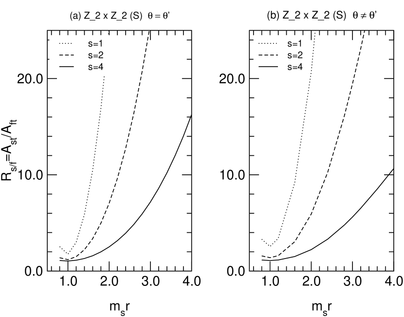
Figure 7: Plots as a function of the radius, $m_{s}r$, of the ratio of string to field theory amplitudes, ${\cal R}_{s/f}$, for the $Z_{2}\times Z_{2}$ orbifold supersymmetric $SU(5)$ gauge unified model using the subtraction regularization prescription. We show results in panel $(a)$ for the case involving equal brane intersection angles, $\theta^{I}=\theta^{{}^{\prime}I}$, and in panel $(b)$ for that involving unequal angles, $\theta^{I}\neq\theta^{{}^{\prime}I}$. The solution is described by wrapping numbers, $n_{a}=(1,1,1),\ n_{b}=(0,1,0),\ m_{a}=(1,-1,{1\over 2}),\ m_{b}=(1,0,-1)$, and angle parameters, $\pi\alpha^{I}\equiv\arctan(\tilde{m}_{a}^{I}U_{2}^{I}/n_{a}^{I})$, set at the values, $\alpha_{2}={1\over 3},\ \alpha_{1}={1\over 5},\ \alpha_{3}=(\alpha_{2}-\alpha_{1})={2\over 15}$, yielding the intersection angles, $\theta^{I}=\theta^{I}_{aa^{\prime}_{1}}=(3/5,2/3,11/15)$ and $\theta^{{}^{\prime}I}=\theta^{I}_{a_{1}b}=(3/10,1/3,11/30)$, for the modes, $10$ and $\overline{5}$, after transformation to the interval $[0,1]$.

The numerical results for the ratio of string to field theory amplitudes in the subtraction regularization procedure are displayed in Figure 7. The panels $(a)$ and $(b)$ refer to the equal and unequal intersection brane angle cases, associated to the nucleon decay amplitudes in the configurations $10\cdot 10^{\dagger}\cdot 10\cdot 10^{\dagger}$ and $10\cdot\bar{5}\cdot 10^{\dagger}\cdot\bar{5}^{\dagger}$. The dependence on the compactification radius is shown for a discrete set of values of $M_{X}$ at a fixed value of the free complex structure moduli, $\chi_{I}$, determined by the choice of $\alpha_{1},\ \alpha_{2}.$ The results are very similar to those found previously for the $Z_{3}$ orbifold. We thus conclude, in conformity with our previous conclusion from the study of $x$-integrals, that no essential difference arise for the ratio in the supersymmetric models. However, to be more conclusive in the case of the dimension ${\cal D}=5$ amplitudes, one should improve the quantitative understanding of the correlators involving excited coordinate twist fields.

We have used so far the information bearing only on the unified model by assuming a schematic representation of the gauge symmetry breaking. A fully consistent calculation of the four point baryon number violating processes requires specifying the brane setup at low energies. Explicit realizations of the deformed vacua with displaced brane stacks have been discussed in Ref. Cvetic:2001nr . The brane displacement regularization is explicitly realized by splitting some $D6$-brane stack into separated quark and lepton substacks. One can then adequately suppress the baryon number violating couplings of ${\cal D}=6,\ 5$ by increasing the distance between the substacks. We consider here the three family extended Standard Model defined in Tables $IV$ and $V$ of Ref. Cvetic:2001nr with the setup of six brane stacks, $8D6_{a_{1}},\ 8D6_{c_{1}},\ 4D6_{b_{1}},\ 2D6_{b_{2}},\ 2D6_{a_{2}},\ 4D6_{c_{2}}$, yielding the gauge group, $USp(8)_{a_{1}}\times USp(2)_{a_{2}}\times U(2)_{b_{1}}\times USp(2)_{b_{2}}\times U(4)_{c_{1}}\times USp(4)_{c_{2}}$. The brane stack splitting, $8D6_{c_{1}}=6D6_{c_{1q}}+2D6_{c_{1l}}$, resulting in $U(4)_{c_{1q}}\to U(3)_{c_{1q}}\times U(1)_{c_{1l}}$, is used to suppress the baryon number violating processes. With the first gauge factor broken as, $USp(8)_{a_{1}}\to U(1)_{8}\times U(1)_{8^{\prime}}$, the hypercharge is embedded in the linear combination, $Y={Q_{c_{1q}}\over 6}-{Q_{c_{1l}}\over 2}+{Q_{8}+Q_{8^{\prime}}\over 2}.$ The open string sector assignment for the quarks and leptons, $q\sim(b_{1},c_{1q})+(b_{1},c^{\prime}_{1q}),\ u^{c}\sim(a_{1},c_{1q}),\ d^{c}\sim(c_{1q},a_{1}),\ l\sim(c^{\prime}_{1l},b_{1})+(c_{1l},b_{1}),\ e^{c}\sim(c_{1l},a_{1})$, allows to identify the configurations of open string modes which contribute to the relevant ${\cal D}=6$ and $5$ dangerous operators,

$$\bullet\ O_{e_{L}^{c}}\sim ue^{c\dagger}u^{c\dagger}d\sim(b^{\prime}_{1},c_{1q}^{\prime})(c^{\prime}_{1l},a^{\prime}_{1})(a^{\prime}_{1},c^{\prime}_{1q})(c^{\prime}_{1q},b^{\prime}_{1}),$$ (V.14)

$$O_{e_{R}^{c}}\sim ueu^{c\dagger}d^{c\dagger}\sim(c_{1q},b^{\prime}_{1})(b^{\prime}_{1},c_{1l})(c_{1q},a_{1})(a_{1},c_{1q}),$$ (V.15)

$$\bullet\ qqql\sim ud\tilde{u}\tilde{e}\sim(b_{1},c^{\prime}_{1q})(b_{1},c_{1q})(b_{1},c^{\prime}_{1q})(c^{\prime}_{1l},b_{1}),$$ (V.16)

$$(u^{c}e^{c}\tilde{u}^{c}\tilde{d}^{c})\sim(a_{1},c_{1q})(c_{1l},a_{1})(a_{1},c_{1q})(c_{1q},a_{1}).$$ (V.17)

The above brane embeddings of the disk boundary show that while the non-supersymmetric operators, $O_{e_{L}^{c}}$ and $O_{e_{R}^{c}}$, and the supersymmetric operator, $(u^{c}e^{c}\tilde{u}^{c}\tilde{d}^{c})$, are allowed, the supersymmetric operator, $qqql$, is disallowed. Since the one-loop dressing of the operator $u^{c}e^{c}\tilde{u}^{c}\tilde{d}^{c}$ involves the exchange of electroweak higgsinos, one concludes that the nucleon decay from ${\cal D}=5$ operators should be adequately suppressed in the present model.

VI Discussion and conclusions

We have studied in this work the nucleon decay processes in semi-realistic string models of gauge unification. Our aim was to assess the stringy enhancement effect caused in the M-theory and type $II$ string theory models by the localization of matter modes in the internal space manifold. The effect has maximal strength in the large radius limit. In accounting for the effect, the reduced power dependence of the string amplitude on the unified gauge coupling constant, ${\cal A}\propto\alpha_{X}^{2/3}$, appears as a secondary manifestation in comparison to the strong peaking of the $x$-integral at the end point regions. The leading contributions from these end point regions arise from the towers of momentum modes propagating along the internal space directions wrapped by the branes.

The localization of open string modes at brane intersection points is formally analogous with that of closed string twisted modes at the orbifold fixed points. On practical grounds, an important difference is that while the distance between intersection points may be very small relative to the compactification distance scales, the fixed points of orbifold groups are generically a finite distance apart. Thus, the inevitable suppression from the classical partition function factor in closed string amplitudes may be minimized in brane models provided that the distances between intersection point are small compared to the wrapped three-cycle radius.

The consistent discussion of string unified models requires introducing an infrared matching mass scale in addition to the string parameters $g_{s},\ m_{s}$ and $r$. This is identified here with the unified gauge symmetry breaking mass scale, $M_{X}$, which may stand for the open string moduli representing either the Wilson flux line or the unified brane splitting. Since we lack a fundamental understanding of how the compactification and $D$-brane processes stabilize the closed and open string moduli, we must regard $M_{c}$ and $M_{X}$ as free parameters bounded by $m_{s}$ and differing by at most a few orders of magnitude from each other and from $m_{s}$. The relative ordering of the parameters $M_{X}$ and $M_{c}$ has a crucial impact on the enhancement effect. While a definite relation between them is implied by the heavy threshold corrections to the gauge coupling constants, we lack a quantitative understanding of these effects to make a learned choice on the relative order of $M_{X}$ and $M_{c}$. Although our study of the size of $M_{X}/M_{c}$ implied by the threshold corrections is not fully conclusive, this seems to indicate that the ordering of these scales can go both ways.

Our numerical predictions confirm that some enhancement of the string amplitude may be present at finite radius. The consitency requirements select the intervals, $M_{X}/m_{s}\in[1/4\ -\ 1]$ and $m_{s}r\in[1\ -\ 4]$. We find a significant growth of the ratio with $m_{s}r$, which is maximal for coincident intersection points. For distant intersection points the suppression effect from the classical action factor limits the ratio to values of $O(1)$. If $M_{X}<M_{c}$, the smallest contribution found with lowest $M_{X}$ leads to ratios of order $2$ at coincident intersection points and order $1$ for distant intersection points. If $M_{X}>M_{c}$, the ratio attains $O(10)$. The same conclusion applies to the configurations of brane pairs with same and distinct intersection angles. Thus, the effect is not restricted to the brane setup with same intersection angles, as concluded from the study of Ref. KW03 , based on a brane setup which did not include the unequal angle configuration.

The application to the supersymmetric model using the $Z_{2}\times Z_{2}$ orbifold indicates that a similar enhancement effect may be present in the nucleon decay processes from ${\cal D}=5$ operators. No essential difference appears in supersymmetric models, as also indicated by the similar size of the $x$-integrals for the supersymmetric and non-supersymmetric configurations of intersecting angles. Our study has an indirect bearing on the nucleon decay processes described by the dimension ${\cal D}=7,\ 9,\ 10$ operators, although we have not carried out explicit calculation of the string ampliudes in these cases. We found that restrictive selection rules are set at the tree level by the $D$-brane embedding. No finite contributions to these operators are found in the $D$-brane models discussed in the present work.

In conclusion, our calculations confirm the presence of a small enhancement effect which is maximal for diagonal configurations with same intersection points, but not necessarily carrying the same group representations. No essential changes are observed upon passing to supersymmetric amplitudes associated with the dimension $5$ operators. The string amplitudes feature a rapid growth in the regimes of large and small compactification radii relative to the string length parameter in which the string and world sheet perturbation theories are invalidated. The suppression effect in the case of distant intersection points is found to be substantial. The enhancement effect is also potentially present for the six fermion or higher order processes contributing to the $\Delta B=-2$ amplitudes at tree level. However, the examination of proposed intersecting brane models kokogut02 realizing Pati-Salam or related gauge unified models indicates that this source of baryon number violating is generically suppressed because of the absence of the higher dimensional matter modes needed to contribute to VEV induced $\Delta B=-2$ operators.

Appendix A Vacuum correlator of coordinate twist fields

We review in the present appendix the calculation of four point correlators for the open string coordinate fields obeying the twisted boundary conditions appropriate to intersecting branes wrapped around three-cycles. The restriction to factorisable $T^{6}$ tori allows us to specialize the discussion to a single $T^{2}_{I}$ torus, parameterized by the pair of complexified coordinate fields, $X^{I}(z),\ \bar{X}^{I}(z)$, with the relevant part of the stress energy generator given by, $T^{I}(z)=-{2\over\alpha^{\prime}}\partial_{z}X^{I}(z)\partial_{z}\bar{X}^{I}(z)$. For notational convenience, we restrict in the sequel to a single complex plane and omit the space component indices $I$ by identifying the string coordinates as, $X=X^{I},\ \bar{X}=\bar{X}^{I}$. We are interested in the correlators involving two distinct pairs of conjugate twist fields, $\sigma_{\pm\theta^{I}}$, with opposite sign angles, $Z^{I}(z_{i})=<\sigma_{-\theta^{I}}(z_{1})\sigma_{\theta^{I}}(z_{2})\sigma_{-\theta^{{}^{\prime}I}}(z_{3})\sigma_{\theta^{{}^{\prime}I}}(z_{4})>$. The calculations will be pursued along same lines as in the conformal field theory approach developed for the twisted sectors of heterotic string orbifold models by Dixon et al., dixon87 and Bershadsky and Radul bersh87 . Our presentation closely follows the work of Bürwick et al., burwick .

A.0.1 Quantum partition function

The energy source approach dixon87 exploits the observation that the world sheet stress energy tensor acquires a non vanishing VEV in the twisted sector vacuum created by the primary twist fields. One is thus motivated to consider the five point correlator, $Z_{T}(z;z_{i})={<T(z)\sigma_{-\theta}(z_{1})\sigma_{\theta}(z_{2})\sigma_{-\theta^{\prime}}(z_{3})\sigma_{\theta^{\prime}}(z_{4})>\over<\sigma_{-\theta}(z_{1})\sigma_{\theta}(z_{2})\sigma_{-\theta^{\prime}}(z_{3})\sigma_{\theta^{\prime}}(z_{4})>}$, obtained by inserting $T(z)$, along with the two six point correlators involving the insertion of bilocal quadratic products of the coordinate fields,

$$g(z,w;z_{i})\equiv g(z,w)={<-{2\over\alpha^{\prime}}\partial_{z}X(z)\partial_{w}\bar{X}(w)\sigma_{-\theta}(z_{1})\sigma_{\theta}(z_{2})\sigma_{-\theta^{\prime}}(z_{3})\sigma_{\theta^{\prime}}(z_{4})>\over<\sigma_{-\theta}(z_{1})\sigma_{\theta}(z_{2})\sigma_{-\theta^{\prime}}(z_{3})\sigma_{\theta^{\prime}}(z_{4})>},$$ (A.1)

$$h(\bar{z},w;z_{i})\equiv h(\bar{z},w)={<-{2\over\alpha^{\prime}}\partial_{\bar{z}}X(\bar{z})\partial_{w}\bar{X}(w)\sigma_{-\theta}(z_{1})\sigma_{\theta}(z_{2})\sigma_{-\theta^{\prime}}(z_{3})\sigma_{\theta^{\prime}}(z_{4})\over<\sigma_{-\theta}(z_{1})\sigma_{\theta}(z_{2})\sigma_{-\theta^{\prime}}(z_{3})\sigma_{\theta^{\prime}}(z_{4})>}.$$ (A.2)

The correlators $g(z,w),\ h(\bar{z},w)$ are meromorphic functions of $z,\ \bar{z}$ and $w$, whose singularities are fully determined by the operator product expansion of the primary twist fields, as given in Eqs. (II.31). The fact that the short distance expansion in the limit $z\to w$ of $g(z,w)$ exhibits a double pole term, allows one to relate this function to the correlator $Z_{T}(z;z_{i})$ as

$$-{2\over\alpha^{\prime}}\partial X(z)\partial\bar{X}(w)={1\over(z-w)^{2}}+T(z)+\cdots\ \Longrightarrow\ g(z,w)={1\over(z-w)^{2}}+Z_{T}(z;z_{i})+\cdots,$$ (A.3)

where the dots represent the higher order terms in the expansion in powers of $(z-w)$. Since no singularities are present in the limit $\bar{z}\to w$, one concludes that the bilocal correlator $h(\bar{z},w)$ has no pole terms and so must tend to a constant in this limit. Writing the short distance expansion of $Z_{T}(z;z_{i})$ in the limit $z\to z_{I},\$ for fixed index $I$, with the help of the familiar operator product expansion

$$T(z)\sigma_{\theta}(z_{I})={h(\sigma_{\theta})\sigma_{\theta}(z)\over(z-z_{I})^{2}}+{\partial_{z_{I}}\sigma_{\theta}(z_{I})\over(z-z_{I})},\ [h(\sigma_{\theta})={1\over 2}\theta(1-\theta)]$$ (A.4)

yields the differential equation relating the correlators $Z(z_{i})$ and $Z_{T}(z;z_{i})$

$${\partial\over\partial z_{I}}\ln Z(z_{i})=(z-z_{I})Z_{T}(z;z_{i})-{h(\sigma_{\theta})\over z-z_{I}}.$$ (A.5)

The holomorphy properties of the functions $g(z,w)$ and $h(\bar{z},w)$, as the variables $z,\ \bar{z}$ and $w$ approach the insertion points $z_{i}$, allows one to write the following general representations for these functions,

$$g(z,w)=\omega_{\theta,\theta^{\prime}}(z)\omega_{1-\theta,1-\theta^{\prime}}(w)\bigg{[}{P(z,w)\over(z-w)^{2}}+A(z_{i})\bigg{]},\ h(\bar{z},w)=\bar{\omega}_{1-\theta,1-\theta^{\prime}}(\bar{z})\omega_{1-\theta,1-\theta^{\prime}}(w)B(z_{i}),$$ (A.6)

(A.7)

$$\bigg{[}\omega_{\theta,\theta^{\prime}}(z)=(z-z_{1})^{-\theta}(z-z_{2})^{\theta-1}(z-z_{3})^{-\theta^{\prime}}(z-z_{4})^{\theta^{\prime}-1},$$ (A.8)

$$\omega_{1-\theta,1-\theta^{\prime}}(w)=(w-z_{1})^{\theta-1}(w-z_{2})^{-\theta}(w-z_{3})^{\theta^{\prime}-1}(w-z_{4})^{-\theta^{\prime}},$$ (A.9)

$$\bar{\omega}_{1-\theta,1-\theta^{\prime}}(\bar{z})=(\bar{z}-z_{1})^{\theta-1}(\bar{z}-z_{2})^{-\theta}(\bar{z}-z_{3})^{\theta^{\prime}-1}(\bar{z}-z_{4})^{-\theta^{\prime}},$$ (A.10)

$$P(z,w)=\sum_{i,j=0}^{2}\alpha_{ij}w^{i}z^{j}=\alpha_{00}+\alpha_{01}z+\alpha_{10}w+\alpha_{20}w^{2}$$ (A.11)

$$+(\alpha_{11}w+\alpha_{21}w^{2})z+(\alpha_{02}+\alpha_{12}w+\alpha_{22}w^{2})z^{2}\bigg{]}$$ (A.12)

where the coefficients $A(z_{i}),\ B(z_{i})$ (to be determined in the sequel via the global monodromy conditions) and the coefficients $\alpha_{jk}$ of the second order polynomial $P(z,w)$ are functions of the insertion points $z_{i}$. The polynomial $P(z,w)$ is determined by the requirement that one reproduces the pole structure, $g(z,w)\to(z-w)^{-2}$, in the limit $z\to w$. Expanding the various factors of $g(z,w)$ in powers of $(w-z)$ leads to the two sets of relations:

$$\bullet\ P(z,z)=[\omega_{\theta,\theta^{\prime}}(z)\omega_{1-\theta,1-\theta^{\prime}}(z)]^{-1}=\prod_{i}(z-z_{i})$$ (A.13)

$$\Longrightarrow\ \alpha_{00}=z_{1}z_{2}z_{3}z_{4},\ \alpha_{10}+\alpha_{01}=-(z_{2}z_{3}z_{4}+z_{3}z_{4}z_{1}+z_{4}z_{1}z_{2}+z_{1}z_{2}z_{3}),$$ (A.14)

$$\alpha_{11}+\alpha_{02}+\alpha_{20}=z_{3}z_{4}+z_{4}z_{1}+z_{1}z_{2}+z_{2}z_{3},\ \alpha_{21}+\alpha_{12}=-(z_{1}+z_{2}+z_{3}+z_{4}),\ \alpha_{22}=1,$$ (A.15)

$$\bullet\ {P^{\prime}(z,z)\over P(z,z)}=-{\omega^{\prime}_{1-\theta,1-\theta^{\prime}}(z)\over\omega_{1-\theta,1-\theta^{\prime}}(z)}=\bigg{[}{\theta-1\over z-z_{1}}+{\theta^{\prime}-1\over z-z_{3}}-{\theta\over z-z_{2}}-{\theta^{\prime}\over z-z_{4}}\bigg{]}$$ (A.16)

$$\Longrightarrow\ \alpha_{10}=\theta z_{3}z_{4}(z_{2}-z_{1})+\theta^{\prime}z_{1}z_{2}(z_{4}-z_{3})-z_{2}z_{4}(z_{3}+z_{1}),$$ (A.17)

$$2\alpha_{21}+\alpha_{12}=-[\theta(z_{1}-z_{2})+\theta^{\prime}(z_{3}-z_{4})+2(z_{2}+z_{4})+z_{1}+z_{3}],$$ (A.18)

$$\alpha_{11}+2\alpha_{20}=-[(\theta-1)(z_{3}z_{4}+z_{2}z_{4}+z_{2}z_{3})+(\theta^{\prime}-1)(z_{2}z_{4}+z_{1}z_{4}+z_{1}z_{2})$$ (A.19)

$$-\theta(z_{3}z_{4}+z_{1}z_{4}+z_{1}z_{3})-\theta^{\prime}(z_{2}z_{3}+z_{1}z_{3}+z_{1}z_{2})],$$ (A.20)

allowing to express the solution for the $T(z)$-inserted correlator as

$$Z_{T}(z;z_{i})=\omega_{\theta,\theta^{\prime}}(z)\omega^{\prime}_{1-\theta,1-\theta^{\prime}}(z)P^{\prime}(z,z)+{1\over 2}\omega_{\theta,\theta^{\prime}}(z)\omega^{\prime\prime}_{1-\theta,1-\theta^{\prime}}(z)P(z,z)$$ (A.21)

$$+\omega_{\theta,\theta^{\prime}}(z)\omega_{1-\theta,1-\theta^{\prime}}(z)\bigg{(}A(z_{i})+{1\over 2}P^{\prime\prime}(z,z)\bigg{)}$$ (A.22)

$$=-\omega_{\theta,\theta^{\prime}}(z)\omega^{\prime}_{1-\theta,1-\theta^{\prime}}(z)P^{2}(z,z)+{1\over 2}\omega_{\theta,\theta^{\prime}}(z)\omega^{\prime\prime}_{1-\theta,1-\theta^{\prime}}(z)P(z,z)$$ (A.23)

$$+(A(z_{i})+\alpha_{20}+\alpha_{21}z+z^{2})P(z,z),$$ (A.24)

with the primes standing for the derivative $\partial_{w}$, namely, $P^{\prime}(z,w)=\partial_{w}P(z,w),\ P^{\prime\prime}(z,w)=\partial^{2}_{w}P(z,w)$. The equations for the coefficients, $\alpha_{12},\ \alpha_{21}$, are independently solved, with the solutions given by, $\alpha_{12}=(\theta-1)z_{1}-(\theta+1)z_{2}+(\theta^{\prime}-1)z_{3}-(\theta^{\prime}+1)z_{4},\ \alpha_{21}=-[\theta z_{1}+\theta^{\prime}z_{3}+(1-\theta)z_{2}+(1-\theta^{\prime})z_{4}].$ The condition on the double pole term gives eight linear equations for the nine coefficients, $\alpha_{ij}$. However, since the coefficient $\alpha_{20}$ can always be absorbed inside the function $A(z_{i})$, this coefficient remains arbitrary as long as $A(z_{i})$ is unspecified. We make the convenient choice burwick , $\alpha_{20}={1\over 2}[(\theta+\theta^{\prime})(z_{1}z_{3}-z_{2}z_{4})+(\theta-\theta^{\prime})(z_{1}z_{4}-z_{2}z_{3})+2z_{2}z_{4}]$, which then fully determines $P(z,w)$. Evaluating the function $g(z,w)$ by taking first the limit, $w\to\infty$, and next the limit, $z\to z_{2}$, leads to the differential equation for the correlator of interest

$${\partial\over\partial z_{2}}\ln Z(z_{i})={\theta-\theta^{\prime}\over 2}{z_{34}\over z_{23}z_{24}}+{\theta(1-\theta)\over z_{12}}+\theta(1-\theta^{\prime})\bigg{(}{1\over z_{32}}+{1\over z_{24}}\bigg{)}+{A(z_{i})\over z_{21}z_{23}z_{24}},$$ (A.25)

where we use the notation, $z_{ij}\equiv z_{i}-z_{j}$, and have set $z_{J}=z_{2}$. Similar equations apply by letting $z$ approach the other insertion points. Thanks to the invariance under the $SL(2,R)$ subgroup of the conformal group, one can arbitrarily fix three insertion points. With the choice of insertion points along the real axis boundary, $z_{1}=x_{1}=0,z_{3}=x_{3}=1,z_{4}=x_{4}=X\to\infty$, leaving the single real variable, $z_{2}=x_{2}=x\in[-\infty,\infty]$, one can reconstruct the full dependence by noting that the Möbius group invariant functions of four variables in $C$ can only depend on the harmonic ratio variable, $x={z_{21}z_{34}\over z_{24}z_{31}}$. (Note that $(1-x)={z_{23}z_{41}\over z_{24}z_{31}}$.) The so far unspecified coefficients of the polynomial $P(z,w)$ are now given by the simpler formulas, $\alpha_{20}=X[{1\over 2}(\theta-\theta^{\prime})+x(1-{\theta+\theta^{\prime}\over 2})],\ \alpha_{11}=X(-\theta+\theta^{\prime}+1+x\theta^{\prime}),\ \alpha_{02}={X\over 2}[-x+(\theta-\theta^{\prime})(1-x)].$ It is convenient to absorb the known dependence on the variable $X$ by considering the reduced correlator and coefficients identified by hats, $Z(z_{i})=\hat{Z}(x)(x-X)^{\theta(1-\theta^{\prime})},\ A(z_{i})=(x-X)\hat{A}(x),\ B(z_{i})=(x-X)\hat{B}(x)$. The differential equation for the reduced correlator reads then as,

$${\partial\over\partial x}\ln\hat{Z}(x)=-{\theta-\theta^{\prime}\over 2(1-x)}+{\theta(1-\theta^{\prime})\over(1-x)}-{\theta(1-\theta)\over x}-{\hat{A}(x)\over x(1-x)}.$$ (A.26)

To proceed further at this point, one must separate out the zero mode part of the coordinate field, associated with the classical zero modes, from its quantum or oscillator part. The additive splitting, $X(z)=X_{cl}(z)+X_{qu}(z)$, produces the multiplicative splitting of the correlator into classical and quantum factors, $\hat{Z}(x)=Z_{qu}(x)Z_{cl}(x),\ [Z_{cl}(x)=\sum_{cl}e^{-S_{cl}(x)}]$ where the classical factor represents the contribution from the world sheet instantons and anti-instantons, defined as the Euclidean space coordinate field solutions of the world sheet equations of motion, $\partial_{z}X_{cl}(z)=0,\ \partial_{\bar{z}}X_{cl}(\bar{z})=0$. The general solutions with the appropriate singularities at the insertion points, $z_{i}$, are described in terms of the meromorphic functions introduced earlier as, $\partial_{z}X_{cl}(z)=b\omega_{\theta,\theta^{\prime}}(z),\ \partial_{\bar{z}}X_{cl}(\bar{z})=c\bar{\omega}_{1-\theta,1-\theta^{\prime}}(\bar{z})$, where the complex constants $b,\ c$ represent free continuous parameters.

We postpone the discussion of the classical partition function until the next subsection, and continue with the study of the quantum factor. The coefficients $A(z_{i}),\ B(z_{i})$ are determined by imposing the global boundary conditions requiring that the quantum components of coordinate fields, unlike the classical ones, are single valued functions on the cut complex plane $C$. For definiteness, we consider the four point amplitude with the configuration of open string sectors, $<V_{-\theta,{(D,A)}}(x_{1})V_{\theta,{(A,B)}}(x_{2})V_{-\theta^{\prime},{(B,C)}}(x_{3})V_{\theta^{\prime},{(C,D)}}(x_{4})>$, setting the boundary along the real axis of $C_{+}$, with $z_{i}=x_{i}.$ The embedding in $T^{2}_{I}$ is described by the four-polygon displayed in Figure 8, with vertices and edges given by the images of insertion points, $x_{1},\cdots,x_{4}$, and arc segments, $S_{\alpha}=(x_{1},x_{2}),\ (x_{2},x_{3}),\ (x_{3},x_{4}),\ (x_{4},x_{1})$, along the disk boundary. On the four segments covering the periodic real axis, $[A,B,C,D]=[(x_{1},x_{2}),\ (x_{2},x_{3}),\ (x_{3},x_{4}),\ (x_{4},x_{1})]$, the complex coordinate fields obey the relations,

$$e^{-i\phi^{I}_{S}}\partial X^{I}(z)-e^{i\phi^{I}_{S}}\bar{\partial}\bar{X}^{I}(\bar{z})=0,\ e^{-i\phi^{I}_{S}}\bar{\partial}X^{I}(\bar{z})-e^{i\phi^{I}}\partial\bar{X}^{I}(z)=0,\ [S=A,B,C,D]$$ (A.27)

with the interbrane angles assigned in the various intervals as, $\phi_{D}=0,\ \phi_{A}=\phi=\pi\theta,\ \phi_{B}=0,\ \phi_{C}=\phi^{\prime}=\pi\theta^{\prime}.$ Since the vector space of contours is of dimension $2$, it suffices to consider the integrated form of the boundary conditions for two independent contours. We choose the contours $C_{1},\ C_{2}$ along the branes $A$ and $B$, with angles $\phi_{A}=\pi\theta$ and $\phi_{B}=0$. To establish contact with the formalism used for closed strings, it is convenient to consider instead the associated closed contours (or cycles) surrounding the intervals for the open contours, $C_{i}\in C_{+}$. The cycles ${\cal C}_{i}\in C$ are defined by adding to the contours $C_{i}$ their reflected image $C^{\prime}_{i}$ with respect to the real axis boundary, ${\cal C}_{i}=C_{i}-C^{\prime}_{i},\ [i=1,4]$. This definition of the fields dispenses one from the need to define the analytic continuation of fields on the Riemann sheets of the cut plane $C$. We now consider the contour integrals on $C_{i}$ for the sum of the two boundary conditions in Eqs.(A.27), and reshuffle the two pairs of terms so as to express these as cycle integrals on the basis of independent cycles, ${\cal C}_{i}$ by using the transformation under the reflection, $\partial X\to e^{2i\phi_{S}}\partial\bar{X}$ and $\bar{\partial}X\to e^{2i\phi_{S}}\bar{\partial}\bar{X}$. The resulting integrated boundary conditions on the coordinate fields

$$0=\int_{C_{i}}[(\partial X-e^{2i\phi_{S}}\bar{\partial}\bar{X})+(\bar{\partial}X-e^{2i\phi_{S}}\partial\bar{X})]=\int_{C_{i}-C^{\prime}_{i}}(\partial X+\bar{\partial}X)=\int_{{\cal C}_{i}}(\partial X+\bar{\partial}X),$$ (A.28)

are then used to express the trivial monodromy conditions on the quantum component of the six-point correlators, $0=\int_{{\cal C}_{i}}dzg(z,w)+\int_{{\cal C}_{i}}d\bar{z}h(\bar{z},w).$ This is our first encounter with the mixed type correlator, $h(\bar{z},w)$. The two integrals along the contours $C_{1},\ C_{2}$ give the relations needed to determine the two unknown coefficients, $A(z_{i}),\ B(z_{i})$. We note that $\int_{{\cal C}_{1}}\sim\int_{0}^{x},\ \int_{{\cal C}_{2}}\sim\int_{x}^{1}.$ Substituting Eqs. (A.12) for $g(z,w),\ h(\bar{z},w)$ into the integrals over the cycles ${\cal C}_{1},\ {\cal C}_{2}$, gives the pair of equations for $i=(1,2)$,

$$\hat{A}(x)\int_{{\cal C}_{i}}dz\omega_{\theta,\theta^{\prime}}(z)+\hat{B}(x)\int_{{\cal C}_{i}}d\bar{z}\bar{\omega}_{1-\theta,1-\theta^{\prime}}(\bar{z})$$ (A.30)

$$=-x{(\theta-\theta^{\prime})\over 2}\int_{{\cal C}_{i}}dz\omega_{\theta,\theta^{\prime}}(z)-(1-\theta^{\prime})\int_{{\cal C}_{i}}dz(z-x)\omega_{\theta,\theta^{\prime}}(z)=x(1-x)\partial_{x}\int_{{\cal C}_{i}}dz\omega_{\theta,\theta^{\prime}}(z),$$ (A.31)

where the last step is deduced by integration by parts. The resulting two linear equations for the coefficients $\hat{A}(x),\ \hat{B}(x)$, obtained with ${\cal C}_{1},\ {\cal C}_{2}$, can be expressed by the matrix equation,

$$\pmatrix{\int_{{\cal C}_{1}}dz\omega_{\theta,\theta^{\prime}}(z)&\int_{{\cal C}_{1}}d\bar{z}\bar{\omega}_{1-\theta,1-\theta^{\prime}}(\bar{z})\cr\int_{{\cal C}_{2}}dz\omega_{\theta,\theta^{\prime}}(z)&\int_{{\cal C}_{2}}d\bar{z}\bar{\omega}_{1-\theta,1-\theta^{\prime}}(\bar{z})}\pmatrix{\hat{A}(x)\cr\hat{B}(x)}=x(1-x)\partial_{x}\pmatrix{\int_{{\cal C}_{1}}dz\omega_{\theta,\theta^{\prime}}(z)\cr\int_{{\cal C}_{2}}dz\omega_{\theta,\theta^{\prime}}(z)}.$$ (A.33)

These equations are readily solved for $\hat{A}(x),\ \hat{B}(x)$, with the explicit formula for $\hat{A}(x)$ reading as

$$\hat{A}(x)=x(1-x){(\partial_{x}\int_{{\cal C}_{2}}\omega_{\theta,\theta^{\prime}})(\int_{{\cal C}_{1}}\bar{\omega}_{1-\theta,1-\theta^{\prime}})-(\partial_{x}\int_{{\cal C}_{1}}\omega_{\theta,\theta^{\prime}})(\int_{{\cal C}_{2}}\bar{\omega}_{1-\theta,1-\theta^{\prime}})\over(\int_{{\cal C}_{1}}\bar{\omega}_{1-\theta,1-\theta^{\prime}})(\int_{{\cal C}_{2}}\omega_{\theta,\theta^{\prime}})-(\int_{{\cal C}_{2}}\bar{\omega}_{1-\theta,1-\theta^{\prime}})(\int_{{\cal C}_{1}}\omega_{\theta,\theta^{\prime}})}={1\over 2}x(1-x)\partial_{x}\ln I(x),$$ (A.34)

$$[I(x)={1\over(2i\pi)^{2}}e^{i\pi(4-p)\theta-2i\pi\theta^{\prime}}[(\int_{{\cal C}_{1}}\omega_{\theta,\theta^{\prime}})(\int_{{\cal C}_{2}}\bar{\omega}_{1-\theta,1-\theta^{\prime}})-(\int_{{\cal C}_{2}}\omega_{\theta,\theta^{\prime}})(\int_{{\cal C}_{1}}\bar{\omega}_{1-\theta,1-\theta^{\prime}})]$$ (A.35)

where to simplify the notations we have omitted writing the integration measure factors $dz$ or $d\bar{z}$ in the cycle integrals. For the purpose of simplifying the final results, we have set the so far undetermined constant normalization of $I(x)$ to a conveniently chosen value depending on the parameter $p$. Explicit analytic formulas for the cycle integrals will be presented shortly. The total derivative structure of the function, $\hat{A}(x)/[x(1-x)]$, in Eq. (A.35) transforms the differential equation for $Z_{qu}(x)$ in Eq. (A.26) to the simple form, $\partial_{x}\ln(Z_{qu}(x)I^{1\over 2}(x))=-\theta(1-\theta)/x+[\theta(1-\theta^{\prime})+\theta^{\prime}(1-\theta)]/[2(1-x)]$, which is readily solved to give the final form of the quantum partition function,

$$Z_{qu}^{I}(x)=C_{\sigma}x^{-\theta^{I}(1-\theta^{I})}(1-x)^{-{1\over 2}\theta^{{}^{\prime}I}(1-\theta^{I})-{1\over 2}\theta^{I}(1-\theta^{{}^{\prime}I})}I^{-{1\over 2}}(x),$$ (A.36)

where we have reinstated the complex plane label, $I$. The constant $C_{\sigma}$ can be determined by making use of the pole factorization of the correlator. Note that we have corrected a confusing misprint in Eqs.(3.21) and (3.37) of the work by Bürwick et al., burwick . These would have given a wrong dependence of the exponent of $(1-x)$, lacking the symmetry under $\theta\leftrightarrow\theta^{\prime}$, which our above result exhibits explicitly. The integrals over the two independent cycles have the following analytic forms

$$\int_{{\cal C}_{1}}dz\omega_{\theta,\theta^{\prime}}(z)=2\pi ie^{2\pi i({\theta^{\prime}\over 2}-\theta)}G_{2}(x),$$ (A.37)

$$\int_{{\cal C}_{2}}dz\omega_{\theta,\theta^{\prime}}(z)=2i\sin(\pi p\theta)(1-x)^{\theta-\theta^{\prime}}e^{i\pi[(p-2)\theta+\theta^{\prime}]}B_{1}H_{1}(1-x),$$ (A.38)

$$\int_{{\cal C}_{1}}d\bar{z}\bar{\omega}_{1-\theta,1-\theta^{\prime}}(\bar{z})=2\pi ie^{2\pi i({\theta^{\prime}\over 2}-\theta)}\bar{G}_{1}(x),$$ (A.39)

$$\int_{{\cal C}_{2}}d\bar{z}\bar{\omega}_{1-\theta,1-\theta^{\prime}}(\bar{z})=-2i\sin(\pi p\theta)(1-x)^{\theta^{\prime}-\theta}e^{i\pi[(p-2)\theta+\theta^{\prime}]}B_{2}\bar{H}_{2}(1-x),$$ (A.40)

$$\ \Longrightarrow\ I(x)={\sin(\pi p\theta)\over\pi}(B_{2}\bar{G}_{1}H_{2}+B_{1}\bar{G}_{2}H_{1}),$$ (A.41)

$$\bigg{[}B_{1}=B(\theta,1-\theta^{\prime})\equiv{\Gamma(\theta)\Gamma(1-\theta^{\prime})\over\Gamma(1+\theta-\theta^{\prime})},\ B_{2}=B(\theta^{\prime},1-\theta)\equiv{\Gamma(1-\theta)\Gamma(\theta^{\prime})\over\Gamma(1-\theta+\theta^{\prime})},$$ (A.42)

$$G_{1}(x)=F(\theta,1-\theta^{\prime};1;x),\ G_{2}(x)=F(1-\theta,\theta^{\prime};1;x),$$ (A.43)

$$H_{1}(x)=F(\theta,1-\theta^{\prime};1+\theta-\theta^{\prime};x),\ H_{2}(x)=F(1-\theta,\theta^{\prime};1-\theta+\theta^{\prime};x),$$ (A.44)

$$F(a,b;c;x)={\Gamma(c)\over\Gamma(b)\Gamma(c-b)}\int_{0}^{1}dtt^{b-1}(1-t)^{c-b-1}(1-xt)^{-a}\bigg{]}$$ (A.45)

where $B(a,b)$ and $\Gamma(z)$ designate the Euler Beta and Gamma functions and $F(a,b;c;z)$ the Riemann Hypergeometric function. Although we have kept track in the above formulas of the complex conjugate functions, signalled by the bar symbol, this distinction is not relevant here to the extent that the restriction of the various functions to the real axis are real.

A.0.2 Classical partition function

We now return to the calculation of the classical action factor, $Z_{cl}=\sum_{cl}e^{-S_{cl}}$, where the summation extends over the non-trivial monodromies around the cycles ${\cal C}_{i}$ of the coordinate field classical solutions, $X_{cl}(z,\bar{z})$. For orientation, we recall that in the simpler case of $S^{1}$ circle compactification, the classical summation extends over the 1-d lattice of solutions with winding numbers, $\sqrt{2}\Delta_{\cal C}X=\sqrt{2}\int_{S^{1}}dX=2\pi v,\ [v\in Z]$. In the $T^{2}_{I}$ torus case, the monodromies of the coordinate $X^{I}$ around the cycles, ${\cal C}_{1},\ {\cal C}_{2}$, belong to the 2-d grand lattice generated by the cycles along the $D6_{A}/D6_{B}-$branes, images of ${\cal C}_{1},\ {\cal C}_{2}$, possibly shifted by the non-vanishing distance between distant intersection points. Denoting the intersection points along the branes $D6_{A}$ and $D6_{B}$ by $f_{1}^{A},\ f_{2}^{A}$ and $f_{2}^{B},\ f_{3}^{B}$, in correspondence with the images of the insertion points $x_{1},\ x_{2}$ and $x_{3}$, one can express the non-trivial monodromy conditions on the classical components of coordinate fields, $\Delta_{{\cal C}_{i}}X^{I}\equiv\int_{{\cal C}_{1}}(dz\partial X^{I}+d\bar{z}\bar{\partial}X^{I})$, for the cycle basis ${\cal C}_{1,2}$ mapped to the $D$-branes $A,\ B$, in terms of the 2-d lattice generated by the $D$-brane pair, $L_{A},\ L_{B}$, as

$$\sqrt{2}\Delta_{{\cal C}_{1}}X^{I}\equiv 2\pi v_{A}=2\pi(1-e^{2i\pi\theta})(f^{A}_{1}-f^{A}_{2}+p_{A}L_{A}),$$ (A.46)

$$\sqrt{2}\Delta_{{\cal C}_{2}}X^{I}\equiv 2\pi v_{B}=2\pi(1-e^{2i\pi\theta})(f^{B}_{2}-f^{B}_{3}+p_{B}L_{B}),$$ (A.47)

where we have assumed, for simplicity, the brane lattice to be generated by the integers $p_{A},\ p_{B}\in Z.$ The relation $\Delta_{{\cal C}_{i}}X=\Delta_{C_{i}-C^{\prime}_{i}}X=(1-e^{2i\pi\theta})X,\ [i=1,2]$ follows from the $2\pi\theta$ rotation of coordinates along the reflected contours. If we had used the open contours in the upper complex plane, $C_{+}$, as in the presentation by Cvetic and Papadimitriou Cvetic:2003ch , similar formulas to the above would hold, but without the angle dependent factors, $(1-e^{2i\pi\theta})$. To relate the integer quantized winding numbers $p_{A},\ p_{B}$ with the coefficients $b,\ c$ in the instanton and anti-instanton solutions, it is convenient to introduce the 2-d bases of holomorphic and antiholomorphic solutions, $X^{(i)},\ [i=1,2]$ defined by

$$\sqrt{2}\partial X^{(1)}(z)=b_{1}\omega_{\theta,\theta^{\prime}}(z),\ \sqrt{2}\partial X^{(2)}(z)=b_{2}\omega_{\theta,\theta^{\prime}}(z),$$ (A.48)

$$\sqrt{2}\bar{\partial}X^{(1)}(\bar{z})=c_{1}\bar{\omega}_{1-\theta,1-\theta^{\prime}}(\bar{z}),\ \sqrt{2}\bar{\partial}X^{(2)}(\bar{z})=c_{2}\bar{\omega}_{1-\theta,1-\theta^{\prime}}(\bar{z}).$$ (A.49)

The condition that the $X^{(i)}$ constitute the dual basis to the basis of cycles, ${\cal C}_{i}$, is expressed by the orthonormalization relations,

$$2\pi\delta_{ij}=\sqrt{2}\Delta_{{\cal C}_{i}}X^{(j)}=\sqrt{2}\int_{{\cal C}_{i}}dz\partial X^{(j)}(z)+\sqrt{2}\int_{{\cal C}_{i}}d\bar{z}\bar{\partial}X^{(j)}(\bar{z}),\ [i,j=1,2].$$ (A.50)

Expressing the general classical solutions as linear superpositions of the two solutions in Eqs. (A.49),

$$\sqrt{2}\partial X\equiv b\omega_{\theta,\theta^{\prime}}(z)=\sqrt{2}(v_{A}\partial X^{(1)}+v_{B}\partial X^{(2)})\equiv(b_{1}v_{A}+b_{2}v_{B})\omega_{\theta,\theta^{\prime}}(z)\$$ (A.51)

$$\sqrt{2}\bar{\partial}X\equiv c\bar{\omega}_{1-\theta,1-\theta^{\prime}}(\bar{z})=\sqrt{2}(v_{A}\bar{\partial}X^{(1)}+v_{B}\bar{\partial}X^{(2)})\equiv(c_{1}v_{A}+c_{2}v_{B})\bar{\omega}_{1-\theta,1-\theta^{\prime}}(\bar{z}),$$ (A.52)

allows identifying the coefficients $b,\ c$ as, $b=b_{1}v_{A}+b_{2}v_{B}$ and $c=c_{1}v_{A}+c_{2}v_{B}$, where $v_{A},\ v_{B}$ are the lattice vectors defined in Eqs.(A.47). The four conditions, $2\pi=\sqrt{2}\Delta_{{\cal C}_{1,2}}X^{(1),(2)},\ 0=\sqrt{2}\Delta_{{\cal C}_{1,2}}X^{(2),(1)},$ may now be used to obtain four linear equations for the four constant coefficients $b_{i},\ c_{i}$, whose solution is given by

$$b_{1}={2\pi\over J}\int_{{\cal C}_{2}}d\bar{z}\bar{\omega}_{1-\theta,1-\theta^{\prime}}(\bar{z}),\ b_{2}=-{2\pi\over J}\int_{{\cal C}_{1}}d\bar{z}\bar{\omega}_{1-\theta,1-\theta^{\prime}}(\bar{z}),$$ (A.53)

$$c_{1}=-{2\pi\over J}\int_{{\cal C}_{2}}dz\omega_{\theta,\theta^{\prime}}(z),\ c_{2}={2\pi\over J}\int_{{\cal C}_{1}}dz\omega_{\theta,\theta^{\prime}}(z),$$ (A.54)

$$[J=(\int_{{\cal C}_{1}}\omega_{\theta,\theta^{\prime}}(z))(\int_{{\cal C}_{2}}\bar{\omega}_{1-\theta,1-\theta^{\prime}}(\bar{z}))-(\int_{{\cal C}_{1}}\bar{\omega}_{1-\theta,1-\theta^{\prime}}(\bar{z}))(\int_{{\cal C}_{2}}\omega_{\theta,\theta^{\prime}}(z))].$$ (A.55)

The final step involves substituting the above solutions into the string classical action,

$$S_{cl}={1\over 2\pi\alpha^{\prime}}\int_{C}d^{2}z(\partial X\bar{\partial}\bar{X}+\bar{\partial}X\partial\bar{X})$$ (A.56)

$$\equiv{1\over 2\pi\alpha^{\prime}}\int_{C}d^{2}z(|\partial X|^{2}+|\bar{\partial}X|^{2}=V_{11}|v_{A}|^{2}+V_{22}|v_{B}|^{2}+2\Re(V_{12}v_{A}v_{B}^{\star}),$$ (A.57)

$$\bigg{[}4\pi V_{ii}=|b_{a}|^{2}\int_{C}d^{2}z|\omega_{\theta,\theta^{\prime}}(z)|^{2}+|c_{a}|^{2}\int_{C}d^{2}z|\omega_{1-\theta,1-\theta^{\prime}}(z)|^{2},\ [i=1,2]$$ (A.58)

$$4\pi V_{12}=b_{1}\bar{b}_{2}\int_{C}d^{2}z|\omega_{\theta,\theta^{\prime}}(z)|^{2}+c_{1}\bar{c}_{2}\int_{C}d^{2}z|\omega_{1-\theta,1-\theta^{\prime}}(z)|^{2}\bigg{]}$$ (A.59)

and evaluating the complex plane integrals for the holomorphic and antiholomorphic differentials by making use of the analytic continuation method of Kawai et al., kawai86 . Using the analytic formulas for these integrals in Eq. (A.45) along with the previously derived formulas for the coefficients, $b_{i},\ c_{i}$, in Eq. (A.55) gives the following results for the functions $V_{ij}$ determining the classical action

$$V_{11}={1\over 4I^{2}(x)}({\sin\pi p\theta\over\pi})^{2}[|B_{2}H_{2}|^{2}(2\Re(B_{1}G_{1}H_{1})-c_{\theta,\theta^{\prime}}|G_{1}|^{2})$$ (A.60)

$$+|B_{1}H_{1}|^{2}(2\Re(B_{2}G_{2}H_{2})+c_{\theta\theta^{\prime}}|G_{2}|^{2})],$$ (A.61)

$$V_{22}={1\over 4I^{2}(x)}2\Re[G_{1}G_{2}(B_{2}\bar{G}_{1}\bar{H}_{2}+B_{1}\bar{G}_{2}\bar{H}_{1})],$$ (A.62)

$$V_{12}={1\over 4I^{2}(x)}{\sin\pi p\theta\over\pi}e^{i\pi p\theta}[B_{2}G_{2}\bar{H}_{2}(2\Re(B_{1}G_{1}\bar{H}_{1})-c_{\theta\theta^{\prime}}|G_{1}|^{2})$$ (A.63)

$$-B_{1}\bar{G}_{1}H_{1}(2\Re(B_{2}G_{2}\bar{H}_{2})+c_{\theta\theta^{\prime}}|G_{2}|^{2})],$$ (A.64)

$$[c_{\theta,\theta^{\prime}}=\pi(\cot(\pi\theta)-\cot(\pi\theta^{\prime}))]$$ (A.65)

where $I(x)$ is given by the analytic formula quoted in Eq. (A.45). To obtain the classical partition factor, $Z_{cl}$, it now remains to sum over the 2-d integer lattice generated by the pairs of branes. The comparison with the classical partition function for closed strings in orbifolds in Ref. burwick , whose notations we have closely followed, indeed shows that the open string correlator is the square root truncation of the closed string correlator. With our choice of closed contours, the parameter $p$ in the definition of Eq.(A.45) for the function $I(x)$ must be set to unity, $p=1$.

A.0.3 Useful limiting formulas

To ensure that the series for the instanton sums converge at the end points $x=0,\ 1$, thus avoiding the end point singularities in the $x$-integral of string amplitudes, it is necessary to make use of the Poisson resummation formula. This is also needed for a proper identification of the particle exchange pole contributions in the field theory limit. We record below the limiting forms of some intermediate results at the end points of the interval, $x\in(0,1)$. The limiting formulas at $x\to 0$ are given by

$$F(\theta,1-\theta;1;x)\to 1,\ F(\theta,1-\theta;1;1-x)\to{\sin(\pi\theta)\over\pi}\log{\delta(\theta)\over x},$$ (A.66)

$$B_{1}H_{1}(x)\to\ln{\delta_{1}\over x},\ B_{2}H_{2}(x)\to\ln{\delta_{2}\over x},$$ (A.67)

$$V_{11}\to{1\over 4}\ln{\hat{\delta}\over x},\ V_{12}\to-e^{i\pi p\theta}{\pi^{2}(\cot(\pi\theta)-\cot(\pi\theta^{\prime}))\over 8\sin(\pi p\theta)\ln(\hat{\delta}/x)},\ V_{22}\to{\pi^{2}\over 4\sin^{2}(\pi p\theta)\ln(\hat{\delta}/x)},$$ (A.68)

$$\bigg{[}\ln\delta(\theta)=2\psi(1)-\psi(\theta)-\psi(1-\theta),\ \ln\delta_{1}(\theta,\theta^{\prime})=2\psi(1)-\psi(1-\theta^{\prime})-\psi(\theta),$$ (A.69)

$$\ln\delta_{2}(\theta,\theta^{\prime})=2\psi(1)-\psi(1-\theta)-\psi(\theta^{\prime}),\ \hat{\delta}(\theta,\theta^{\prime})=[\delta_{1}(\theta,\theta^{\prime})\delta_{2}(\theta,\theta^{\prime})]^{1\over 2},$$ (A.70)

$$\psi(1)=-\gamma,\ \psi(1-z)-\psi(z)=\pi\cot(\pi z),\ \Gamma(z)\Gamma(1-z)={\pi\over\sin(\pi z)}\bigg{]},$$ (A.71)

where $\psi(z)=\psi^{(1)}(z)={d\ln\Gamma(z)\over dz}$ denotes the Digamma function and $\gamma$ is Euler constant. We also quote the series representation for the Hypergeometric function,

$$F(\theta,1-\theta:1;x)\simeq{\sin\pi\theta\over\pi}\sum_{n=0}^{\infty}{(\theta)_{n}(1-\theta)_{n}(1-x)^{n}\over(n!)^{2}}\ln{\delta_{n}(\theta)\over 1-x},$$ (A.72)

$$[\ln(\delta_{n}(\theta))=2\psi(n+1)-\psi(\theta+n)-\psi(1-\theta+n),\ (\theta)_{n}={\Gamma(\theta+n)\over\Gamma(\theta)}=\theta(\theta+1)\cdots(\theta+n-1)],$$ (A.73)

in order to exhibit the singular logarithmic behavior of the $x$-integrand near the end point, $x=1$. The limiting formulas at $x\to 1$ are given by

$$G_{1}(x)\to{\Gamma(1-\theta+\theta^{\prime})\over\Gamma(-\theta)\Gamma(\theta^{\prime})}+(1-x)^{\theta^{\prime}-\theta}{\Gamma(\theta-\theta^{\prime})\over\Gamma(\theta)\Gamma(1-\theta^{\prime})},\ H_{1,2}(1-x)\to 1$$ (A.74)

$$I(x)\to{\sin\pi(\theta-\theta^{\prime})\over\sin\pi\theta^{\prime}}(1-x)^{\theta^{\prime}-\theta}\bigg{(}{\Gamma(\theta-\theta^{\prime})\over\Gamma(\theta)\Gamma(1-\theta^{\prime})}\bigg{)}^{2},$$ (A.75)

$$V_{11}\to-{\pi\over 4}(\cot\pi\theta-\cot\pi\theta^{\prime}),\ V_{22}\to{1\over 2}({\pi\over\sin\pi p\theta})^{2}{\Gamma(1-\theta+\theta^{\prime})\Gamma(1-\theta^{\prime}+\theta)\over\Gamma(1-\theta)\Gamma(1-\theta^{\prime})\Gamma(\theta)\Gamma(\theta^{\prime})},$$ (A.76)

$$V_{12}\to-\pi e^{i\pi p\theta}({\pi\over 2\sin\pi p\theta})^{2}(\cot\pi\theta^{\prime}-\cot\pi\theta){\Gamma(1-\theta+\theta^{\prime})\Gamma(1-\theta^{\prime}+\theta)\over\Gamma(1-\theta)\Gamma(1-\theta^{\prime})\Gamma(\theta)\Gamma(\theta^{\prime})}.$$ (A.77)

Note that $G_{1}(x)$ and $G_{2}(x)$ differ by the substitution, $\theta\leftrightarrow\theta^{\prime}$. While the above formulas are specialized to the case, $\theta>\theta^{\prime}$, the results in the opposite case, $\theta<\theta^{\prime}$, are deduced by using the symmetry under the substitution $\theta\leftrightarrow\theta^{\prime}$.

A.0.4 Trilinear Yukawa coupling

The constraints on the four fermion correlator implied by the conformal symmetry can be used to infer an explicit formula for the trilinear Yukawa couplings. We consider the four fermion string amplitude discussed in Subsection III.1. In the limit $x\to 1$, the four point correlator factorizes into the product of three point correlators as, $Z(x_{i})<V_{-\theta}(0)V_{\theta}(x)V_{-\theta^{\prime}}(1)V_{\theta^{\prime}}(X)>\simeq<V_{\theta}(x)V_{-\theta^{\prime}}(1)V_{-\theta+\theta^{\prime}}(z)><V_{\theta-\theta^{\prime}}(z)V_{-\theta}(0)V_{\theta^{\prime}}(X)>$, dominated by the $t$-channel exchange of the mode with vertex operator, $V_{-\theta+\theta^{\prime}}(z)$. Retaining the leading contribution in the limit $x\to 1$ yields the limiting formula for the four fermion string amplitude

$${\cal A}^{\prime}\simeq-2\pi g_{s}{{\cal S}_{1}{\cal T}_{1}\over(-t)}\prod_{I}\bigg{[}\pi\bigg{(}2|\cot(\pi\theta^{I})-\cot(\pi\theta^{{}^{\prime}I})|\bigg{)}^{1\over 2}{\Gamma(1-\theta^{I}+\theta^{{}^{\prime}I})\over\Gamma(1-\theta^{I})\Gamma(\theta^{{}^{\prime}I})}\bigg{]}e^{-S_{cl}(x}|_{x=1}.$$ (A.78)

To forbid in the classical action factor the singular contribution from $\omega_{1-\theta,1-\theta^{\prime}}(x)$ at $x\to 1$, one must impose the restriction, $0=\bar{\partial}X=c\omega_{1-\theta,1-\theta^{\prime}}(x)$, which implies, $0=c=c_{1}v_{A}+c_{2}v_{B}$. Using the formulas for $c_{1,2}$ in Eq. (A.55) reduces the classical action to the form

$$\lim_{x\to 1}S_{cl}(x)=|v_{A}|^{2}[V_{11}+|{c_{1}\over c_{2}}|^{2}V_{22}-2\Re(V_{12}{c_{1}\over c_{2}})]$$ (A.79)

$$=-{\pi\over 2}|v_{A}|^{2}|\cot(\pi\theta)-\cot(\pi\theta^{\prime})|={1\over 2\pi\alpha^{\prime}}|2\pi(p_{A}L_{A}+d_{A})|^{2}{\sin(\pi(\theta-\theta^{\prime}))\sin(\pi\theta)\over\sin(\pi\theta^{\prime})},$$ (A.80)

where the coefficient of $(2\pi\alpha^{\prime})^{-1}$ in the last step above equals twice the area of the triangle with base, $2\pi(p_{A}L_{A}+d_{A})$, opposite angle $\pi(\theta-\theta^{\prime})$ and adjacent angles $\pi\theta,\ \pi\theta^{\prime}$. To illustrate in a concrete way the $t$-channel factorization with respect to the exchange of a scalar boson mode, we consider the $Z_{3}$ orbifold model discussed in Subsection V.1. The correlator and its pole factorized part, $<q_{1}q_{2}^{\dagger}d_{3}^{c\dagger}d_{4}^{c}>\simeq<q_{2}^{\dagger}d_{3}^{c\dagger}\bar{H}><\bar{H}^{\dagger}q_{1}d_{4}^{c}>$, couple the conjugate localized modes from the open string sectors, $q=(a^{\prime},b)=(b^{\prime},a),\ d^{c}=(a,c)=(c^{\prime},a^{\prime}),\ \bar{H}=(b^{\prime},c)=(c^{\prime},b)$, where the brane embedding of the world sheet is given by the four-polygon with sides $a^{\prime},b,a^{\prime},c^{\prime}$. The Dirac spinor matrix element may be simplified by using the Fierz identity: ${\cal S}_{1}=(\bar{q}_{2L}\gamma^{\mu}q_{1L})(\bar{d}^{c}_{3L}\gamma_{\mu}d^{c}_{4L})=2(\bar{q}_{2L}d_{3R})(\bar{q}_{1L}d_{4R})^{\star}.$ The trace factor dependence on the CP factors can be put in the factorized form , ${\cal T}_{1}=Trace(\lambda_{q_{2}^{\dagger}}\lambda_{d_{3}^{c\dagger}}\lambda_{q_{1}}\lambda_{d_{4}^{c}})={\cal P}|Tr(\lambda_{q^{\dagger}}\lambda_{d^{c\dagger}}\lambda_{\bar{H}})|^{2}$, where ${\cal P}$ is a calculable coefficient that we do not attempt to determine here. The comparison with the $\bar{H}$ mode $t$-channel exchange contribution to the amplitude, using the definition of the trilinear Yukawa coupling, $L_{EFF}=Trace(\lambda_{q}\lambda_{d^{c\dagger}}\lambda_{\bar{H}})Y_{-\theta,\theta^{\prime},\theta-\theta^{{}^{\prime}}}(\bar{q}_{L}d_{R}\bar{H})+\ H.\ c.$, yields the final formula for the Yukawa coupling constant

$$Y_{-\theta,\theta^{\prime},\theta-\theta^{\prime}}=\sqrt{2\pi g_{s}}\sqrt{2{\cal P}}\prod_{I}\bigg{[}\pi[2|\cot(\pi\theta^{I})-\cot(\pi\theta^{{}^{\prime}I})|]^{1\over 2}{\Gamma(1-\theta^{I}+\theta^{{}^{\prime}I})\over\Gamma(1-\theta^{I})\Gamma(\theta^{{}^{\prime}I})}\bigg{]}^{1\over 2}\sum_{cl}e^{-{1\over 2}S_{cl}},$$ (A.81)

$$=(2\pi)^{5/4}\sqrt{g}_{s}\sqrt{2{\cal P}}\prod_{I}\bigg{(}{\Gamma(\theta^{I})\Gamma(1-\theta^{{}^{\prime}I})\Gamma(1-\theta^{I}+\theta^{{}^{\prime}I})\over\Gamma(1-\theta^{I})\Gamma(\theta^{{}^{\prime}I})\Gamma(\theta^{I}-\theta^{{}^{\prime}I})}\bigg{)}^{1\over 4}$$ (A.82)

$$\times\sum_{p_{A}\in Z}\prod_{I}e^{-{|2\pi(p_{A}L_{A}+d_{A})|^{2}\over 2\pi\alpha^{\prime}}{\sin(\pi|\theta^{I}-\theta^{{}^{\prime}I}|)\sin(\pi\theta^{I})\over 2\sin(\pi\theta^{{}^{\prime}I})}}.$$ (A.83)

The argument in the exponential identifies with the area of the target space embedding given by the triangle with adjacent sides lying along the branes $a^{\prime}$ and $c^{\prime}$. The above result coincides with similar ones quoted previously in Refs. Cvetic:2003ch ; cimmag04 except for the constant normalization factor. Besides the factor $\sqrt{2}{\cal P}$, the ratio of our Yukawa coupling constant to that obtained by Cremades et al., cimmag04 amounts to the factor of $(2\pi)^{4}$. Identifying the prefactor of the exponential with the dependence of the Yukawa coupling constant coming from the canonical normalization of the kinetic energy terms in the action, $Y_{-\theta,\theta^{\prime},\theta-\theta^{\prime}}\propto\prod_{I}[K(-\theta^{I})K(\theta^{{}^{\prime}I})K(\theta^{I}-\theta^{{}^{\prime}I})]^{-{1\over 2}}$, allows us to identify the Kähler potential for the twisted modes as, $K\propto({\Gamma(\theta^{I})\over\Gamma(1-\theta^{I})})^{{1\over 2}}\ C^{\dagger}_{\theta^{I}}\ C_{\theta^{I}}$. This result agrees with that obtained in Ref. bertol05 .

The string amplitude factorization in the limit $x\to\infty$ can be compared with the $u$-channel exchange pole contribution in order to identify the multiplicative normalization constant $C_{\sigma}$ in Eq. (A.36). The limiting behavior of the string amplitude, restricted for simplicity to the quantum partition function factor,

$${\cal A}^{\prime}\simeq(2\sin\pi\theta^{I})^{1\over 2}\bigg{(}{\sin(\pi\theta^{{}^{\prime}I})\over\sin\pi(\theta^{{}^{\prime}I}-\theta^{I})}\bigg{)}^{1\over 2}{\Gamma(\theta^{{}^{\prime}I})\over\Gamma(\theta^{I})\Gamma(\theta^{{}^{\prime}I}-\theta^{I})}{1\over(-u+{1\over 2}|\theta^{I}-\theta^{{}^{\prime}I}|)}.$$ (A.84)

The comparison with the leading $u$-channel pole exchange contribution determines the multiplicative normalization constant introduced in Eq. (A.36) as, $C_{\sigma}=\prod_{I}(2\sin\pi\theta^{I})^{1\over 2}$. One also deduces the expected result for the string mass spectrum of modes with the quantum numbers of vector bosons, $\alpha^{\prime}M^{2}={1\over 2}|\theta-\theta^{\prime}|$.

Appendix B $Z_{3}$ orbifold models with intersecting $D6$-branes

We here present an encapsulated review of the construction due to Blumenhagen et al., Blumenhagen:2001te of the $Z_{3}$ orbifold-orientifold models with $D6$-branes. The orbifold $T^{6}/(Z_{3}+Z_{3}\Omega{\cal R})$ uses factorisable 6-d tori symmetric under the generator, $\Theta=diag(\Theta^{1},\Theta^{2},\Theta^{3}),$ and the orientifold symmetry, ${\cal R}$, acting on the complexified orthogonal basis of coordinate and spinor fields $X^{I},\ \psi^{I}$, by the complex phase rotations, $\Theta^{I}=e^{2\pi v^{I}},\ [v^{I}=({1\over 3},{1\over 3},-{2\over 3})]$ and the reflection about the imaginary axis, ${\cal R}={\cal R}_{x}:\ X^{I}\to-\bar{X}^{I}$. The orbifold Hodge numbers, $h^{(2,1)}=0,\ h^{(1,1)}=36$, entail that all the complex structure moduli are frozen, while the $36$ complex Kähler moduli decompose into $9$ untwisted moduli, $T_{I\bar{J}}$, and $27$ twisted (blowing-up) moduli labeled by the fixed points. The two inequivalent solutions for the 2-d symmetric lattices are described by the pairs of cycles,

$${\bf A}:\ e_{1}=1,\ e_{2}=e^{i\pi/3},\ {\bf B}:\ e_{1}=e^{-i\pi/6},\ e_{2}=e^{+i\pi/6},$$ (B.1)

having the same complex structure moduli, $U_{\bf A}=U_{\bf B}\equiv{e_{2}\over e_{1}}={1\over 2}+i{\sqrt{3}\over 2}$, but differing by the action of ${\cal R}_{x}$ which acts as

$${\bf A}:\ e_{1}\to e_{1},\ e_{2}\to e_{1}-e_{2},\ {\bf B}:\ e_{1}\to e_{2},\ e_{2}\to e_{1}.$$ (B.2)

In the sequel, we consider the alternative solution for the lattice ${\bf B}$, using the cycles, $e_{1}=1,e_{2}={1\over\sqrt{3}}e^{i\pi/6}$, with the complex structure moduli, $U_{\bf B}={e_{2}\over e_{1}}={1\over 2}+i{1\over 2\sqrt{3}}$, and reflection symmetry realized as, $e_{1}\to e_{1},\ e_{2}\to e_{1}-e_{2}$. The resulting $T^{2}$ tori lattice solutions, ${\bf A}$ and ${\bf B}$, are described by the following data

$${\bf A}:\ U^{A}={e_{2}^{A}\over e_{1}^{A}}={1\over 2}+i{\sqrt{3}\over 2},\ T^{A}=b+i{\sqrt{3}r^{2}\over 2},\ [e_{1}^{A}=1,\ e_{2}^{A}={1\over 2}+i{\sqrt{3}\over 2},\ g^{A}=\pmatrix{1&{1\over 2}\cr{1\over 2}&1}]$$ (B.3)

$${\bf B}:\ U^{B}={e_{2}^{B}\over e_{1}^{B}}={1\over 2}+i{1\over 2\sqrt{3}},\ T^{B}=b+i{r^{2}\over 2\sqrt{3}},[e_{1}^{B}=1,\ e_{2}^{B}={1\over 2}+i{1\over 2\sqrt{3}},\ g^{B}=\pmatrix{1&{1\over 2}\cr{1\over 2}&{1\over 3}}]$$ (B.4)

where we have displayed the diagonal complex structure and Kähler moduli as a function of the free parameters, $r$ and $b\simeq b+1$, associated with the overall radius and the NSNS field VEV; the complexified basis of cycles, $e_{1}^{I}=\Re(e_{1}^{I})+i\Im(e_{1}^{I}),\ e_{2}^{I}=\Re(e_{2}^{I})+i\Im(e_{2}^{I})$, whose real and imaginary parts describe the orthogonal components of the 2-d vielbein vectors; and the lattice basis metric tensor in the matrix representation $g_{ab}=\vec{e}_{a}\cdot\vec{e}_{b}=\Re(e^{\star}_{a}e_{b})$. The lattice basis decomposition of one-cycles, $[\Pi_{a}]=(n_{a}e_{1}+m_{a}e_{2}),\ [n_{a},m_{a}\in Z]$ defines $(n_{a},m_{a})$ as the 2-d column vectors of wrapping numbers.

The orbifold and orientifold symmetries act from the left on the column vector of wrapping numbers $(n_{a},m_{a})^{T}$ and hence on the right on the column vector of cycles $(e_{1},\ e_{2})^{T}$, with the matrix representatives for the ${\bf A}$ and ${\bf B}$ lattice solutions given by

$${\bf A}:\ \Theta=\pmatrix{-1&-1\cr 1&0},\ \Theta^{2}=\pmatrix{0&1\cr-1&-1},$$ (B.5)

$$\Omega{\cal R}=\pmatrix{1&1\cr 0&-1},\ \Omega{\cal R}\Theta=\pmatrix{0&-1\cr-1&0},\ \Omega{\cal R}\Theta^{2}=\pmatrix{-1&0\cr 1&1}$$ (B.6)

(B.7)

$${\bf B}:\ \Theta=\pmatrix{-2&-1\cr 3&1},\ \Theta^{2}=\pmatrix{1&1\cr-3&-2},$$ (B.8)

$$\Omega{\cal R}=\pmatrix{1&1\cr 0&-1},\ \Omega{\cal R}\Theta=\pmatrix{1&0\cr-3&-1},\ \Omega{\cal R}\Theta^{2}=\pmatrix{-2&-1\cr 3&2}.$$ (B.9)

These matrix representations obey the operator identity, $\Omega{\cal R}\Theta^{g}=\Theta^{N-g}\Omega{\cal R}.$ The wrapping numbers of the one-cycles composing the orbits, $[a],\ [a^{\prime}]$ are obtained from those of the representative element, $a\sim(n_{a},m_{a})$, by left action with the matrices $\Theta^{g},\ \Omega{\cal R}\Theta^{g}$ appropriate to the ${\bf A}$ and ${\bf B}$ lattices,

$$\Theta^{g}:\ {n_{a}\choose m_{a}}\to{n_{a_{g}}\choose m_{a_{g}}}=\Theta^{g}{n_{a}\choose m_{a}},\ \Theta^{g}\Omega{\cal R}:\ {n_{a}\choose m_{a}}\to{n_{a^{\prime}_{g}}\choose m_{a^{\prime}_{g}}}=\Omega{\cal R}\Theta^{g}{n_{a}\choose m_{a}},\ [g=0,1,2]$$ (B.10)

where we use the notational convention, $a^{\prime}_{g}=\Omega{\cal R}\Theta^{g}\ a\equiv(a_{g})^{\prime}=(a^{\prime})_{N-g}$.

Our present conventions for the coordinate system conform to those of Blumenhagen et al., Blumenhagen:2001te . We use sideways tilted $T^{2}_{I}$ tori with $O6$-plane lying along the real $X_{1}$ coordinate axis, and the relative $D6_{a}$-brane $O6$-plane angle evaluated by means of the formula, $\tan\phi_{a}^{I}={m_{a}^{I}U^{I}_{2}\over(n_{a}^{I}+m_{a}^{I}U^{I}_{1})}$. No confusion should hopefully arise from the fact that these conventions differ from those in the main text, where we used upwards tilted tori, symmetric under the reflection, ${\cal R}_{y}:\ X^{I}\to\bar{X}^{I}$ with $O6$-plane also lying along the real axis. The two choices, ${\cal R}_{x,y}$, of the reflection are related by the modular transformation, $U^{I}\to-{1\over U^{I}},\ n^{I}\to-m^{I},\ m^{I}\to n^{I}$.

The 6-d orbifolds $T^{6}/(Z_{3}+Z_{3}\Omega{\cal R})$ are given by direct products of the above 2-d tori solutions. Taking the symmetry under permutations of the three complex planes into account, one finds the four inequivalent 6-d lattices: ${\bf AAA,\ AAB,\ ABB,\ BBB}$. With the reference $O6_{0}$-plane wrapped around the three-cycle, $\pi_{135}$, with wrapping numbers, $(1,0)^{3}$, the two other planes, $O6_{1},\ O6_{2}$, obtained by applying the half-angle rotations, $O6_{g}=\Theta^{-{g\over 2}}\cdot O6_{0}$, form an equilateral triangle whose sides are interchanged under $\Theta$. The three-cycles are represented as direct products of three one-cycles, $e_{1,2}^{I}$ in $T^{2}_{I},\ [I=1,2,3]$ as illustrated by the examples, $\pi_{135}=\pi_{1}\times\pi_{3}\times\pi_{5}=e_{1}^{1}\times e_{1}^{2}\times e_{1}^{3},\ \pi_{235}=\pi_{2}\times\pi_{3}\times\pi_{5}=e_{2}^{1}\times e_{1}^{2}\times e_{1}^{3}$, with the intersection numbers, $[\pi_{2i-1}]\cdot[\pi_{2i}]=1,\ [i=1,2,3]$. The total $O6$-plane RR charge is compensated by including stacks of $D6$-branes wrapped around the factorisable 3-cycles. We restrict consideration to setups of $D6$-branes intersecting the $O6$-planes at the origin of the coordinate system. A compact representation for the wrapped cycles is obtained by considering the orbifold invariant three-cycles belonging to the sub-space of dimension $b_{3}=h^{(2,1)}+2=2$, with $b_{3}$ denoting the Betti number. For the symplectic basis of invariant three-cycles defined by

$$\rho_{1}={\cal P}\pi_{135},\ \rho_{2}={\cal P}\pi_{235},\ [{\cal P}=(1+\Theta+\Theta^{2})]$$ (B.11)

having the intersection numbers, $\rho_{i}\cdot\rho_{j}=-\epsilon_{ij},\ [i,j=1,2]$ where $\epsilon_{12}=-\epsilon_{21}=1$, one can define the three-cycles effective wrapping numbers, $(\tilde{Y}_{a},\tilde{Z}_{a})$, for the equivalence class, $[\Pi_{a}]$, in terms of the decomposition on invariant cycles,

$$\Pi_{a}=\tilde{Z}_{a}\rho_{1}+\tilde{Y}_{a}\rho_{2}=\sum_{g=0,1,2}\prod_{I}(n_{a_{g}}^{I}e_{1}^{I}+m_{a_{g}}^{I}e_{2}^{I}).$$ (B.12)

The above equations may be used to express the effective wrapping numbers as weighted averages of products of the one-cycle wrapping numbers. To adapt ourselves with the conventions of Ref. Blumenhagen:2001te , we rather consider the decomposition on effective wrapping numbers, $\Pi_{a}=Z_{a}\rho_{1}+Y_{a}\rho_{2}$, including the orientifold images,

$$Z_{a}={2\over 3}\sum_{g}\bigg{(}\prod_{I}\tilde{n}^{I}_{a_{g}}+\prod_{I}\tilde{n}^{I}_{a^{\prime}_{g}}\bigg{)},\ Y_{a}=-{1\over 2}\sum_{g}\bigg{(}\prod_{I}m^{I}_{a_{g}}-\prod_{I}m^{I}_{a^{\prime}_{g}}\bigg{)},$$ (B.13)

$$[\tilde{n}^{I}_{a_{g}}=(n^{I}_{a_{g}}+m^{I}_{a_{g}}U_{1}^{I}),\ \tilde{n}^{I}_{a^{\prime}_{g}}=(n^{I}_{a^{\prime}_{g}}+m^{I}_{a^{\prime}_{g}}U_{1}^{I})],$$ (B.14)

where the wrapping numbers of the mirror branes are calculated from Eqs. (B.10). The mirror branes satisfy the relations, $Y_{a^{\prime}}=-Y_{a},\ Z_{a^{\prime}}=Z_{a}$. The explicit formulas for $(Y_{a},Z_{a})$ in terms of the one-cycles wrapping numbers $(n_{a}^{I},m_{a}^{I})$ are listed below for the four inequivalent 6-d lattices invariant under the $Z_{3}$ orbifold and orientifold identifications.

$$\bullet\quad{\bf AAA}:\ Z_{a}={1\over 2}\bigg{[}n_{a}^{1}(m_{a}^{2}(n_{a}^{3}-m_{a}^{3})+n_{a}^{2}(2n_{a}^{3}+m_{a}^{3}))+m_{a}^{1}(n_{a}^{2}(n_{a}^{3}-m_{a}^{3})-m_{a}^{2}(n_{a}^{3}+2m_{a}^{3}))\bigg{]},$$ (B.16)

$$Y_{a}=n_{a}^{2}(n_{a}^{3}m_{a}^{1}+(n_{a}^{1}+m_{a}^{1})m_{a}^{3})+m_{a}^{2}(n_{a}^{3}m_{a}^{1}+n_{a}^{1}(n_{a}^{3}+m_{a}^{3}))$$

$$\bullet\quad{\bf AAB}:\ Z_{a}={1\over 2}\bigg{[}m_{a}^{1}(n_{a}^{2}n_{a}^{3}-m_{a}^{2}(n_{a}^{3}+m_{a}^{3}))+n_{a}^{1}(n_{a}^{3}m_{a}^{2}+n_{a}^{2}(2n_{a}^{3}+m_{a}^{3}))\bigg{]},$$ (B.19)

$$Y_{a}=n_{a}^{2}(3n_{a}^{3}m_{a}^{1}+(n_{a}^{1}+2m_{a}^{1})m_{a}^{3})+m_{a}^{2}(m_{a}^{1}(3n_{a}^{3}+m_{a}^{3})+n_{a}^{1}(3n_{a}^{3}+2m_{a}^{3}))$$

$$\bullet\quad{\bf ABB}:\ Z_{a}={1\over 6}\bigg{[}m_{a}^{1}(3n_{a}^{2}n_{a}^{3}-m_{a}^{2}m_{a}^{3})+n_{a}^{1}(3n_{a}^{2}(2n_{a}^{3}+m_{a}^{3})+m_{a}^{2}(3n_{a}^{3}+m_{a}^{3}))\bigg{]},$$ (B.22)

$$Y_{a}=3(n_{a}^{2}(3n_{a}^{3}m_{a}^{1}+(n_{a}^{1}+2m_{a}^{1})m_{a}^{3})+m_{a}^{2}(n_{a}^{1}(n_{a}^{3}+m_{a}^{3})+m_{a}^{1}(2n_{a}^{3}+m_{a}^{3})))$$

$$\bullet\quad{\bf BBB}:\ Z_{a}={1\over 6}\bigg{[}m_{a}^{1}(n_{a}^{3}m_{a}^{2}+n_{a}^{2}(3n_{a}^{3}+m_{a}^{3}))+n_{a}^{1}(3n_{a}^{2}(2n_{a}^{3}+m_{a}^{3})+m_{a}^{2}(3n_{a}^{3}+m_{a}^{3}))\bigg{]},$$ (B.25)

$$Y_{a}=9n_{a}^{2}(n_{a}^{3}m_{a}^{1}+(n_{a}^{1}+m_{a}^{1})m_{a}^{3})+3m_{a}^{2}(3n_{a}^{1}(n_{a}^{3}+m_{a}^{3})+m_{a}^{1}(3n_{a}^{3}+2m_{a}^{3})).$$

These formulas reproduce the results previously obtained by Blumenhagen et al., Blumenhagen:2001te , except for the single mismatch in the formula of $Z_{a}$ for the lattice ${\bf AAB}$, where our above term, $-{1\over 2}m_{a}^{1}m_{a}^{2}m_{a}^{3}$, is quoted in Eq.(A.2) of Ref. Blumenhagen:2001te as, $-m_{a}^{1}m_{a}^{2}m_{a}^{3}$.

The $N_{\mu}\ D6_{\mu_{g}}$-brane stacks at generic angles relative to the $O6$-planes, $\phi^{I}_{\mu_{g}}\neq k\pi/3,\ [g=0,1,2;\ k=0,1,2]$ realize on the 4-d world brane the gauge symmetry, $\prod_{\mu}U(N_{\mu})$. The states in the non-diagonal sectors, $(a,b_{g}),\ (a^{\prime},b_{g}),\ [a\neq b_{g}]$ carry the bifundamental representations, $I_{ab_{g}}(N_{a},\bar{N}_{b})+I_{a^{\prime}b_{g}}(\bar{N}_{a},\bar{N}_{b}),\ [I_{ab}=\prod_{I}(n^{I}_{a}m^{I}_{b}-n^{I}_{b}m^{I}_{a})]$, which we denote for convenience as, $\hat{I}_{ab_{g}}(\bar{N}_{a},N_{b})+\hat{I}_{a^{\prime}b_{g}}(N_{a},N_{b}),\ [\hat{I}_{ab}=I_{ba}=-I_{ab}=-[\pi_{a}]\cdot[\pi_{b}]]$. From the multiplicities of the bifundamental representations, one determines the chiral spectrum multiplicities (distinguished by the suffix label $\chi$) by summing the intersection numbers algebraically over the orbifold orbits. The chiral spectrum, obtained by summing over the distinct pairs of $D6_{a}/D6_{b}$-brane images in the equivalence classes, $([a],[b])$, without distinguishing between the sectors related by the orbifold group, $(a,a_{g})\sim(a_{h},a_{gh}),\ [g,h\in Z_{3}]$ only depends on the effective wrapping numbers

$$(\bar{N}_{a},N_{b}):\ \hat{I}^{\chi}_{ab}\equiv-\sum_{g}I_{ab_{g}}=-(Y_{a}Z_{b}-Y_{b}Z_{a}),\ (N_{a},N_{b}):\ \hat{I}^{\chi}_{a^{\prime}b}=-\sum_{g}I_{a^{\prime}b_{g}}=(Y_{a}Z_{b}+Y_{b}Z_{a}).$$ (B.26)

The diagonal sectors, $(a,a_{g})$, generate the adjoint representation of the gauge group $U(N_{a})$ with multiplicity $I_{aa_{g}}{\bf Adj_{a}}$. The diagonal sector, $(a^{\prime},a_{g})$, includes the subset of ${I_{a^{\prime}a_{g}}\over\prod_{I}n^{I}_{a_{g}}}$ two-index antisymmetric representations, ${\bf A_{a}}$, with the remaining subset ${1\over 2}I_{a^{\prime}a_{g}}(1-{1\over\prod_{I}n^{I}_{a_{g}}})$ realizing symmetric and antisymmetric representations, ${\bf A_{a}+S_{a}}$. The resulting chiral spectrum of antisymmetric and symmetric representations and the complete spectrum of adjoint representations can be expressed by the following compact formulas Blumenhagen:2001te

$${\bf A_{a}}:\ \hat{I}^{\chi,{\bf A}}_{a^{\prime}a}=-\sum_{g}I_{a^{\prime}a_{g}}({1\over 2}(1+{1\over\prod_{I}n^{I}_{a_{g}}})=Y_{a}+Y_{a}(Z_{a}-{1\over 2})=Y_{a}(Z_{a}+{1\over 2}),$$ (B.27)

$${\bf S_{a}}:\ \hat{I}^{\chi,{\bf S}}_{a^{\prime}a}=-\sum_{g}I_{a^{\prime}a_{g}}({1\over 2}(1-{1\over\prod_{I}n^{I}_{a_{g}}})=Y_{a}(Z_{a}-{1\over 2}),$$ (B.28)

$${\bf Adj_{a}}:\ \hat{I}^{Adj}_{a}=-{1\over 2}\sum_{g}I_{aa_{g}}=3^{p_{\bf B}}\prod_{I=1}^{3}|L_{a}^{I}|^{2},$$ (B.29)

$$[|L_{a}^{I}|_{{\bf A}}=(n_{a}^{I2}+n_{a}^{I}m_{a}^{I}+m_{a}^{I2})^{1\over 2},\ |L_{a}^{I}|_{{\bf B}}=(n_{a}^{I2}+n_{a}^{I}m_{a}^{I}+{1\over 3}m_{a}^{I2})^{1\over 2}]$$ (B.30)

where $p_{\bf B}$ denotes the number of ${\bf B}$ tori and $|L_{\mu}^{I}|^{2}=(n_{\mu}^{I}\ m_{\mu}^{I})\cdot g^{I}\cdot(n_{a}\mu^{I}\ m_{\mu}^{I})^{T}$ denotes the squared length squared length of the $T^{2}_{I}$ one-cycles wrapped by the $D6_{\mu}$-brane. For $N_{a}=1$, one must set $I^{\chi,{\bf A}}_{a^{\prime}a}=0$, reflecting the absence of the antisymmetric representation in this case. Note that the multiplicities are related to the cycle intersections as, $\hat{I}^{\chi}_{ab}=-[\pi_{a}]\cdot[\pi_{b}],\ \hat{I}^{\chi}_{a^{\prime}b}=-[\pi_{a^{\prime}}]\cdot[\pi_{b}],\ \hat{I}^{\chi(A,S)}_{a^{\prime}a}=-{1\over 2}([\pi_{a^{\prime}}]\cdot[\pi_{a}]\pm 2[\pi_{a^{\prime}}]\cdot[\pi_{O6}]).$

The RR tadpole cancellation conditions, expressing the net vanishing RR charges carried by the orbifold orbits of $D6_{\mu}$-branes and the $O6_{g}$-planes, reduce to the unique relation: $\sum_{\mu}N_{\mu}Z_{\mu}=2$. The chiral and mixed gauge and gravitational anomalies contributed by the massless fermions present in the above representations are given by

$${\cal A}_{a}(G_{a}^{3})\equiv\sum_{b\neq a}N_{b}(-\hat{I}^{\chi}_{ab}+\hat{I}^{\chi}_{a^{\prime}b})+(N_{a}-4)\hat{I}^{\chi,{\bf A}}_{a}+(N_{a}+4)\hat{I}^{\chi,{\bf S}}_{a}$$ (B.31)

$$=\sum_{b\neq a}2N_{b}Y_{a}Z_{b}+(N_{a}-4)Y_{a}+2N_{a}Y_{a}(Z_{a}-{1\over 2}),$$ (B.32)

$${\cal A}^{G}_{ab}(U(1)_{a}\times G_{b}^{2})\equiv N_{a}(-\hat{I}^{\chi}_{ab}+\hat{I}^{\chi}_{a^{\prime}b})=2N_{a}Y_{a}Z_{b}\delta_{ab},\ {\cal A}_{ab}(U(1)_{a}\times U(1)_{b}^{2})\equiv 2N_{a}N_{b}Y_{a}Z_{b},$$ (B.33)

$${\cal A}_{grav}(U(1)_{a}\times R^{2})\equiv\sum_{b\neq a}[N_{a}N_{b}(-\hat{I}^{\chi}_{ab}+\hat{I}^{\chi}_{a^{\prime}b})]+N_{a}(N_{a}-1)\hat{I}^{\chi,{\bf A}}_{a}+N_{a}(N_{a}+1)\hat{I}^{\chi,{\bf S}}_{a}=3N_{a}Y_{a}.$$ (B.34)

The chiral gauge anomalies are found to vanish automatically, ${\cal A}_{a}(G_{a}^{3})=0$, once the RR tadpole cancellation condition is satisfied. The vector space of $U(1)_{\mu}$ factors decomposes into two orthogonal sub-spaces of anomaly free and anomalous abelian symmetries, corresponding to linear combinations of $U(1)_{\mu}$ with vanishing and non vanishing mixed gauge and gravitational anomalies from the massless fermions. The latter anomalies are cancelled, as in the Green-Schwarz type mechanism, by including the 4-d anomalous counterterm action descending from the 10-d Chern-Simons topological action. The dimensional reduction on $T^{6}/Z_{3}$ with $D6_{\mu}$-branes wrapped around the three-cycles $\Pi_{\mu}$, produces 4-d couplings between the gauge and gravitational fields and the dual pair of RR scalar fields, $C_{2}=\int_{[\rho_{1}]}C_{5},\ C_{0}=\int_{[\rho_{2}]}C_{3},\ [dC_{0}=\star dC_{2}]$ with coupling constants determined by the decomposition of $\Pi_{\mu}$ on the basis of dual cycles, $\rho_{1},\ \rho_{2}$. The resulting anomalous counterterm action

$$\delta I=\int_{x}\bigg{[}\sum_{\mu}N_{\mu}Y_{\mu}C_{2}\wedge F_{\mu}+\sum_{\nu}N_{\nu}Z_{\nu}C_{0}Tr(F_{\nu}\wedge F_{\nu})+{3\over 2}C_{0}\wedge Tr(R^{2})\bigg{]},$$ (B.36)

with $F_{\mu}$ and $R$ denoting the gauge field strength and curvature tensor two-forms, is seen to induce the tree level $C_{0}\ -\ C_{2}$ exchange contributions necessary to cancel the abelian anomalies, ${\cal A}^{G}_{ab},\ {\cal A}_{ab}$ and ${\cal A}_{grav}$. The unique anomalous $U(1)_{X}$ factor here is described by the charge and gauge field strength, $Q_{X}=\sum_{\mu}N_{\mu}Y_{\mu}Q_{\mu}$ and $F_{\rho\sigma}^{X}=\sum_{\mu}N_{\mu}Y_{\mu}F_{\rho\sigma}^{\mu}$. Finally, the uncancelled tadpole for the dilaton field, $\Phi$, arises through the $D6$-branes scalar potential, $V(\Phi)=e^{-\Phi}(\sum_{\mu}N_{\mu}\prod_{I}|L^{I}_{\mu}|-2)$.

Appendix C Baryon number violation in gauge unified theories

The baryon number violating processes arise in gauge unified field theories langarev81 from the tree level exchange of gauge and scalar bosons gaining mass through the unified gauge symmetry breaking. The massive gauge bosons carrying leptoquark quantum numbers with respect to the Standard Model group include the modes, $[{X\choose Y}+{\bar{Y}\choose\bar{X}}]\sim[(\bar{3},2)_{5\over 6}+(3,\bar{2})_{-{5\over 6}}]$ in $SU(5)$ and $SO(10)$, and $[{X^{\prime}\choose Y^{\prime}}+{\bar{Y}^{\prime}\choose\bar{X}^{\prime}}]\sim[(3,2)_{{1\over 6}}+(\bar{3},\bar{2})_{-{1\over 6}}],\ [X_{s}+\bar{X}_{s}]\sim[(3,1)_{{2\over 3}}+(\bar{3},1)_{-{2\over 3}}]$ in $SO(10)$. The tree level exchange of these modes contribute the effective Lagrangian

$$L_{EFF}={g_{X,Y}^{2}\over 2M_{X,Y}^{2}}(2O_{e_{L}^{c}}+O_{e_{R}^{c}}+O_{\nu_{R}^{c}})+{g_{X^{\prime},Y^{\prime}}^{2}\over 2M_{X^{\prime},Y^{\prime}}^{2}}(2O_{\nu_{L}^{c}}+O_{e_{R}^{c}}+O_{\nu_{R}^{c}})+\ H.\ c.$$ (C.1)

$$[O_{e_{L}^{c}}=\epsilon^{\alpha\beta\gamma}(\bar{u}_{j\gamma L}^{c}\gamma^{\mu}u_{j\beta L})(\bar{e}_{iL}^{c}\gamma_{\mu}d_{i\alpha L}),\ O_{e_{R}^{c}}=\epsilon^{\alpha\beta\gamma}(\bar{u}_{j\gamma L}^{c}\gamma_{\mu}u_{j\beta L})(\bar{e}_{iR}^{c}\gamma^{\mu}d_{i\alpha R}),$$ (C.2)

$$O_{\nu_{L}^{c}}=-\epsilon^{\alpha\beta\gamma}(\bar{u}_{j\gamma R}^{c}\gamma_{\mu}d_{j\beta R})(\bar{\nu}^{c}_{iL}\gamma^{\mu}d_{i\alpha L}),\ O_{\nu_{R}^{c}}=-\epsilon^{\alpha\beta\gamma}(\bar{u}_{j\gamma L}^{c}\gamma_{\mu}d_{j\beta L})(\bar{\nu}^{c}_{iR}\gamma^{\mu}d_{i\alpha R})]$$ (C.3)

which initiates the quark and lepton subprocesses, $u+u\to d^{c}+e^{+},\ \ u+u\to u^{c}+e^{+}$. The change from gauge to mass bases uses the transformations of quark fields, $(q_{L})_{gauge}=V_{L}^{q\dagger}(q_{L})_{mass},\ (q^{c}_{L})_{gauge}=V_{R}^{qT}(q^{c}_{L})_{mass},\ (q_{R})_{gauge}=V_{R}^{q\dagger}(q_{R})_{mass}$, such that the diagonalization of the quark mass matrices, $\lambda^{q}_{ij}q_{i}q^{c}_{j},\ (\lambda^{q})_{diag}=V\lambda V^{\dagger},\ [q=u,d]$ introduces the CKM flavor mixing matrix, $V=V_{L}^{u}V_{L}^{d\dagger}$. In the minimal $SU(5)$ unification case, assuming the mass generation from only $5,\ \bar{5}$ Higgs boson multiplets, the flavor mixing transformations, $d^{\prime}_{i}=V_{ij}d_{j},\ u_{i}^{c}\to e^{-i\phi_{i}}u_{i}^{c},\ e_{i}^{c}\to e_{i}^{{}^{\prime}c}=V_{ij}e_{j}^{c},$ yield the simplified effective Lagrangian for the first generation of quarks and leptons,

$$L_{EFF}={g_{X}^{2}e^{i\phi_{u}}\over 2M_{X}^{2}}[(1+|V_{ud}|^{2})O_{e_{L}^{c}}+O_{e_{R}^{c}}+V_{ud}O_{\nu_{R}^{c}}],$$ (C.4)

where $O_{e_{L}^{c}},\ O_{e_{R}^{c}}$ arise from the couplings, $10_{i}\cdot{10}^{\dagger}_{i}\cdot 10_{j}\cdot{10}^{\dagger}_{j}$ and $10_{i}\cdot{10}^{\dagger}_{i}\cdot\bar{5}_{j}\cdot\bar{5}^{\dagger}_{j}$, which initiate the proton decay processes, $p\to\pi^{0}+e^{+}_{L}$ and $p\to\pi^{0}+e^{+}_{R}$. The current experimental bound, $\tau(p\to\pi^{0}+e^{+})>5.\ 10^{33}$ yrs is to be compared with the predicted proton partial decay width

$$\Gamma(p\to\pi^{0}+e^{+})=8\pi C_{\pi}\kappa_{3}^{2}A_{R}^{2}|\beta_{p}|^{2}{\alpha_{X}^{2}\over M_{X}^{4}}[1+(1+\cos^{2}\theta_{C})^{2}]$$ (C.5)

$$\simeq{1\over 5.\ 10^{36}\ yrs}({M_{X}\over 3.\ 10^{16}\ GeV})^{-4}({\beta_{p}\over-0.015\ GeV^{3}})^{2},$$ (C.6)

$$[C_{\pi}\simeq{m_{p}\over 32\pi f_{\pi}^{2}},\ \beta_{p}u(P)=\epsilon_{\alpha\beta\gamma}<0|(\bar{d}^{c}_{\alpha L}u_{\beta R})\bar{u}^{c}_{\gamma R}|P>,$$ (C.7)

$$\kappa_{3}=1+{m_{p}\over m_{A}}(D+F)\simeq 2,\ A_{R}\simeq 3.6,\ f_{\pi}\simeq 139\ MeV]$$ (C.8)

where we use self-explanatory standard notations. The comparison with the experimental lower limit on $M_{X}$ from the nucleon decay rates has long been known to favor the conventional supersymmetric version of grand unification over the non-supersymmetric one. However, new possibilities have been opened by the current studies nath06 , using the alternative schemes for the Yukawa coupling constant unification and quark and lepton flavor mixing effects, especially those involving orbifold compactification of the extra space dimensions to realize grand unification models hallnomura02 ; buch04 ; wiesenfeldt04 , or TeV scale models appelquist01 with variant selection rules on the $B,\ L$ number non-conservation.

In supersymmetric grand unification, additional baryon number violating contributions arise from tree level exchange of color triplet matter fermions between pairs of matter fermions and sfermions. The largest contributions arise from the $B-L$ conserving F term operators, $QQQL,\ U^{c}D^{c}U^{c}E^{c}$. Accounting for the quark flavor mixing, leads to several quartic couplings between fermions and sfermions of which a few illustrative examples are

$$L_{EFF}={1\over M_{X}}\bigg{[}{\kappa^{(1)}_{ijkl}}\epsilon^{\alpha\beta\gamma}[(Q_{i\alpha}Q_{j\beta})(Q_{k\gamma}L_{l})]_{F}+{\kappa^{(2)}_{ijkl}}\epsilon^{\alpha\beta\gamma}[U^{c}_{i\alpha}E^{c}_{j}U^{c}_{k\beta}D^{c}_{l\gamma}]_{F}\bigg{]}+\ H.\ c.$$ (C.9)

$$={1\over M_{X}}\bigg{[}{\kappa^{(1)}_{ijkl}}\epsilon^{\alpha\beta\gamma}[(u_{i\alpha}d_{j\beta}-d_{i\alpha}u_{j\beta})(\tilde{u}_{k\gamma}\tilde{e}_{l}-\tilde{d}_{k\gamma}\tilde{\nu}_{l})]+{\kappa^{(2)}_{ijkl}}\epsilon^{\alpha\beta\gamma}[(u^{c}_{i\alpha}e^{c}_{j})(\tilde{u}^{c}_{k\beta}\tilde{d}^{c}_{l\gamma})+\cdots]\bigg{]}+\ H.\ c.$$ (C.10)

For minimal $SU(5)$, the trilinear superpotential coupling the matter supermultiplets to the color triplet Higgs supermultiplets, $H_{c},\ \bar{H}_{c}$, is described in terms of the Yukawa coupling constants of quarks and leptons, $\lambda^{u,d,e}$, as, $W=\lambda_{ij}^{u}({1\over 2}Q_{i}Q_{j}+u_{i}^{c}e_{j}^{c})H_{c}+(\lambda_{ij}^{d,e}Q_{i}L_{j}+\lambda_{ij}^{d,e}u^{c}_{i}d^{c}_{j})\bar{H}_{c},$ where the choice of one or the other of the down quarks and charged leptons Yukawa coupling constants, $\lambda_{ij}^{d,e}$, reflects on the ambiguity in describing the unification of Yukawa interactions at the scale $M_{X}$, and hence of the quark and lepton flavor mixing. For instance, the choice of the couplings, $(\lambda_{ij}^{e}Q_{i}L_{j}+\lambda_{ij}^{d}u^{c}_{i}d^{c}_{j})\bar{H}_{c},$ yields the effective coupling constants for the dimension ${\cal D}=5$ operators,

$${\kappa^{(1)}_{ijkl}\over M_{X}}=\delta_{ij}{\lambda_{i}^{u}\lambda_{k}^{e}\over 2M_{H_{c}}}e^{i\phi_{i}}V^{\star}_{kl},\ {\kappa^{(2)}_{ijkl}\over M_{X}}={\lambda_{i}^{u}\lambda_{l}^{d}\over M_{H_{c}}}e^{-i\phi_{k}}V_{ij}.$$ (C.11)

Analogous results obtain in the flipped $SU(5)\times U(1)_{fl}$ case. The four fermion amplitudes are obtained through the one-loop electroweak gaugino dressing of the fermion-sfermion couplings using the Yukawa gauge couplings, $L_{EFF}=g_{2}[\tilde{u}_{L}^{\star}(\tilde{w}^{+}d)+\tilde{d}_{L}^{\star}(\tilde{w}^{-}u)+\cdots]+\ H.\ c.$, and the analogous electroweak higgsino dressing. Since these calculations are standard ones hisano92 , they will not be reviewed here.

The current experimental bound, $\tau(p\to K^{+}+\bar{\nu}_{l})>1.6\ \times 10^{33}\ yrs$, should be compared with the partial decay width for the dominant decay mode

$$\Gamma(p\to K^{+}+\bar{\nu}_{l})=C_{K}A_{R}^{{}^{\prime}2}|\beta_{p}|^{2}({\alpha_{X}\cos\theta_{C}\over\pi M_{X}^{2}})^{2}|\kappa^{(1)}_{221l}\sin\theta_{C}\kappa_{3}[f(c,e_{l})+f(c,d^{\prime})]$$ (C.12)

$$+\kappa^{(1)}_{112l}\cos\theta_{C}\kappa_{2}[f(c,e_{l})+f(u,d^{\prime})]|^{2}$$ (C.13)

$$\simeq{1\over({1/3}\ -\ 3)\ \times 10^{34}\ yrs}({M_{H_{c}}\over 2.\ 10^{16}\ GeV})^{-2}({\beta_{p}\over-0.015\ GeV^{3}})^{2},$$ (C.14)

$$[f(u,d)={\tilde{w}^{2}\tilde{u}^{2}\over(\tilde{u}^{2}-\tilde{d}^{2})(\tilde{u}^{2}-\tilde{w}^{2})}\log{\tilde{u}^{2}\over\tilde{w}^{2}}+(\tilde{u}\leftrightarrow\tilde{d}),\ A^{\prime}_{R}\simeq 10.5,\$$ (C.15)

$$\kappa_{2}=1+{m_{p}\over 3m_{A}}(D+3F)\simeq 1.6,\ C_{K}={m_{p}(1-{m_{K}^{2}\over m_{A}^{2}})^{2}\over 32\pi f_{\pi}^{2}}]$$ (C.16)

where we use self-explanatory standard notations. The large hierarchy in the mass ratio, $M_{H_{c}}/m_{Z}$, needed to suppress the ${\cal D}=5$ operators can be explained by several mechanisms raby04 ; murapierce01 ; babubarr02 . The currently favoured proposals use the realization of Higgs bosons as Goldstone bosons csaki96 , discrete global symmetries not commuting with the unified gauge group goodman ; witten02 ; dineshad02 or the flavor physics murakap94 . The contributions to nucleon decay from the ${\cal D}=5$ dangerous operators are strongly to the threshold corrections to the gauge coupling constants raby04 . Thus, in the minimal $SU(5)$ unification with the choice of couplings, $(\lambda_{ij}^{d}Q_{i}L_{j}+\lambda_{ij}^{d}u^{c}_{i}d^{c}_{j})\bar{H}_{c},$ the experimental limit from the nucleon lifetime yields the upper bound, $M_{H_{c}}>2.\ 10^{17}$ GeV, which clashes with the lower bound deduced from the high energy extrapolation of the Standard Model gauge coupling constants murapierce01 . By contrast, the alternative choice for the couplings, $(\lambda_{ij}^{d}Q_{i}L_{j}+\lambda_{ij}^{e}u^{c}_{i}d^{c}_{j})\bar{H}_{c},$ suitably adjusted to the fermion masses, suppresses the predictions for the nucleon decay rate to values below the experimental upper bound wiesenfeldt04 .

The interest in the higher order baryon number violation, initiated by dangerous operators of dimension ${\cal D}\geq 7$, is motivated by the sensitivity of the nucleon decay processes to mass scales significantly lower than those of grand unification and by the variant selection rules. The ${\cal D}=7$ operators involve four matter fermions and gauge or Higgs doublet bosons, obeying the selection rules, $\Delta B=-\Delta L=-1$. Two illustrative examples are given by the operators, $(\bar{q}_{R}^{c}q_{L})(\bar{l}_{L}d_{R})\phi^{\dagger}$ and $(\bar{d}_{L}^{c}d_{R})(\bar{e}^{c}_{R}q_{L})\phi^{\dagger}$, with $\phi$ denoting the Higgs boson electroweak doublet.

The baryon number violating six quark operators of dimension ${\cal D}=9$ are especially interesting in view of their impact on the $N-\bar{N}$ oscillation and two nucleon desintegration processes. The local operators in the quark fields of fixed chirality and color quantum numbers, $\chi$ and $\alpha$, enter in three types involving two pairs of spin-flavor and color structures

$$(O_{1})_{\chi_{1},\chi_{2},\chi_{3}}=(u^{T}_{\alpha_{1}\chi_{1}}C^{\dagger}u_{\alpha_{2}}\chi_{1},)(d^{T}_{\alpha_{3}\chi_{2}}C^{\dagger}d_{\alpha_{4}\chi_{2}})(d^{T}_{\alpha_{5}\chi_{3}}C^{\dagger}d_{\alpha_{6}\chi_{3}})T^{S}_{\alpha_{1}\alpha_{2}\alpha_{3}\alpha_{4}\alpha_{5}\alpha_{6}},$$ (C.17)

$$(O_{[2,3]})_{\chi_{1},\chi_{2},\chi_{3}}=(u^{T}_{\alpha_{1}\chi_{1}}C^{\dagger}d_{\alpha_{2}\chi_{1}})(u^{T}_{\alpha_{3}\chi_{2}}C^{\dagger}d_{\alpha_{4}\chi_{2}})(d^{T}_{\alpha_{5}\chi_{3}}C^{\dagger}d_{\alpha_{6}\chi_{3}})T^{[S,A]}_{\alpha_{1}\alpha_{2}\alpha_{3}\alpha_{4}\alpha_{5}\alpha_{6}},$$ (C.18)

$$\bigg{[}T^{S}_{\alpha_{1}\alpha_{2}\alpha_{3}\alpha_{4}\alpha_{5}\alpha_{6}}=[\epsilon_{\alpha_{1}\alpha_{3}\alpha_{5}}\epsilon_{\alpha_{2}\alpha_{4}\alpha_{6}}+(\alpha_{5}\leftrightarrow\alpha_{6})]+[\alpha_{1}\leftrightarrow\alpha_{2}],$$ (C.19)

$$T^{A}_{\alpha_{1}\alpha_{2}\alpha_{3}\alpha_{4}\alpha_{5}\alpha_{6}}=\epsilon_{\alpha_{1}\alpha_{2}\alpha_{5}}\epsilon_{\alpha_{3}\alpha_{4}\alpha_{6}}+\alpha_{5}\leftrightarrow\alpha_{6}\bigg{]}$$ (C.20)

where $\chi_{1},\ \chi_{2},\ \chi_{3}\in[L,R]$, $C$ denotes the 4-d charge conjugation matrix and the parentheses enclose the pair contractions of the anticommuting Weyl spinor fields with respect to the $SL(2,C)$ spin group indices. The corresponding representation using the Dirac spinor fields is given by, $(O_{1})_{\chi_{1},\chi_{2},\chi_{3}}=-(\bar{u}^{c}_{-\chi_{1}}u_{\chi_{1}})(\bar{d}^{c}_{-\chi_{2}}d_{\chi_{2}})(\bar{d}^{c}_{-\chi_{3}}d_{\chi_{3}})T^{S},\ (O_{[2,3]})_{\chi_{1},\chi_{2},\chi_{3}}=-(\bar{u}^{c}_{-\chi_{1}}d_{\chi_{1}})(\bar{u}^{c}_{-\chi_{2}}d_{\chi_{2}})(\bar{d}^{c}_{-\chi_{3}}d_{\chi_{3}})T^{[S,A]},$ where $-\chi$ denotes the opposite chirality to $\chi$, and we have omitted the color indices for notational convenience. In the electroweak symmetry limit, the allowed contributions rao82 arise for the list of six operators: $(O_{1})_{RRR},\ (O_{2})_{RRR},\ (O_{3})_{RRR},\ (O_{3})_{LRR},\ (O_{3})_{LLR},\ (O_{1})_{LLR}-(O_{2})_{LLR}.$

The current experimental observability limit on the $N-\bar{N}$ oscillation parameter, $\Gamma_{\Delta B}\equiv G_{N\bar{N}}=\tau^{-1}_{osc}\leq 10^{-7.5}\ \text{sec}^{-1}=10^{-31.5}$ GeV, is to be compared with the approximate theoretical prediction, $\Gamma_{\Delta B}=\delta m\simeq g_{EFF}|\psi_{N}(0)|^{4}$, where the model dependent coefficient $g_{EFF}$ is defined through the effective Lagrangian as, $L_{EFF}=g_{EFF}O_{{\cal D}=9}$, and the quark wave function of the nucleon is given by the estimate, $|\psi_{N}(0)|^{4}=<\bar{N}|O_{{\cal D}=9}|N>\simeq 10^{-5}\ \text{GeV}^{6}$.

The simplest case where a tree level contribution to the $\Delta(B-L)=-2$ processes takes place in the left-right symmetric gauge theory mohasenja with gauge group, $G_{3221}=SU(3)_{c}\times SU(2)_{L}\times SU(2)_{R}\times U(1)_{B-L}$, by including scalar multiplets with color triplet diquark and dilepton quantum numbers, $\Delta_{L}^{q}\sim(3,3,1)_{2/3},\ \Delta_{R}^{q}\sim(3,1,3)_{2/3},\ \Delta_{L}^{l}\sim(1,3,1)_{-2},\ \Delta_{R}^{l}\sim(1,1,3)_{-2}$, coupled through the renormalizable interaction superpotential, $W=q^{c}q^{c}\Delta_{R}^{q}+l^{c}l^{c}\Delta_{R}^{l}+(\Delta_{R}^{q})^{3}\Delta_{R}^{l}$. The prediction for the coefficient, $g_{EFF}\sim<\Delta_{R}^{l}>/(m^{2}_{\Delta_{R}^{q}})^{3},$ along with the natural assumption that the spontaneous breaking mass scale of the $U(1)_{B-L}$ symmetry group and the color triplet scalar mass are of same magnitude, $v_{BL}=<\Delta_{R}^{l0}>\simeq m_{\Delta_{R}^{q}}$, yields the estimate for the oscillation rate, $\Gamma_{\Delta B}\sim v_{BL}^{-5}|\psi_{N}(0)|^{4},\ [v_{BL}=<\Delta_{R}^{l0}>\simeq m_{\Delta_{R}^{q}}].$ However, the resulting experimental bound, $m_{\Delta_{R}^{q}}\sim v_{BL}\geq 10^{5}$ GeV, clashes with the range of values, $v_{BL}\sim 10^{11}\ -\ 10^{14})$ GeV, generating an acceptable see-saw mechanism for neutrino masses.

More favorable conditions are offered in the supersymmetric version babudb2 ; dutta06 of the Pati-Salam gauge theory patisalam74 with gauge group, $G_{422}=SU(4)\times SU(2)_{L}\times SU(2)_{R}$, by exploiting the possibility to compensate a large mass scale $v_{BL}$ by a suppressed loop induced contribution to the ${\cal D}=10$ operators. This is illustrated by the model in Ref. dutta06 which includes the matter and Higgs boson chiral supermultiplets, $f=(4,2,1),\ f^{c}=(\bar{4},1,2),\ \phi_{1}\sim(1,2,2),\ \phi_{15}\sim(15,2,2),\ \Delta^{c}\sim({10},1,3),\ \bar{\Delta}^{c}\sim(\overline{10},1,3)$, interacting through the superpotential, $W=ff^{c}\phi_{1}+ff^{c}\phi_{15}+f^{c}f^{c}\Delta^{c}+\Delta^{c}\bar{\Delta}^{c}+(\Delta^{c}\bar{\Delta}^{c})^{2}+\phi_{1}\phi_{1}+\phi_{15}\phi_{15}+\phi_{1}\Delta^{c}\bar{\Delta}^{c}\phi_{15}$. The singlet modes are omitted for simplicity. The see-saw mechanism for the neutrino mass requires the VEV, $v_{BL}=O(10^{11})$ GeV, whereas the loop induced contribution to the coefficient, $g_{EFF}\sim v_{BL}^{-2}v^{-3}$, obtained by assigning the mass value, $M_{\Delta^{c}}\sim 1$ TeV, leads to an $N-\bar{N}$ oscillation rate, $\Gamma_{\Delta B}\sim v_{BL}^{-2}m_{W}^{-3}|\psi_{N}(0)|^{4}$, which is compatible with the experimental observability limit.

Table 1: Matter content for the $Z_{3}$ orbifold model with gauge group $SU(3)\times SU(2)\times U(1)_{Y}\times U(1)_{B-L}.$

Mode	$q$	$u^{c}$	$d^{c}$	$l$	$e^{c}$	$\nu^{c}$	$K_{a}$	$K_{b}$
Sector	$(a^{\prime},b)$	$(a^{\prime},a)$	$(a,c)$	$(b,c)$	$(b^{\prime},b)$	$(c,c^{\prime})$	$(a,a)$	$(b,b)$
Irrep	$3(3,2)_{1,1,0}$	$3(\bar{3},1)_{2,0,0}$	$3(\bar{3},1)_{-1,0,1}$	$3(1,\bar{2})_{0,-1,1}$	$3(1,1)_{0,2,0}$	$3(1,1)_{0,0,-2}$	$I_{a}^{Adj}(8,1)$	$I_{b}^{Adj}(1,3)$

Table 2: Solutions for the $SU(5)$ unified $Z_{3}$ orbifold model in the lattices ${\bf AAA}$ and ${\bf BBB}$. The column entries give in succession the solution number, the wrapping numbers for the three-cycles $a,\ c$ in the order, $[(n_{\mu}^{1},m_{\mu}^{1}),(n_{\mu}^{2},m_{\mu}^{2}),(n_{\mu}^{3},m_{\mu}^{3})]$, and the branes intersection numbers $\hat{I}_{a^{\prime}a_{g}}\ \hat{I}_{ac_{g}}\ \hat{I}_{cc^{\prime}_{g}}\ \hat{I}_{a^{\prime}c_{g}}$ in the four relevant open string sectors, $(a^{\prime},a_{g}),\ (a,c_{g}),\ (c,c^{\prime}_{g}),\ (a^{\prime},c_{g})$, with the last three columns corresponding to the elements of the orbifold group orbit, $g=0,1,2$.

Solution	$(n_{a}^{I},m_{a}^{I})$	$(n_{c}^{I},m_{c}^{I})$	$\hat{I}_{a^{\prime}a_{0}}\ \hat{I}_{ac_{0}}\ \hat{I}_{cc^{\prime}_{0}}\ \hat{I}_{a^{\prime}c_{0}}$	$\hat{I}_{a^{\prime}a_{1}}\ \hat{I}_{ac_{1}}\ \hat{I}_{cc^{\prime}_{1}}\ \hat{I}_{a^{\prime}c_{1}}$	$\hat{I}_{a^{\prime}a_{2}}\ \hat{I}_{ac_{2}}\ \hat{I}_{cc^{\prime}_{2}}\ \hat{I}_{a^{\prime}c_{2}}$
${\bf AAA}$
I	$-32-10-11$	$-1-2-1001$	$0000$	$0337$	$300-7$
II	$-320-101$	$\qquad\qquad..\qquad\qquad$	$8000$	$-5330$	$0000$
III	$0-10-13-2$	$\qquad\qquad..\qquad\qquad$	$8-30-3$	$-5630$	$0003$
IV	$01013-2$	$\qquad\qquad..\qquad\qquad$	$8-30-3$	$-5630$	$0003$
V	$011021$	$\qquad\qquad..\qquad\qquad$	$0000$	$3-33-2$	$0602$
VI	$-32-10-11$	$-1-20-110$	$0800$	$0030$	$3-500$
VII	$-320-101$	$\qquad\qquad..\qquad\qquad$	$8000$	$-5330$	$0000$
VIII	$-321-110$	$\qquad\qquad..\qquad\qquad$	$0000$	$0337$	$300-7$
IX	$-2-10-110$	$\qquad\qquad..\qquad\qquad$	$0000$	$3-530$	$0800$
X	$-131010$	$\qquad\qquad..\qquad\qquad$	$0000$	$8030$	$-5300$
XI	$0-10-13-2$	$-1-20-110$	$8006$	$-5-33-6$	$0600$
XII	$01013-2$	$\qquad\qquad..\qquad\qquad$	$8006$	$-5-33-6$	$0600$
XIII	$-10-10-13$	$-10102-3$	$0000$	$8-5-57$	$-588-7$
XIV	$-100-121$	$\qquad\qquad..\qquad\qquad$	$0000$	$33-50$	$0080$
XV	$0-10-13-2$	$\qquad\qquad..\qquad\qquad$	$8-50-7$	$-58-50$	$0087$
XVI	$01013-2$	$\qquad\qquad..\qquad\qquad$	$8-50-7$	$-58-50$	$0087$
${\bf BBB}$
I	b$-1-11-21-2$	$-11012-1$	$0633$	$-5-30-3$	$8000$
II	$-12012-5$	$\qquad\qquad..\qquad\qquad$	$003-7$	$0000$	$3307$
III	$0-11-22-5$	$\qquad\qquad..\qquad\qquad$	$0830$	$0-500$	$3000$
IV	$011-111$	$\qquad\qquad..\qquad\qquad$	$3330$	$0007$	$000-7$
V	$-25011-2$	$0-11-12-1$	$0630$	$0-30-2$	$3002$
VI	$-1-1-1101$	$\qquad\qquad..\qquad\qquad$	$303-2$	$0602$	$0-300$
VII	$-1-1-12-12$	$\qquad\qquad..\qquad\qquad$	$0-33-6$	$-5000$	$8606$
VIII	$-1-11-21-2$	$\qquad\qquad..\qquad\qquad$	$0-33-6$	$-5000$	$8606$
IX	$-110-111$	$\qquad\qquad..\qquad\qquad$	$3330$	$0007$	$000-7$
X	$0-11-22-5$	$\qquad\qquad..\qquad\qquad$	$003-7$	$0000$	$3307$

Table 3: Solutions in the broken $SU(5)$ unified symmetry case with three non-parallel stacks, $a,\ b,c$ for the $Z_{3}$ orbifold model with lattices ${\bf AAA}$ and ${\bf BBB}$. The three column entries give the three-cycles wrapping numbers in the order, $[(n_{\mu}^{1},m_{\mu}^{1}),(n_{\mu}^{2},m_{\mu}^{2}),(n_{\mu}^{3},m_{\mu}^{3})]$. The Cases I and II refer to the fully and partially constrained searches.

$(n_{a}^{I},\ m_{a}^{I})$	$(n^{I}_{b},\ m^{I}_{b})$	$(n^{I}_{c},\ m^{I}_{c})$	$(n^{I}_{a},\ m^{I}_{a})$	$(n^{I}_{b},\ m^{I}_{b})$	$(n^{I}_{c},\ m^{I}_{c})$
${\bf AAA}\ (Case\ II)$
$-32-10-11$	$-2-10-110$	$-1-20-110$	$011021$	$-32-10-11$	$-1-2-1001$
$-131010$	$-321-110$	$-1-20-110$	$-10-10-13$	$0-10-13-2$	$-10102-3$
$01013-2$	$0-10-13-2$	$-10102-3$
${\bf BBB}\ (Case\ II)$
$-1-11-21-2$	$0-11-22-5$	$-11012-1$	$-12012-5$	$0-11-22-5$	$-11012-1$
$-12012-5$	$011-111$	$-11012-1$	$011-111$	$0-11-22-5$	$-11012-1$
$-25011-2$	$0-11-22-5$	$0-11-12-1$	$-1-1-1101$	$-25011-2$	$0-11-12-1$
$-1-1-12-12$	$0-11-22-5$	$0-11-12-1$	$0-11-22-5$	$-25011-2$	$0-11-12-1$
$0-11-22-5$	$-1-1-1101$	$0-11-12-1$	$0-11-22-5$	$-110-111$	$0-11-12-1$
${\bf BBB}\ (Case\ I)$
$-1-1-1101$	$-25011-2$	$0-11-12-1$	$-1-1-12-12$	$-25011-2$	$0-11-12-1$
$-1-11-21-2$	$-25011-2$	$0-11-12-1$	$0-11-22-5$	$-25011-2$	$0-11-12-1$

Table 4: Solutions for the $Z_{3}$ orbifold model realizing the flipped $SU(5)$ unified gauge symmetry model with three stacks, $a,\ b,c$.

$(n^{I}_{a},\ m^{I}_{a})$	$(n^{I}_{b},\ m^{I}_{b})$	$(n^{I}_{c},\ m^{I}_{c})$	$(n^{I}_{a},\ m^{I}_{a})$	$(n^{I}_{b},\ m^{I}_{b})$	$(n^{I}_{c},\ m^{I}_{c})$
${\bf ABB}\ (CASE\ I)$
$-211-21-1$	$0-1-120-1$	$10-1201$	$-211-21-1$	$01-1201$	$10-1201$
$-111-210$	$-110101$	$0-11-21-1$	$0-1-101-1$	$0-1-120-1$	$10-1201$
$0-1-101-1$	$01-1201$	$10-1201$	$10-131-1$	$-110101$	$0-11-21-1$
${\bf BBB}\ (CASE\ II)$
$-1-1-1101$	$0-11-110$	$-11-121-2$	$0-11-22-5$	$-110110$	$-120101$

Figure 1: Plot of the $x$-integral $I(\theta)$ defined in Eq. (IV.25) for the four fermion string amplitude in the large radius limit as a function of the brane intersection angles in the equal angle case $\theta=\theta^{\prime}$. The left hand panel $(a)$ shows, for the case with three equal angles, a plot of $I(\theta)$ versus the common angle, $\theta=\theta^{1}=\theta^{2}=\theta^{3}$. The right hand panel $(b)$ shows, for the case with two equal angles, plots of $I(\theta,\theta,\theta^{3})$ versus $\theta^{3}$, at three values of the two equal angles, $\theta^{1}=\theta^{2}=(0.1,0.3,0.5)$. Because of the symmetry of the integral under $\theta^{I}\to 1-\theta^{I}$, same results apply in the cases involving the angles, $\theta^{1}=\theta^{2}=(0.9,0.7,0.5)$.

Figure 2: Representative disk couplings for three and four point string amplitudes in the $SU(5)\times U(1)$ gauge unified model of the $Z_{3}$ orbifold discussed in Subsection V.1. The arc segments on the disk boundary are labelled by the branes, $a,\ b,\cdots$ and their mirror images, $a^{\prime},\ b^{\prime},\cdots$, and the crosses by the open string modes. In the first array (I), the coupling $I.a$ refers to the Dirac mass generation for localized fermion and scalar modes in bifundamental and adjoint representations, the couplings $I.b$ and $I.c$ to the trilinear Yukawa coupling of down quarks and leptons with the electroweak Higgs boson, and the coupling $I.d$ to the quartic coupling, $\tilde{\nu}^{c\dagger}\tilde{\nu}^{c}\nu^{c\dagger}\nu^{c}$. In the second array (II), the couplings $II.a,\ II.b$ represent the baryon number violating subprocesses in the $SU(5)$ symmetry limit of the $Z_{3}$ orbifold model for the configurations $10\cdot{10}^{\dagger}\cdot 10\cdot{10}^{\dagger}$ and $10\cdot\bar{5}\cdot 10^{\dagger}\cdot\bar{5}^{\dagger}$. In the third array (III), the couplings $III.a,\ III.b,\ III.c$ refer to the contributions to the baryon number violating local operators in the quark and lepton fields, $O_{e_{L}^{c}},\ O_{e_{R}^{c}},\ O_{\nu_{R}^{c}}$, listed in Eq.(C.3) of Appendix C. The particle modes are assigned to brane intersection points in the convention where one navigates the disk boundary clockwise.

Figure 3: Plot as a function of $x$ of the string amplitude $x$-integrand $2\tilde{I}(\theta;x)$ in Eq. (V.10). The regularized integrand is obtained by subtracting the leading end point singular terms, $[\tilde{I}(\theta;x)-\tilde{I}(\theta;x=0)-\tilde{I}(\theta;x=1)]$, associated with the exchange of massless gauge boson poles. The present case refers to solution $V$ of the $Z_{3}$ orbifold model in Table 2 for the equal angle amplitude, $10\cdot 10^{\dagger}\cdot 10\cdot 10^{\dagger}$, at coincident intersection points, $\epsilon_{A}=\epsilon_{B}=(0,0,0)$, for the two values of the wrapped three-cycle radius, $m_{s}r=1$ (upper curve) and $m_{s}r=2$ (lower curve).

Figure 4: The ratio of string to field theory amplitudes, ${\cal R}_{s/f}$, in the subtraction regularization prescription for the $Z_{3}$ orbifold model is plotted as a function of the inverse compactification mass parameter $m_{s}r$ for three values of the inverse unification mass parameter, $s\equiv m_{s}/M_{X}=1,2,4$. The results refer to solution $V$ of lattice ${\bf A}{\bf A}{\bf A}$ in Table 2, described by the wrapping numbers, $n_{a}^{I}=n_{b}^{I}=(0,1,2),\ n_{c}^{I}=(-1,-1,0),\ m_{a}^{I}=m_{b}^{I}=(1,0,1),\ m_{c}^{I}=(-2,0,1)$, and the intersection angles $\theta^{I}_{a^{\prime}a}=(0.333,0.667,0.879)$. The nucleon decay amplitude for the equal angle configuration $\theta=\theta^{\prime}$ with matter mode representations, $10\cdot{10}^{\dagger}\cdot 10\cdot{10}^{\dagger}$, is evaluated in the broken unified gauge symmetry model. The left hand panel $(a)$ shows the case with coincident intersection points, $\epsilon_{A}=\epsilon_{B}=(0,0,0)$ and the right hand panel $(b)$ the case with distant intersection points, $\epsilon_{A}=(0,0,0),\epsilon_{B}=(1/10,1/10,1/10)$.

Figure 5: The ratio of string to field theory amplitudes, ${\cal R}_{s/f}$, in the displaced regularization prescription for the $Z_{3}$ orbifold model is plotted as a function of the inverse compactification mass parameter, $m_{s}r=m_{s}/M_{c}$, for three values of the gauge unification mass, $s\equiv m_{s}/M_{X}=1,2,4$. The results for the string amplitude refer to solution $V$ of the lattice ${\bf A}{\bf A}{\bf A}$, with the wrapping numbers $n_{a}^{I}=n_{b}^{I}=(0,1,2),\ n_{c}^{I}=(-1,-1,0),\ m_{a}^{I}=m_{b}^{I}=(1,0,1),\ m_{c}^{I}=(-2,0,1)$ and intersection angles $\theta^{I}_{a^{\prime}a}=(0.333,0.667,0.879)$. The nucleon decay string amplitude in the equal angle configuration $\theta=\theta^{\prime}$ in the matter mode representations, $10\cdot 10^{\dagger}\cdot 10\cdot 10^{\dagger}$, is evaluated in the unified gauge symmetry broken phase with the displaced brane separation adjusted to the infrared cutoff mass, $M_{X}\equiv m_{s}/s$, by means of the formula, $M_{X}^{2}=\sum_{I}\sin^{2}(\pi\theta^{I})|d^{I}|^{2}$. The left hand panel $(a)$ shows the case with coincident intersection points, $\epsilon_{A}=\epsilon_{B}=(0,0,0)$, and the right hand panel $(b)$ the case with distant intersection points $\epsilon_{A}=(0,0,0),\epsilon_{B}=(1/10,1/10,1/10)$.

Figure 6: Plots of the ratios of string to field theory amplitudes, ${\cal R}_{s/f}$, in the displaced regularization prescription for the $Z_{3}$ orbifold model as a function of the inverse compactification mass parameter $m_{s}r=m_{s}/M_{c}$ for solution $V$ of the ${\bf A}{\bf A}{\bf A}$ lattice with wrapping numbers $n_{a}=n_{b}=(0,1,2),\ m_{a}=m_{b}=(1,0,1),\ n_{c}=(-1,-1,0),\ m_{c}=(-2,0,1)$ and distinct intersection angles for the $10,\ \bar{5}$ modes, $\theta_{a^{\prime}a}^{I}=(0.333,0.667,0.879),\ \theta_{bc}^{I}=(0.227,0.333,0.560)$. The nucleon decay string amplitudes for the matter representations, $10\cdot 10^{\dagger}\cdot\bar{5}\cdot\bar{5}^{\dagger}$, refer to the unequal angle case, $\theta\neq\theta^{\prime}$. The left hand panel $(a)$ shows results using the subtraction regularization prescription with the values of the unification mass scale, $s\equiv m_{s}/M_{X}=1,2,4$, at coincident points $\epsilon_{A}=\epsilon_{B}=(0,0,0)$. The right hand panel $(b)$ shows results using the displacement regularization prescription at $s=m_{s}/M_{X}=1$ with the intersection point distance parameters set at, $\epsilon_{A}=\epsilon_{B}=(0,0,0)$ and $\epsilon_{A}=(0,0,0),\epsilon_{B}=(1/10,1/10,1/10)$, respectively.

Figure 8: Embedding of the world sheet disk complex plane, $z$ (left), in the 2-torus complex plane, $X^{I}\in T^{2}_{I}$ (right). The four-polygon edges, $A,B,C,D$ are identified with the $D$-branes and vertices $X_{1},\cdots,X_{4}$ with their intersection points $X_{i}$.

References

• (1) P. Candelas, G. Horowitz, A. Strominger, and E. Witten, Nucl. Phys. B256, 46 (1985); E. Witten, Nucl. Phys. B258, 75 (1985)
• (2) M. Dine, V.S. Kaplunovsky, M. Mangano, C. Nappi, and N. Seiberg, Nucl. Phys. B259, 549 (1985); E. Witten, Nucl. Phys. B268, 79 (1986)
• (3) M.S. Green, J.H. Schwarz, and E. Witten, ‘Superstring Theory’ Vols. I, II (Cambridge University Press, Cambridge, 1987)
• (4) P. Nath, A.H. Chamseddine, and R. Arnowitt, Phys. Rev. D32, 2348 (1985); Phys. Lett. B156, 215 (1985); R. Arnowitt and P. Nath, Phys. Rev. D40, 191 (1989); S. Kalara and R.N. Mohapatra, Phys. Rev. D36, 3474 (1987); P. Nath and R. Arnowitt, Phys. Lett. B287, 3282 (1992); R. Arnowitt and P. Nath, Phys. Rev. Lett. 62, 2225 (1989); Phys. Lett. B287, 3282 (1992); R. Arnowitt and P. Nath, Phys. Rev. D49, 1479 (1994); Jizhi Wu and R. Arnowitt, Phys. Rev. D49, 4931 (1994)
• (5) P. Horava and E. Witten, Nucl. Phys. B460, 506 (1996); Nucl. Phys. B475, 94 (1996)
• (6) E. Witten, Nucl. Phys. B471, 135 (1996); J.D. Lykken, Phys. Rev. D54, R3693 (1996)
• (7) E. Caceres, V.S. Kaplunovsky, and I.M. Mandelberg, Nucl. Phys. B493, 73 (1997)
• (8) A. Lukas, B.A. Ovrut and D. Waldram, Phys. Rev. D59, 106005 (1999)
• (9) G. Aldazabal, A. Font, L.E. Ibanez, and A.M. Uranga, Nucl. Phys. B452, 3 (1995)
• (10) Z. Kakushadze, G. Shiu, S.H. Henry Tye, and Y. Vtorov-Karevsky, Int. J. Mod. Phys. AA13, 2551 (1998)  [arXiv:hep-th/9710149]; Phys. Lett. B408, 173 (1997); Z. Kakushadze and S.H.H. Tye, Phys. Rev. D55, 7896 (1997); Z. Kakushadze and S.H.H. Tye, Phys. Lett. B392, 335 (1997)
• (11) J.C. Pati, Phys. Lett. B388, 532 (1996); J. Ellis, A.E. Faraggi, and D.V. Nanopoulos, Phys. Lett. B419, 121 (1998), [arXiv:hep-ph/9709049]; A.E. Faraggi, Nucl. Phys. B428, 111 (1994)
• (12) J.D. Lykken, E. Poppitz, and S. Trivedi, [arXiv:hep-th/9806080]
• (13) G. Shiu and S.H. Henry Tye, Phys. Rev. D58, 106007 (1998); Z. Kakushadze, Phys. Rev. D58, R101901 (1998); Z. Kakushadze, Phys. Lett. B434, 269 (1998)[arXiv:hep-th/9804110]; Z. Kakushadze and T.R. Taylor, Nucl. Phys. B562, 78 (1999)
• (14) J.D. Breit, B.A. Ovrut and G. Segré, Phys. Lett. B158, 33 (1985)
• (15) V.S. Kaplunovsky, Nucl. Phys. B307, 147 (1988); Nucl. Phys. B382, 436(E) (1992)
• (16) E. Witten, [arXiv:hep-th/0108165]; B.S. Acharya, [arXiv:hep-th/0011089]; B.S. Acharya and E. Witten, [arXiv:hep-th/0109152]; M. Atiyah and E. Witten, Adv.Theor.Math.Phys. 6, 1 (2003), [arXiv:hep-th/0107177]
• (17) T. Friedman and E. Witten, Adv.Theor.Math.Phys. 7, 577 (2003), [arXiv:hep-th/0211269]
• (18) B.S. Acharya and S. Gukov, Phys. Rep. 392, 121 (2004), [arXiv:hep-th/0409191]
• (19) I.R. Klebanov and E. Witten, Nucl. Phys. B664, 3 (2003) [arXiv:hep-th/0304079]
• (20) S. Weinberg, Phys. Rev. Lett. 43, 1566 (1979); Phys. Rev. D22, 1694 (1980)
• (21) F. Wilczek and A. Zee, Phys. Rev. Lett. 43, 1571 (1979); Phys. Lett. B88, (1979)311
• (22) J. Polchinski, “String Theory” Vols. I, II (Cambridge University Press, Cambridge, 1998)
• (23) M.R. Garousi and R.C. Myers, Nucl. Phys. B475, 193 (1996) [arXiv:hep-th/9603194]; Nucl. Phys. B542, 73 (1999); JHEP C0011, 032 (2000); S.S. Gubser, A. Hashimoto, I.R. Klebanov, and J.M. Maldacena, [arXiv:hep-th/9601057]; A. Hashimoto and I.R. Klebanov, Nucl. Phys. Proc. Suppl. 55B, 118 (1997)
• (24) M. Bershadsky and A. Radul, Int. J. Mod. Phys. A2, 165 (1987)
• (25) L.J. Dixon, D. Friedan, E.J. Martinec, and S.H. Shenker, Nucl. Phys. B282, 13 (1987)
• (26) L.J. Dixon, ‘Superstrings, unified theories and cosmology’, eds., G. Furlan et al., Trieste Summer Workshop, 1987 (World Scientific, Singapore, 1987)
• (27) J. Cohn, D. Friedan, Z. Qiu, and S. Senker, Nucl. Phys. B278, 577 (1986)
• (28) A.B. Zamolodchikov, Nucl. Phys. B285, 481 (1987)
• (29) T.T. Bürwick, R.K. Kaiser, and H.F. Müller, Nucl. Phys. B355, 689 (1991)
• (30) S. Stieberger, D. Jungnickel, J. Lauer, and M. Spalinski, Mod. Phys. Lett. A7, 3059 (1992); J. Erler, D. Jungnickel, M. Spalinski, and S. Stieberger, Nucl. Phys. B397, 379 (1993); S. Stieberger, Phys. Lett. B300, 347 (1993); J. Casas, F. Gomez, and C. Munoz, Int. J. Mod. Phys. A8, 455 (1993)
• (31) D. Bailin, A. Love, and W.A. Sabra, Nucl. Phys. B403, 265 (1993); D. Bailin and A. Love, Phys. Rep. 315, 285 (1999)
• (32) A. Hashimoto, Nucl. Phys. B496, 243 (1997)  [arXiv:hep-th/9608127]
• (33) E. Gava, K.S. Narain, and M.H. Sarmadi, Nucl. Phys. B504, 214 (1997) [arXiv:hep-th/9704006]
• (34) J. Frölich, O. Grandjean, A. Recknagel, and V. Schomerus, Nucl. Phys. B583, 381 (2000)  [arXiv:hep-th/9912079]
• (35) I. Antoniadis, K. Benakli, and A. Laugier, JHEP C0105, 044 (2001) [arXiv:hep-th/0011281]
• (36) M. Cvetic and I. Papadimitriou, Phys. Rev. D68, 046001 (2003) [arXiv:hep-th/0303083] ADD Erratum, Phys. Rev. D70, 029903 (2004)ADD
• (37) S.A. Abel and A.W. Owen, Nucl. Phys. B663, 197 (2003) [arXiv:hep-th/0303124];  [arXiv:hep-th/0310257]
• (38) N.T. Jones and S. H. H. Tye, [arXiv:hep-th/0307092]
• (39) D. Lüst, P. Mayr, R. Richter, and S. Stieberger,  [arXiv:hep-th/0404134]
• (40) I. Antoniadis and M. Tuckmantel,  [arXiv:hep-th/0406010]
• (41) M. Chemtob, work in progress
• (42) M. Billo, M. Frau, F. Fucito, A. Lerda, A. Liccardo, and I. Pesando, JHEP C0302, 045 (2003), [arXiv:hep-th/0211250]
• (43) M. Bertolini, M. Billo, A. Lerda, J.F. Morales and R. Russo, Nucl. Phys. B743, 1 (200), [arXiv:hep-th/0512067]
• (44) R. Russo and S. Sciuto, [arXiv:hep-th/0701292]
• (45) M. Berkooz, M.R. Douglas, and R.G. Leigh, Nucl. Phys. B480, 265 (1996)
• (46) V. Balasubramanian and R.G. Leigh, Phys. Rev. D55, 6415 (1997)
• (47) H. Arfaei and M.M. Sheikh Jabbari, Phys. Lett. B394, 288 (1997) [arXiv:hep-th/9608167]; M.M. Sheikh Jabbari, Phys. Lett. B420, 279 (1998) [arXiv:hep-th/9710121]
• (48) C. Bachas, ‘A Way to Break Supersymmetry’ [arXiv:hep-th/9503030]; [arXiv:hep-th/9509067]
• (49) C. Angelantonj, I. Antoniadis, E. Dudas, and A. Sagnotti, Phys. Lett. B489, 223 (2000)
• (50) E. Witten, Phys. Lett. B149, 351 (1984)
• (51) G. Aldazabal, S. Franco, L.E. Ibanez, R. Rabadan, and A.M. Uranga, J. Math. Phys. 42, 3103 (2001) [arXiv:hep-th/0011073]; JHEP C0102, 047 (2001) [arXiv:hep-ph/0011132]; A.M. Uranga, [arXiv:hep-th/0208014]
• (52) L.E. Ibanez, F. Marchesano, and R. Rabadan, JHEP C0111, 002 (2001) [arXiv:hep-th/0105155]
• (53) D. Cremades, L.E. Ibanez, and F. Marchesano, JHEP C0207, 022 (2002) [arXiv:hep-th/0203160]; JHEP C0207, 009 (2002) [arXiv:hep-th/0201205]
• (54) D. Cremades, L.E. Ibanez, and F. Marchesano,  [arXiv:hep-th/0212048]; [arXiv:hep-th/0212064]; JHEP C0307, 038 (2003) [arXiv:hep-th/0302105]
• (55) D. Cremades, L.E. Ibanez, and F. Marchesano, Nucl. Phys. B643, 93 (2002) [arXiv:hep-th/0205074]
• (56) D. Cremades, L.E. Ibanez, and F. Marchesano,  [arXiv:hep-th/0404229]
• (57) C. Kokorelis, [arXiv:hep-th/0212281]; [arXiv:hep-th/0309070]
• (58) C. Kokorelis, [arXiv:hep-th/0210200; JHEP C0211, 027 (2002)[arXiv:hep-th/0209202]; JHEP C0208, 018 (2002)  [arXiv:hep-th/0203187]
• (59) C. Kokorelis, JHEP C0209, 029 (2002) [arXiv:hep-th/0205147]; Nucl. Phys. B677, 115 (2004) [arXiv:hep-th/0207234]
• (60) R. Blumenhagen, L. Görlich and B. Körs, Nucl. Phys. B 569, 209 (2000)  [arXiv:hep-th/9908130]
• (61) R. Blumenhagen, L. Görlich and B. Körs,  [arXiv:hep-th/0002146]
• (62) R. Blumenhagen, L. Görlich and B. Körs, JHEP C0001, 040 (2000) [arXiv:hep-th/9912204]
• (63) R. Blumenhagen, B. Körs and D. Lüst, JHEP C0102, 030 (2001) [arXiv:hep-th/0012156]
• (64) R. Blumenhagen, L. Görlich, B. Körs and D. Lüst, Nucl. Phys. B582, 44 (2000) [arXiv:hep-th/0003024]
• (65) R. Blumenhagen, L. Görlich, B. Körs and D. Lüst, JHEP C0010, 006 (2000) [arXiv:hep-th/0007024]; [arXiv:hep-th/0010198]
• (66) R. Blumenhagen, B. Körs, D. Lüst and T. Ott, Nucl. Phys. B 616, 3 (2001)  [arXiv:hep-th/0107138]
• (67) R. Blumenhagen, B. Körs, D. Lüst and T. Ott, Fortsch. Phys. 50, 843 (2002)  [arXiv:hep-th/0112015]
• (68) M. Cvetic, G. Shiu and A. M. Uranga, Nucl. Phys. B 615, 3 (2001)  [arXiv:hep-th/0107166]
• (69) M. Cvetic, G. Shiu and A. M. Uranga, Phys. Rev. Lett. 87, 201801 (2001) [arXiv:hep-th/0107143]; [arXiv:hep-th/0111179]
• (70) M. Cvetic, I. Papadimitriou and G. Shiu,  [arXiv:hep-th/0212177]
• (71) M. Cvetic and I. Papadimitriou, Phys. Rev. D67, 126006 (2003) [arXiv:hep-th/0303197]
• (72) M. Cvetic, T. Li and T. Liu, [arXiv:hep-th/0403061]; M. Cvetic, P. Langacker, and J. Wang, [arXiv:hep-th/0303208]
• (73) M. Cvetic, P. Langacker, T. Li, and T. Liu, [arXiv:hep-th/0407178]
• (74) R. Blumenhagen, M. Cvetic, and T. Weigand, [arXiv:hep-th/0609191]; M. Cvetic and P. Langacker, [arXiv:hep-th/0607238]
• (75) R. Blumenhagen, M. Cvetic, P. Langacker, and G. Shiu, [arXiv:hep-th/0502005]
• (76) S. Förste, G. Honecker, and R. Schreyer, Nucl. Phys. B593, 127 (2001) [arXiv:hep-th/0008250]; JHEP C0106, 004 (2001) [arXiv:hep-th/0105208]
• (77) G. Honecker, [arXiv:hep-th/0112174]; JHEP C0201, 025 (2002) [arXiv:hep-th/0201037]
• (78) J. Ellis, P. Kanti, and D. Nanopoulos, Nucl. Phys. B647, 235 (2002)  [arXiv:hep-th/0206087]
• (79) R. Blumenhagen, L. Görlich, and T. Ott, JHEP C0301, 021 (2003) [arXiv:hep-th/0211059]
• (80) R. Blumenhagen, V. Braun, B. Körs, and D. Lüst, [arXiv:hep-th/0206038]; [arXiv:hep-th/0210083]
• (81) R. Blumenhagen, J.P. Conlon, and K. Suruliz, JHEP C0407, 022 (2004) [arXiv:hep-th/0404254]
• (82) G. Honecker, Nucl. Phys. B666, 175 (2003) [arXiv:hep-th/0303015];  [arXiv:hep-th/0309158];  [arXiv:hep-ph/0407181]
• (83) G. Honecker and T. Ott,  [arXiv:hep-th/0404055]
• (84) M. Axenides, E. Floratos, and C. Kokorelis, JHEP C0310, 006 (2003) [arXiv:hep-th/0307255]
• (85) C. Kokorelis, [arXiv:hep-th/0412035]; [arXiv:hep-th/0406258]
• (86) C.G. Callan, C. Lovelace, C.R. Nappi, and S.A. Yost, Nucl. Phys. B288, 525 (1987); A. Abouelsaood, C.G. Callan, C.R. Nappi, and S.A. Yost, Nucl. Phys. B280, 599 (1987)
• (87) C. Bachas and M. Porrati, Phys. Lett. B296, 77 (1992)
• (88) N. Seiberg and E. Witten, JHEP C9909, 032 (1999)
• (89) A. Giveon, M. Porrati, and E. Rabinovici, Phys. Rep. 244, 77 (1994)
• (90) K. Becker, M. Becker, and A. Strominger, Nucl. Phys. B456, 130 (1995)  [arXiv:hep-th/9507158]
• (91) D. Joyce, [arXiv:math.DG/0108088]
• (92) N. Ohta and P.K. Townsend, Phys. Lett. B418, 77 (1998), [arXiv:hep-th/9710129]
• (93) C.V. Johnson, ‘D-brane primer’, 1999 TASI on ‘Strings, branes and gravity’, [arXiv:hep-th/0007170]
• (94) A. Giveon and D. Kutasov, Rev. Mod. Phys. 71, 983 (1999)
• (95) F. Epple and D. Lüst,  [arXiv:hep-th/0311182]
• (96) F. Epple, [arXiv:hep-th/0408105]
• (97) R. Rabadan, Nucl. Phys. B620, 152 (2002)  [arXiv:hep-th/0107036]
• (98) M. Mihailescu, I.Y. Park, T.A. Tran, Phys. Rev. D64, 046006 (2001), [arXiv:hep-th/0011079]
• (99) E. Witten, JHEP C0204, 012 (2002)  [arXiv:hep-th/0012054]
• (100) R. Blumenhagen, V. Braun, and R. Helling, [arXiv:hep-th/001257]
• (101) N. Ohta and J. G. Zhou, Phys. Lett. B418, 70 (1998), [arXiv:hep-th/9709065]
• (102) V.A. Kostelecky, O. Lechtenfeld, W. Lerche, S. Samuel, and S. Watamura, Nucl. Phys. B288, 173 (1987)
• (103) V.A. Kostelecky, O. Lechtenfeld, S. Samuel, D. Verstegen, and S. Watamura, Phys. Lett. B183, 299 (1987)
• (104) T. Higaki, N. Kitazawa, T. Kobayashi, and K.-J. Takahashi, Phys. Rev. D72, 086003 (2005), [arXiv:hep-th/0504019]
• (105) C. Angelantonj and R. Blumenhagen, Phys. Lett. B473, 86 (2000)  [arXiv:hep-th/9911190]
• (106) C. Angelantonj, M. Cardella and N. Irges, [arXiv:hep-th/0503179]
• (107) V.A. Kuzmin, JETP Lett. 12, 228 (1970); R.N. Mohapatra and R.E. Marshak, Phys. Rev. Lett. 44, 1316 (1980); R.N. Mohapatra and G. Senjanovic, Phys. Rev. Lett. 49, 7 (1982)
• (108) P. Svrcek and E. Witten,   [arXiv:hep-th/0605206]
• (109) P. Burikham, [arXiv:hep-ph/0502102]
• (110) N. Kitazawa, [arXiv:hep-th/0403178]; N. Kitazawa, T. Kobayashi, N. Maru, and N. Okada, [arXiv:hep-th/0406115]
• (111) S. Abel and M.D. Goodsell, [arXiv:hep-ph/0612110]
• (112) B. Dutta and Y. Mimura, [arXiv:hep-th/0512171]
• (113) B. Acharya and R. Valandro,  [arXiv:hep-ph/0512144]
• (114) M. Cvetic and R. Richter, [arXiv:hep-th/0606001]
• (115) D. Lüst and S. Stieberger,  [arXiv:hep-th/0302221]; R. Blumenhagen, D. Lüst, and S. Stieberger,  [arXiv:hep-th/0305146]; D. Lüst,  [arXiv:hep-th/0401156]
• (116) H. Kawai, D.C. Lewellen, and S.H. Tye, Nucl. Phys. B269, 1 (1986)
• (117) P. Langacker, Phys. Rep. C 72, 185 (1981)
• (118) P. Nath and P.F. Perez, [arXiv:hep-ph/0601023]
• (119) L. Hall and Y. Nomura,  [arXiv:hep-ph/0111068];  [arXiv:hep-ph/0205067];  [arXiv:hep-ph/0207079]
• (120) W. Buchmüller, L. Covi, D. Emmanuel-Costa, and S. Wiesenfeldt, [arXiv:hep-ph/0407070]
• (121) S. Wiesenfeldt, Mod. Phys. Lett. A19, 2155 (2004), [arXiv:hep-ph/0407173]
• (122) T. Appelquist, B.A. Dobrescu, E. Pontón, and H.-U. Yee,  [arXiv;hep-ph:0107056]
• (123) J. Hisano, H. Murayama, and T. Yanagida, Nucl. Phys. B402, 46 (1993) [arXiv:hep-ph/9207279]
• (124) S. Raby, [arXiv:hep-ph/0401155]
• (125) H. Murayama and P. Pierce, [arXiv:hep-ph/0108104]
• (126) K.S. Babu and S.M. Barr, [arXiv:hep-ph/0201134]
• (127) C. Csaki and L. Randall, [arXiv:hep-ph/9508208]
• (128) M. Goodman and E. Witten, Nucl. Phys. B271, 21 (1986)
• (129) E.Witten, [arXiv:hep-ph/0201018]
• (130) M. Dine, Y. Nir, and Y. Shadmi, [arXiv:hep-ph/0206268]
• (131) H. Murayama and D.B. Kaplan, Phys. Lett. B336, 221 (1994); K.S. Babu and M. Strassler, [arXiv:hep-ph/9808447]; R. Harnik, D.T. Larson, H. Murayama, and M. Thormeier, [arXiv:hep-ph/0404260]
• (132) S. Rao and R. Schrock, Phys. Lett. B116, 238 (1982)
• (133) J.C. Pati and A. Salam, Phys. Rev. D10, 275 (1974)
• (134) K.S. Babu and R.N. Mohapatra, Phys. Lett. B518, 269 (2001)  [arXiv:hep-ph/0108089]
• (135) Z. Chacko and R.N. Mohapatra, Phys. Rev. D59, 055004 (1999) [arXiv:hep-ph/9802388]; B. Dutta, Y, Mimura, and R.N. Mohapatra, [arXiv:hep-ph/0510291]