The associated productions of the new gauge boson $B_{H}$ in the littlest Higgs model with a SM gauge boson via $e^{+}e^{-}$ collision

Abstract

With the high energy and luminosity, the planned ILC has the considerable capability to probe the new heavy particles predicted by the new physics models. In this paper, we study the potential to discover the lightest new gauge boson $B_{H}$ of the littlest Higgs model via the processes $e^{+}e^{-}\rightarrow\gamma(Z)B_{H}$ at the ILC. The results show that the production rates of these two processes are large enough to detect $B_{H}$ in a wide range of the parameter space, specially for the process $e^{+}e^{-}\rightarrow\gamma B_{H}$. Furthermore, there exist some decay modes for $B_{H}$ which can provide the typical signal and clean background. Therefore, the new gauge boson $B_{H}$ should be observable via these production processes with the running of the ILC if it exists indeed.

I Introduction

A simple double scalar field yields a perfectly appropriate gauge symmetry breaking pattern in the standard model(SM). However, one well-known difficulty is that the mass of the Higgs boson receives quadratic loop corrections and such corrections become large at a high energy scale which is known as hierarchy problem. In order to achieve an effective Higgs boson mass on the order of 100 GeV, as required by fits to precision electroweak parametersprecision , new physics at the TeV scale is therefore needed to cancel the quadratic corrections in the SM. The possible new physics scenarios at the TeV scale might be supersymmetry(SUSY)SUSY , extra dimensionextra , and the technicolor(TC) modelTC etc. Recently, there has been a new formulation for the physics of electroweak symmetry breaking, dubbed the ”little Higgs” modelslittle ; LH , which offer a very promising solution to the hierarchy problem in which the Higgs boson is naturally light as a result of nonlinearly realized symmetry. The key idea of the little Higgs theory may be that the Higgs boson is a Goldstone boson which acquires mass and becomes the pseudo-Goldstone boson via symmetry breaking at the electroweak scale and remains light, being protected by the approximate global symmetry and free from 1-loop quadratic sensitivity to the cutoff scale. Such models can be regarded as the important candidates of new physics beyond the SM. The littlest Higgs(LH) modelLH , based on a $SU(5)/SO(5)$ nonlinear sigma model, is the simplest and phenomenologically viable model to realize the little Higgs idea. It consists of a $SU(5)$ global symmetry, which is spontaneously broken down to $SO(5)$ by a vacuum condensate $f$. At the same time, the gauge subgroup $[SU(2)\times U(1)]^{2}$ is broken to its diagonal subgroup $SU(2)\times U(1)$, identified as the SM electroweak gauge group. In such breaking scenario, four new massive gauge bosons( $B_{H},~{}Z_{H},~{}W^{\pm}_{H}$) are introduced and their masses are in the range of a few TeV, except for $B_{H}$ in the range of hundreds of GeV. The existence of these new particles might provide the characteristic signatures at the present and future high energy collider experimentsHan ; signatures and the observation of them can be regarded as the reliable evidence of the LH model.

On the experimental aspect, although the hadron colliders Tevatron and LHC can play an important role in probing the new particles predicted by the new physics models, the search for new particles has strongly motivated projects at future high energy $e^{+}e^{-}$ linear collider, i.e., the International Linear Collider (ILC), with the center of mass(c.m) energy $\sqrt{s}$ =300 GeV-1.5 TeV and the integrated luminosity 500 $fb^{-1}$ within the first four yearsILC . With high luminosity and clean environment, the most precise measurements will be performed at the ILC.

The ILC will provide us a good chance to probe the new gauge bosons in the LH model and some production processes of these new gauge bosons at the ILC have been studiedproduction ; yue ; wang . As we know, with the mass of hundreds GeV, the gauge boson $B_{H}$ is the lightest new particle in the LH model and it is light enough to be produced at the first running of the ILC. So the exploration of $B_{H}$ at the ILC would play an important role in testing the LH model. We have studied some $B_{H}$ production processes at the photon collider, i.e., $\gamma\gamma\rightarrow W^{+}W^{-}B_{H}$ and $e^{-}\gamma\rightarrow\gamma(Z)e^{-}B_{H}$ wang . As we know, the photon collider has advantages in probing the new particles in the new physics models. Our studies show that the sufficient typical $B_{H}$ events could be detected at the photon collider. However, with the running of the ILC, $B_{H}$ might be first discovered via $e^{+}e^{-}$ collision if it exists indeed, and the study of the $B_{H}$ productions via $e^{+}e^{-}$ collision is more imperative. In this paper, we study two interesting $B_{H}$ production processes via $e^{+}e^{-}$ collision, i.e., $e^{+}e^{-}\rightarrow\gamma B_{H}$ and $e^{+}e^{-}\rightarrow ZB_{H}$ at the ILC. These processes are particularly interesting in various aspects. From an experimental point of view, these processes can produce enough $B_{H}$ signals with clean background and the final states are easy to detect. Furthermore, these processes can be realized at the first running of the ILC. From the theoretical point of view, these processes have a simple structure providing clean tests of the properties of the $B_{H}e^{+}e^{-}$ coupling.

The rest parts of this paper are organized as follows. In section II, we first present a brief review of the LH model and then give the production amplitudes of the processes. the numerical results and conclusions are given in Section III.

II The processes of $e^{+}e^{-}\rightarrow\gamma(Z)B_{H}$

II.1 A brief review of the LH model

The LH model is one of the simplest and phenomenologically viable models to realize the little Higgs idea. The LH model is embedded into a non-linear $\sigma-$model with the corset space of $SU(5)/SO(5)$. At the scale $\Lambda_{s}\sim{4\pi}f$, the vacuum condensate scale parameter $f$ breaks the global $SU(5)$ symmetry into its subgroup $SO(5)$ resulting in 14 Goldstone bosons. The effective field theory of these Goldstone bosons is parameterized by a non-linear $\sigma$-model with a gauge symmetry $[SU(2)\times U(1)]^{2}$, and the $[SU(2)\times U(1)]^{2}$ gauge symmetry is broken to the diagonal $SU(2)_{L}\times U(1)_{Y}$ subgroup which is identified as the electroweak gauge symmetry. The effective non-linear lagrangian which is invariant under the local gauge group $[SU(2)\times U(1)]^{2}$ can be written as

$$\mathcal{L}_{eff}=\mathcal{L}_{G}+\mathcal{L}_{F}+\mathcal{L}_{\Sigma}+\mathcal{L}_{Y}-V_{CW}(\Sigma).$$ (1)

Where $\mathcal{L}_{G}$ consists of the pure gauge terms; $\mathcal{L}_{F}$ is the fermion kinetic terms, $\mathcal{L}_{\Sigma}$ consists of the $\sigma$-model terms of the LH model, $\mathcal{L}_{Y}$ is the Yukawa couplings of fermions and pseudo-Goldstone bosons, and $V_{CW}(\Sigma)$ is the Coleman-Weinberg potential generated radiatively from $\mathcal{L}_{Y}$ and $\mathcal{L}_{\Sigma}$. The scalar fields are parameterized by

$$\Sigma(x)=e^{2i\Pi/f}\Sigma_{0},$$ (2)

with $\langle\Sigma_{0}\rangle\sim$ f, which generates the masses and mixing between the gauge bosons. The leading order dimension-two term for the scalar sector in the non-linear $\sigma$-model can be written as

$${\pounds}_{\Sigma}=\frac{f^{2}}{8}Tr\{(D_{\mu}\Sigma)(D^{\mu}\Sigma)^{+}\},$$ (3)

with the covariant derivative of $\Sigma$ given by

$$D_{\mu}\Sigma=\partial_{\mu}\Sigma-i\sum^{2}_{j=1}[g_{j}(W_{\mu j}\Sigma+\Sigma W^{T}_{\mu j})+g^{\prime}_{j}(B_{\mu j}\Sigma+\Sigma B^{T}_{\mu j})].$$

Where $g_{j}$ and $g^{\prime}_{j}$ are the couplings of the $[SU(2)\times U(1)]$ groups, respectively. $W_{\mu j}=\sum^{3}_{a=1}W^{a}_{\mu j}Q^{a}_{j}$ and $B_{\mu j}=B_{\mu j}Y_{j}$ are the $SU(2)$ and $U(1)$ gauge fields, respectively.

The spontaneous gauge symmetry breaking thereby gives the gauge boson mass eigenstates

$$W_{\mu}=sW_{\mu 1}+cW_{\mu 2},~{}~{}~{}~{}~{}~{}W^{\prime}_{\mu}=-cW_{\mu 1}+sW_{\mu 2},$$ (4)

$$B_{\mu}=s^{\prime}B_{\mu 1}+c^{\prime}B_{\mu 2},~{}~{}~{}~{}~{}~{}B^{\prime}_{\mu}=-c^{\prime}B_{\mu 1}+s^{\prime}B_{\mu 2}.$$

The gauge bosons W and B are massless states identified as the SM gauge bosons, with couplings $g=g_{1}s=g_{2}c$ and $g^{\prime}=g_{1}^{\prime}s^{\prime}=g_{2}^{\prime}c^{\prime}$. In this paper, the vacuum condensate scale parameter $f$, the mixing parameters $c^{\prime}$ and $c$ between the charged and neutral vector bosons are the free parameters.

Through radiative corrections, the gauge, the Yukawa, and self-interactions of the Higgs field generate a Higgs potential which triggers the EWSB. Now the SM gauge bosons $W$ and $Z$ acquire masses of order $v$, and small (of order $v^{2}/f^{2}$) mixing between the heavy gauge bosons and the SM gauge bosons $W,~{}Z$ occurs. The masses of $W,~{}Z$ and their couplings to the SM particles are modified from those in the SM at the order of $v^{2}/f^{2}$. In the following, we denote the mass eigenstates of SM gauge fields by $W_{L}^{\pm},Z_{L}$ and $A_{L}$ and the new heavy gauge bosons by $W_{H}^{\pm},Z_{H}$ and $B_{H}$. The masses of the neutral gauge bosons are given to $\mathcal{O}(\nu^{2}/f^{2})$ by Han ; production

$$M^{2}_{A_{L}} = 0,$$ (5)

$$M^{2}_{B_{H}} = (M^{SM}_{Z})^{2}s^{2}_{W}\{\frac{f^{2}}{5s^{\prime 2}c^{\prime 2}v^{2}}-1+\frac{v^{2}}{2f^{2}}[\frac{5(c^{\prime 2}-s^{\prime 2})^{2}}{2s^{2}_{W}}-\chi_{H}\frac{g}{g^{\prime}}\frac{c^{\prime 2}s^{2}+c^{2}s^{\prime 2}}{cc^{\prime}ss^{\prime}}]\},$$

$$M^{2}_{Z_{L}} = (M^{SM}_{Z})^{2}\{1-\frac{v^{2}}{f^{2}}[\frac{1}{6}+\frac{1}{4}(c^{2}-s^{2})^{2}+\frac{5}{4}(c^{\prime 2}-s^{\prime 2})^{2}]+8\frac{v^{\prime 2}}{v^{2}}\},$$

$$M^{2}_{Z_{H}} =( M^{SM}_{W})^{2}\{\frac{f^{2}}{s^{2}c^{2}v^{2}}-1+\frac{v^{2}}{2f^{2}}[\frac{(c^{2}-s^{2})^{2}}{2c_{W}^{2}}+\chi_{H}\frac{g^{\prime}}{g}\frac{c^{\prime 2}s^{2}+c^{2}s^{\prime 2}}{cc^{\prime}ss^{\prime}}]\},$$

with $\chi_{H}=\frac{5}{2}gg^{\prime}\frac{scs^{\prime}c^{\prime}(c^{2}s^{\prime 2}+s^{2}c^{\prime 2})}{5g^{2}s^{\prime 2}c^{\prime 2}-g^{\prime 2}s^{2}c^{2}}$. Where $v$=246 GeV is the elecroweak scale, $v^{\prime}$ is the vacuum expectation value of the scalar $SU(2)_{L}$ triplet, $c_{W}=\cos\theta_{W}$ and $s_{W}=\sin\theta_{W}$ represent the weak mixing angle.

In the LH model, the relevant couplings of the neutral gauge bosons to the electron pair can be written in the form $\Lambda_{\mu}^{V_{i}ee}=i\gamma_{\mu}(g_{V}+g_{A}\gamma^{5})$ withHan ; Buras

$$g_{V}^{B_{H}ee} = \frac{g^{\prime}}{2s^{\prime}c^{\prime}}(2y_{e}-\frac{9}{5}+\frac{3}{2}c^{\prime 2}),$$ (6)

$$g_{A}^{B_{H}ee} = \frac{g^{\prime}}{2s^{\prime}c^{\prime}}(-\frac{1}{5}+\frac{1}{2}c^{\prime 2}),$$

$$g_{V}^{Z_{L}ee} = -\frac{g}{2c_{W}}\{(-\frac{1}{2}+2s^{2}_{W})-\frac{v^{2}}{f^{2}}[-c_{w}\chi_{Z}^{W^{\prime}}c/2s+\frac{s_{w}\chi_{Z}^{B^{\prime}}}{s^{\prime}c^{\prime}}(2y_{e}-\frac{9}{5}+\frac{3}{2}c^{\prime 2})]\},$$

$$g_{A}^{Z_{L}ee} = -\frac{g}{2c_{W}}\{\frac{1}{2}-\frac{v^{2}}{f^{2}}[c_{W}\chi_{Z}^{W^{\prime}}c/2s+\frac{s_{W}\chi_{Z}^{B^{\prime}}}{s^{\prime}c^{\prime}}(-\frac{1}{5}+\frac{1}{2}c^{\prime 2})]\},$$

$$g_{V}^{\gamma ee} = -e,~{}~{}~{}~{}~{}~{}~{}~{}~{}~{}~{}g_{A}^{\gamma ee}=0.$$

Where, $\chi_{Z}^{B^{\prime}}=\frac{5}{2s_{W}}s^{\prime}c^{\prime}(c^{\prime 2}-s^{\prime 2})$ and $\chi_{Z}^{W^{\prime}}=\frac{1}{2c_{W}}sc(c^{2}-s^{2})$. The U(1) hypercharge of electron, $y_{e}$, can be fixed by requiring that the $U(1)$ hypercharge assignments be anomaly free, i.e., $y_{e}=\frac{3}{5}$. This is only one example among several alternatives for the U(1) hypercharge choiceHan ; Csaki .

II.2 The production amplitudes of the processes $e^{+}e^{-}\rightarrow\gamma(Z)B_{H}$

As we have mentioned above, the lightest $B_{H}$ should be the first signal of the LH model. With the coupling $e^{+}e^{-}B_{H}$, $B_{H}$ can be produced associated with a neutral SM gauge boson $\gamma$ or $Z$ at tree-level via $e^{+}e^{-}$ collision, i.e., $e^{+}e^{-}\rightarrow\gamma(Z)B_{H}$. The relevant Feynman diagrams of the processes are shown in Fig.1.

Figure 1: The Feynman diagrams of the processes $e^{+}e^{-}\rightarrow\gamma(Z)B_{H}$.

The invariant scattering amplitudes of the processes can be written as

$$M_{a}^{\gamma(Z)B_{H}} = \frac{i}{(p_{1}-k_{2})^{2}}\bar{v}(p_{2})\Lambda_{\mu}^{B_{H}ee}\varepsilon^{\mu}(k_{1})(p\!\!/_{1}-k\!\!/_{2})\Lambda_{\nu}^{\gamma(Z)ee}\varepsilon^{\nu}(k_{2})u(p_{1}),$$ (7)

$$M_{b}^{\gamma(Z)B_{H}} = \frac{i}{(p_{1}-k_{1})^{2}}\bar{v}(p_{2})\Lambda_{\nu}^{\gamma(Z)ee}\varepsilon^{\nu}(k_{2})(p\!\!/_{1}-k\!\!/_{1})\Lambda_{\mu}^{B_{H}ee}\varepsilon^{\mu}(k_{1})u(p_{1}).$$

The initial electron and positron are denoted by $u(p_{1})$ and $\bar{v}(p_{2})$, the final states $B_{H}$ and $\gamma(Z)$ are presented as $\varepsilon_{\mu}(k_{1})$ and $\varepsilon_{\nu}(k_{2})$, respectively.

III The numerical results and conclusions

From the scattering amplitudes shown in equation (7), we can see that there are three new free parameters of the LH model involved in the scattering amplitudes, i.e., the vev $f$, the mixing parameters $c^{\prime}$ and $c$. The custodial $SU(2)$ global symmetry is explicitly broken, which can generate large contributions to the electroweak observables. If one adjusts that the SM fermions are charged only under $U(1)_{1}$, there exist global severe constraints on the parameter space of the LH modelconstraint . But if the SM fermions are charged under $U(1)_{1}\times U(1)_{2}$, the constraints become relaxed. The scale parameter $f=1-2$ TeV is allowed for the mixing parameters $c^{\prime}$ and $c$ in the ranges of $0.62-0.73$ and $0-0.5$, respectivelyCsaki ; limit . To obtain numerical results of the cross sections, we take into account the constraints on the parameters of the LH model, and fix the SM input parameters as $s_{W}^{2}$=0.23, $M_{Z}=91.187$ GeV, $v=246$ GeV. The electromagnetic fine-structure constant $\alpha$ at a certain energy scale is calculated from the simple QED one-loop evolution with the boundary value $\alpha=\frac{1}{137.04}$Donoghue . On the other hand, we put the kinematic cuts on the final states in the calculation of the cross sections, i.e., $|y|<2.5,~{}p_{T}>20$ GeV.

From the equations(5-6), we can see that both the coupling $B_{H}e^{+}e^{-}$ and the $B_{H}$ mass are strongly depended on the mixing parameter $c^{\prime}$, so the cross sections of $e^{+}e^{-}\rightarrow\gamma(Z)B_{H}$ should be sensitive to the $c^{\prime}$. In Fig.2, we plot the cross sections as the function of $c^{\prime}(c^{\prime}=0.62-0.73)$, and take $f=2$ TeV, $c=0.5$, c.m. energy $\sqrt{s}=800$ GeV as the examples. It is shown in Fig.2 that the cross sections vanish at $c^{\prime}=\sqrt{\frac{2}{5}}$ because the coupling $B_{H}e^{+}e^{-}$ becomes decoupled in this case. In the range $c^{\prime}>\sqrt{\frac{2}{5}}$, the cross sections sharply increase with $c^{\prime}$ increasing. On the other hand, we find that the cross section of $\gamma B_{H}$ production is much large than that of $ZB_{H}$ production. In wide range of the parameter space, the cross sections are at the level from tens fb to one hundred fb for $\gamma B_{H}$ production and from a few fb to tens fb for $ZB_{H}$ production.

Figure 2: The cross sections of the processes $e^{+}e^{-}\rightarrow\gamma(Z)B_{H}$ as a function of the mixing parameter $c^{\prime}$, with $\sqrt{s}=800$ GeV, $c$=0.5, and $f=2$ GeV.

The influence of $f$ on the cross sections is also significant. Fig.3 shows the plots of cross sections versus $f(f=1-5$ TeV), with $\sqrt{s}=800$ GeV, $c^{\prime}=0.68$, and $c=0.5$. With the $f$ increasing, the $B_{H}$ mass increases and the cross sections sharply decrease when the $B_{H}$ mass approaches the kinetic threshold value.

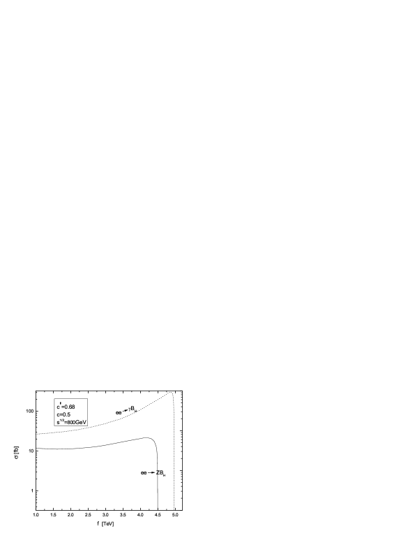
Figure 3: The cross sections of the processes $e^{+}e^{-}\rightarrow\gamma(Z)B_{H}$ as a function of the scale $f$, with $\sqrt{s}=800$ GeV, $c^{\prime}=0.68$, and $c$=0.5.

The mixing parameter $c$ only has a little effect on the masses of the final states $B_{H}$ and Z, so the cross sections are insensitive to the parameter $c$ and we fix c=0.5 as a example in our calculation.

In order to give more information about the $\gamma(Z)B_{H}$ productions, we also plot the angular distributions of these processes in Fig.4. Where $\theta$ is the angle between the incoming electron beams and the scattering $B_{H}$. The fig.4 shows that the angular distributions sharply increase when $cos\theta$ approaches 1 or -1 due to the t-channel resonance effect. This means that the $B_{H}$ signals are more concentrated near to the incoming $e^{+}e^{-}$ axis.

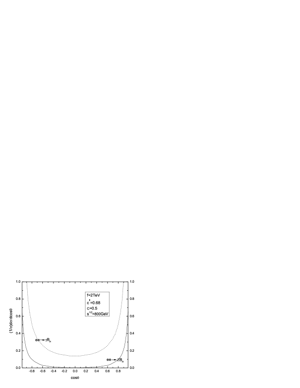
Figure 4: The angular distributions of the processes $e^{+}e^{-}\rightarrow\gamma(Z)B_{H}$, with $\sqrt{s}=800$ GeV, $c^{\prime}=0.68$, $c$=0.5, and $f=2$ GeV. Here $\theta$ is the angle between the outgoing gauge boson $B_{H}$ and the incoming electron.

As we have discussed above, with the integrated luminosity 500 $fb^{-1}$ at the ILC, a large number of $B_{H}$ can be produced via the processes $e^{+}e^{-}\rightarrow\gamma(Z)B_{H}$ in the wide range of parameter space of the LH model, specially for the process $e^{+}e^{-}\rightarrow\gamma B_{H}$. However, the event rate of $B_{H}$ identified not only depends on the cross section, but also depends on the reconstruction efficiencies of the decay channels of $B_{H}$. The final states of the $\gamma(Z)B_{H}$ productions should include two jets. One is photon jet or the jet decaying from Z(such jet should includes light quark pair or lepton pair). Another jet is just the final states decaying from $B_{H}$. Both $\gamma$ and $Z$ can be easily identified experimentally, and such identification is necessary which can depress the SM background efficiently. To identify $B_{H}$ from its final states, we also need to study the decay modes of $B_{H}$. The main decay modes of $B_{H}$ are $e^{+}e^{-}+\mu^{+}\mu^{-}+\tau^{+}\tau^{-},d\bar{d}+s\bar{s},u\bar{u}+c\bar{c},ZH,W^{+}W^{-}$. The decay branching ratios of these modes have been studied in referenceHan . Because the light lepton pairs $l^{+}l^{-}(l=e,\mu)$ are typically well isolated from all other particles with high efficiency and the number of $l^{+}l^{-}$ background events with such a high invariant mass is very small, the peak in the invariant mass distribution of $l^{+}l^{-}$ should be sensitive to the presence of $B_{H}$. So the decay modes $l^{+}l^{-}$ are the most ideal modes to detect $B_{H}$ in most case. For these leptonic decay modes, the final states of $\gamma B_{H}$ production should be $\gamma l^{+}l^{-}$. In this case, the main SM background arises from the process $e^{+}e^{-}\rightarrow\gamma Z$ with large production rate(at the level of a few pb for $\sqrt{s}=800$ GeVZr ), which can lead to similar multi-jet topologies. However, it should be very easy to distinguish $B_{H}$ from $Z$ by measuring the invariant mass distributions of the $l^{+}l^{-}$ because such invariant mass distributions between $B_{H}$ and $Z$ are significantly different. The measurement of this lepton pair invariant mass distributions can drastically reduce the background and the production mode $e^{+}e^{-}\rightarrow\gamma B_{H}\rightarrow\gamma l^{+}l^{-}$ can achieve a very clean SM background. For the production mode $e^{+}e^{-}\rightarrow ZB_{H}\rightarrow Zl^{+}l^{-}$, the main SM background arises from the processes $e^{+}e^{-}\rightarrow ZZ,ZH$. As we have mentioned above, $B_{H}$ can be easily distinguished from $Z$ via their decay modes $l^{+}l^{-}$, and the decay branching ratios of $H\rightarrow l^{+}l^{-}$ are very small. Therefore, a clean SM background can also be achieved if one detect $B_{H}$ via the production mode $e^{+}e^{-}\rightarrow ZB_{H}\rightarrow Zl^{+}l^{-}$. When the parameter $c^{\prime}$ is near $\sqrt{\frac{2}{5}}$, the couplings $B_{H}l^{+}l^{-}$ become decoupled and the decay modes $l^{+}l^{-}$ can not be used to detect $B_{H}$. In this case, the decay modes $W^{+}W^{-},ZH$ can provide a complementary method to probe $B_{H}$. The decay branching ratios of $W^{+}W^{-},ZH$ greatly increase when $c^{\prime}$ is near $\sqrt{\frac{2}{5}}$, and in this case we might assume enough $W^{+}W^{-}$ and $ZH$ signals to be produced with high luminosity. The decay mode $Z\rightarrow W^{+}W^{-}$ is of course kinematically forbidden in the SM but $H\rightarrow W^{+}W^{-}$ is the dominant decay mode with Higgs mass above 135 GeV(one or both of W is off-shell for Higgs mass below 2$M_{W}$). So the dominant background for the signal $ZW^{+}W^{-}$ arises from the Higgsstrahlung process $e^{+}e^{-}\rightarrow ZH\rightarrow ZW^{+}W^{-}$ which is at the order of tens fbZH-background . Such background would be serious if one can not distinguish the $W^{+}W^{-}$ invariant mass distribution between H and $B_{H}$. However, the signal $\gamma W^{+}W^{-}$ does not suffer from such large background problem which would be one advantage of the process $e^{+}e^{-}\rightarrow\gamma B_{H}$. For $B_{H}\rightarrow ZH$, the main final states of $B_{H}$ are $l^{+}l^{-}b\bar{b}$. Two b-jets reconstruct to the Higgs mass and a $l^{+}l^{-}$ pair reconstructs to the Z mass. On the other hand, the decay mode $ZH$ involves the off-diagonal coupling $HZB_{H}$ and the experimental precision measurement of such off-diagonal coupling is more easier than that of diagonal coupling. So, the decay mode $ZH$ would provide an ideal way to verify the crucial feature of quadratic divergence cancellation in Higgs mass, furthermore such signals would provide crucial evidence that an observed new gauge boson is of the type predicted in the little Higgs models. For the signal $\gamma ZH,~{}ZZH$, although the same final states can be produced via $e^{+}e^{-}$ collision in the SM, the cross sections of these processes in the SM are small and the feature that there exists a peak in the $ZH$ invariant mass distribution for the signal can further help one to depress such background.

In summary, with the mass in the range of hundreds GeV, the $U(1)$ gauge boson $B_{H}$ is the lightest one among the new gauge bosons in the LH model. Such particle would be accessible in the first running of the ILC and provide an earliest signal of the LH model. In this paper, we study the $B_{H}$ production processes associated with a SM gauge boson $Z$ or $\gamma$ via $e^{+}e^{-}$ collision, i.e., $e^{+}e^{-}\rightarrow\gamma(Z)B_{H}$. We find that the cross sections are very sensitive to the parameters $c^{\prime},f$ and the cross section of $\gamma B_{H}$ production is much larger than that of $ZB_{H}$ production. In a wide range of the parameter space, sufficient events can be produced to detect $B_{H}$ via these processes. The signals are more concentrated near to the incoming $e^{+}e^{-}$ axis. In most case, $B_{H}$ can be detected via its decay modes $e^{+}e^{-},\mu^{+}\mu^{-}$ which can provide the typical signal and clean background. Therefore, the processes $e^{+}e^{-}\rightarrow\gamma(Z)B_{H}$ would open an ideal window to probe $B_{H}$ with the high luminosity at the planned ILC. Furthermore, if such gauge boson is observed, the precision measurement is need which could offer the important insight for the gauge structure of the LH model and distinguish this model from alternative theories.

References

- (1) The LEP Collaborations and the LEP Electroweak Working Group, hep-ex/05011027.
- (2) For review, Dimopoulos and H. Georgi, Nucl. Phys. B193, 150(1981); H. P. Nilles, Phys. Rep. 110, 1(1984); H. E. Haber and G.L.Kane, ibid. 117, 75(1985).
- (3) I. Antoniadis, C. Munoz, and M. Quiros, Nucl. Phys. B397, 515(1999); N. Arkani-Hamed, S. Dimopoulos, and G. R. Dvali, Phys. Rev. D59, 086004(1999).
- (4) S. Weinberg, Phys. Rev. D13, 974(1976); ibid. D19, 1277(1979); L. Susskind, Phys. Rev. D20, 2619(1979).
- (5) N. Arkani-Hamed, A. G. Cohen, and H. Georgi, Phys. Lett. B513, 232(2001); N. Arkani-Hamed, A. G. Cohen, T. Gregoire, and J. G. Wacker, JHEP 0208, 020(2002); N. Arkani-Hamed, A. G. Cohen, E. Katz, A. E. Nelson, T. Gregoire, and J. G. Wacker, JHEP 0208, 021(2002); I. Low, W. Skiba, and D. Smith, Phys. Rev. D66, 072001(2002); M. Schmaltz, Nucl. Phys. Proc. Suppl. 117, 40(2003); W. Skiba and J. Terning, Phys. Rev. D68, 075001(2003).
- (6) N. Arkani-Hamed, A. G. Cohen, E. Katz, A. E. Nelson, JHEP 0207, 034(2002).
- (7) T. Han, H. E. Logan, B. McElrath, and L. T. Wang, Phys. Rev. D67, 095004(2003).
- (8) For examples, M. Perelstein, hep-ph/0512128; S. C. Park, J. Song, Phys. Rev. D69, 15010(2004); J. Hubisz and P. Meade, Phys.Rev. D71, 035016(2005); M. Schmaltz and D. Tucker-Smith, Ann.Rev.Nucl.Part.Sci. 55, 229(2005); T. Han, H. E. Logan, and L. T. Wang, JHEP 0601, 099(2006); W. Kilian and J. Reuter, Phys.Rev. D70, 015004 (2004); A. J. Buras, A. Poschenrieder, and S. Uhlig, hep-ph/0410309; M. Blanke, A. J. Buras, A.poschenrieder, S. Recksiegel, C. Tarantino, S. Uhlig, and A. Weiler, JHEP 0701, 066(2007).
- (9) V. I. Thlnov, Acta Phys. Polon. B37, 1049(2006); V. I. Telnov, Acta Phys. Polon. B37, 633(2006); M. Battaglia, T. Barklow, M. E. Peskin, Y. Okada, S. Yamashita, P. Zerwas, hep-ex/0603010.
- (10) J. A. Conley, J. Hewett, and M. P. Le, Phys. Rev. D72, 115014(2005).
- (11) C. X. Yue, L. Li, S. Yang, L. N. Wang, hep-ph/0610005; C. X. Yue, F. Zhang, L. N. Wang, L. Zhou, Phys.Rev. D72, 055008(2005).
- (12) X. L. Wang, J. H. Chen, Y. B. Liu, S. Z. Liu, H. Yang, Phys. Rev. D74, 015006(2006); X. L. Wang, Z. L. Jin, Q. G. Zeng, hep-ph/0701094.
- (13) A. J. Buras, A. Poschenrieder, S. Uhlig, and W. A. Bardeen, JHEP 0611, 062(2006).
- (14) C. Csaki, J. Hubisz, G.D. Kribs, P. Meade, J. Terning, Phys. Rev. D68, 035009(2003).
- (15) Mu-Chun Chen and S. Dawson, Phys. Rev. D70, 015003(2004); R. Casalbuoni, A. Deandrea, M. Oertel, JHEP 0402, 032(2004); J. L. Hewett, F. J. Petriello and T. G. Rizzo, JHEP 0310, 062(2003); C. Cs aki, J. Hubisz, G. D. Kribs, P. Meade, and J. Terning, Phys. Rev. D67 115002(2003).
- (16) T. Gregoire, D. R. Smith, and J. G. Wacker, Phys.Rev. D69, 115008(2004).
- (17) J. F. Donoghue, E. Golowich, and B. R. Holstein, Dynamics of the Standard Model, Cambridge Univiversity Press, 1992, P. 34.
- (18) S. Atag and I. Sahin, Phys.Rev. D70, 053014(2004).
- (19) E.Accomando et.al., Phys.Rep. 299, 1(1998).