Recent Developments in Neutrino Phenomenology

Abstract

The first phase of studies of the neutrino mass and mixing is essentially over. The outcome is the discovery of non-zero neutrino mass and determination of the dominant structure of the lepton mixing matrix. In some sense this phase was very simple, and nature was very collaborative with us: Two main effects - the vacuum oscillations and the adiabatic conversion in matter (the MSW-effect) - provide complete interpretation of the experimental results. Furthermore, with the present accuracy of measurements the $3\nu-$mixing analysis is essentially reduced to the $2\nu$ consideration. I will present a concise and comprehensive description of this first phase. The topics include: (i) the concept of neutrino mixing in vacuum and matter; (ii) physics of the oscillations and adiabatic conversion; (iii) the experimental evidences of the flavor transformations and determination of the oscillation parameters. Some implications of the obtained results are discussed. Comments are given on the next phase of the field that will be much more involved.

I Introduction

Recent major progress in neutrino phenomenology, and particle physics in general, was related to studies of the neutrino mass and mixing. The first phase of these studies is essentially over, with the main results being

• discovery of non-zero neutrino mass;

• determination of the dominant structure of the lepton mixing: discovery of two large mixing angles;

• establishing strong difference of the quark and lepton mass spectra and mixing patterns.

Physics of this first phase is rather simple. The two main effects - the vacuum oscillations pontosc ; mns ; pontprob and the adiabatic conversion in matter (the MSW-effect) w1 ; ms1 . are enough for complete interpretation of the experimental results. (Oscillations in matter appear as sub-leading statistically insignificant yet effect for the atmospheric and solar neutrino oscillations in the Earth.) Furthermore, at the present level of experimental accuracy the three neutrino analysis is essentially reduced to two neutrino analyzes, and degeneracy of parameters is practically absent. Nature was very “collaborative” with us, realizing the easiest possibilities and disentangling an interplay of various phenomena.

In a sense, we have now a “standard model of neutrinos” that can be formulated in the following way:

1). there are only three types of light neutrinos;

2). their interactions are described by the Standard electroweak theory;

3). masses and mixing are generated in vacuum; they originate from some high energy (short range) physics at the electroweak or/and higher scales.

Now the goal is to test these statements and to search for new physics beyond this “standard model”. Confirmation of the LSND result by MiniBooNE would be discovery of such a new physics.

The next phase of studies will be associated to new generation of neutrino experiments, which will start in 2008 - 2010. The main objectives of this new phase include determination the absolute scale of neutrino mass and sub-dominant structures of mixing: namely, 1-3 mixing, deviation of the 2-3 mixing from maximal value, the CP-violation phase(s). The objectives include also identification of neutrino mass hierarchy and precision measurements of already known parameters.

The next phase will be much more involved: New phenomena may show up at the sub-leading level. More complicated formalisms for their interpretation are required. Complete three-neutrino context of study will be the must. Severe problem of degeneracy of parameters appears.

In these lectures I will present a concise description of the first phase of studies of neutrino masses and mixing. I will start by a detailed discussion of the concept of neutrino mixing in vacuum and matter. In the second part, the the main effects involved: the vacuum oscillations, oscillations in matter and the adiabatic conversion, are described and physics derivation of all relevant formulas are given. In the third part I will present the experimental results and existing evidences of neutrino oscillations. For each experiment a simple analysis is described that allows one to evaluate the neutrino parameters without sophisticated global fit. This consideration is aimed at convincing that indeed, we see the oscillations and and our interpretation of results in terms of the vacuum masses and mixing is correct.

II Flavors, masses and mixing

II.1 Flavor mixing

The flavor neutrinos, $\nu_{f}\equiv(\nu_{e},\nu_{\mu},\nu_{\tau})$ are defined as the neutrinos that correspond to certain charge leptons: $e$, $\mu$ and $\tau$. The correspondence is established by the weak interactions: $\nu_{l}$ and $l$ ($l=e,\mu,\tau$) form the charged currents or doublets of the $SU_{2}$ symmetry group. Neutrinos, $\nu_{1}$, $\nu_{2}$, and $\nu_{3}$, with definite masses $m_{1}$, $m_{2}$, $m_{3}$ are the eigenstates of mass matrix as well as the eigenstates of the total Hamiltonian in vacuum.

The vacuum mixing means that the flavor states do not coincide with the mass eigenstates. The flavor states are combinations of the mass eigenstates:

$$\nu_{l}=U_{li}\nu_{i},~{}~{}~{}l=e,\mu,\tau,~{}~{}~{}i=1,2,3,$$ (1)

where the mixing parameters $U_{li}$ form the PMNS mixing matrix $U_{PMNS}$ pontosc ; mns . The mixing matrix can be conveniently parameterized as

$$U_{PMNS}=V_{23}(\theta_{23})I_{-\delta}V_{13}(\theta_{13})I_{\delta}V_{12}(\theta_{12}),$$ (2)

where $V_{ij}$ is the rotation matrix in the $ij$-plane, $\theta_{ij}$ is the corresponding angle and $I_{\delta}\equiv diag(1,1,e^{i\delta})$ is the matrix of CP violating phase.

II.2 Two aspects of mixing.

A number of conceptual points can be clarified using just $2\nu-$ mixing. Also, at the present level of accuracy of measurements the $2\nu-$ dynamics is enough to describe the data. For two neutrino mixing, e.g. $\nu_{e}-\nu_{a}$, we have

$$\nu_{e}=\cos\theta\nu_{1}+\sin\theta\nu_{2},~{}~{}\nu_{a}=\cos\theta\nu_{2}-\sin\theta\nu_{1},$$ (3)

where $\nu_{a}$ is the non-electron neutrino state, and $\theta$ is the vacuum mixing angle.

There are two important aspects of mixing. The first aspect: according to (3) the flavor neutrino states are combinations of the mass eigenstates. Propagation of $\nu_{e}$ ($\nu_{a}$) is described by a system of two wave packets which correspond to $\nu_{1}$ and $\nu_{2}$.

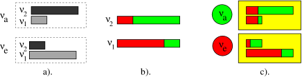
Figure 1: a). Representation of the flavor neutrino states as the combinations of the mass eigenstates. The length of the box gives the admixture of (or probability to find) corresponding mass state in a given flavor state. (The sum of the lengths of the boxes is normalized to 1. b). Flavor composition of the mass eigenstates. The electron flavor is shown by red (dark) and the non-electron flavor by green (grey). The sizes of the red and green parts give the probability to find the electron and non-electron neutrino in a given mass state. c). Portraits of the electron and non-electron neutrinos: shown are representations of the electron and non-electron neutrino states as combinations of the eigenstates for which, in turn, we show the flavor composition.

In fig. 1a). we show representation of $\nu_{e}$ and $\nu_{a}$ as the combination of mass states. The lengths of the boxes, $\cos^{2}\theta$ and $\sin^{2}\theta$, give the admixtures of $\nu_{1}$ and $\nu_{2}$ in $\nu_{e}$ and $\nu_{a}$. The key point is that the flavor states are coherent mixtures (combinations) of the mass eigenstates. The relative phase or phase difference of $\nu_{1}$ and $\nu_{2}$ in $\nu_{e}$ as well as $\nu_{a}$ is fixed: according to (3) it is zero in $\nu_{e}$ and $\pi$ in $\nu_{a}$. Consequently, there are certain interference effects between $\nu_{1}$ and $\nu_{2}$ which depend on the relative phase.

The second aspect: the relations (3) can be inverted:

$$\nu_{1}=\cos\theta~{}\nu_{e}-\sin\theta~{}\nu_{a},~{}~{}\nu_{2}=\cos\theta~{}\nu_{a}+\sin\theta~{}\nu_{e}.$$ (4)

In this form they determine the flavor composition of the mass states (eigenstates of the Hamiltonian), or shortly, the flavors of eigenstates. According to (4) the probability to find the electron flavor in $\nu_{1}$ is given by $\cos^{2}\theta$, whereas the probability that $\nu_{1}$ appears as $\nu_{a}$ equals $\sin^{2}\theta$. This flavor decomposition is shown in fig. 1b). by colors (different shadowing).

Inserting the flavor decomposition of mass states in the representation of the flavors states, we get the “portraits” of the electron and non-electron neutrinos fig. 1c). According to this figure, $\nu_{e}$ is a system of two mass eigenstates that, in turn, have a composite flavor. On the first sight the portrait has a paradoxical feature: there is the non-electron (muon and tau) flavor in the electron neutrino! The paradox has the following resolution: in the $\nu_{e}$- state the $\nu_{a}$-components of $\nu_{1}$ and $\nu_{2}$ are equal and have opposite phases. Therefore they cancel each other and the electron neutrino has pure electron flavor as it should be. The key point is interference: the interference of the non-electron parts is destructive in $\nu_{e}$. The electron neutrino has a “latent” non-electron component which can not be seen due to particular phase arrangement. However, during propagation the phase difference changes and the cancellation disappears. This leads to an appearance of the non-electron component in propagating neutrino state which was originally produced as the electron neutrino. This is the mechanism of neutrino oscillations. Similar consideration holds for the $\nu_{a}$ state.

II.3 Who mixes neutrinos?

How mixed neutrino states (that is, the coherent mixtures on the mass eigenstates) are created? Why neutrinos and not charged leptons? In fact, these are non-trivial questions. Creation (preparation - in quantum mechanics terms) of the mixed neutrino states is a result of interplay of the charged current weak interactions and kinematic features of specific reactions. Differences of masses of the charged leptons play crucial role.

Let us consider three neutrino species separately.

1). Electron neutrinos: The combination of mass eigenstates, which we call the electron neutrino, is produced, e.g., in the beta decay (together with electron). The reason is the energy conservation: no other combination can be produced because the energy release is about few MeV, so that neither muon nor tau lepton can appear.

2). Muon neutrino. Almost pure $\nu_{\mu}$ state is produced together with muons in the charged pion decay: $\pi^{+}\rightarrow\mu^{+}\nu_{\mu}$. Here the reason is “chirality suppression” - essentially the angular momentum conservation and V-A character of the charged current weak interactions. The amplitude is proportional to the mass of the charged lepton squared. Therefore the channel with the electron neutrino: $\pi^{+}\rightarrow e^{+}\nu_{e}$ is suppressed as $\propto m_{e}^{2}/m_{\mu}^{2}$. Also coherence between $\nu_{\mu}$ and small admixture of $\nu_{e}$ is lost almost immediately due to difference of kinematics.

3). Tau neutrino. Enriched $\nu_{\tau}$ - flux can be obtained in the beam-dump experiments at high energies: In the thick target all light mesons ($\pi$, $K$ which are sources of usual neutrinos) are absorbed before decay, and only heavy short living particles, like $D$ mesons, have enough time to decay. The $D$ mesons have also modes of decay with emission of $\nu_{e}$ and $\nu_{\mu}$ that are chirality-suppressed in comparison with $D\rightarrow\tau\nu_{\tau}$. Furthermore, coherence of $\nu_{e}$ and $\nu_{\mu}$ with $\nu_{\tau}$ is lost due to strongly different energies and momenta.

What about the neutral currents? Which neutrino state is produced in the $Z^{0}-$decay in the presence of mixing? $Z^{0}-$interactions are flavor blind and all the neutrino flavors are produced with the same amplitude (rate). The only characteristic that distinguishes neutrinos is the mass. So, the state produced in the $Z^{0}$-decay can be written as

$$|f\rangle=\frac{1}{\sqrt{3}}\left[|\bar{\nu}_{1}\nu_{1}\rangle+|\bar{\nu}_{2}\nu_{2}\rangle+|\bar{\nu}_{3}\nu_{3}\rangle\right]$$ (5)

(which is also equivalent to the sum of pairs of the flavor states) gt . It is straightforward to show that the decay rate $|Z^{0}\rangle\rightarrow|f\rangle$ is given by

$$|\langle f|H|Z^{0}\rangle|^{2}=3|\langle\bar{\nu}_{1}\nu_{1}|H|Z^{0}\rangle|^{2},$$ (6)

that coincides with what one obtains in the case of three independent decay channels.

Do neutrinos from $Z^{0}$-decay oscillate? One can show that oscillations can be observed in the two-detector experiments when both neutrinos from the decay are detected gt . If a flavor of neutrino (antineutrino) is fixed, then a flavor of the accompanying antineutrino (neutrino) will oscillate with distance and energy.

III Physics effects

III.1 To determination of oscillation parameters

In the Table 1 we show parameters to be determined, sources of information for their determination and the main physical effects involved. In the first approximation, when 1-3 mixing is neglected, the three neutrino problem splits into two neutrino problems and parameters of the 1-2 and 2-3 sectors can be determined independently.

Table 1: Parameters and effects.

Parameters	Source of information	Main physics effects
$\Delta m_{12}^{2}$, $\theta_{12}$	Solar neutrinos	Adiabatic conversion
		and averaged vacuum
		oscillations
	KamLAND	Non-averaged vacuum
		oscillations
$\Delta m_{23}^{2}$, $\theta_{23}$	Atmospheric neutrinos	Vacuum oscillations
	K2K	Vacuum oscillations
$\theta_{13}$	CHOOZ	Vacuum oscillations
	Atmospheric neutrinos	Oscillations in matter

Essentially two effects are relevant for interpretation of the present data in the lowest approximation:

• vacuum oscillations (both averaged and non-averaged)pontosc ; mns ; pontprob ;

• adiabatic conversion in medium w1 ; ms1 .

A priory another effect - oscillations in matter - should also be used in the analysis. It is relevant for the solar and atmospheric neutrinos propagating in the matter of the Earth. It happens however, that for various reasons the effect is small - at $(1-2)\sigma$ level and can be neglected in the first approximation.

In the case of solar neutrinos, for the preferable values of oscillation parameters of the LMA solution (see below) this effect is indeed small. Furthermore, due to the attenuation (see below) the Earth-core effect is small and one can consider oscillations as ones in constant density.

In the case of atmospheric neutrinos the $\nu_{e}-$ and $\nu_{\mu}-$ transition probabilities driven by 1-2 mixing and mass splitting are not small (of the order one in the sub-GeV range). However, due to an accidental coincidence (the fact that the ratio of the muon-to-electron neutrino fluxes equals 2) the effect cancels for maximal 2-3 mixing (see below).

Notice also that the $2\nu-$ mixing analyzes are enough. However, in the next order, when sub-leading effects are included, the problem becomes much more difficult and degeneracy of parameters appear. We will comment on this later.

III.2 Neutrino oscillation in vacuum

In vacuum, the neutrino mass states are the eigenstates of the Hamiltonian. Therefore dynamics of propagation has the following features:

• Admixtures of the eigenstates (mass states) in a given neutrino state do not change. In other words, there is no $\nu_{1}\leftrightarrow\nu_{2}$ transitions. $\nu_{1}$ and $\nu_{2}$ propagate independently. The admixtures are determined by mixing in a production point (by $\theta$, if pure flavor state is produced).

• Flavors of the eigenstates do not change. They are also determined by $\theta$. Therefore the picture of neutrino state (fig. 1 c) does not change during propagation.

• Relative phase (phase difference) of the eigenstates monotonously increases.

The phase is the only operating degree of freedom and we will consider it in details.

Phase difference. Due to difference of masses, the states $\nu_{1}$ and $\nu_{2}$ have different phase velocities $v_{phase}=E_{i}/p_{i}\approx 1+m_{i}^{2}/2E^{2}$ (for ultrarelativistic neutrinos), so that

$$\Delta v_{phase}\approx\frac{\Delta m^{2}}{2E^{2}},~{}~{}~{}\Delta m^{2}\equiv m_{2}^{2}-m_{1}^{2}.$$ (7)

The phase difference changes as

$$\phi=\Delta v_{phase}Et.$$ (8)

Explicitly, in the plane-wave approximation we have the phases of two mass states $\phi_{i}=E_{i}t-p_{i}x$. Apparently, the phase difference which determines the interference effect one should be taken in the same space-time point:

$$\phi\equiv\phi_{1}-\phi_{2}=\Delta Et-\Delta px.$$ (9)

Since $p=\sqrt{E^{2}-m^{2}}$, we have

$$\Delta p=\frac{dp}{dE}\Delta E+\frac{dp}{dm^{2}}\Delta m^{2}=\frac{1}{v_{g}}\Delta E-\frac{\Delta m^{2}}{2p},$$ (10)

where $v_{g}=dE/dp$ is the group velocity. Plugging (10) into (9) we obtain

$$\phi=\Delta E\left(t-\frac{x}{v_{g}}\right)+\frac{\Delta m^{2}}{2p}x.$$ (11)

Depending on physical conditions either $\Delta E\approx 0$ or/and $(t-x/v_{g})$ is small which imposes the bound on size of the wave packet. As a consequence, the first term is small and we reproduce the result (8). For stationary source one should take $\Delta E=0$.

In general, depending on conditions of production and detection both quantities $\Delta E$ and $\Delta p$ are non-zero. There is always certain time interval in the problem, $\Delta t$, that determines (according to the uncertainty principle) the energy interval $\Delta E$. E.g. in the case of solar neutrinos we know a time interval (determined by the time resolution of a detector) when a given neutrino is detected. Furthermore, neutrino production processes have certain life-times, or coherence times. There are arguments that one should take the center of the wave packet where $t=x/v_{g}$, or average over the wave packet length that leads to vanishing the first term in (11). In both cases one obtains standard expression for the phase. Apparently, the oscillation effect should disappear in the limit $\Delta m^{2}=0$.

Notice that oscillations are the effect in the configuration space. The process is described by interference of the wave functions that correspond to the mass eigenstates, $\psi_{1}(x,t)$ and $\psi_{2}(x,t)$. Formally, we can perform the Fourier expansion of these wave functions considering the interference in the momentum representation. So, formally we can always take the same momenta doing then appropriate integration.

Increase of the phase leads to the oscillations. Indeed, the change of phase modifies the interference: in particular, cancellation of the non-electron parts in the state produced as $\nu_{e}$ disappears and the non-electron component becomes observable. The process is periodic: when $\phi=\pi$, the interference of non-electron parts is constructive and at this point the probability to find $\nu_{a}$ is maximal. Later, when $\phi=2\pi$, the system returns to its original state: $\nu(t)=\nu_{e}$. The oscillation length is the distance at which this return occurs:

$$l_{\nu}=\frac{2\pi}{\Delta v_{phase}E}=\frac{4\pi E}{\Delta m^{2}}.$$ (12)

The depth of oscillations, $A_{P}$, is determined by the mixing angle. It is given by maximal probability to observe the “wrong” flavor $\nu_{a}$. From the fig. 1c. one finds immediately (summing up the parts with the non-electron flavor in the amplitude)

$$A_{P}=(2\sin\theta\cos\theta)^{2}=\sin^{2}2\theta.$$ (13)

Putting things together we obtain expression for the transition probability

$$P=A_{P}\left(1-\cos\frac{2\pi L}{l_{\nu}}\right)=\sin^{2}2\theta\sin^{2}\frac{\Delta m^{2}L}{4E}.$$ (14)

The oscillations are the effect of the phase increase which changes the interference pattern. The depth of oscillations is the measure of mixing.

III.3 Paradoxes of neutrino oscillations

A number of issues in theory of neutrino oscillations is still under discussion. Here I add several comments. Naive plane-wave description reproduces correct result since it catches the main feature of the effect: phase difference change. Clearly it can not explain whole the picture because the oscillations are a finite space-time effect.

Field theory approach provides with a consistent description. Oscillation experiment includes neutrino production in the source, propagation between the source and detector, detection. In this approach production, propagation and detection of neutrinos are considered as a unique process in which $\nu_{1}$ and $\nu_{2}$ are virtual particles propagating between the production, $x_{P}$, and detection, $x_{D}$, points. Propagation of $\nu_{i}$ ($i=1,2$) is described by propagators $S_{i}(x_{D}-x_{P})$. Notice that here there is a substantial difference from our standard calculations of the probabilities and cross-sections when we consider the asymptotic states and perform integration over the infinite space-time. The later leads to appearance of the delta-functions that express conservation of the energy and momentum. In the case of oscillations integration should be performed over finite production and detection regions (integration over $x_{P}$ and $x_{D}$). Also one should take into account finite accuracy of measurements of the energy and momenta of external particles.

From this point of view in usual consideration we perform truncation of whole process: For $|x_{P}-x_{D}|\gg 1/\Delta p$ neutrinos can be considered as real (on-shell) particles with negligible corrections due to virtuality. Whole the process can be truncated in three parts: 1). production; 2). propagation, as propagation of wave packets; 3). detection. Neutrino masses are neglected in the production and detection processes. In this picture, the oscillations are considered as the effect of propagation with certain initial and final conditions that reflect process of production and detection. (Their effects develop over much larger space-time intervals.) Correct boundary (initial and final) conditions should be imposed. Essentially these conditions determine the length and shape of the wave packets.

Let us stress again that oscillations are the finite space and finite time phenomenon: all the phases of the processes, production, propagation and detection occur (and should be considered) in the finite time intervals and finite regions of space.

III.4 Evolution equation

In vacuum the mass states are the eigenstates of Hamiltonian. So, their propagation is described by independent equations

$$i\frac{d\nu_{i}}{dt}=E_{i}\nu_{i}\approx\left(p_{i}+\frac{|m_{i}|^{2}}{2p_{i}}\right)\nu_{i},$$ (15)

where we have taken ultrarelativistic limit and omitted the spin variables that are irrelevant for the flavor oscillations. In the matrix form for three neutrinos $\nu\equiv(\nu_{1},\nu_{2},\nu_{3})^{T}$, we can write

$$i\frac{d\nu}{dt}\approx\left(pI+\frac{|M_{diag}|^{2}}{2E}\right)\nu,$$ (16)

where $M_{diag}^{2}=diag(m_{1}^{2},m_{2}^{2},m^{2}_{3})$. Using the relation $\nu=U_{PMNS}^{\dagger}\nu_{f}$ (1), we obtain the equation for the flavor states:

$$i\frac{d\nu_{f}}{dt}\approx\frac{M^{2}}{2E}\nu_{f},$$ (17)

where $M^{2}\equiv U_{PMNS}|M_{diag}|^{2}U_{PMNS}^{\dagger}$ is the mass matrix squared in the flavor basis. In (17) we have omitted the term proportional to the unit matrix which does not produce any phase difference and can be absorbed in the renormalization of the neutrino wave functions. So, the Hamiltonian of the neutrino system in vacuum is

$$H_{0}=\frac{|M|^{2}}{2E}.$$ (18)

In the $2\nu$ mixing case we have explicitly:

$$H_{0}=\frac{\Delta m^{2}}{4E}\left(\begin{array}[]{cc}-\cos 2\theta&\sin 2\theta\\ \sin 2\theta&\cos 2\theta\end{array}\right).$$ (19)

Solution of the equation (17) with this Hamiltonian leads to the standard oscillation formula (14).

III.5 Matter effect

Refraction. In matter, neutrino propagation is affected by interactions. At low energies the elastic forward scattering is relevant only (inelastic interactions can be neglected) w1 . It can be described by the potentials $V_{e}$, $V_{a}$. In usual medium difference of the potentials for $\nu_{e}$ and $\nu_{a}$ is due to the charged current scattering of $\nu_{e}$ on electrons ($\nu_{e}e\rightarrow\nu_{e}e$) w1 :

$$V=V_{e}-V_{a}=\sqrt{2}G_{F}n_{e}~{},$$ (20)

where $G_{F}$ is the Fermi coupling constant and $n_{e}$ is the number density of electrons. The result follows straightforwardly from calculation of the matrix element $V=\langle\Psi|H_{CC}|\Psi\rangle$, where $\Psi$ is the state of medium and neutrino. Equivalently, one can describe the effect of medium in terms of the refraction index: $n_{ref}-1={V}/{p}$.

The difference of the potentials leads to an appearance of additional phase difference in the neutrino system: $\phi_{matter}\equiv(V_{e}-V_{a})t$. The difference of potentials (or refraction indexes) determines the refraction length:

$$l_{0}\equiv\frac{2\pi}{V_{e}-V_{a}}=\frac{\sqrt{2}\pi}{G_{F}n_{e}}.$$ (21)

$l_{0}$ is the distance over which an additional “matter” phase equals $2\pi$.

In the presence of matter the Hamiltonian of system changes:

$$H_{0}\rightarrow H=H_{0}+V,$$ (22)

where $H_{0}$ is the Hamiltonian in vacuum. Using (18) we obtain (for $2\nu$ mixing)

$$H=\frac{|M|^{2}}{2E}+V,~{}~{}~{}~{}V=diag(V,0).$$ (23)

The evolution equation for the flavor states in matter then becomes

$$i\frac{d\nu_{f}}{dt}=\left[\frac{\Delta m^{2}}{4E}\left(\begin{array}[]{cc}-\cos 2\theta&\sin 2\theta\\ \sin 2\theta&\cos 2\theta\end{array}\right)+V\right]\nu_{f}.$$ (24)

The eigenstates and the eigenvalues change:

$$\nu_{1},~{}~{}\nu_{2}~{}~{}~{}\rightarrow~{}~{}~{}\nu_{1m},~{}~{}\nu_{2m},$$ (25)

$$\frac{m_{1}^{2}}{2E},~{}~{}\frac{m_{2}^{2}}{2E}~{}~{}\rightarrow~{}~{}H_{1m},~{}~{}H_{2m}.$$ (26)

The mixing in matter is determined with respect to the eigenstates of the Hamiltonian in matter, $\nu_{1m}$ and $\nu_{2m}$. Similarly to (3) the mixing angle in matter, $\theta_{m}$, gives the relation between the eigenstates in matter and the flavor states:

$$\nu_{e}=\cos\theta_{m}\nu_{1m}+\sin\theta_{m}\nu_{2m},$$

$$\nu_{a}=\cos\theta_{m}\nu_{2m}-\sin\theta_{m}\nu_{1m}.$$ (27)

The angle $\theta_{m}$ in matter is obtained by diagonalization of the Hamiltonian in matter (23):

$$\sin^{2}2\theta_{m}=\frac{\sin^{2}2\theta}{(\cos 2\theta-2VE/\Delta m^{2})^{2}+\sin^{2}2\theta}.$$ (28)

In matter both the eigenstates and the eigenvalues, and consequently, the mixing angle depend on matter density and neutrino energy. It is this dependence activates new degrees of freedom of the system and leads to qualitatively new effects.

Resonance. Level crossing. According to (28), the dependence of the effective mixing parameter in matter, $\sin^{2}2\theta_{m}$, on density, neutrino energy as well as the ratio of the oscillation and refraction lengths:

$$x\equiv\frac{l_{\nu}}{l_{0}}=\frac{2EV}{\Delta m^{2}}\propto En_{e}$$ (29)

has a resonance character. At

$$l_{\nu}=l_{0}\cos 2\theta~{}~{}~{}~{}~{}~{}~{}{\rm(resonance~{}~{}condition)}$$ (30)

the mixing becomes maximal: $\sin^{2}2\theta_{m}=1$. For small vacuum mixing the condition (30) reads:

$$Oscillation~{}~{}length\hskip 5.69046pt\approx\hskip 5.69046ptRefraction~{}~{}length.$$ (31)

That is, the eigen-frequency which characterizes a system of mixed neutrinos, $1/l_{\nu}$, coincides with the eigen-frequency of medium, $1/l_{0}$.

For large vacuum mixing ($\cos 2\theta_{12}=0.4-0.5$) there is a significant deviation from the equality (31). Large vacuum mixing corresponds to the case of strongly coupled system for which the shift of frequencies occurs.

The resonance condition (30) determines the resonance density:

$$n_{e}^{R}=\frac{\Delta m^{2}}{2E}\frac{\cos 2\theta}{\sqrt{2}G_{F}}~{}.$$ (32)

The width of resonance on the half of the height (in the density scale) is given by

$$2\Delta n_{e}^{R}=2n_{e}^{R}\tan 2\theta.$$ (33)

Similarly, one can introduce the resonance energy and the width of resonance in the energy scale.

In medium with varying density, the layer where the density changes in the interval

$$n_{e}^{R}\pm\Delta n_{e}^{R}$$ (34)

is called the resonance layer. In resonance, the level splitting (difference of the eigenstates $H_{2m}-H_{1m}$ ) is minimal cab ; bet and therefore the oscillation length being inversely proportional the level spitting, is maximal.

III.6 Soft neutrino masses

One possible deviation from the standard scenario can be related to existence of the “soft neutrino” masses or situation when a part of neutrino masses are soft. The neutrino masses can be generated by some low energy physics, so that the masses change with energy (distance) scale; also environment effect on the masses becomes substantial. Recently, such a possibility has been considered in the context of MaVaN scenario mavan . Neutrino mass is some function of a small VEV, $v$ of some new scalar field $m_{\nu}=m_{\nu}(v)$, and in turn, $v$ can depend on an environment, and in particular, on density of the background neutrinos (e.g. relic neutrinos). Another possibility is that the effective neutrino mass is generated by the exchange of light scalar boson that couples with usual matter (leptons and quarks). Scalar interactions lead to chirality-flip and therefore to generation ot true mass (and not just change of the dispersion relation as in the case of refraction.) Denoting the coupling constants of scalar boson with neutrinos and charged fermions by $\lambda_{\nu}$ and $\lambda_{f}$ correspondingly, we find the soft mass

$$m_{soft}=\frac{\lambda_{\nu}\lambda_{f}n_{f}}{m_{\phi}^{2}}.$$ (35)

So, in the evolution equation that describes oscillations one has

$$m_{\nu}=m_{vac}+m_{soft},$$ (36)

where $m_{vac}$ is a mass generated by some short range physics, e.g., the electroweak scale VEV.

III.7 Degrees of freedom

An arbitrary neutrino state can be expressed in terms of the instantaneous eigenstates of the Hamiltonian, $\nu_{1m}$ and $\nu_{2m}$, as

$$\nu(t)=\cos\theta_{a}\nu_{1m}+\sin\theta_{a}\nu_{2m}e^{i\phi}~{},$$ (37)

where

• $\theta_{a}=\theta_{a}(t)$ determines the admixtures of eigenstates in $\nu(t)$;
  

• $\phi(t)$ is the phase difference between the two eigenstates (phase of oscillations):

  $$\phi(t)=\int_{0}^{t}\Delta Hdt^{\prime}+\phi(t)_{T}~{},$$ (38)

  here $\Delta H\equiv H_{1m}-H_{2m}$. The integral gives the adiabatic phase and $\phi(t)_{T}$ can be related to violation of adiabaticity. It may also have a topological contribution (Berry phase) in more complicated systems;
  

• $\theta_{m}(n_{e}(t))$ determines the flavor content of the eigenstates: $\langle\nu_{e}|\nu_{1m}\rangle=\cos\theta_{m}$, etc..

Different processes are associated with these three different degrees of freedom.

III.8 Oscillations in matter. Resonance enhancement of oscillations

In medium with constant density the mixing is constant: $\theta_{m}(E,n)=const$. Therefore

• the flavors of the eigenstates do not change;

• the admixtures of the eigenstates do not change; there is no $\nu_{1m}\leftrightarrow\nu_{2m}$ transitions, $\nu_{1m}$ and $\nu_{2m}$ are the eigenstates of propagation;

• monotonous increase of the phase difference between the eigenstates occurs: $\Delta\phi_{m}=(H_{2m}-H_{1m})t$.

This is similar to what happens in vacuum. The only operative degree of freedom is the phase. Therefore, as in vacuum, the evolution of neutrino has a character of oscillations. However, values of the oscillation parameters (length, depth) differ from those in vacuum. They are determined by the mixing in matter and by the effective energy splitting in matter:

$$\sin^{2}2\theta\rightarrow\sin^{2}2\theta_{m},~{}~{}~{}~{}~{}~{}l_{\nu}\rightarrow l_{m}=\frac{2\pi}{H_{2m}-H_{1m}}.$$ (39)

For a given density of matter the parameters of oscillations depend on the neutrino energy which leads to characteristic modification of the energy spectra. Suppose a source produces the $\nu_{e}$- flux $F_{0}(E)$. The flux crosses a layer of length, $L$, with a constant density $n_{e}$ and then detector measures the electron component of the flux at the exit from the layer, $F(E)$.

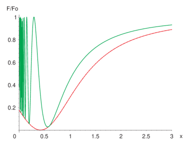
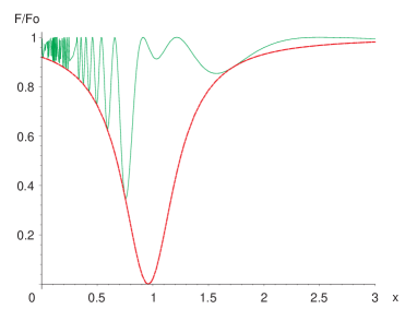
Figure 2:   Resonance enhancement of oscillations in matter with constant density. Shown is a dependence of the ratio of the final and original fluxes, $F/F_{0}$, on energy ($x\equiv l_{\nu}/l_{0}\propto E$) for a thin layer, $L=l_{0}/\pi$ (left panel) and thick layer $L=10l_{0}/\pi$ (right panel). $l_{0}$ is the refraction length. The vacuum mixing equals $\sin^{2}2\theta=0.824$.

In fig. 2 we show dependence of the ratio $F(E)/F_{0}(E)$ on energy for thick and thin layers. The oscillatory curve is inscribed in to the resonance curve $(1-\sin^{2}2\theta_{m})$. The frequency of the oscillations increases with the length $L$. At the resonance energy, the oscillations proceed with maximal depths. Oscillations are enhanced in the resonance range:

$$E=E_{R}\pm\Delta E_{R},~{}~{}~{}\Delta E_{R}=E_{R}\tan 2\theta=E_{R}^{0}\sin 2\theta,$$ (40)

where $E_{R}^{0}=\Delta m^{2}/2\sqrt{2}G_{F}n_{e}$. Notice that for $E\gg E_{R}$, matter suppresses the oscillation depth; for small mixing the resonance layer is narrow, and the oscillation length in the resonance is large. With increase of the vacuum mixing: $E_{R}\rightarrow 0$ and $\Delta E_{R}\rightarrow E_{R}^{0}$.

The oscillations in medium with nearly constant density are realized for neutrinos of different origins crossing the mantle of the Earth.

III.9 MSW: adiabatic conversion

In non-uniform medium, density changes on the way of neutrinos: $n_{e}=n_{e}(t)$. Correspondingly, the Hamiltonian of system depends on time, $H=H(t)$, and therefore,

(i) the mixing angle changes during propagation: $\theta_{m}=\theta_{m}(n_{e}(t))$;

(ii) the (instantaneous) eigenstates of the Hamiltonian, $\nu_{1m}$ and $\nu_{2m}$, are no more the “eigenstates” of propagation: the transitions $\nu_{1m}\leftrightarrow\nu_{2m}$ occur.

However, if the density changes slowly enough the transitions $\nu_{1m}\leftrightarrow\nu_{2m}$ can be neglected. This is the essence of the adiabatic condition: $\nu_{1m}$ and $\nu_{2m}$ propagate independently, as in vacuum or uniform medium.

Evolution equation for the eigenstates. Adiabaticity. Let us consider the adiabaticity condition. If external conditions (density) change slowly, the system (mixed neutrinos) has time to adjust this change.

To formulate this condition let us consider the evolution equation for the eigenstate of the Hamiltonian in matter. Inserting $\nu_{f}=U(\theta_{m})\nu_{m}$ in to equation for the flavor states (24) we obtain

$$i\frac{d\nu_{m}}{dt}=\left(\begin{array}[]{cc}H_{1m}&-i\dot{\theta}_{m}\\ i\dot{\theta}_{m}&H_{2m}\end{array}\right)\nu_{m}.$$ (41)

As follows from this equation for the neutrino eigenstates ms1 ; mess , $|\dot{\theta}_{m}|$ determines the energy of transition $\nu_{1m}\leftrightarrow\nu_{2m}$ and $|H_{2m}-H_{1m}|$ gives the energy gap between levels.

If mess

$$\gamma=\left|\frac{\dot{\theta}_{m}}{H_{2m}-H_{1m}}\right|\ll 1,$$ (42)

the off-diagonal terms can be neglected and system of equations for the eigenstates split. The condition (42) means that the transitions $\nu_{1m}\leftrightarrow\nu_{2m}$ can be neglected and the eigenstates propagate independently (the angle $\theta_{a}$ (37) is constant).

For small mixing angles the adiabaticity condition is crucial in the resonance layer where (i) the level splitting is small and (ii) the mixing angle changes rapidly. If the vacuum mixing is small, the adiabaticity is the most critical in the resonance point. It takes the form ms1

$$\Delta r_{R}>l_{R},$$ (43)

where $l_{R}=l_{\nu}/\sin 2\theta$ is the oscillation length in resonance, and $\Delta r_{R}=$ $n_{R}/(dn_{e}/dr)_{R}\tan 2\theta$ is the spatial width of resonance layer.

MSW- effect. Dynamical features of the adiabatic evolution can be summarized in the following way:

• The flavors of the eigenstates change according to density change. The flavor composition of the eigenstates is determined by $\theta_{m}(t)$.

• The admixtures of the eigenstates in a propagating neutrino state do not change (adiabaticity: no $\nu_{1m}\leftrightarrow\nu_{2m}$ transitions). The admixtures are given by the mixing in the production point, $\theta_{m}^{0}$.

• The phase difference increases; the phase velocity is determined by the level splitting (which in turn, changes with density (time)).

Now two degrees of freedom become operative: the relative phase and the flavors of neutrino eigenstates. The MSW effect is driven by the change of flavors of the neutrino eigenstates in matter with varying density. The change of phase produces the oscillation effect on the top of the adiabatic conversion.

Let us derive the adiabatic formula ms1 ; bet ; par ; hax . Suppose in the initial moment the state $\nu_{e}$ is produced in matter with density $n_{0}$. Then the neutrino state can be written in terms of the eigenstates in matter as

$$|\nu_{i}\rangle=|\nu_{e}\rangle=\cos\theta_{m}^{0}|\nu_{1m}\rangle+\sin\theta_{m}^{0}|\nu_{2m}\rangle,$$ (44)

where $\theta_{m}^{0}=\theta_{m}(n_{0})$ is the mixing angle in matter in the production point. Suppose this state propagates adiabatically to the region with zero density (as it happens in the case of the Sun). Then, the adiabatic evolution will consists of transitions $\nu_{1m}\rightarrow\nu_{1}$, $\nu_{2m}\rightarrow\nu_{2}$, and no transition between the eigenstates occurs, so the admixtures are conserved. As a result the final state is

$$|\nu(t)\rangle=\cos\theta_{m}^{0}|\nu_{1}\rangle+\sin\theta_{m}^{0}e^{i\phi(t)}|\nu_{2}\rangle,$$ (45)

where $\phi$ is the adiabatic phase. The survival probability is then given by

$$P=|\langle\nu_{e}|\nu(t)\rangle|^{2}.$$ (46)

Plugging $|\nu(t)\rangle$ (45) and $|\nu_{e}\rangle$ given by (3) into this expression and performing averaging over the phase which means that the contributions from $|\nu_{1}\rangle$ and $|\nu_{2}\rangle$ add incoherently, we obtain

$$P=(\cos\theta\cos\theta_{m}^{0})^{2}+(\sin\theta\sin\theta_{m}^{0})^{2}$$

$$=\sin^{2}\theta+\cos 2\theta\cos^{2}\theta_{m}^{0}.$$ (47)

This formula gives description of the solar neutrino conversion with accuracy $10^{-7}$, that is, corrections due to the adiabaticity violation are extremely small HLS .

Physical picture of the adiabatic conversion. According to the dynamical conditions, the admixtures of eigenstates are determined by the mixing in neutrino production point. This mixing in turn, depends on the density in the initial point, $n_{e}^{0}$, as compared to the resonance density. Consequently, a picture of the conversion depends on how far from the resonance layer (in the density scale) a neutrino is produced.

Figure 3:   Adiabatic evolution of neutrino state for three different initial condition ($n_{e}^{0}$). Shown are the neutrino states in different moments of propagation in medium with varying (decreasing) density. The yellow vertical line indicates position of resonance. The initial state is $\nu_{e}$ in all the cases. The sizes of the boxes do not change, whereas the flavors (colors) follow the density change.

Three possibilities relevant for solar neutrino conversion are shown in fig. 3. The state produced as $\nu_{e}$ propagates from large density region to zero density. Due to adiabaticity the sizes of boxes which correspond to the neutrino eigenstates do not change.

1). $n_{e}^{0}\gg n_{e}^{R}$: production far above the resonance (the upper panel). The initial mixing is strongly suppressed, and consequently, the neutrino state, $\nu_{e}$, consists mainly of one ($\nu_{2m}$) eigenstate, and furthermore, one flavor dominates in this eigenstate. In the resonance (its position is marked by the yellow line) the mixing is maximal: both flavors are present equally. Since the admixture of the second eigenstate is very small, oscillations (interference effects) are strongly suppressed. So, here we deal with the non-oscillatory flavor transition when the flavor of whole state (which nearly coincides with $\nu_{2m}$) follows the density change. At zero density we have $\nu_{2m}=\nu_{2}$, and therefore the probability to find the electron neutrino (survival probability) equals

$$P=|\langle\nu_{e}|\nu(t)\rangle|^{2}\approx|\langle\nu_{e}|\nu_{2m}(t)\rangle|^{2}=|\langle\nu_{e}|\nu_{2}\rangle|^{2}\approx\sin^{2}\theta.$$ (48)

This result corresponds to $\theta^{0}_{m}=\pi/2$ in formula (47).

The value of final probability, $\sin^{2}\theta$, is the feature of the non-oscillatory transition. Deviation from this value indicates a presence of oscillations.

2). $n_{e}^{0}>n_{e}^{R}$: production above the resonance (middle panel). The initial mixing is not suppressed. Although $\nu_{2m}$ is the main component, the second eigenstate, $\nu_{1m}$, has an appreciable admixture; also the flavor mixing in the neutrino eigenstates is significant. So, the interference effect is not suppressed. As a result, here an interplay of the adiabatic conversion and oscillations occurs.

3). $n_{e}^{0}<n_{e}^{R}$: production below the resonance (lower panel). There is no crossing of the resonance region. In this case the matter effect gives only corrections to the vacuum oscillation picture.

The resonance density is inversely proportional to the neutrino energy: $n_{e}^{R}\propto 1/E$. So, for the same density profile, the condition 1) is realized for high energies, the condition 2) is realized for intermediate energies and condition 3) – for low energies. As we will see all three case realize for solar neutrinos.

The adiabatic transformations show universality: The averaged probability and the depth of oscillations in a given moment of propagation are determined by the density in a given point and by initial condition (initial density and flavor). They do not depend on density distribution between the initial and final points. In contrast, the phase of oscillations is an integral effect of previous evolution and it depends on a density distribution.

The universal character of the adiabatic conversion can be further generalized in terms of variable ms1

$$y\equiv\frac{n_{e}^{R}-n_{e}}{\Delta n_{e}^{R}}$$ (49)

which is the distance (in the density scale) from the resonance density in the units of the width of resonance layer (33). In terms of $n$ the conversion pattern depends only on the initial value $y_{0}$.

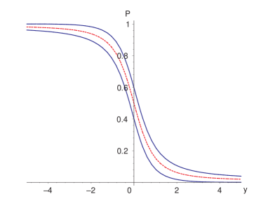
Figure 4: The dependence of the average probability (dashed line) and the depth of oscillations ($P^{max}$, $P^{min}$ solid lines) on $y$ for $y_{0}=-5$. The resonance layer corresponds to $y=0$. For $\tan^{2}\theta=0.4$ (large mixing MSW solution) the evolution stops at $y_{f}=0.47$.

In fig. 4 we show dependences of the average probability, $\bar{P}$, and depth of oscillations determined by $P^{max}$ and $P^{min}$, on $y$. The probability itself is the oscillatory function which is inscribed into the band shown by the solid lines. The average probability is shown by the dashed line. The curves are determined by the initial value $y_{0}$ only. In particular, there is no explicit dependence on the vacuum mixing angle. The resonance is at $y=0$ and the resonance layer is given by the interval $y=-1\div 1$. The figure corresponds to $y_{0}=-5$, i.e., to production above the resonance layer; the oscillation depth is relatively small. With further decrease of $y_{0}$, the oscillation band becomes narrower approaching the line of non-oscillatory conversion. For zero final density we have

$$y_{f}=\frac{1}{\tan 2\theta}.$$ (50)

So, the vacuum mixing enters the final condition. For the best fit LMA point, $y_{f}=0.45-0.50$, and the evolution should stop rather close top the resonance. The smaller mixing the larger final $y_{f}$ and the stronger transition.

III.10 Adiabaticity violation

In the adiabatic regime the probability of transition between the eigenstates is exponentially suppressed $P_{12}\sim exp{(-\pi/2\gamma)}$ and $\gamma$ is given in (42) hax ; par . One can consider such a transition as penetration through a barrier of the height $H_{2m}-H_{1m}$ by a system with the kinetic energy $d\theta_{m}/dt$.

If density changes rapidly, so that the condition (42) is not satisfied, the transitions $\nu_{1m}\leftrightarrow\nu_{2m}$ become efficient. Therefore the admixtures of the eigenstates in a given propagating state change. In our pictorial representation (fig. 3) the sizes of boxes change. Now all three degrees of freedom of the system become operative.

Typically, adiabaticity breaking leads to weakening of the flavor transition. The non-adiabatic transitions can be realized inside supernovas for the very small 1-3 mixing.

IV Determination of the oscillation parameters

IV.1 Solar neutrinos

Data. Data analysis is based on results from the Homestake experiment homestake , Kamiokande and SuperKamiokande sol05 , from radiochemical Gallium experiments SAGE sage , Gallex gallex and GNO gno and from SNO sno . The information we have collected can be described in three-dimensional space:

1. Type of events: $\nu e$ scattering (SK, SNO), CC-events (Cl, Ga, SNO) and NC events (SNO).

2. Energy of events: radiochemical experiments integrate effect over the energy from the threshold to the maximal energy in the spectrum. Also NC events are integrated over energies. The CC events in SNO and $\nu e$ events at SuperKamiokande give information about the energy spectrum of original neutrinos.

3. Time dependence of rates (searches for time variation of the flux).

Evidence of conversion. There are three types of observations which testify for the neutrino conversion:

1). Deficit of signal which implies the deficit of the electron neutrino flux. It can be described by the ratio $R\equiv N^{obs}/N^{SSM}$, where $N^{SSM}$ is the signal predicted according to the Standard solar model fluxes john . The deficit has been found in all (but SNO neutral current) experiments.

2). Energy spectrum distortion - dependence of the suppression factor on energy. Indirect evidence is provided by comparison of the deficits in experiments sensitive to different energy intervals:

$$Low~{}energies~{}(Ga):~{}~{}~{}R=0.5-0.6$$ (51)

$$High~{}energies~{}(Cl,~{}SK,~{}SNO):~{}~{}~{}R\approx 0.3.$$ (52)

So, the deficit increases with neutrino energy.

3). Smallness of ratio of signals due to charged currents and neutral currents sno :

$$\frac{CC}{NC}=0.340\pm 0.023~{}(stat.)~{}^{+0.029}_{-0.031}(syst.)~{}.$$ (53)

The latter is considered as the direct evidence of the flavor conversion since NC events are not affected by this conversion, whereas the number CC events is suppressed.

All this testifies for the LMA MSW solution.

Till now there is no statistically significant observations of other signatures of the conversion, namely,

- distortion of the boron neutrino spectrum: up turn at low energies in SK and SNO (significant effect should be seen below 5 - 7 MeV);

- day-night effect (recall that SK agrees with predictions however significance is about $1\sigma$);

- semiannual time variations on the top of annual variations (due to eccentricity of the Earth orbit).

Physics of conversion HSsol . Physics can be described in terms of three effects:

1). Adiabatic conversion (inside the Sun);

2). Loss of coherence of the neutrino state (on the way to the Earth);

3). Oscillations of the neutrino mass states in the matter of the Earth.

According to LMA, inside the Sun the initially produced electron neutrinos undergo the highly adiabatic conversion: $\nu_{e}\rightarrow\cos\theta_{m}^{0}\nu_{1}+\sin\theta_{m}^{0}\nu_{2}$, where $\theta_{m}^{0}$ is the mixing angle in the production point. On the way from the central parts of the Sun the coherence of neutrino state is lost after several hundreds oscillation lengths HSsol , and incoherent fluxes of the mass states $\nu_{1}$ and $\nu_{2}$ arrive at the surface of the Earth. In the matter of the Earth $\nu_{1}$ and $\nu_{2}$ oscillate partially regenerating the $\nu_{e}$-flux. With regeneration effects included the averaged survival probability can be written as

$$P=\sin^{2}\theta+\cos^{2}\theta_{12}^{m0}\cos 2\theta_{12}-\cos 2\theta_{12}^{m0}f_{reg}.$$ (54)

Here the first term corresponds to the non-oscillatory transition (dominates at the high energies), the second term is the contribution from the averaged oscillations which increases with decrease of energy, and the third term is the regeneration effect, with the regeneration factor, $f_{reg}$ defined as

$$f_{reg}\equiv P_{2e}-\sin^{2}\theta.$$ (55)

Here $P_{2e}$ is the probability of $\nu_{2}\rightarrow\nu_{e}$ transition in the matter of the Earth (without oscillations in matter: $P_{2e}=\sin^{2}\theta$). At low energies $P$ reduces to the vacuum oscillation probability with very small matter corrections.

There are three energy ranges with different features of transition:

1. In the high energy part of spectrum, $E>10$ MeV ($x\equiv l_{\nu}/l_{0}>2$), the adiabatic conversion with small oscillation effect occurs. At the exit, the resulting averaged probability is slightly larger than $\sin^{2}\theta$ expected from the non-oscillatory transition. With decrease of energy the initial density approaches the resonance density, and the depths of oscillations increases.

2. Intermediate energy range $E\sim(2-10)$ MeV ($x=0.3-2$ ) the oscillation effect is significant. The interplay of the oscillations and conversion takes place.

For $E\sim 2$ MeV neutrinos are produced in resonance.

3. At low energies: $E<2$ MeV ($x<0.3$), the vacuum oscillations with small matter corrections occur. The averaged survival probability $P\approx 0.5\sin^{2}2\theta$ is given by approximately the vacuum oscillation formula.

Inside the Earth. Entering the Earth the state $\nu_{2}$ (which dominates at high energies) splits in two matter eigenstates:

$$\nu_{2}\rightarrow\cos\theta_{m}^{\prime}\nu_{2m}+\sin\theta_{m}^{\prime}\nu_{1m}.$$ (56)

It oscillates regenerating partly the $\nu_{e}$-flux. In the approximation of constant density profile the regeneration factor equals

$$f_{reg}=0.5\frac{l_{\nu}}{l_{0}}~{}\sin^{2}2\theta=\frac{EV}{\Delta m^{2}}~{}\sin^{2}2\theta.$$ (57)

Notice that the oscillations of $\nu_{2}$ are pure matter effect and for the presently favored value of $\Delta m^{2}$ this effect is small. According to (57), $f_{reg}\propto 1/\Delta m^{2}$ and the expected day-night asymmetry of the charged current signal equals

$$A_{DN}=f_{reg}/P\sim(3-5)\%~{}.$$ (58)

Apparently the Earth density profile is not constant and it consists of several layers with slow density change and jumps of density on the borders between layers. It happens that for solar neutrinos one can get simple analytical result for oscillation probability for realistic density profile. Indeed, the solar neutrino oscillations occur in the so called low energy regime when

$$\epsilon\equiv\frac{2EV(x)}{\Delta m^{2}}\ll 1,$$ (59)

which means that the potential energy is much smaller than the kinetic energy. For the LMA oscillation parameters and the solar neutrinos: $\epsilon(x)=(1-3)\cdot 10^{-2}$. In this case one can use small parameter $\epsilon(x)$ (59) to develop the perturbation theory ara1 . The following expression for the regeneration factor, $f_{reg}$, has been obtained ara1 ; atv

$$f_{reg}=\frac{1}{2}\sin^{2}2\theta\int_{x_{0}}^{x_{f}}dxV(x)\sin\phi_{m}(x\rightarrow x_{f}).$$ (60)

Here $x_{0}$ and $x_{f}$ are the initial and final points of propagation correspondingly, and $\phi_{m}(x\rightarrow x_{f})$ is the adiabatic phase acquired between a given point of trajectory, $x$, and final point, $x_{f}$. The latter feature has important consequence leading to the attenuation effect - weak sensitivity to the remote structures of the density profile when non-zero energy resolution of detector is taken into account. On the other hand $f_{reg}$ can be strongly affected by some relatively small structures near the surface of the Earth.

Another insight into phenomena can be obtained using the adiabatic perturbation theory which leads to HLS

$$f_{reg}=\frac{2E\sin^{2}2\theta}{\Delta m^{2}}\sin\frac{\phi_{0}}{2}\sum_{j=0...n-1}\Delta V_{j}\sin\frac{\phi_{j}}{2}.$$ (61)

Here $\phi_{0}$ and $\phi_{j}$ are the phases acquired along whole trajectory and on the part of the trajectory inside the borders $j$. This formula corresponds to symmetric profile with respect to the center of trajectory. Using (61) one can easily infer the attenuation effect. The formula reproduces precisely the results of exact numerical calculations. Notice that the adiabatic perturbation theory is relevant here because the adiabaticity is fulfilled within the layers and maximally broken at the borders.

Determination of the solar oscillation parameters. Knowledge of the energy dependence of the adiabatic conversion allows one to connect the oscillation parameters with observables immediately.

1). Determination of the mixing angle. To explain stronger deficit at higher energies one needs to have $\theta<\pi/4$ or $\sin^{2}\theta<1/2$. Furthermore, using the fact that $P_{h}>\sin^{2}\theta$ and $P_{l}<0.5\sin^{2}2\theta$ we find

$$\frac{P_{h}}{P_{l}}\geq\frac{\sin^{2}\theta}{0.5\sin^{2}2\theta}=\frac{1}{2\cos^{2}\theta},$$ (62)

where on the RHS we have taken the asymptotic values of the survival probability. Consequently,

$$\sin^{2}\theta\leq 1-\frac{P_{l}}{2P_{h}}\sim 0.1\pm 0.2.$$ (63)

The ratio of CC to NC events determines the survival probability:

$$P=\sin^{2}\theta+\cos 2\theta\langle\cos^{2}\theta_{m}^{0}\rangle=\frac{CC}{NC}.$$ (64)

For high energies and without Earth matter regeneration effect $P=\sin^{2}\theta$. Since no significant distortion of the energy spectrum is seen at SK and SNO the Boron neutrino spectrum should be in the flat part (bottom of the “suppression pit”). In this region the deviation from asymptotic value is weak. For $\Delta m^{2}\sim 8\cdot 10^{-5}$ eV² the averaged oscillation effect is about $10\%$. Therefore

$$\sin^{2}\theta_{12}\approx 0.9\frac{CC}{NC}\approx 0.31.$$ (65)

2). Determination of $\Delta m^{2}$. Value of suppression in the Gallium experiments, $P_{l}$, implies that the $pp$- spectrum is in the vacuum dominated region, whereas stronger suppression of SK and SNO signals (together with an absence of distortion) means that the boron neutrino flux is in the matter dominated region. So, the transition region should be $E_{tr}\sim(1-4)$ MeV. On the other hand the expression for the middle energy of the transition region equals (it corresponds to neutrino production in resonance)

$$E_{tr}=\frac{\Delta m^{2}\cos 2\theta}{2V_{prod}},$$ (66)

where $V_{prod}$ is typical potential in the neutrino production region in the Sun. From (66) we obtain

$$\Delta m^{2}=\frac{2E_{tr}V_{prod}}{\cos 2\theta}$$ (67)

which gives $\Delta m^{2}=(3-15)\cdot 10^{-5}~{}~{}{\rm eV}^{2}$ in the correct range.

Another way to measure $\Delta m^{2}$ is to study the high energy effects: according to LMA the splitting $\Delta m^{2}$ is restricted from below by the increasing day-night asymmetry and from above by absence of the significant up turn of spectrum at low energies.

New SNO results are expected from the third (last) phase of the experiment that employs the ³He-counters for neutrons. The counters provide with a better identification of the NC-events and therefore preciser measurements of the CC/NC ratio, and the $\theta_{12}$ angle (combination of $\cos^{4}\theta_{13}\sin^{2}\theta_{12}$ in the three neutrino context). BOREXINO should start measurements soon borexino .

The SAGE calibration result is about $2\sigma$ below expectation calibr . That may testify for lower cross-section and therefore higher $pp-$flux at the earth due to larger survival probability. That produces some tension in the fit of the solar data fogli06 . Another possibility proposed recently is that the reduced calibration result is due to short range oscillations to sterile neutrinos giunti06 .

Searches for time variations and possible periodicity in the solar neutrino data are continued period .

IV.2 KamLAND

KamLAND (Kamioka Large Anti-neutrino detector) is the reactor long baseline experiment kamland . Few relevant details: 1kton liquid scintillator detector situated in the Kamioka laboratory detects the antineutrinos from surrounding atomic reactors (about 53) with the effective distance (150 - 210) km. The classical reaction of the inverse beta decay, $\bar{\nu}_{e}p\rightarrow e^{+}n$, is used. The data include

(i) the total rate of events;

(ii) the energy spectrum (fig. 5);

(iii) the time dependence of the signal which is due to variations of the reactors power. (Establishing the correlation between the neutrino signal and power of reactors is important check of the whole experiment). In fact, this change also influences the oscillation effect since the effective distance from the reactors changes (e.g., when power of the closest reactor decreases).

In the oscillation analysis the energy threshold $E>2.6$ MeV is established.

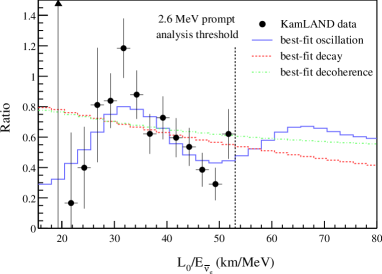
Figure 5: The $L/E$ distribution of events in the KamLAND experiment; from kamland .

The physics process is essentially the vacuum oscillations of $\bar{\nu}_{e}$. The matter effect, about $1\%$, is negligible at the present level of accuracy.

The evidences of the oscillations are

1). The deficit of the number of the $\bar{\nu}_{e}$ events

$$R_{\nu}=\frac{N_{obs}}{N_{expect}}=\frac{258}{365.2\pm 23.7}\sim 0.7$$ (68)

for $E>2.6$ MeV.

2). The distortion of the energy spectrum or $L/E$ dependence (when some reactors switch off the effective distance changes). Notice that an absence of strong spectrum distortion excludes large part of the oscillation parameter space.

Oscillation parameters are related to the observables in the following way. The main features of the $L/E$ dependence are maximum at $(L/E)_{max}=32$ km/MeV (phase $\phi=2\pi$) and minima at $L/E_{m}=16,~{}48$ km/MeV ($\phi=\pi,3\pi$). They fit well the expected oscillation pattern. Taking the first maximum we find

$$\Delta m^{2}=\frac{4\pi}{(L/E)_{max}}=8\cdot 10^{-5}~{}~{}{\rm eV}^{2}.$$

The deficit of the signal determines (for a given $\Delta m^{2}$) the value of mixing angle:

$$\sin^{2}2\theta_{12}=\frac{1-R_{\nu}}{\langle\sin^{2}\phi\rangle},$$ (69)

where the averaged over the energy interval oscillatory factor can be evaluated for the KamLAND detector as $\langle\sin^{2}\phi\rangle\sim 0.6$. Notice that sensitivity to mixing angle is not high at present.

Extracted values of the oscillation parameters are in a very good agreement with those obtained from the solar neutrino analysis. This comparison implies the CPT conservation.

Combined analysis of the solar neutrino data and the KamLAND can be performed in assumption of the CPT conservation. The mixing angle is mainly determined by the solar neutrino data, whereas $\Delta m^{2}$ is fixed by the KamLAND. New complete calibration of the detector will allow to improve sensitivity to 1-2 mixing KL-cal .

Comparison of results from the solar neutrinos and KamLAND open important possibility to check the theory of neutrino oscillation and conversion, test CPT, search for new neutrino interactions and new neutrino states.

IV.3 Atmospheric neutrinos

Experimental results. The atmospheric neutrino flux is produced in interactions of the high energy cosmic rays (protons, nuclei) with nuclei of atmosphere. The interactions occur at heights (10 - 20) km. At low energies the flux is formed in the chain of decays: $\pi\rightarrow\mu\nu_{\mu}$, $\mu\rightarrow e\nu_{e}\nu_{\mu}$. So, each chain produces $2\nu_{\mu}$ and $1\nu_{e}$, and correspondingly, the ratio of fluxes equals

$$r\equiv\frac{F_{\mu}}{F_{e}}\approx 2.$$ (70)

With increase of energy the ratio increases since the lifetime acquires the Lorentz boost and muons have no time to decay before collisions: they are absorbed or loose the energy. As a consequence, the flux of the electron neutrinos decreases.

In spite of the long term efforts, still the predicted atmospheric neutrino fluxes have large uncertainties (about 20% in overall normalization and about 5% in the so called “tilt” parameter which describes the uncertainty in the energy-dependence of the flux). The origin of uncertainties is twofold: original flux of the cosmic rays and cross sections of interactions.

The recent analyzes include the data from Baksan telescope, SuperKamiokande  atm ; tauapp , MACRO macro , SOUDAN soudan . The data can be presented in the three dimensional space which includes

- type of events detected: $e$-like events (showers), $\mu$-like events, multi-ring events, NC events (with detection of $\pi^{0}$), $\tau-$enriched sample of events.

- energy of events: widely spread classification includes the sub-GeV and multi-GeV events, stopping muons, through-going muons, etc..

- zenith angle (upward going, down going, etc).

Now MINOS experiment minos provides some early information on oscillation effects for the atmospheric neutrinos and antineutrinos separately.

The evidences of the atmospheric neutrino oscillations include:

1). Smallness of the double ratio of numbers of $\mu$-like to $e$-like events atm :

$$R_{\mu/e}\equiv\frac{N_{\mu}^{obs}/N_{\mu}^{th}}{N_{e}^{obs}/N_{e}^{th}}.$$ (71)

The ratio weakly depends on energy: it slightly increases from sub-GeV to multi-GeV range (as expected):

$$R_{\mu/e}=0.658\pm 0.016\pm 0.035~{}~{}{\rm(subGeV)}~{}~{}~{}~{}~{}~{}~{}~{}$$

$$R_{\mu/e}=0.702^{+0.032}_{-0.030}\pm 0.101~{}~{}{\rm(multiGeV+PC)}.$$ (72)

Apparently in the absence of oscillations (or other non-standard neutrino processes) the double ratio should be 1. The smallness of the ratio testifies for disappearance of the $\nu_{\mu}-$flux.

2). Distortion of the zenith angle dependence of the $\mu$ -like events (see fig. 6). Global characteristic of this distortion is the up-down asymmetry defined as

$$A_{up/down}\equiv\frac{N_{up}}{N_{down}}.$$ (73)

Due to complete up-down symmetric configuration for the production, in the absence of oscillations or other non-standard effects the asymmetry should be absent: $A_{up/down}=1$.

The zenith angle dependence for different types of events in different ranges of energies is shown in fig. 6 from atm . The zenith angle of the neutrino trajectory is related to the baseline $L$ as $L=D\cos\theta_{z}.$ So, studying the zenith angle distributions we study essentially the distance dependence of the oscillation probability.

Figure 6: The zenith angle distribution of the atmospheric $\mu$-like events in different energy ranges; from atm .

Substantial distortion of the zenith angle distribution is found. The deficit of numbers of events increases with decrease of $\cos\theta_{Z}$ and reaches about 1/2 in the upgoing vertical direction for multi-GeV events. The distortion increases with energy. Correspondingly, the up-down asymmetry increases with energy:

In contrast to the $\mu$-like, the $e$-like events distribution does not show any anomaly. Though one can mark some excess (about 15%) of the $e$-like events in the sub-GeV range (upper-left panel of fig. 6).

3). Appearance of the $\tau$-like events ($2.4\sigma$ effect) tauapp .

4). The $L/E-$dependence shows the first oscillation minimum (fig. 7).

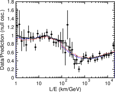
Figure 7: $L/E$ distribution of the atmospheric $\mu$ like events; from leatm . The solid line corresponds to the oscillation fit.

In the first approximation all these data can be consistently described in terms of the $\nu_{\mu}-\nu_{\tau}$ vacuum oscillations. Notice that for pure $2\nu$ oscillations of this type no matter effect is expected: the matter potentials of $\nu_{\mu}$ and $\nu_{\tau}$ are equal. In the context of three neutrino mixing, for non-zero values of $\sin\theta_{13}$ the matter effect should be taken into account for the $\nu_{\mu}-\nu_{\tau}$ channel.

As we marked above, the probabilities of $\nu_{e}$ and $\nu_{\mu}$ oscillations in matter of the Earth driven by the “solar” parameters $\Delta m^{2}_{21}$ and $\sin^{2}2\theta_{12}$ are large and even matter-enhanced in the sub-GeV range. However, observable effects of these oscillations are suppressed by factor

$$(r\cos^{2}\theta_{23}-1),$$ (74)

where the ratio $r$ is defined in eq. (70). In the sub-GeV range $r\approx 2$ and for maximal 2-3 mixing effects cancel. With increase of neutrino energy $r$ increases, however the probabilities are suppressed by matter effect.

So, in the first approximation a unique description in terms of $\nu_{\mu}-\nu_{\tau}$ oscillation is valid for different types of events and in a very wide range of energies: from 0.1 to more than 100 GeV.

Determination of the atmospheric neutrino oscillation parameters. Let us describe how the oscillation parameters can be immediately related to observables. We will use here the interpretation of the results in terms of $2\nu$-oscillations $\nu_{\mu}-\nu_{\tau}$.

The most clean way to determine parameters is to use the zenith angle distribution of the multi-GeV $\mu$-like events. As follows from fig. 6 for the down-going muons, $\cos\theta_{Z}\sim 0.5\div 1$, the oscillation effects are negligible (good agreement with the no-oscillation predictions). For the up-going muons, $\cos\theta_{Z}\sim-0.5\div-1$, there is already the averaging oscillation effect. Transition region corresponds to the horizontal events with $\cos\theta_{Z}\sim 0.0\div 0.2$. For these events the baseline $L=500$ km should be comparable with the oscillation length $L\approx l_{\nu}$, so that

$$\Delta m^{2}=\frac{4\pi E_{multi-GeV}}{L_{horizon}}.$$ (75)

Taking $E=(1-2)$ GeV we find $\Delta m^{2}=(1-4)\cdot 10^{-3}$ eV². An uncertainty in the neutrino direction and the fact that distance strongly depends on $\cos\theta_{Z}$ in the horizontal direction lead to the uncertainty in the determination of the atmospheric $\Delta m^{2}$.

For the upward-going $\mu$-like events the oscillations are averaged (no dependence of the suppression factor on $\cos\theta_{Z}$), so that $N^{obs}(up)/N^{th}(up)=1-\sin^{2}2\theta$. This allows us to determine the mixing angle:

$$\sin^{2}2\theta=2[1-N^{obs}(up)/N^{th}(up)].$$ (76)

  From the fig. 6 $N^{obs}(up)/N^{th}(up)\approx 0.5$, and consequently, $\sin^{2}2\theta=1$ ($N^{th}(up)\approx N^{obs}(up)$).

Other independent determinations are possible: in the sub-GeV range the zenith angle dependence is weak because of strong averaging effect: (i) the oscillation length is shorter and therefore the oscillations develop already for large part of the downgoing events; (ii) the angle between neutrino and detected muon is very large and directionality is essentially lost. So, taking the deficit of the total number of events we obtain

$$\sin^{2}2\theta\geq 2[1-R],$$ (77)

where equality corresponds to the developed oscillations for all directions. From fig. 6 we find $R=0.67$, and therefore $\sin^{2}2\theta\geq 0.7$.

To determine mixing angle one can use also the double ratio. As follows from (71)

$$\sin^{2}2\theta=\frac{1-R_{\mu/e}}{\langle\sin^{2}\phi/2\rangle_{z}},$$ (78)

where $\langle\sin^{2}\phi/2\rangle_{z}$ is the averaged over the energy and zenith angle oscillatory factor. For multi-GeV events $\langle\sin^{2}\phi/2\rangle_{z}=0.20-0.25$ and therefore from (78) we obtain $\sin^{2}2\theta\sim 1$.

The most precise determination of $\Delta m^{2}$ follows from the $L/E$ - dependence of the events (fig. 7) which is considered as the direct observation of the neutrino oscillations - oscillatory effect leatm . In the first oscillation minimum - dip in the survival probability the phase of oscillations equals $\phi=\pi$. Therefore

$$\Delta m^{2}=\frac{2\pi}{(L/E)_{dip}}.$$ (79)

From fig. 7: $(L/E)_{dip}=500$ km/GeV. This gives immediately $\Delta m^{2}=2.5\cdot 10^{-3}$ eV².

Results of the $3\nu-$analysis from concha and bari show one important systematic effect: the shift of 2-3 mixing from maximal one when the effect of the 1-2 sector is included. Also whole allowed region is shifted. Even larger deviation of $\sin^{2}\theta_{23}$ from 0.5 has been found in bari . Essentially this result is related to the excess of the $e$-like events in the sub-GeV range.

IV.4 K2K

The $\nu_{\mu}-$ beam with typical energies $E=(0.5-3)$ GeV was created at KEK and directed to Kamioka. Its interations were detected by SuperKamiokande k2k . The baseline is about 250 km. The oscillations of muon neutrinos, $\nu_{\mu}\rightarrow\nu_{\mu}$, have been studied by comparison of the detected number and the energy spectrum of the $\mu$-like events with the predicted ones. The predictions have been made by extrapolating the results from the “front” detector to the Kamioka place. The front detector similar to SK (but of smaller scale) was at about 1 km distance from the source.

The evidences of oscillations were (i) the deficit of the total number of events: 107 events have been observed whereas $151^{+12}_{-10}$ have been expected; (ii) the spectrum distortion (fig. 8). Searches for the $\nu_{\mu}\rightarrow\nu_{e}$ oscillations gave negative result.

The data are interpreted as the non-averaged vacuum oscillations $\nu_{\mu}-\nu_{\tau}$.

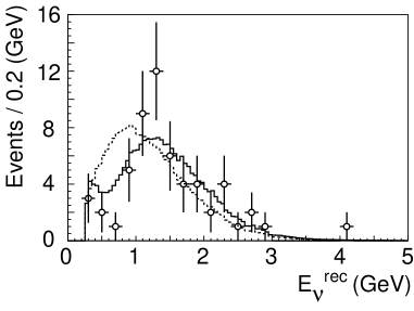
Figure 8: The energy spectrum of events in the K2K experiment, from k2k . Also shown are equally normalized fit curves with oscillations (solid) and without oscillations (dotted)

The energy distribution of the detected $\mu-$like events show an evidence of the first oscillation dip at $E\sim 0.5$ GeV (see fig. 8). This allows one to evaluate $\Delta m^{2}$. Using the relation (79) with $L/E=250{\rm km}/0.5{\rm GeV}=500$ km/GeV (apparently the same as in the atmospheric neutrino case), we obtain $\Delta m^{2}=2.5\cdot 10^{-3}$ eV² in perfect agreement with the atmospheric neutrino result. (In fact the data stronger exclude other values of $\Delta m^{2}$ than favor the best one.)

The substantial oscillation suppression is present in the low energy part of the spectrum ($E<1$ GeV) only. Therefore the deficit of events $\sim 0.67$ corresponds to large or nearly maximal mixing.

IV.5 MINOS

MINOS (Main Injector Neutrino Oscillation Search) is the long baseline experiment “from Fermilab to SOUDAN”. NuMI (Main Injector) beam consists, mainly, of $\nu_{\mu}$’s with energies (1 - 30) GeV and the flux-maximum at $\sim 3$ GeV. There are two detectors - steel-scintillator tracking calorimeters. The near detector is at the distance 1 km from the injector with mass 1 kton and the far detector (SOUDAN mine) has the baseline 735 km and mass 5.4 kt. The first result corresponds to exposure $1.27\cdot 10^{20}$ protons on target. 215 neutrino events have been observed below 30 GeV, whereas $336.0\pm 14.4$ events were predicted on the basis of measurements in the near detector minos-osc .

Evidence of oscillations consists of (i) deficit of the detected number of events - disappearance of the $\nu_{\mu}$-flux, and (ii) distortion of energy spectrum fig. 9. The relative suppression increases with decrease of energy (although there is large spread of points), and the strongest suppression is in the bins (1 - 2) GeV.

The dominant effect is the non-averaged vacuum $\nu_{\mu}-\nu_{\tau}$ oscillations. The m atter effect is negligible. Taking $E\sim 1.5$ GeV as the energy of the first oscillation dip (minimum) we find $\Delta m^{2}\sim(2.5-3.0)\cdot 10^{-3}$ eV². Suppression in this bin is consistent with maximal mixing. Using the total deficit of events one can evaluate the mixing angle more precisely.

Essentially we observe the high energy part of the first oscillation deep starting from minimum which is consistent with maximal suppression. This is enough to make rather precise determination of $\Delta m^{2}$. Detailed statistical fit gives $\Delta m^{2}_{23}=2.74^{+0.44}_{-0.26}\times 10^{-3}$ eV² (68 % C.L.) and $\sin^{2}2\theta_{23}>0.87$ (68 % C.L.) with the best fit value $\sin^{2}2\theta_{23}=1$. This is in a very good agreement with the atmospheric neutrino and K2K results.

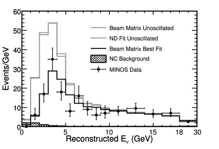
Figure 9: The energy spectrum of events in the MINOS experiment, from minos-osc . Shown also are the expected spectrum without oscillations and the best fit to experimental result.

Comment. Simple relations we have presented in sect. 4.1 - 4.5 allow us to understand where sensitivity to different parameters comes from. These relations are embedded in precise statistical analysis. They allow us to control the outcome of this analysis, understand uncertainties and give confidence in the results of more sophisticated analysis.

They show robustness of the results and their interpretation.

IV.6 1-3 mixing: effects and bounds

The direct bounds on 1-3 mixing are obtained in the CHOOZ experiment CHOOZ . This is the experiment with a single reactor, single detector and the baseline about 1 km. The expected effect is the vacuum non-average oscillations with survival probability given by the standard oscillation formula:

$$P=1-\sin^{2}2\theta_{13}\sin^{2}\frac{\phi}{2}.$$ (80)

The baseline is comparable with the half-oscillation length: For the best fit value of $\Delta m^{2}$ from the atmospheric neutrino studies and $E\sim 2$ MeV the oscillation length equals $\sim 2$ km.

The signature of the oscillations consists of distortion of the energy spectrum described by (80). No distortion has been found within the error bars which put the limit

$$\sin^{2}\theta_{13}\leq 0.04,~{}~{}(90\%~{}{\rm C.L.})$$ (81)

for $\Delta m^{2}_{31}=2.6\cdot 10^{-3}~{}{\rm eV}^{2}$. In the atmospheric neutrinos the non-zero 1-3 mixing will lead to oscillations of the electron neutrinos. One of the effects would be $\nu_{\mu}\leftrightarrow\nu_{e}$ oscillations in the matter of the Earth. The resonance enhancement of oscillations in neutrino or antineutrino channels should be observable depending on the type of mass hierarchy. That can produce an excess of the $e$-like events mostly in multi-GeV range where the mixing can be matter enhanced. No substantial effect is found. Notice that in the analysis bari - the best fit value $\sin\theta_{13}$ is non-zero due to some distortion of the zenith angle dependence. in the multi-GeV range.

In solar neutrinos, the non-zero 1-3 mixing leads to the averaged vacuum oscillations with small oscillation depth. The effect is reduced to change of the overall normalization of the flux. The combined analysis of all solar neutrino data leads to zero best-fit value of 1-3 mixing. The CC/NC ratio at SNO and Gallium results (which depend on the astrophysical uncertainties less) give $\sin^{2}\theta_{13}=0.017\pm 0.026$ (that indicates a level of sensitivity of existing observations).

In contrast, $\theta_{13}$ can produce leading effects for supernova electron (anti) neutrinos.

IV.7 Degeneracy of oscillation parameters and global fits

In the previous sections we have analyzed various data in the $2\nu$ context. Essentially the $3\nu$ system splits in to two sectors: “solar” sector probed by the solar neutrino experiments and KamLAND, and the “atmospheric” sector probed by the atmospheric neutrino experiments K2K and MINOS. This is justified if the 1-3 mixing is zero or small and if in the atmospheric sector studies the effect of 1-2 sector can be neglected. That could happen, e.g., because in the specific experiments the baselines are small or the energies are large, so that oscillation effects due to 1-2 mixing and 1-2 split have no time (space) to develop.

In the next phase of studies when sub-leading effects, e.g., induced by $\sin\theta_{13}$, become important the splitting of $3\nu$ problem into two sectors is not possible. At this sub-leading level the problem of determination of the neutrino parameters becomes much more complicated.

Table 2: Experiments and relevant oscillation parameters.

Experiments	Parameters of	Parameters of
	leading effects	sub-leading effects
Solar neutrinos,	$\Delta m^{2}_{12}$, $\theta_{12}$	$\theta_{13}$
KamLAND
Atmospheric neutrinos	$\Delta m^{2}_{23}$, $\theta_{23}$	$\Delta m^{2}_{12}$, $\theta_{12}$, $\theta_{13}$, $\delta$
K2K	$\Delta m^{2}_{23}$, $\theta_{23}$	$\theta_{13}$
CHOOZ	$\Delta m^{2}_{23}$, $\theta_{13}$	strongly suppressed
MINOS	$\Delta m^{2}_{23}$, $\theta_{23}$	$\theta_{13}$

In the table 2 we indicate relevant parameters for different studies. The same observables depend on several parameters, so that the problem of degeneracy of the parameters appears. In such a situation one needs to perform the global fit of all available data. The advantages are (1) no information is lost; (2) dependence of different observables on the same parameters is taken into account; (3) correlation of parameters and their degeneracy is adequately treated.

There are however some disadvantages. In particular, for some parameters the global fit may not be the most sensitive method, and certain subset of the data can restrict a given parameter much better (e.g., $\Delta m^{2}_{23}$ in atmospheric neutrinos).

In fig. 10 we show the results of the global fit of oscillation data performed in bari before MINOS results. MINOS shifts the allowed region and the best fit point of $\Delta m^{2}_{23}$ to larger values. With earlier MINOS result $\Delta m^{2}_{23}=2.6\cdot 10^{-3}~{}~{}{\rm eV}^{2}$ is found in  valencia as the best fit value.

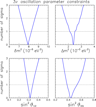
Figure 10: The results of global $3\nu$ analysis for 1-2 and 2-3 mass splits and mixings; from bari .

Results of global fits of the other groups (see sv ; valencia ) agree very well. Different types of experiments confirm each other: KamLAND confirms solar neutrino results, K2K - the atmospheric neutrino results etc.. Furthermore, unique interpretation of whole bulk of the data in terms of vacuum masses and mixings provides with the overall confirmation of the picture So, the determination of the parameters is rather robust, and it is rather non-plausible that future measurements will lead to significant change.

The most probable values of parameters equal

$$\Delta m^{2}_{12}=(7.9-8.0)\cdot 10^{-5}~{}~{}{\rm eV}^{2},$$ (82)

$$\sin^{2}\theta_{12}=0.310-0.315,~{}~{}~{}~{}~{}~{}~{}~{}~{}~{}~{}~{}~{}$$ (83)

$$\Delta m^{2}_{23}=(2.5-2.6)\cdot 10^{-3}~{}~{}{\rm eV}^{2}$$ (84)

$$\sin^{2}\theta_{23}=0.44-0.50.~{}~{}~{}~{}~{}~{}~{}~{}~{}~{}~{}~{}~{}~{}~{}$$ (85)

Slightly smaller value of 1-2 mixing, $\sin^{2}\theta_{12}=0.30$, has been found invalencia .

The parameter which describes the deviation of the 23 mixing from maximal equals

$$D_{23}\equiv 0.5-\sin^{2}\theta_{23}=0.03-0.06.$$ (86)

For 1-3 mixing we have

$$\sin^{2}\theta_{23}=0.00-0.01,~{}~{}~{}(1\sigma=0.011-0.013).$$ (87)

The ratio of mass squared differences important for theoretical implications equals

$$r_{\Delta}\equiv\frac{\Delta m^{2}_{12}}{\Delta m^{2}_{23}}=0.031-0.033.$$ (88)

V Neutrino mass and flavor spectrum

V.1 Spectrum

Information obtained from the oscillation experiments allows us to make significant progress in reconstruction of the neutrino mass and flavor spectrum (Fig. 11).

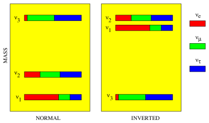
Figure 11: Neutrino mass and flavor spectra for the normal (left) and inverted (right) mass hierarchies. The distribution of flavors (colored parts of boxes) in the mass eigenstates corresponds to the best-fit values of mixing parameters and $\sin^{2}\theta_{13}=0.05$.

The unknowns are:

(i) admixture of $\nu_{e}$ in $\nu_{3}$, $U_{e3}$;

(ii) type of mass spectrum: hierarchical, non-hierarchical with certain ordering, degenerate, which is related to the value of the absolute mass scale, $m_{1}$;

(iii) type of mass hierarchy (ordering): normal, inverted (partially degenerate);

(iv) CP-violation phase $\delta$.

Information described in the previous sections can be summarized in the following way.

1. The observed ratio of the mass squared differences (88) implies that there is no strong hierarchy of neutrino masses:

$$\frac{m_{2}}{m_{3}}>\sqrt{\frac{\Delta m^{2}_{12}}{\Delta m^{2}_{23}}}=0.18\pm 0.02.$$ (89)

For charge leptons the corresponding ratio is 0.06, and even stronger hierarchies are observed in the quark sector.

2. There is the bi-large or large-maximal mixing between the neighboring families (1 - 2) and (2 - 3). Still rather significant deviation of the 2-3 mixing from the maximal one is possible.

3. Mixing between remote (1-3) families is weak.

To a good approximation the mixing matrix has the so-called tri-bimaximal form tbm :

$$U_{tbm}\equiv U_{23}^{m}U_{12}(\theta_{12})=\frac{1}{\sqrt{6}}\left(\begin{array}[]{ccc}2&\sqrt{2}&0\\ -1&\sqrt{2}&\sqrt{3}\\ 1&-\sqrt{2}&\sqrt{3}\end{array}\right),$$ (90)

where $U_{23}^{m}$ is the maximal ($\pi/4$) rotation in the 2-3 plane and $\sin^{2}\theta_{12}=1/3$. Alternatively, the mixing can be expressed in terms of the quark-lepton complementarity (QLC) relations qlc :

$$``{\rm lepton~{}mixing}={\rm bi-maximal~{}mixing}-{\rm CKM}^{\prime\prime}.$$ (91)

Possible realizations are

$$U_{PMNS}=U_{bm}U_{CKM}^{\dagger},{\rm or}$$

$$U_{PMNS}=U_{CKM}U_{bm}~{}~{}~{}$$ (92)

where $U_{CKM}$ is the quark mixing matrix and $U_{bm}$ is the bi-maximal mixing matrix:

$$U_{bm}\equiv U_{23}^{m}U_{12}^{m}=\frac{1}{2}\left(\begin{array}[]{ccc}\sqrt{2}&\sqrt{2}&0\\ -1&1&\sqrt{2}\\ 1&-1&\sqrt{2}\end{array}\right).$$ (93)

Both the tri-bimaximal mixing and the QLC-mixing agree with the experimental data within $1\sigma$ smsm .

V.2 Absolute scale of neutrino mass

Direct kinematic methods. Measurements of the Curie plot of the ${}^{3}H$ decay at the end point - give $m_{e}<2.05~{}{\rm eV}~{}~{}(95\%)$ (Troitsk) after “anomaly” subtraction troitsk , and $m_{e}<2.3~{}{\rm eV}~{}~{}(95\%)$, (Mainz) mainz . Future KATRIN experiment katrin aims at one order of magnitude better upper bound: $m_{e}<0.2~{}{\rm eV}~{}~{}(90\%)$. The discovery potential is estimated so that the positive result $m_{e}=0.35$ eV can be established at $5\sigma$ (statistical) level.

From oscillation experiments we get the lower bound on mass of the heaviest neutrino:

$$m_{h}>\sqrt{\Delta m^{2}_{atm}}=0.04~{}{\rm eV}~{}~{}~{}(95\%).$$ (94)

In the case of normal mass hierarchy $m_{h}=m_{3}$ and in the inverted hierarchy case $m_{h}=m_{1}\approx m_{2}$.

Neutrinoless double beta decay. The rate neutrinoless double beta decay is determined by the effective Majorana mass of electron neutrino

$$m_{ee}=\left|\sum_{k}U_{ek}^{2}m_{k}e^{i\phi(k)}\right|,$$ (95)

$\Gamma\propto m_{ee}^{2}$. Here $\phi(k)$ is the phase of the $k$ eigenvalue.

The best present bound on $m_{ee}$ is given by the Heidelberg-Moscow experiment: $m_{ee}<0.35-0.50$ eV HM-neg . Part of collaboration claims an evidence of a positive signal HM-pos ; hm . The Heidelberg-Moscow collaboration searched for the mode of the decay

$${}^{76}Ge\rightarrow^{76}Se+e^{-}+e^{-}$$ (96)

with the end point $Q_{ee}=2039$ keV. The total statistics collected from 5 enriched $Ge-$detectors is 71.7 kg yr. The peak at the end point of the total energy-spectrum of two electrons has been found and interpreted in hm as due to the neutrinoless double beta decay. Number of events in the peak gives the half-lifetime

$$T_{1/2}=1.19\cdot 10^{25}~{}{\rm y},~{}~{}~{}~{}~{}3\sigma~{}{\rm range}:(0.69-4.18)\cdot 10^{25}~{}~{}{\rm y}.$$ (97)

The significance of the peak depends on model of background and quoted by the authors as $4.2\sigma$. There is a number of arguments pro and contra of such interpretation.

If the exchange of light Majorana neutrino is the dominant mechanism of the decay, the measured life-time corresponds to the effective mass of the Majorana neutrino

$$m_{ee}=0.44~{}{\rm eV},~{}~{}~{}~{}3\sigma~{}{\rm range}:(0.24-0.58)~{}{\rm eV}.$$ (98)

The H-M positive result would correspond to strongly degenerate neutrino mass spectrum. That, in turn, implies new symmetry in the leptonic sector.

Other groups do not see signal of the $\beta\beta_{0\nu}$ decay though their sensitivity is somehow lower igex ; nemo3 ; cuoricino . New experiment with ${}^{76}Ge$, GERDA gerda , will be able to confirm the H-M claim in the first phase, and in the case of negative result, strongly restrict it in future measurements.

Cosmological bound. Analysis of the cosmological data that includes CMB observations, SDSS of galaxies, Lyman alpha forest observations and weak lensing lead to the upper bound on the sum of neutrino masses

$$\sum_{i=1}^{3}m_{i}<0.42~{}{\rm eV}~{}~{}(95\%~{}{\rm C.L.})$$ (99)

cos (see also goobar ) which corresponds to $m_{0}<0.13$ eV in the case of a degenerate spectrum. An even stronger bound, $\sum_{i=1}^{3}m_{i}<0.17~{}{\rm eV}$ ($95\%$ C.L.) Seljak06 was established after publication of WMAP3 results. This limit disfavors a strongly degenerate mass spectrum. and the positive claim of observation of neutrinoless double beta decay. Combining the cosmological and oscillation bounds, we conclude that at least one neutrino mass should be in the interval

$$m\sim(0.04-0.10)~{}{\rm eV}~{}~{}~{}(95\%~{}~{}{\rm C.L.}).$$ (100)

In future, the weak lensing will allow to perform direct measurements of clustering of all matter and not just luminous one. This will improve the sensitivity down to $\sum_{i}m_{i}\sim 0.03$ eV.

V.3 To the new phase of the field

In what follows we summarize the parameters, physics goals and physics reach of the next generation (already approved) LBL experiments. In each case we give the baseline, $L$, the mean energy of neutrino $\langle E_{\nu}\rangle$ and the goals. All the estimations are given for the $90\%$ C.L..

1). T2K (“Tokai to Kamioka”): JPARK $\rightarrow$ SuperKamiokande T2K . This is the accelerator off-axis experiment on searches for $\nu_{\mu}\rightarrow\nu_{\mu}$ and $\nu_{\mu}\rightarrow\nu_{e}$ oscillations; parameters of the experiment: $L=295$ km, $\langle E_{\nu}\rangle=0.7$ GeV. The goal is to reach sensitivity to the $\nu_{e}-$appearance which will allow to put the bound $\sin^{2}\theta_{13}<0.005$ (or discover the 1-3 mixing if the angle is larger), to measure 2-3 mass split and mixing with accuracies $\delta(\Delta m^{2}_{23})\sim 0.1$ meV, and $\delta(\sin^{2}2\theta_{23})=0.01$ near the maximal mixing. The latter corresponds to $\delta(\sin^{2}\theta_{23})=D_{23}=0.05$. If 1-3 mixing is near the present bound the hope is to get some information about the mass hierarchy. The measurements will start in 2009.

2). NO$\nu$A: Fermilab $\rightarrow$ Ash River nova . This is also the accelerator off-axis experiment on $\nu_{\mu}\rightarrow\nu_{\mu}$ and $\nu_{\mu}\rightarrow\nu_{e}$ oscillation searches. Parameters: $L=810$ km, $\langle E_{\nu}\rangle=2.2$ GeV. The objectives include the bound on 1-3 mixing $\sin^{2}\theta_{13}<0.006$, precise measurement of $\Delta m^{2}_{23}$, and possibly, determination of the mass hierarchy. Start: 2008 - 2009.

3). Double CHOOZ reactor experiment DC will search for $\bar{\nu}_{e}\rightarrow\bar{\nu}_{e}$ oscillation disappearance. Two detectors setup will be employed. Parameters: $L=1.05$ km (far detector), $\langle E_{\nu}\rangle=0.004$ GeV, $L/E=250$ km/GeV; the goal is to put the bound $\sin^{2}\theta_{13}<0.005-0.008$. Start: 2008; results: 2011.

4). Daya Bay dayabay reactor experiment will search for $\bar{\nu}_{e}\rightarrow\bar{\nu}_{e}$ oscillation disappearance with multi-detector setup: Two near detectors and one far detector with the baseline 1600 - 1900 m from reactor cores are proposed. The goal is to reach sensitivity $\sin^{2}\theta_{13}<0.0025$ or better. Start: 2010.

To large extend results from these experiments will determine further (experimental) developments.

V.4 Expecting the supernova neutrino burst

Detection of the Galactic supernova can substantially contribute to determination of the neutrino parameters and reconstruction of the neutrino mass spectrum. In particular this study will contribute to determination of the 1-3 mixing and type of the neutrino mass hierarchy.

In supernovas one expects new elements of the flavor conversion dynamics. Whole $3\nu$ level crossing scheme can be probed and the effects of both MSW resonances (due to $\Delta m^{2}_{12}$ and $\Delta m^{2}_{13}$) should show up. Various effects associated to the 1-3 mixing can be realized, depending on value of $\theta_{13}$. The SN neutrinos are sensitive to $\sin^{2}\theta_{13}$ as small as $10^{-5}$. Studies of the SN neutrinos will also give an information the type of mass hierarchy DS ; nun ; barg ; snsato . The small mixing MSW conversion can be realized due to the 1-3 mixing and the “atmospheric” mass split $\Delta m^{2}_{13}$. The non-oscillatory adiabatic conversion is expected for $\sin^{2}\theta_{13}>10^{-3}$. Adiabaticity violation occurs if the 1-3 mixing is small $\sin^{2}\theta_{13}<10^{-3}$.

Collective flavor transformation effects due to the neutrino-neutrino scattering (flavor exchange phenomenon) can be important in the central parts (outcide neutrino spheres) of the collapsing stars collect .

Another possible interesting effect is related to shock wave propagation. The shock wave can reach the region of the neutrino conversion, $\rho\sim 10^{4}$ g/cc, after $t_{s}=(3-5)$ s from the bounce (beginning of the $\nu-$ burst) SF . Changing suddenly the density profile and therefore breaking the adiabaticity, the shock wave front influences the conversion in the resonance characterized by $\Delta m^{2}_{13}$ and $\sin^{2}\theta_{13}$, if $\sin^{2}\theta_{13}>10^{-4}$.

Monitoring the shock wave with neutrinos can shed some light on the mechanism of explosion Tak ; DS ; lisis ; munich .

V.5 LSND result and new neutrinos

LSND (Large Scintillator Neutrino Detector) collaboration studied interactions of neutrinos from Los Alamos Meson Physics Facility produced in the decay chain: $\pi^{+}\rightarrow\mu^{+}+\nu_{e}$, $\mu^{+}\rightarrow e^{+}+\nu_{e}+\bar{\nu}_{\mu}$. The excess of the $(e^{+}+n)$ events has been observed in the detector which could be due to inverse beta decay: $\bar{\nu}_{e}+p\rightarrow e^{+}+n$ LSND . In turn, $\bar{\nu}_{e}$ could appear due to oscillations $\bar{\nu}_{\mu}\rightarrow\bar{\nu}_{e}$ in the original $\bar{\nu}_{\mu}$ beam.

Interpretation of the excess in terms of the $\bar{\nu}_{\mu}-\bar{\nu}_{e}$ oscillations would correspond to the transition probability

$$P=(2.64\pm 0.76\pm 0.45)\cdot 10^{-3}.$$ (101)

The allowed region is restricted from below by $\Delta m^{2}>0.2$ eV².

This result is clearly beyond the “standard” $3\nu$ picture. It implies new sector and new symmetries of the theory.

The situation with this ultimate neutrino anomaly LSND is really dramatic: all suggested physical (not related to the LSND methods) solutions are strongly or very strongly disfavored now. At the same time, being confirmed, the oscillation interpretation of the LSND result may change our understanding the neutrino (and in general fermion) masses.

Even very exotic possibilities are disfavored. An analysis performed by the KARMEN collaboration KARMEN has further disfavored a scenario BaP in which the $\bar{\nu}_{e}$ appearance is explained by the anomalous muon decay $\mu^{+}\rightarrow\bar{\nu}_{e}\bar{\nu}_{i}e^{+}$ $(i=e,\mu,\tau)$.

The CPT-violation schemeBLyk with different mass spectra of neutrinos and antineutrinos is disfavored by the atmospheric neutrino data stru . No compatibility of LSND and “all but LSND” data have been found below $3\sigma$ coCPT .

The main problem of the (3 + 1) scheme with $\Delta m^{2}\sim 1$ eV² is that the predicted LSND signal, which is consistent with the results of other short base-line experiments (BUGEY, CHOOZ, CDHS, CCFR, KARMEN) as well as the atmospheric neutrino data, is too small: the $\bar{\nu}_{\mu}\rightarrow\bar{\nu}_{e}$ probability is about $3\sigma$ below the LSND measurement.

Introduction of the second sterile neutrino with $\Delta m^{2}>8$ eV² may help PS31 . It has been shown sorel that a new neutrino with $\Delta m^{2}\sim 22$ eV² and mixings $U_{e5}=0.06$, $U_{\mu 5}=0.24$ can enhance the predicted LSND signal by (60 – 70)%. The (3 + 2) scheme has, however, problems with cosmology and astrophysics. The combination of the two described solutions, namely the $3+1$ scheme with CPT-violation has been considered barger3 . Some recent proposals including the mass varying neutrinos MaVaN  mavan and decay of heavy sterile neutrinos lsndste also have certain problems.

MiniBooNE  miniboone is expected to clarify substantially interpretation of the LSND result. The MiniBooNE searches for $\nu_{e}$ appearance in the 12 m diameter tank filled in by the 450 t of mineral oil scintillator and covered by 1280 PMT. The flux of muon neutrinos with the average energy $\langle E_{\nu}\rangle\approx 800$ MeV is formed in $\pi$ decays (50m decay pipe) which are in turn produced by 8 GeV protons from the Fermilab Booster. The 541 m baseline is about half of the oscillation length for $\Delta m^{2}\sim 2$ eV². In 2006 the experint operates in the antineutrino channel $\bar{\nu}_{\mu}\rightarrow\bar{\nu}_{e}$

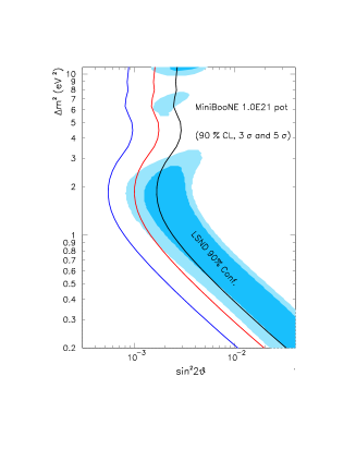
Figure 12: The region of oscillation parameters selected by LSND result versus sensitivity of the MiniBooNE experiment; from miniboone .

Of course, confirmation of the LSND result (in terms of oscillations) would be the most decisive though the problem with background should be scrutinized. The negative result still may leave an ambiguous situation. In fig. 12 the sensitivity limits and discovery potential of MiniBooNE are shown.

VI Conclusion

After the first phase of studies of neutrino mass and mixing we have rather consistent picture: interpretation of all the results (except for LSND) in terms of vacuum mixing of three massive neutrinos. Two main effects (consequences of mixing) are important for the interpretation of results at the present level of accuracy: the vacuum oscillations and the adiabatic conversion in matter (the MSW-effect). The oscillations in matter give sub-leading contributions, at $(1-2)\sigma$ level, to the solar and atmospheric neutrino observables.

There are unknown yet parameters and their determination composes a program of future phenomenological and experimental studies. Next phase of the field, study of sub-leading effects, will be much more involved.

The main theoretical challenge is to understand what is behind the observed pattern of neutrino masses and mixing (as well as masses and mixings of other fermions). What is the underlying physics? Clearly there is a strong difference of the quark and lepton mixing patterns. The data hint the tri-bimaximal scheme of mixing with possible implications of new “neutrino symmetries”, or alternatively to the quark-lepton complementarity that hints certain quark-lepton symmetry and unification. Are the tri-bimaximal or QLC relations real (follow from certain principles) or simply accidental?

It may happen that something important in principles and context is still missed. The key question is how far we can go in this understanding using our usual notions of the field theory (or the effective field theory) and in terms of symmetries, various mechanisms of symmetry breaking, etc.? The hope is that neutrinos will uncover something simple and illuminating before we will be lost in the string landscape.

References

- (1) B. Pontecorvo, Zh. Eksp. Theor. Fiz. 33 (1957); ibidem 34 (1958) 247.
- (2) Z. Maki, M. Nakagawa and S. Sakata, Prog. Theor. Phys. 28 (1962) 870.
- (3) B. Pontecorvo, ZETF, 53, 1771 (1967) [Sov. Phys. JETP, 26, 984 (1968)]; V. N. Gribov and B. Pontecorvo, Phys. Lett. 28B (1969) 493.
- (4) L. Wolfenstein, Phys. Rev. D17 (1978) 2369; in “Neutrino -78”, Purdue Univ. C3, (1978), Phys. Rev. D20 (1979) 2634.
- (5) S. P. Mikheyev and A. Yu. Smirnov, Sov. J. Nucl. Phys. 42 (1985) 913; Nuovo Cim. C9 (1986) 17; S.P. Mikheev and A.Yu. Smirnov, Sov. Phys. JETP 64 (1986) 4.
- (6) A.Yu. Smirnov and G.T. Zatsepin, Mod. Phys. Lett. A7 (1992) 1272.
- (7) N. Cabibbo, Summary talk given at 10th Int. Workshop on Weak Interactions and Neutrinos, Savonlinna, Finland, June 1985.
- (8) H. Bethe, Phys. Rev. Lett. 56 (1986) 1305.
- (9) P. Q. Hung, hep-ph/0010126; Peihong Gu, Xiulian Wang, Xinmin Zhang, Phys.Rev. D68, 087301 (2003); R. Fardon, A. E. Nelson, N. Weiner, JCAP 0410 005 (2004); hep-ph/0507235; D. B. Kaplan, A. E. Nelson, N. Weiner, Phys. Rev. Lett. 93, 091801 (2004); P. Q. Hung and H. Pas, Mod. Phys. Lett. A 20, 1209 (2005); A. Brookfield, C. van de Bruck, D.F. Mota, D. Tocchini-Valentini, Phys. Rev. Lett. 96, 061301 (2006).
- (10) A. Messiah, Proc. of the 6th Moriond Workshop on Massive Neutrinos in Particle Physics and Astrophysics, eds O. Fackler and J. Tran Thanh Van, Tignes, France, Jan. 1986, p. 373; S. P. Mikheev and A. Y. Smirnov, Sov. Phys. JETP 65, 230 (1987).
- (11) S. J. Parke, Phys. Rev. Lett. 57 (1986) 1275.
- (12) W. C. Haxton, Phys. Rev. Lett. 57 (1986) 1271.
- (13) P. C. de Holanda, Wei Liao, A. Yu. Smirnov, Nucl. Phys. B702 (2004) 307.
- (14) B. T. Cleveland et al., Astrophys. J. 496 (1998) 505.
- (15) J. Hosaka et al. [Super-Kamkiokande Collaboration], arXiv:hep-ex/0508053.
- (16) J. N. Abdurashitov et al. [SAGE Collaboration], J. Exp. Theor. Phys. 95 (2002) 181 [Zh. Eksp. Teor. Fiz. 122 (2002) 211].
- (17) W. Hampel et al. [GALLEX Collaboration], Phys. Lett. B 447 (1999) 127.
- (18) M. Altmann et al. [GNO COLLABORATION Collaboration], Phys. Lett. B 616 (2005) 174.
- (19) SNO Collaboration (B. Aharmim et al.). Phys. Rev. C 72 (2005) 055502; see also [SNO Collaboration] arXiv:nucl-ex/0610020.
- (20) J. N. Bahcall, M.H. Pinsonneault, Phys. Rev. Lett. 92 (2004) 121301; J. N. Bahcall, A. M. Serenelli and S. Basu, astro-ph/0511337.
- (21) P. C. de Holanda, A.Yu. Smirnov, Astropart. Phys. 21 (2004) 287.
- (22) A. N. Ioannisian and A.Yu. Smirnov, Phys. Rev. Lett. 93 (2004) 241801.
- (23) E. K. Akhmedov, M. A. Tortola and J. W. F. Valle, JHEP 0405 (2004) 057.
- (24) See e.g. B. Aharmim et al. [SNO Collaboration], Phys. Rev. D 72 (2005) 052010.
- (25) L. Miramonti [BOREXINO Collaboration], arXiv:hep-ex/0609011.
- (26) J.N. Abdurashitov et al., Prepared for 11th International Workshop on Neutrino Telescopes, Venice, Italy, 22-25 Feb 2005. In *Venice 2005, Neutrino telescopes* p. 187.
- (27) G. L. Fogli, E. Lisi, A. Marrone and A. Palazzo, arXiv:hep-ph/0605186.
- (28) C. Giunti and M. Laveder, arXiv:hep-ph/0610352.
- (29) T. Araki et al. [KamLAND Collaboration], Phys. Rev. Lett. 94 (2005) 081801.
- (30) A. Suzuki, Prepared for 3rd International Workshop on NO-VE: Neutrino Oscillations in Venice: 50 Years after the Neutrino Experimental Discovery, Venice, Italy, 7-10 Feb 2006.
- (31) Super-Kamiokande Collaboration (Y. Ashie et al.), Phys. Rev. D 71 (2005) 112005.
- (32) K. Abe et al. [Super-Kamiokande Collaboration], Phys. Rev. Lett. 97 (2006) 171801.
- (33) M. Ambrosio et al. [MACRO Collaboration], Eur. Phys. J. C 36 (2004) 323.
- (34) M. C. Sanchez et al. [Soudan 2 Collaboration], Phys. Rev. D 68 (2003) 113004.
- (35) [MINOS Collaboration], arXiv:hep-ex/0512036. P. Adamson [MINOS Collaboration], arXiv:hep-ex/0701045.
- (36) Y. Ashie et al. [Super-Kamiokande Collaboration], Phys. Rev. Lett. 93 (2004) 101801.
- (37) M. C. Gonzalez-Garcia, M. Maltoni, A. Yu. Smirnov, Phys. Rev. D 70 (2004) 093005.
- (38) G. L. Fogli, E. Lisi, A. Marrone and A. Palazzo, Prog. Part. Nucl. Phys. 57 (2006) 742, [hep-ph/0506083].
- (39) E. Aliu et al. [K2K Collaboration], Phys. Rev. Lett. 94 (2005) 081802.
- (40) D. G. Michael et al. [MINOS Collaboration], Phys. Rev. Lett. 97 (2006) 191801
- (41) M. Apollonio et al., Eur. Phys. J. C 27 (2003) 331.
- (42) A. Strumia, F. Vissani, Nucl. Phys. B 726 (2005) 294.
- (43) M. Maltoni, T. Schwetz, M. A. Tortola and J. W. F. Valle, New J. Phys. 6 (2004) 122, [arXiv:hep-ph/0405172] v.6 (2006).
- (44) L. Wolfenstein, Phys. Rev. D 18, 958 (1978); P. F. Harrison, D. H. Perkins and W. G. Scott, Phys. Lett. B 458, 79 (1999), Phys. Lett. B 530, 167 (2002).
- (45) A. Yu. Smirnov, hep-ph/0402264; M. Raidal, Phys. Rev. Lett. 93 (2004) 161801; H. Minakata, A. Yu. Smirnov, Phys. Rev. D 70 (2004) 073009.
- (46) M. A. Schmidt and A. Y. Smirnov, Phys. Rev. D 74 (2006) 113003 [arXiv:hep-ph/0607232].
- (47) V. M. Lobashev et al., Nucl. Phys. Proc. Suppl. 91 (2001) 280.
- (48) C. Kraus et al., Eur. Phys. J. C 40 (2005) 447.
- (49) A. Osipowicz et al. [KATRIN Collaboration], arXiv:hep-ex/0109033.
- (50) H.V. Klapdor-Kleingrothaus et al., Eur. Phys. J. A 12, 147 (2001); A. M. Bakalyarov et al., talk given at the 4th International Conference on Non-accelerator New Physics (NANP 03), Dubna, Russia, 23-28 Jun. 2003, hep-ex/0309016.
- (51) H.V. Klapdor-Kleingrothaus et al., Mod. Phys. Lett. A 16 (2001) 2409.
- (52) H.V. Klapdor-Kleingrothaus, et al, Phys. Lett. B 586 (2004) 198.
- (53) C. E. Aalseth et al. [IGEX Collaboration], Phys. Rev. D65 092007 (2002); C. E. Aalseth et al., Phys. Rev. D 70 (2004) 078302.
- (54) R. Arnold et al. [NEMO Collaboration], Phys. Rev. Lett. 95 (2005) 182302.
- (55) P. Gorla et al., Prepared for 2nd Scandanavian Neutrino Workshop (SNOW 2006), Stockholm, Sweden, 2-6 May 2006. Phys. Scripta 127, 49 (2006).
- (56) GERDA Collaboration (E. Bellotti for the collaboration). Prepared for 9th International Conference on Astroparticle and Underground Physics (TAUP 2005), Zaragoza, Spain, 10-14 Sep 2005. J. Phys.Conf.Ser. 39, 338 (2006).
- (57) U. Seljak et al.. Phys. Rev. D 71 (2005) 103515.
- (58) A. Goobar, S. Hannestad, E. Mortsell and H. Tu, astro-ph/0602155.
- (59) U. Seljak, A. Slosar and P. McDonald, arXiv:astro-ph/0604335.
- (60) Y. Itow et al., hep-ex/0106019.
- (61) D. S. Ayres et al. [NOvA Collaboration], hep-ex/0503053.
- (62) F. Ardellier et al., “Letter of intent for double-CHOOZ”, hep-ex/0405032.
- (63) X. Guo [Daya Bay Collaboration], arXiv:hep-ex/0701029; Y. f. Wang, arXiv:hep-ex/0610024.
- (64) A. S. Dighe, A. Yu. Smirnov, Phys. Rev. D62, 033007 (2000); C. Lunardini, A. Yu. Smirnov, JCAP 0306, 009 (2003).
- (65) H. Minakata, H. Nunokawa, Phys. Lett. B 504 (2001) 301.
- (66) V. Barger, D. Marfatia, B.P. Wood, Phys. Lett. B 532 (2002) 19.
- (67) K. Takahashi, K. Sato, A. Burrows, T. A. Thompson, Phys. Rev. D 68 (2003) 113009.
- (68) J. T. Pantaleone, Phys. Lett. B 287 (1992) 128; J. T. Pantaleone, Phys. Lett. B342, 250 (1995); for recent discussion and references see, e.g., A. Friedland and C. Lunardini, Phys.Rev. D68, 013007 (2003); R. F. Sawyer, Phys. Rev. D 72 (2005) 045003; G. M. Fuller and Y. Z. Qian, Phys. Rev. D 73 (2006) 023004; S. Hannestad, G. G. Raffelt, G. Sigl and Y. Y. Y. Wong, Phys. Rev. D 74 (2006) 105010.
- (69) R.C. Schirato and G. M. Fuller, astro-ph/0205390.
- (70) K. Takahashi, K. Sato, H. E. Dalhed, J.R. Wilson, Astropart. Phys. 20, 189 (2003).
- (71) G.L. Fogli, E. Lisi, D. Montanino, A. Mirizzi, Phys. Rev. D 68, 033005 (2003).
- (72) R. Tomas, et al., JCAP 0409 (2004) 015.
- (73) A. Aguilar et al., (LSND Collaboration) Phys. Rev. D 64 (2001) 112007.
- (74) B. Armbruster, et al., (KARMEN), Phys. Rev. Lett., 90, 181804 (2003).
- (75) K. S. Babu and S. Pakwasa, hep-ph/0204226.
- (76) G. Barenboim, L. Borissov, J. Lykken, hep-ph/0212116.
- (77) A. Strumia, Phys. Lett. B 539, 91 (2002).
- (78) M.C. Gonzalez-Garcia, M. Maltoni T. Schwetz, Phys. Rev. D 68, 053007 (2003).
- (79) O. L. G. Peres, A.Yu. Smirnov, Nucl. Phys. B 599 (2001) 3.
- (80) M. Sorel, J. Conrad, M. Shaevitz, Phys. Rev. D 70 (2004) 073004.
- (81) V. Barger, D. Marfatia, K. Whisnant, Phys. Lett. B 576 (2003) 303.
- (82) S. Palomares-Ruiz, S. Pascoli and T. Schwetz, JHEP 0509 (2005) 048.
- (83) M. H. Shaevitz [MiniBooNE Collaboration], Nucl. Phys. Proc. Suppl. 137 (2004) 46.