Axions, their Relatives and Prospects for the Future

Abstract

The observation of a non-vanishing rotation of linear polarized laser light after passage through a strong magnetic field by the PVLAS collaboration has renewed the interest in light particles coupled to photons. Axions are a species of such particles that is theoretically well motivated. However, the relation between coupling and mass predicted by standard axion models conflicts with the PVLAS observation. Moreover, light particles with a coupling to photons of the strength required to explain PVLAS face trouble from astrophysical bounds. We discuss models that can avoid these bounds. Finally, we present some ideas to test these possible explanations of PVLAS experimentally.

IPPP/07/03
                                                                                                                    DCPT/07/06

1 Motivation – the PVLAS Observation

Recently, the PVLAS collaboration reported the observation of a non-vanishing rotation of linear polarized laser light after passage through a strong transverse magnetic field [1],

$$\Delta\theta\sim 10^{-12}\,\rm{rad}$$ (1)

per pass through a magnetic field of $B\approx 5\,\rm{T}$ and length $L=1\,\rm{m}$ and using a laser with wavelength $\lambda\sim 1000\,\rm{nm}$. Such a signal is not expected in standard QED with electrons. If confirmed this could be the first direct evidence for physics beyond the standard model.

One obvious possible explanation, and indeed the one which was also a motivation for the BFRT [2, 3] and PVLAS experiments, may be offered by the existence of a new light neutral spin-$0$ boson $\phi$ [4] that could be a scalar or a pseudoscalar. If this particle is, e.g., a pseudoscalar the interaction reads

$${\mathcal{L}}_{\rm{int}}=-\frac{1}{4}g\phi F_{\mu\nu}\widetilde{F}^{\mu\nu}=g\phi(\vec{E}\cdot\vec{B}).$$ (2)

In a homogeneous magnetic background $\vec{B}$, this interaction can convert the laser photons into pseudoscalars (upper part of Fig. 1). The leading order contribution to this process comes from the term $\sim\vec{E}_{\gamma}\cdot\vec{B}$. The polarization of a photon is given by the direction of the electric field of the photon, $\vec{E}_{\gamma}$. Therefore, only those fields polarized parallel to the background magnetic field will have nonvanishing $\vec{E}_{\gamma}\cdot\vec{B}\neq 0$ and interact with the pseudoscalar particles. As depicted in Fig. 1 this leads to an absorption of photons with a polarization parallel to the magnetic field and this in turn leads to an overall rotation of the polarization.

The rotation observed by PVLAS can be reconciled with the non-observation of a rotation and ellipticity by the earlier BFRT experiment [2, 3], if the hypothetical neutral boson has a mass and a coupling to two photons in the range

$$m_{\phi}\sim(1-1.5)\,\rm{meV}\quad\quad g\sim(1.7-5.0)\times 10^{-6}\,\rm{GeV}^{-1}.$$ (3)

In addition to the rotation preliminary data [6, 7] presented at various conferences suggests the existence of a small ellipticity,

$$\psi\sim 10^{-12}\,\rm{rad}$$ (4)

per pass through the magnetic field (parameters as above). Such a signal could be explained by the virtual production of particles as depicted in the lower part of Fig. 1. Again, only the photons polarized parallel to the magnetic field are affected. Roughly speaking those are a bit delayed because the massive intermediate particle is a bit slower. This results in a phase difference between the polarizations parallel and perpendicular to the magnetic field which appears as an ellipticity in the final polarization. This allows an independent calculation of the required mass $m_{\phi}$ using only PVLAS data. The results are consistent with Eq. (3) [8].

Figure 1: Rotation (upper half) and ellipticity (lower half) caused by the existence of a light neutral spin-0 boson (left) or a light particle with a small electric charge (right) (figure adapted from [5]).

An alternative [9] is the existence of light particles with a small electric charge. These are often called millicharged particles although their charge may be significantly less than $10^{-3}$. They could be bosons or fermions. For example, for fermions the interaction part of the Lagrangian would be

$${\mathcal{L}}_{\rm int}^{\rm Dsp}=\epsilon\,e\,\overline{\psi}_{\epsilon}\gamma_{\mu}\psi_{\epsilon}A^{\mu},$$ (5)

with $\psi_{\epsilon}$ being a Dirac spinor (“Dsp”). As depicted in Fig. 1 the explanation of a possible rotation and ellipticity signal works in complete analogy to the case of spin-0 particles only pairproduction now replaces single particle production. Although it is not immediately obvious from the interaction Lagrangian, the rate for pairproduction and the birefringence caused by virtual pairproduction do again depend on the relative orientation of laser polarization and background magnetic field [10, 11, 12, 13, 14, 15, 16, 17].

It is clear that millicharged particles, too, must be light to allow for the rotation observed in PVLAS. Real production of pairs requires that the total mass of the produced particles is less than the energy of the laser photon $2m_{\epsilon}\leq\omega_{\gamma}$ since the (constant) background field cannot contribute to the energy. Furthermore the charge must be sufficiently small to avoid conflicts with other existing laboratory experiments $\epsilon\lesssim 10^{-5}$ [18, 19, 20, 21]. Consistency with PVLAS, BFRT and the recent Q&A measurements [22] requires [8, 9],

$$m_{\epsilon}\lesssim 0.1\,\rm{eV}\quad\quad\epsilon\sim 10^{-6}.$$ (6)

2 Axions in a Nutshell

One light particle species coupled to photons is particularly well motivated by theory: axions [23, 24, 25, 26]. Therefore, let us briefly review axions and discuss their (in)viability to explain PVLAS (for a more complete review of axions see, e.g., [27, 28]).

Axions are motivated by the so called strong CP problem. As the name indicates it has its origin in the theory of strong interactions, QCD. Therefore, let us start by writing down the Lagrangian of QCD with quarks,

$$S=\int d^{4}x\bigg{[}-\frac{1}{4g^{2}}G^{a,\mu\nu}G^{a}_{\mu\nu}-\frac{\theta}{32\pi^{2}}G^{a,\mu\nu}\tilde{G}^{a}_{\mu\nu}+\i\bar{\psi}D_{\mu}\gamma^{\mu}\psi+\bar{\psi}{\rm{M}}\psi\bigg{]},$$ (7)

where $G$ is the gluon field strength and $\tilde{G}$ its dual. This Lagrangian contains a term $\sim\theta G\tilde{G}$ that is often absent in discussions of QCD. This term is perfectly allowed by gauge symmetry. So why is it often neglected? The reason is that this term violates CP in a strong manner but this is not observed in nature. More precisely,

$$\theta+\rm{Arg}\det(M)\quad\rm{is~{}observable}$$ (8)

and would appear in CP violating properties of hadrons as, e.g., an electric dipole moment of the neutron. Measurements of the electric dipole moment of the neutron [29, 30] now constrain

$$|\theta+\rm{Arg}\det(M)=0|<3\times 10^{-10}.$$ (9)

As mentioned in the beginning of this section $\theta$ is an allowed parameter which is undetermined in QCD. Naturally it should be of order one. So the question is: why is it so small? This naturalness problem is the strong CP problem.

One prominent mechanism to solve this problem is the axion solution. The idea is to make $\theta$ a dynamical degree of freedom with the following properties:

• $\theta$ has no tree-level potential

• $\theta$ has only derivative couplings.

Choosing a basis such that $\rm{Arg}\det(M)=0$ one can then show (see, e.g., [27]) that for the effective potential,

$$V[0]<V[\theta],$$ (10)

i.e. the global minimum of the potential lies at the CP conserving value $\theta=0$, and $\theta$ will automatically evolve towards this value.

However, there is still the question from where this dynamical degree of freedom originates. Using

$$\int d^{4}x\frac{G^{a,\mu\nu}\tilde{G}^{a}_{\mu\nu}}{32\pi^{2}}=n\in{\mathbb{Z}}$$ (11)

one finds that $\theta$ is an angular degree of freedom

• $\theta\in[0,2\pi)$.

Together with the two above properties this is reminiscent of a Goldstone boson of a spontaneously broken U(1) symmetry. Choosing a suitable axial U(1) symmetry one finds indeed that for the Goldstone direction a coupling to $G\tilde{G}$ is generated via a triangle diagram. This is the famous Peccei-Quinn symmetry [25, 26] and the particle is the axion [23, 24].

So far we have been talking about the axion as a Goldstone boson. However, Eq. (10) already shows that the potential for the axion is not completely flat and the particle will have an effective mass. Indeed, the Peccei-Quinn symmetry is anomalous and the axion is only a pseudo-Goldstone boson.

A simple estimate (for more see, e.g., [23, 35, 36, 37]) for this mass can be obtained by looking at the transformations of the up and down quark condensates under chiral rotations $\alpha$ and Peccei-Quinn rotations $\sim\theta$,

$$\langle\bar{u}_{\rm{L}}u_{\rm{R}}\rangle=|\langle\bar{u}_{\rm{L}}u_{\rm{R}}\rangle|\exp(\i(\alpha+c_{u}\theta))\quad{\rm{and}}\quad\langle\bar{d}_{\rm{L}}d_{\rm{R}}\rangle=|\langle\bar{d}_{\rm{L}}d_{\rm{R}}\rangle|\exp(\i(-\alpha+c_{d}\theta)),$$ (12)

where $c_{u}$ and $c_{d}$ are constants. Taking the expectation value of the quark mass terms in the Lagrangian and approximating $\langle\bar{u}u\rangle\approx\langle\bar{u}u\rangle$ one finds a contribution to the effective potential,

$$V\sim|\langle\bar{u}u\rangle|\left[m_{u}\cos(\alpha+c_{u}\theta)+m_{d}\cos(\alpha-c_{d}\theta)\right],$$ (13)

with the up and down quark masses $m_{u}$ and $m_{d}$. Expanding to second order in the fields and using properly normalized pion, $\pi_{0}$, and axion, $a$, fields,

$$\alpha=\frac{\pi_{0}}{f_{\pi}},\quad\theta=\frac{a}{f_{a}}$$ (14)

one finds

$$f^{2}_{\pi}m^{2}_{\pi}=(m_{u}+m_{d})\langle\bar{u}u\rangle$$ (15)

and

$$m^{2}_{a}\sim\frac{f^{2}_{\pi}m^{2}_{\pi}}{f^{2}_{a}}.$$ (16)

Here, $f_{\pi}$ is the pion decay constant and $f_{a}$ is the axion decay constant which characterize the scale of (spontaneous) chiral and Peccei-Quinn symmetry breaking, respectively.

The, for our purposes particularly important, coupling to the electromagnetic field strength arises via a similar triangle diagram as the coupling to the gluonic field strength. Naturally it involves the elctromagnetic coupling $\alpha$,

$${\rm{coupling~{}to~{}two~{}photons}}\sim\alpha\frac{a}{f_{a}}F^{\mu\nu}\tilde{F}_{\mu\nu}.$$ (17)

Please note that $f_{\pi}$ and $m_{\pi}$ are known and we have only one free parameter, $f_{a}$, in Eqs. (16) and (17). Mass and coupling of the axion are related. Therefore, axions are confined to a line in the mass-coupling plane. Of course our analysis neglected model dependent factors of order unity and the line becomes a (narrow) band as shown in Fig. 2.

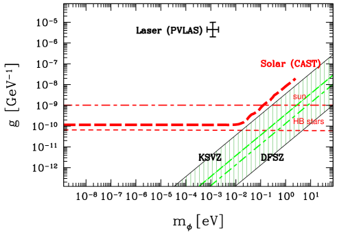
Figure 2: Mass-coupling plane for axion-like particles. The cross denotes the coupling required to explain PVLAS. The green shaded area gives the typical range allowed for true axions and the green lines denote two prominent examples of axion models [31, 32, 33, 34]. The red lines represent the bounds from astrophysics (everything above the lines is excluded). The bounds labelled “sun” and “HB stars” come from energy loss considerations [38, 39, 40, 41], the “CAST” bound comes from the non-observation of axion-like particles in the CAST experiment that aims to reconvert ALPs generated in the sun into photons [42].

As we can see from Fig. 2 the mass and coupling required to explain the PVLAS observation is orders of magnitude outside the range allowed for axion models. Therefore, we cannot use the true axions invented to solve the strong CP problem to explain PVLAS. In the following we will call light particles coupled to two photons but without the mass-coupling relation axion-like particle or ALPs.

3 Astrophysical Bounds

A serious challenge for the particle interpretation of PVLAS are the extremely tight bounds on the couplings of light particles to photons. In this section we will sketch how those bounds arise and in the following Sect. 4 we discuss some ideas from the recent literature to circumvent them.

3.1 Energy loss bound

The production processes depicted in the upper half of Figs. 1 can also occur in the plasma in the central regions of the sun. Photons of the solar plasma interact with the electromagnetic fields provided by the ions and electrons in the plasma and are converted into ALPs. If the coupling of these particles is, however, sufficiently small they immediately leave the sun without further scattering – each one carrying away an energy of the order of $T_{\rm{center}}\sim 10^{7}\,\rm{K}\sim 1\,\rm{keV}$. This is in stark contrast to photons. Photons typically scatter millions and millions of times until they reach the surface of the sun. This has two effects. First it simply takes longer for a photon to leave the sun, slowing down the energy transport via photons. Second on their long way to the surface the photons loose energy and stay thermalized. They leave the sun only with energies of the order of the surface temperature $T_{\rm{surface}}\sim 6000\,\rm{K}\sim 1\,\rm{eV}$ instead of having energies typical for the center of the sun $\sim 1\,\rm{keV}$ resulting in a further slowdown of the energy transport.

Overall this makes the energy loss channel via light particles weakly coupled to photons extremely efficient when compared to the standard one via photons. For example, for ALPs one finds [41]

$$L_{\rm{ALP}}\sim 10^{7}\left(g\,10^{5}\rm{GeV}\right)^{2}L_{\gamma},$$ (18)

where $L_{\rm{ALP}}$ is the energy loss via ALPs and $L_{\gamma}$ the one via photons.

To compensate for the additional energy loss channels the sun would have to burn fuel at a much faster rate. Without additional light particles the sun has enough nuclear fuel for about $10^{10}\,\rm{years}$. Using Eq. (18) we can easily estimate that in the presence of ALPs with a coupling strong enough to explain PVLAS the sun would have fuel for at most a few 1000 years. Clearly in conflict with observation. A more detailed analysis strengthens the bound to the limit [38, 41] depicted in Fig. 2. Including data from so called horizontal branch (HB) stars one can improve it even more [39, 40] (cf. Fig. 2).

For millicharged particles the production process in the upper half of Fig. 1 can be used for a similar argument leading to [43, 44, 45, 46, 47],

$$\epsilon\lesssim 10^{-14}\quad\rm{for}\quad m_{\epsilon}\lesssim 1\,\rm{keV}.$$ (19)

3.2 CAST Bound

For ALPs one can also try to reconvert the ALPs generated in the sun [48]. Basically this uses the inverse of the production process of Fig. 1. The CAST collaboration [42] has set up such an experiment using an LHC test magnet to provide the background magnetic field. Looking in the direction of the sun one would expect to regenerate photons with energies of a few $\rm{keV}$ (temperature of the sun). So far CAST has found no signal above the background. This gives the “CAST” bound in Fig. 2.

For millicharged particles the CAST idea does not work because it is highly unlikely that two millicharged particles would meet again inside the CAST magnet.

4 Evading Astrophysical Bounds

Inspired by the PVLAS result and the apparent conflict with astrophysical bounds several models to evade the astrophysical bounds have been proposed. We will start by discussing a few ideas that apply to ALPs then we move briefly to millicharged particles until we come to a few entirely different ideas to explain PVLAS without violating astrophysical bounds.

4.1 Trapping

One central property that leads to the tightness of astrophysical bounds is the fact that ALPs, once produced, immediately leave the sun. So one might want to endow the ALPs with some additional interaction that prevents their escape from the sun basically trapping them in the sun (at least for some time). This would dramatically reduce the energy loss. Moreover, it would also prevent detection via CAST because the ALPs would loose energy in scattering processes making them undetectable by CAST which is sensitive only to ALPs with energies $\gtrsim 1\,\rm{keV}$. The basic concept for this mechanism was already sketched in [49] and models were presented in [50, 51].

This idea has one essential difficulty. To achieve a sufficient amount of scattering of ALPs within the sun one needs a fairly large interaction making it difficult to avoid detection in other experiments and observations. However, so far no such conflicts have been found for the models [50, 51] and they remain viable.

4.2 Suppressed Production

An alternative to trapping is to find a way to suppress the production of ALP’s inside the sun. Models of this type are based on the fact that the environment inside the sun is different from the lab environment of PVLAS. The various proposed models make use of different parameters that are higher in the sun than in the lab:

• The typical virtuality of the process producing the ALPs [49, 52]

• The plasma frequency in the solar plasma [49, 52]

• Temperature [53]

• Density [54].

The problem with these models is that they typically involve at least one unnaturally small parameter. This difficulty is enhanced by the fact that it is not enough to suppress the production of ALPs in the center of the sun but one has to achieve suppression also in the outer parts of the sun where temperature, density etc. are significantly smaller than in the center [54].

4.3 Millicharged Particles

As we already discussed pair production of millicharged particles can provide an alternative [9] to the single production of neutral particles coupled to two photons. However, we already saw in Sect. 3 that they face similar problems from astrophysical bounds. The most straightforward way to avoid this problem is, again, to switch off production. Indeed the model [52] already involves millicharged fermions and is actually simplified by removing the additional axion-like particle.

A nice feature of this model is that millicharged particles occur naturally in extensions of the standard model [55, 56, 57]. For example, in D-brane models of string theory one can find the right representations and a sufficient amount of kinetic mixing to explain PVLAS [58]. Nevertheless, there remains an unexplained small mass scale of the order of $\rm{meV}$ in these models, too.

4.4 Other proposals

In addition to the above there have been a few proposals that involve neither spin-0 bosons coupled to two photons nor millicharged particles.

One possibility is spacetime noncommutativity [59]. This idea avoids additional light particles and therefore also their problems with astrophysical bounds. However, a recent careful study [60] suggests that spacetime noncommutativity produces only an ellipticity and cannot explain the rotation signal of PVLAS.

Another possibility tried to employ an additional vector particle [61]. This also produces an ellipticity but, unfortunately, probably fails to produce the required amount of rotation.

Finally, there has been a claim [62] that the PVLAS result can be explained within standard QED if the (slow) rotation of the background magnetic field is taken into account. A careful wave-propagation study [63, 64] has, however, shown that this is ruled out.

5 Experimental Tests

Confirmation of the PVLAS result and distinguishing between the different proposed models requires further experiments. One way is to make an independent experiment testing and improving the measurements of PVLAS. One experiment currently under way is the Q&A experiment which recently has published first data [22] but more data from different sources is expected in the near future [65, 66, 67]. A detailed analysis of the data from such optical experiments may even allow to distinguish between axion-like and millicharged particles [8].

However, an experiment of the PVLAS type is a disappearance experiment (the produced particles are not detected). It would be nice to really have some way to actually detect the proposed particles. In this section we want to sketch two experiments that are sensitive to axion-like particles and millicharged particles, respectively.

5.1 Light Shining through Walls

To test for the existence of spin-0 bosons coupled to two photons one can do a so called “light shining through a wall experiment” [68, 69, 70, 71] as sketched in Fig. 3. Here, the photons are first converted into ALPs using a strong magnetic field. Then the photon beam is stopped by a thick wall. The weakly interacting ALPs, however, pass through this wall without any problems. Behind the wall another magnetic field is used to reconvert the ALPs into photons via the inverse production process. The photons (coming “out of the wall”) are then detected. This is a very clean detection experiment. The photons coming out of the wall have the same frequency as the laser making it easier to distinguish them from the background. Moreover the number of photons coming out of the wall is directly correlated to the strength of the laser, e.g. for a pulsed laser one can then use the resulting time dependence of the signal to further improve the signal/noise ratio.

Figure 3: Schematic view of a “light shining through a wall” experiment. (Pseudo-)scalar production through photon conversion in a magnetic field (left), subsequent travel through a wall, and final detection through photon regeneration (right).

Currently, at least four such experiments are in advanced planning/testing stages (for a recent review see [72]). One at DESY [73], one at Jefferson lab [74], one by the BMV collaboration [66] and one at CERN [65]. The PVLAS collaboration themselves also plan an extension of their experiment [75].

5.2 Dark Currents Shining through a Wall

Unfortunately, a light shining through a wall experiments will not work for millicharged particles. Once produced the particle and the antiparticle will move away from each other since they experience opposite forces in the magnetic field due to their opposite charges. They will simply not meet again behind the wall and reconversion does not occur (most of them will not even make it to the wall because the magnetic field forces them on circular trajectories).

A way out is to use another QED process: Schwinger pair production [76]. In a strong electric field (without an additional laser) vacuum pairs of charged particles that are created at a sufficiently large distance,

$$d>d_{\rm{pair}}=\frac{2m_{\epsilon}}{\epsilon e\mathbf{E}}$$ (20)

have gained more energy from the electric field than it cost to produce them and it is energetically favorable to produce such pairs. Roughly speaking this is a tunneling process where a barrier of height $2m_{\epsilon}$ (the energy to produce the pair) and width $d_{\rm{pair}}$ (the distance needed to gain enough energy in the electric field) must be overcome. The pairproduction rate is high if the electric field is large enough such that $d_{\rm{pair}}/2$ is smaller than the Compton wavelength of the particles $\lambda_{C}=1/m_{\epsilon}$,

$$\mathbf{E}>\mathbf{E}_{\rm{crit}}=\frac{m^{2}_{\epsilon}}{\epsilon e}.$$ (21)

Since the produced particles typically have momenta along the lines of the electric field for the positive charge particle and in the opposite direction for the negative counterpart a current is generated. This current can be measured with a setup shown in Fig. 4. Using existing accelerator cavities as source of the electric field such an experiment could be build in the near future allowing to test the millicharged particle interpretation of PVLAS [77].

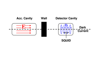
Figure 4: Schematic set up for a “dark current shining through a wall” experiment [77]. The alternating dark current (frequency $\nu$), comprised of the produced millicharged particles (dashed line), escapes from the accelerator cavity and traverses also a thick shielding (“wall”), in which the conventional dark current of electrons is stopped. The dark current induces a magnetic field in a resonant (frequency $\nu$) detector cavity behind the wall, which is detected by a SQUID.

6 Conclusions

Motivated by the surprising observation of a non-vanishing rotation of linear polarized laser light in a magnetic field by the PVLAS collaboration we have reviewed light particles coupled to photons.

While standard QCD axions are unable to explain PVLAS similar light particles coupled to two photons, axion-like particles, may do so. Another candidate are light particles with a small electric charge. If confirmed the PVLAS signal would be the first direct evidence for physics beyond the standard model.

Both particle interpretations of PVLAS face serious problems from astrophysical bounds (so far other explanation attempts have not been succesful). Models to avoid the astrophysical bounds can be constructed but typically require some fine-tuning.

Several experiments to test PVLAS and its particle interpretations are currently under way or will/can be build in the near future.

The existence of light particles coupled to photons would open a window to physics beyond the standard model via low energy experiments with photons that is complementary to conventional accelerator experiments.

Bibliography

Bibliography

- [1] E. Zavattini et al. [PVLAS Collaboration], Phys. Rev. Lett. 96, 110406 (2006) [hep-ex/0507107].
- [2] Y. Semertzidis et al. [BFRT Collaboration], Phys. Rev. Lett. 64, 2988 (1990).
- [3] R. Cameron et al. [BFRT Collaboration], Phys. Rev. D 47, 3707 (1993).
- [4] L. Maiani, R. Petronzio and E. Zavattini, Phys. Lett. B 175, 359 (1986).
- [5] F. Brandi et al., Nucl. Instrum. Meth. A 461 (2001) 329 [hep-ex/0006015].
-
[6]
U. Gastaldi, on behalf of the PVLAS Collaboration, talk at ICHEP‘06, Moscow,
http://ichep06.jinr.ru/reports/42_1s2_13p10_gastaldi.ppt - [7] G. Cantatore for the PVLAS Collaboration, “Laser production of axion-like bosons: progress in the experimental studies at PVLAS,” talk presented at the 6th International Workshop on the Identification of Dark Matter (IDM 2006), Island of Rhodes, Greece, 11–16th September, 2006, http://elea.inp.demokritos.gr/idm2006_files/talks/Cantatore-PVLAS.pdf
- [8] M. Ahlers, H. Gies, J. Jaeckel and A. Ringwald, hep-ph/0612098.
- [9] H. Gies, J. Jaeckel and A. Ringwald, Phys. Rev. Lett. 97, 140402 (2006) [hep-ph/0607118].
- [10] J. S. Toll, Ph.D. thesis, Princeton Univ., 1952 (unpublished).
- [11] N. P. Klepikov, Zh. Eksp. Teor. Fiz. 26, 19 (1954).
- [12] T. Erber, Rev. Mod. Phys. 38, 626 (1966).
- [13] V. N. Baier and V. M. Katkov, Zh. Eksp. Teor. Fiz. 53, 1478 (1967) [Sov. Phys. JETP 26, 854 (1968)].
- [14] J. J. Klein, Rev. Mod. Phys. 40, 523 (1968).
- [15] S. L. Adler, Annals Phys. 67, 599 (1971).
- [16] W. y. Tsai and T. Erber, Phys. Rev. D 10, 492 (1974).
- [17] J. K. Daugherty and A. K. Harding, Astrophys. J. 273, 761 (1983).
- [18] T. Mitsui, R. Fujimoto, Y. Ishisaki, Y. Ueda, Y. Yamazaki, S. Asai and S. Orito, Phys. Rev. Lett. 70 (1993) 2265.
- [19] A. Badertscher et al., hep-ex/0609059.
- [20] A. A. Prinz et al., Phys. Rev. Lett. 81 (1998) 1175 [hep-ex/9804008].
- [21] S. N. Gninenko, N. V. Krasnikov and A. Rubbia, hep-ph/0612203.
- [22] S. J. Chen, H. H. Mei and W. T. Ni [Q& A Collaboration], hep-ex/0611050.
- [23] S. Weinberg, Phys. Rev. Lett. 40, 223 (1978).
- [24] F. Wilczek, Phys. Rev. Lett. 40, 279 (1978).
- [25] R. D. Peccei and H. R. Quinn, Phys. Rev. Lett. 38, 1440 (1977).
- [26] R. D. Peccei and H. R. Quinn, Phys. Rev. D 16, 1791 (1977).
- [27] J. E. Kim, Phys. Rept. 150 (1987) 1.
- [28] P. Svrcek and E. Witten, JHEP 0606 (2006) 051 [hep-th/0605206].
- [29] N. F. ,Ramsay Phys. Rept. 43 (1977) 409.
- [30] C. A. Baker et al., Phys. Rev. Lett. 97 (2006) 131801 [hep-ex/0602020].
- [31] J. E. Kim, Phys. Rev. Lett. 43 (1979) 103.
- [32] M. A. Shifman, A. I. Vainshtein and V. I. Zakharov, Nucl. Phys. B 166 (1980) 493.
- [33] M. Dine, W. Fischler and M. Srednicki, Phys. Lett. B 104 (1981) 199.
- [34] A. P. Zhitnitskii, Sov. J. Nucl. Phys. 31 (1980) 260.
- [35] M. Dine and W. Fischler Phys. Lett. B 120, 137 (1983).
- [36] P. Sikivie, Phys. Rev. Lett. 48, 1156 (1982).
- [37] S. Weinberg, The Quantum Theroy of Fields II, Cambridge University Press, Cambridge, 1996.
- [38] J. A. Frieman, S. Dimopoulos and M. S. Turner, Phys. Rev. D 36 (1987) 2201.
- [39] G. G. Raffelt, Phys. Rev. D 33 (1986) 897.
- [40] G. G. Raffelt and D. S. P. Dearborn, Phys. Rev. D 36 (1987) 2211.
- [41] G. G. Raffelt, Stars As Laboratories For Fundamental Physics: The Astrophysics of Neutrinos, Axions, and other Weakly Interacting Particles, University of Chicago Press, Chicago, 1996.
- [42] K. Zioutas et al. [CAST Collaboration], Phys. Rev. Lett. 94, 121301 (2005) [hep-ex/0411033].
- [43] S. Davidson, B. Campbell and D. C. Bailey, Phys. Rev. D 43 (1991) 2314.
- [44] R. N. Mohapatra and I. Z. Rothstein, Phys. Lett. B 247 (1990) 593.
- [45] R. N. Mohapatra and S. Nussinov, Int. J. Mod. Phys. A 7 (1992) 3817.
- [46] S. Davidson and M. E. Peskin, Phys. Rev. D 49 (1994) 2114 [hep-ph/9310288].
- [47] S. Davidson, S. Hannestad and G. Raffelt, JHEP 0005 (2000) 003 [hep-ph/0001179].
- [48] P. Sikivie, Phys. Rev. Lett. 51, 1415 (1983) [Erratum-ibid. 52, 695 (1984)].
- [49] E. Masso and J. Redondo, JCAP 0509, 015 (2005) [hep-ph/0504202].
- [50] P. Jain and S. Mandal, astro-ph/0512155.
- [51] P. Jain and S. Stokes, hep-ph/0611006.
- [52] E. Masso and J. Redondo, Phys. Rev. Lett. 97, 151802 (2006) [hep-ph/0606163].
- [53] R. N. Mohapatra and S. Nasri, hep-ph/0610068.
- [54] J. Jaeckel, E. Masso, J. Redondo, A. Ringwald and F. Takahashi, hep-ph/0605313; hep-ph/0610203.
- [55] B. Holdom, Phys. Lett. B 166, 196 (1986).
- [56] S. A. Abel and B. W. Schofield, Nucl. Phys. B 685 (2004) 150 [hep-th/0311051].
- [57] B. Batell and T. Gherghetta, Phys. Rev. D 73 (2006) 045016 [hep-ph/0512356].
- [58] S. A. Abel, J. Jaeckel, V. V. Khoze and A. Ringwald, hep-ph/0608248.
- [59] M. Chaichian, M. M. Sheikh-Jabbari and A. Tureanu, hep-ph/0511323.
- [60] N. Chatillon and A. Pinzul, Nucl. Phys. B 764 (2007) 95 [hep-ph/0607243].
- [61] I. Antoniadis, A. Boyarsky and O. Ruchayskiy, hep-ph/0606306.
- [62] J. T. Mendonca, J. Dias de Deus and P. Castelo Ferreira, Phys. Rev. Lett. 97, 100403 (2006) [hep-ph/0606099].
- [63] S. L. Adler, hep-ph/0611267.
- [64] S. Biswas and K. Melnikov, hep-ph/0611345.
- [65] P. Pugnat et al., Czech. J. Phys. 55, A389 (2005); Czech. J. Phys. 56, C193 (2006).
- [66] C. Rizzo [BMV Collaboration], 2nd ILIAS-CERN-CAST Axion Academic Training 2006, http://cast.mppmu.mpg.de/
- [67] T. Heinzl, B. Liesfeld, K. U. Amthor, H. Schwoerer, R. Sauerbrey and A. Wipf, hep-ph/0601076.
- [68] A. A. Anselm, Yad. Fiz. 42, 1480 (1985).
- [69] M. Gasperini, Phys. Rev. Lett. 59, 396 (1987).
- [70] K. Van Bibber, N. R. Dagdeviren, S. E. Koonin, A. Kerman and H. N. Nelson, Phys. Rev. Lett. 59, 759 (1987).
- [71] G. Ruoso et al. [BFRT Collaboration], Z. Phys. C 56, 505 (1992).
- [72] A. Ringwald, hep-ph/0612127.
- [73] K. Ehret et al. [ALPS Collaboration], LoI approved by DESY directorate.
- [74] K. Baker [LIPSS Collaboration], 2nd ILIAS-CERN-CAST Axion Academic Training 2006, http://cast.mppmu.mpg.de/
- [75] G. Cantatore [PVLAS Collaboration], 2nd ILIAS-CERN-CAST Axion Academic Training 2006, http://cast.mppmu.mpg.de/
- [76] J. S. Schwinger, Phys. Rev. 82 (1951) 664.
- [77] H. Gies, J. Jaeckel and A. Ringwald, Europhys. Lett. 76, 794 (2006) [hep-ph/0608238].