Nucleon form-factors of the energy momentum tensor
in the chiral quark-soliton model

Abstract

The nucleon form factors of the energy-momentum tensor are studied in the large-$N_{c}$ limit in the framework of the chiral quark-soliton model.

preprint RUB-TP2-05-2006

I Introduction

The nucleon form factors of the energy momentum tensor (EMT) Pagels were subject to modest interest in literature for a long time – probably because the only known process, where they (in principle) could directly be “measured”, is elastic scattering of gravitons off the nucleon. The situation changed, however, with the advent of generalized parton distribution functions (GPDs) Muller:1998fv ; Ji:1996ek ; Radyushkin:1997ki ; Collins:1996fb accessible in hard exclusive reactions Saull:1999kt ; Adloff:2001cn ; Airapetian:2001yk ; Stepanyan:2001sm ; Ellinghaus:2002bq ; Chekanov:2003ya ; Aktas:2005ty ; Hall-A:2006hx , see Ji:1998pc ; Radyushkin:2000uy ; Goeke:2001tz ; Diehl:2003ny ; Belitsky:2005qn for reviews. The form factors of the quark part of the EMT of QCD — we use the notation $M_{2}^{Q}(t)$, $J^{Q}(t)$ and $d_{1}^{Q}(t)$, see the definition below in Eq. (1) — appear as certain Mellin moments of the unpolarized quark GPDs.

The form factor $M_{2}^{Q}(0)$ is known at zero-momentum transfer from inclusive deeply inelastic scattering experiments, telling us that quarks carry only about half of the momentum of (a very fast moving) nucleon, and that the rest is carried by gluons. The appealing perspective is to access by means of GPDs information on $J^{Q}(t)$, which — after extrapolating to zero momentum transfer $t=0$ — would reveal how much of the nucleon spin is due to quarks Ji:1996ek . The third form factor, $d_{1}(t)$, is equally interesting — promising to provide information on the distribution of strong forces in the nucleon Polyakov:2002yz ; Polyakov:2002wz similarly as the electromagnetic form factors contain information about the electric charge distribution Sachs . The information content encoded in GPDs is, however, far reacher than that, see Refs. Burkardt:2000za ; Ralston:2001xs ; Diehl:2002he .

In this work we study the form factors of the EMT in the framework of the chiral quark soliton model (CQSM) Diakonov:yh ; Diakonov:1987ty . The model provides a field theoretic description of the nucleon in the limit of a large number of colours $N_{c}$, where the nucleon appears as a chiral soliton of a static background pion field Witten:1979kh . Numerous nucleonic properties, among others form factors Christov:1995hr ; Christov:1995vm ; Schuren:1991sc ; Schweitzer:2003sb usual quark and antiquark distribution functions Diakonov:1996sr ; Diakonov:1997vc ; Pobylitsa:1998tk ; Wakamatsu:1998rx ; Goeke:2000wv ; Schweitzer:2001sr and GPDs Petrov:1998kf ; Penttinen:1999th ; Schweitzer:2002nm ; Schweitzer:2003ms ; Ossmann:2004bp ; Wakamatsu:2005vk , have been described in this model without adjustable parameters. As far as those quantities are known an agreement with phenomenology was observed typically to within an accuracy of $(10-30)\%$.

Our study provides several new results. In particular, we compute the spatial density distributions, and mean square radii of the operators of different components of the energy momentum tensor and its trace. This provides insights not only on, for example, how the “mass” or the “angular momentum” are distributed in the nucleon. Of particular interest are the results for the spatial distribution of strong forces in the nucleon. As a byproduct we learn how the soliton acquires stability in the CQSM. We also observe a physically appealing connection between the criterion for the stability of the nucleon, and the sign of the form factor $d_{1}(t)$ at zero-momentum transfer.

We present results for the form factors which are of practical interest especially in the case of $J^{Q}(t)$. As exclusive reactions yield information on $J^{Q}(t)$ only at finite $t<0$, some guidance from reliable model calculation might be of interest for the extrapolation $t\to 0$ required to conclude how much quarks contribute to the nucleon spin.

We explore the chiral character of the model to study chiral properties of the form factors. In particular, we derive the leading non-analytic chiral contributions to the form factors in the large $N_{c}$ limit. These non-analytic (in the current quark mass) terms are model-independent. In fact, our results coincide with results from chiral perturbation theory Chen:2001pv ; Belitsky:2002jp ; Diehl:2006ya , provided one takes into account that the latter is formulated for finite $N_{c}=3$ Dashen:1993jt ; Cohen:1992uy .

The implicit pion mass dependence of the form factors is of interest in the context of the chiral extrapolation of lattice QCD data Mathur:1999uf ; Gadiyak:2001fe ; Hagler:2003jd ; Gockeler:2003jf ; Negele:2004iu ; Schroers:2007qf . This topic can be addressed in the CQSM Goeke:2005fs which will be done in a separate work accompanying-paper .

The note is organized as follows. Sec. II provides a general discussion of the EMT form factors. Sec. III introduces the model. In Sec. IV we derive the model expressions for the form factors, and discuss the numerical results for the densities of the static EMT in Secs. V, VI, VII. In Sec. VIII we present the results for the form factors, and conclude our findings in Sec. IX. The Appendices contain: a digression on alternative notations, a discussion of general properties of the densities of the static EMT, technical details on the model expressions, and explicit proofs for the consistency of the model.

II Form factors of the energy-momentum tensor

The nucleon matrix element of the symmetric energy-momentum tensor of QCD is characterized by three scalar form factors Pagels ; Ji:1996ek . The nucleon matrix elements of the quark and gluon parts of the symmetric QCD energy-momentum tensor (EMT) can be parameterized as Ji:1996ek ; Polyakov:2002yz (see App. A for an alternative notation)

$$\langle p^{\prime}|\hat{T}_{\mu\nu}^{Q,G}(0)|p\rangle = \bar{u}(p^{\prime})\biggl{[}M_{2}^{Q,G}(t)\,\frac{P_{\mu}P_{\nu}}{M_{N}}+J^{Q,G}(t)\ \frac{i(P_{\mu}\sigma_{\nu\rho}+P_{\nu}\sigma_{\mu\rho})\Delta^{\rho}}{2M_{N}}$$ (1)

$$+ d^{Q,G}_{1}(t)\,\frac{\Delta_{\mu}\Delta_{\nu}-g_{\mu\nu}\Delta^{2}}{5M_{N}}\pm\bar{c}(t)g_{\mu\nu}\biggr{]}u(p)\,.$$

Here $\hat{T}_{\mu\nu}^{Q}$ ($\hat{T}_{\mu\nu}^{G}$) is the quark (gluon) part of the QCD energy-momentum tensor. The nucleon states and spinors are normalized by $\langle p^{\prime}|p\rangle=2p^{0}(2\pi)^{3}\delta^{(3)}({\bf p}^{\prime}-{\bf p})$ and $\bar{u}(p)u(p)=2M_{N}$ where we suppress spin indices for brevity. The kinematical variables are defined as $P=(p+p^{\prime})/2$, $\Delta=(p^{\prime}-p)$, $t=\Delta^{2}$. The form factor $\bar{c}(t)$ accounts for non-conservation of the separate quark and gluon parts of the EMT, and enters the quark and gluon parts with opposite signs such that the total (quark+gluon) EMT is conserved.

The nucleon form factors of the EMT are related to the unpolarized GPDs $H^{f}(x,\xi,t)$ and $E^{f}(x,\xi,t)$, which are defined as

$$\int\!\frac{\!{\rm d}\lambda}{2\pi}\,e^{i\lambda x}\langle{\bf p^{\prime}},s^{\prime}|\bar{\psi}_{q}(-{\textstyle\frac{\lambda n}{2}}){\not\!n\,}[-{\textstyle\frac{\lambda n}{2}},{\textstyle\frac{\lambda n}{2}}]\psi_{q}({\textstyle\frac{\lambda n}{2}})|{\bf p},s\rangle$$

$$=H^{q}(x,\xi,t)\;\bar{u}({\bf p^{\prime}},s^{\prime}){\not\!n\,}u({\bf p},s)$$

$$+E^{q}(x,\xi,t)\;\bar{u}({\bf p^{\prime}},s^{\prime})\,\frac{i\sigma^{\mu\nu}n_{\mu}\Delta_{\nu}}{2M_{N}}\,u({\bf p},s),$$ (2)

where $[z_{1},z_{2}]$ denotes the gauge-link, and the renormalization scale dependence is not indicated for brevity. The light-like vector $n^{\mu}$ satisfies $n(p^{\prime}+p)=2$, and the skewedness parameter $\xi$ is defined as $n\Delta=-2\xi$. To be specific, the form factors in Eq. (1) are related to the second Mellin moments of the unpolarized GPDs in (II) through Ji:1996ek

$$\int\limits_{-1}^{1}\!dx\;x\,\sum\limits_{f}H^{f}(x,\xi,t)=M_{2}^{Q}(t)+\frac{4}{5}\,d_{1}^{Q}(t)\,\xi^{2}$$ (3)

$$\int\limits_{-1}^{1}\!dx\;x\,\sum\limits_{f}E^{f}(x,\xi,t)=2J^{Q}(t)-M_{2}^{Q}(t)-\frac{4}{5}\,d_{1}^{Q}(t)\,\xi^{2}\,.$$ (4)

Adding up Eqs. (3) and (4) one recovers the spin sum rule Ji:1996ek promising to access $J^{Q}(0)$, i.e. the total (spin+orbital angular momentum) contribution of quarks to the nucleon spin, through the extraction of GPDs from hard exclusive processes and extrapolation to the unphysical point $t=0$. The sensitivity of different observables to the total angular momentum of in particular the $u$-flavour were exposed in the model studies Goeke:2001tz ; Ellinghaus:2005uc . For gluons there are definitions and expressions analog to (II, 3, 4). Eqs. (3, 4) are special cases of the so-called polynomiality property of GPDs Ji:1998pc stating that the $N$th Mellin moments of GPDs are polynomials in even powers of $\xi$ of degree less or equal to $N$:

$$\int\limits_{-1}^{1}\!\!{\rm d}x\>x^{N-1}\,H(x,\xi,t)=h^{(N)}_{0}(t)+h^{(N)}_{2}(t)\,\xi^{2}+\dots+\cases{h^{(N)}_{N}(t)\,\xi^{N}\!\!\!\!\!&for $N$ even\cr h^{(N)}_{N-1}(t)\,\xi^{N-1}\!\!\!\!\!&for $N$ odd,}$$ (5)

$$\int\limits_{-1}^{1}\!\!{\rm d}x\>x^{N-1}\,E(x,\xi,t)=e^{(N)}_{0}(t)+e^{(N)}_{2}(t)\,\xi^{2}+\dots+\cases{e^{(N)}_{N}(t)\,\xi^{N}\!\!\!&for $N$ even\cr e^{(N)}_{N-1}(t)\,\xi^{N-1}\!\!\!&for $N$ odd,}$$ (6)

where flavour indices are suppressed for brevity. For a spin $\frac{1}{2}$ particle the coefficients in front of the highest power in $\xi$ for even moments $N$ are related to each other and arise from the so-called $D$-term $D^{q}(z,t)$ with $z=x/\xi$ Polyakov:1999gs ; Teryaev:2001qm , which has finite support only for $|x|<|\xi|$, according to

$$h^{q\,(N)}_{N}(t)=-\,e^{q\,(N)}_{N}(t)=\int\limits_{-1}^{1}\!{\rm d}z\;z^{N-1}D^{q}(z,t)\;\;.$$ (7)

The form factors of the EMT in Eq. (1) can be interpreted Polyakov:2002yz in analogy to the electromagnetic form factors Sachs in the Breit frame characterized by $\Delta^{0}=0$. In this frame one can define the static energy-momentum tensor for quarks (and analogously for gluons)

$$T_{\mu\nu}^{Q}({\bf r},{\bf s})=\frac{1}{2E}\int\frac{\!{\rm d}^{3}{\bf\Delta}}{(2\pi)^{3}}\;\exp(i{\bf\Delta}{\bf r})\;\langle p^{\prime},S^{\prime}|\hat{T}_{\mu\nu}^{Q}(0)|p,S\rangle$$ (8)

with the initial and final polarization vectors of the nucleon $S$ and $S^{\prime}$ defined such that they are equal to $(0,{\bf s})$ in the respective rest-frame, where the unit vector ${\bf s}$ denotes the quantization axis for the nucleon spin.

The components of $T_{0k}^{Q}({\bf r},{\bf s})$ and $\varepsilon^{ijk}r_{j}T_{0k}^{Q}({\bf r},{\bf s})$ correspond respectively to the distribution of quark momentum and quark angular momentum inside the nucleon. The components of $(T_{ik}^{Q}-\frac{1}{3}\delta_{ik}T^{Q}_{ll})({\bf r},{\bf s})$ characterize the spatial distribution of “shear forces” experienced by quarks inside the nucleon. The respective form factors are related to $T_{\mu\nu}^{Q}({\bf r},{\bf s})$ by

$$J^{Q}(t)+\frac{2t}{3}\,{J^{Q}}^{\prime}(t) = \int\!{\rm d}^{3}{\bf r}\,e^{-i{\bf r}{\bf\Delta}}\,\varepsilon^{ijk}\,s_{i}\,r_{j}\,T_{0k}^{Q}({\bf r},{\bf s})\,,$$ (9)

$$d_{1}^{Q}(t)+\frac{4t}{3}\,{d_{1}^{Q}}^{\prime}(t)+\frac{4t^{2}}{15}\,{d_{1}^{Q}}^{\prime\prime}(t) = -\frac{M_{N}}{2}\,\int\!{\rm d}^{3}{\bf r}\,e^{-i{\bf r}{\bf\Delta}}\,T_{ij}^{Q}({\bf r})\,\left(r^{i}r^{j}-\frac{{\bf r}^{2}}{3}\,\delta^{ij}\right)\,,$$ (10)

$$M_{2}(t)-\frac{t}{4M_{N}^{2}}\left(M_{2}(t)-2J(t)+\frac{4}{5}\,d_{1}(t)\right) = \frac{1}{M_{N}}\,\int\!{\rm d}^{3}{\bf r}\,e^{-i{\bf r}{\bf\Delta}}\,T_{00}({\bf r},{\bf s})\,,$$ (11)

where the prime denotes derivative with respect to the Mandelstam variable $t$. Note that for a spin-1/2 particle only the $T^{0\mu}$-components are sensitive to the polarization vector. Note also that Eq. (11) holds for the sum $T_{00}\equiv T_{00}^{Q}+T_{00}^{G}$ with $M_{2}(t)\equiv M_{2}^{Q}(t)+M_{2}^{G}(t)$ and $J(t)$ and $d_{1}(t)$ defined analogously, but not for the separate quark and gluon contributions – since otherwise the form factor $\bar{c}(t)$ would not cancel out.

The form factor $M_{2}(t)$ at $t=0$ can be connected to the fractions of the nucleon momentum carried respectively by quarks and gluons. This can be seen most conveniently by considering (1) in the infinite momentum frame, and one obtains

$$M_{2}^{Q}(0)=\int\limits_{0}^{1}\!\!{\rm d}x\;\sum\limits_{q}x(f_{1}^{q}+f_{1}^{\bar{q}})(x)\;,\;\;\;M_{2}^{G}(0)=\int\limits_{0}^{1}\!\!{\rm d}x\;xf_{1}^{g}(x)\;,$$ (12)

where $f_{1}^{a}(x)=H^{a}(x,0,0)$ are the unpolarized parton distributions accessible in inclusive deeply inelastic scattering.

The form factors $M_{2}^{Q,G}(t)$, $J^{Q,G}(t)$ and $d_{1}^{Q,G}(t)$ are renormalization scale dependent (the indication of the renormalization scale $\mu$ is suppressed for brevity). Their quark+gluon sums, however, are scale independent form factors, which at $t=0$ satisfy the constraints,

$$M_{2}(0) = \frac{1}{M_{N}}\,\int\!{\rm d}^{3}{\bf r}\;T_{00}({\bf r},{\bf s})=1\;,$$

$$J(0) = \int\!{\rm d}^{3}{\bf r}\;\varepsilon^{ijk}\,s_{i}\,r_{j}\,T_{0k}({\bf r},{\bf s})=\frac{1}{2}\,,$$

$$d_{1}(0) = -\frac{M_{N}}{2}\,\int\!{\rm d}^{3}{\bf r}\;T_{ij}({\bf r})\,\left(r^{i}r^{j}-\frac{{\bf r}^{2}}{3}\,\delta^{ij}\right)\equiv d_{1}\,$$ (13)

which mean that in the rest frame the total energy of the nucleon is equal to its mass, and that the spin of the nucleon is 1/2. The value of $d_{1}$ is not known a priori and must be determined experimentally. However, being a conserved quantity it is to be considered on the same footing as other basic nucleon properties like mass, anomalous magnetic moment, etc. Remarkably, $d_{1}$ determines the behaviour of the $D$-term (and thus the unpolarized GPDs) in the asymptotic limit of renormalization scale $\mu\to\infty$ Goeke:2001tz .

The form factor $d_{1}(t)$ is connected to the distribution of pressure and shear forces experienced by the partons in the nucleon Polyakov:2002yz which becomes apparent by recalling that $T_{ij}({\bf r})$ is the static stress tensor which (for spin 0 and 1/2 particles) can be decomposed as

$$T_{ij}({\bf r})=s(r)\left(\frac{r_{i}r_{j}}{r^{2}}-\frac{1}{3}\,\delta_{ij}\right)+p(r)\,\delta_{ij}\,.$$ (14)

The functions $p(r)$ and $s(r)$ are related to each other due to the conservation of the total energy-momentum tensor by the differential equation

$$\frac{2}{3}\;\frac{\partial s(r)}{\partial r\;}+\frac{2s(r)}{r}+\frac{\partial p(r)}{\partial r\;}=0\;.$$ (15)

Hereby $p(r)$ describes the radial distribution of the “pressure” inside the hadron, while $s(r)$ is related to the distribution of the “shear forces” Polyakov:2002yz . Another important property which can be directly derived from the conservation of the EMT is the so-called stability condition. Integrating $\int\!{\rm d}^{3}{\bf r}\,r^{k}(\nabla_{i}T^{ij})\equiv 0$ by parts one finds that the pressure $p(r)$ must satisfy the relation

$$\int\limits_{0}^{\infty}\!\!{\rm d}r\;r^{2}p(r)=0\;.$$ (16)

Further worthwhile noticing properties which follow from the conservation of the EMT are discussed in App. B. Here we only mention that one can express $d_{1}(t)$ in terms of $p(r)$ and $s(r)$ as (notice the misprint in Eq. (18) of Polyakov:2002wz )

$$d_{1}(t) = 5M_{N}\int\!{\rm d}^{3}{\bf r}\;\frac{j_{2}(r\sqrt{-t})}{t}\;s(r)=15M_{N}\int\!{\rm d}^{3}{\bf r}\;\frac{j_{0}(r\sqrt{-t})}{2t}\;p(r)\;,$$

$$d_{1} = -\,\frac{1}{3}\;M_{N}\int\!{\rm d}^{3}{\bf r}\;r^{2}\,s(r)=\frac{5}{4}\;M_{N}\int\!{\rm d}^{3}{\bf r}\;r^{2}\,p(r)\;.$$ (17)

Let us review briefly what is known about $d_{1}$. For the pion $d_{1,\pi}$ can be calculated exactly using soft pion theorems, and one obtains $d_{1,\pi}^{Q}=-M_{2,\pi}^{Q}$ Polyakov:1999gs . For the nucleon the large-$N_{c}$ limit predicts Goeke:2001tz

$$|d_{1}^{u}+d_{1}^{d}|={\cal O}(N_{c}^{2})\;\;\;\gg\;\;\;|d_{1}^{u}-d_{1}^{d}|={\cal O}(N_{c})$$ (18)

which is in agreement with lattice QCD Hagler:2003jd ; Gockeler:2003jf ; Negele:2004iu . The constant $d_{1}^{Q}=d_{1}^{u}+d_{1}^{d}$ is found negative on the lattice Hagler:2003jd ; Gockeler:2003jf ; Negele:2004iu .

From model calculations in the CQSM it was estimated that $d_{1}^{Q}\approx-4.0$ at scales of few ${\rm GeV}^{2}$ Petrov:1998kf ; Kivel:2000fg . n a simple “liquid drop” model $d_{1}$ is related to the surface tension of the “liquid” and comes out negative Polyakov:2002yz . Such a model is in particular applicable to large nuclei. Predictions for the behaviour of the cross section of deeply virtual Compton scattering off nuclei made on the basis of this model Polyakov:2002yz , have been confirmed in practical calculations assuming realistic models for nuclei Guzey:2005ba . In particular, also the $D$-terms of nuclei were found negative Guzey:2005ba .

Finally, let us discuss an interesting connection of the constant $d_{1}$ and the mean square radius $\langle r_{F}^{2}\rangle$ of the trace of the total EMT operator. Due to the trace anomaly Adler:1976zt ; Nielsen:1977sy ; Collins:1976yq ; Adler:2004qt the latter is given by

$$\hat{T}_{\!\mu}^{\,\mu}\equiv\frac{\beta}{2g}\;F^{\mu\nu}F_{\mu\nu}+(1+\gamma_{m})\sum_{a}m_{a}\bar{\psi}_{a}\psi_{a}\;.$$ (19)

For notational simplicity let us introduce the scalar form factor $F(t)$

$$\langle p^{\prime}|\hat{T}_{\!\mu}^{\,\mu}(0)|p\rangle=M_{N}\,\bar{u}(p^{\prime})u(p)\;F(t)\;.$$ (20)

which can be expressed in terms of the form factors in (1) as

$$F(t)=M_{2}(t)+\frac{t}{4M_{N}^{2}}\biggl{(}2J(t)-M_{2}(t)\biggr{)}-\frac{3t}{5M_{N}^{2}}\;d_{1}(t)\;.$$ (21)

It satisfies $F(0)=1$ and its derivative at $t=0$ defines the mean square radius of the EMT trace operator

$$\langle r_{F}^{2}\rangle=6F^{\prime}(0)=6\biggl{(}M_{2}^{\prime}(0)-\frac{3\,d_{1}}{5M_{N}^{2}}\biggr{)}\;.$$ (22)

Analogously, one may define the mean square radius $\langle r_{E}^{2}\rangle$ of the energy density operator $\hat{T}^{00}$ for which one finds from Eq. (11) the following result

$$\langle r_{E}^{2}\rangle=6\biggl{(}M_{2}^{\prime}(0)-\frac{d_{1}}{5M_{N}^{2}}\biggr{)}\;.$$ (23)

Exploring (23) we see that $\langle r_{F}^{2}\rangle$ is related to the mean square radius of the energy density $\langle r_{E}^{2}\rangle$ as follows

$$\langle r_{F}^{2}\rangle=\langle r_{E}^{2}\rangle-\frac{12\,d_{1}}{5M_{N}^{2}}\;.$$ (24)

Since $d_{1}$ is observed to be negative, one has $\langle r_{F}^{2}\rangle>\langle r_{E}^{2}\rangle$.

III The nucleon as a chiral soliton

The effective theory underlying the CQSM was derived from the instanton model of the QCD vacuum Diakonov:1983hh ; Diakonov:1985eg which assumes that the basic properties of the QCD vacuum are dominated by a strongly interacting medium of instantons and anti-instantons. This medium is diluted with a density proportional to $(\rho_{\rm av}/R_{\rm av})^{4}$ where $\rho_{\rm av}\approx 0.3\,{\rm fm}$ is the average instanton size and $R_{\rm av}$ the average instanton separation. It is found $\rho_{\rm av}/R_{\rm av}\sim\frac{1}{3}$ Diakonov:1983hh ; Diakonov:1985eg ; Diakonov:1995qy , see Diakonov:2000pa for reviews.

Due to interactions with instantons in this medium light quarks acquire a dynamical (“constituent”) quark mass which is strictly speaking momentum-dependent, i. e.  $M=M(p)$, and drops to zero for momenta $p\gg\rho_{\rm av}^{-1}$. At low momenta below a scale set by $\rho_{\rm av}^{-1}\approx 600\,{\rm MeV}$ the dynamics of these effective quark degrees of freedom is governed by the partition function Diakonov:1984tw ; Dhar:1985gh

$$Z_{\rm eff}=\int\!\!{\cal D}\psi\,{\cal D}\bar{\psi}\,{\cal D}U\,\exp\biggl{(}iS_{\rm eff}(\bar{\psi},\psi,U)\biggr{)}\;,\;\;\;S_{\rm eff}(\bar{\psi},\psi,U)=\int\!{\rm d}^{4}x\;\bar{\psi}\,(i{\not\!\partial\,}-M\,U^{\gamma_{5}}-m)\psi\,.$$ (25)

Here we restrict ourselves to two light flavours, $U=\exp(i\tau^{a}\pi^{a})$ denotes the chiral pion field with $U^{\gamma_{5}}=\exp(i\gamma_{5}\tau^{a}\pi^{a})$, and $m=m_{u}=m_{d}$ is the current quark mass neglecting isospin breaking effects. The smallness of the instanton packing fraction $\rho_{\rm av}/R_{\rm av}$ plays an important role in the derivation of (25) from the instanton vacuum model.

In practical calculations it is convenient to replace $M(p)$ by a constant mass $M=M(0)=350\,{\rm MeV}$ following from the instanton vacuum Diakonov:2000pa , and to regularize the effective theory by means of an explicit (e. g. proper-time, or Pauli-Villars) regularization with a cutoff of ${\cal O}(\rho_{\rm av}^{-1})$ whose precise value is fixed to reproduce the physical value of the pion decay constant $f_{\pi}=93\,{\rm MeV}$ given by a logarithmically UV-divergent expression in the effective theory (25). For most quantities the effects of different regularizations are of ${\cal O}(M^{2}\rho_{\rm av}^{2})\propto\rho_{\rm av}^{4}/R_{\rm av}^{4}$, i.e. parametrically small.

The CQSM is an application of the effective theory (25) to the description of baryons Diakonov:yh ; Diakonov:1987ty . The Gaussian integral over fermion fields in (25) can be solved exactly. The path integral over pion field configurations, however, can be solved only by means of the saddle-point approximation (in the Euclidean formulation of the theory). This step is strictly justified in the large-$N_{c}$ limit. In the leading order of the large-$N_{c}$ limit the pion field is static, and one can determine the spectrum of the one-particle Hamiltonian of the effective theory (25)

$$\hat{H}|n\rangle=E_{n}|n\rangle\;,\;\;\hat{H}=-i\gamma^{0}\gamma^{k}\partial_{k}+\gamma^{0}MU^{\gamma_{5}}+\gamma^{0}m\;.$$ (26)

The spectrum consists of an upper and a lower Dirac continuum, distorted by the pion field as compared to continua of the free Dirac-Hamiltonian $\hat{H}_{0}$ (which follows from $\hat{H}$ in (26) by replacing $U^{\gamma_{5}}\to 1$) and of a discrete bound state level of energy $E_{\rm lev}$, if the pion field is strong enough. By occupying the discrete level and the states of the lower continuum each by $N_{c}$ quarks in an anti-symmetric colour state, one obtains a state with unity baryon number. The soliton energy $E_{\rm sol}$ is a functional of the pion field

$$E_{\rm sol}[U]=N_{c}\biggl{[}E_{\rm lev}+\sum\limits_{E_{n}<0}(E_{n}-E_{n_{0}})\biggr{]}_{\rm reg}\;.$$ (27)

$E_{\rm sol}[U]$ is logarithmically divergent, see App. X for the explicit expression in the proper-time regularization. By minimizing $E_{\rm sol}[U]$ one obtains the self-consistent solitonic pion field $U_{c}$. This procedure is performed for symmetry reasons in the so-called hedgehog ansatz

$$\pi^{a}({\bf x})=e^{a}_{r}\;P(r)\;,\;\;U({\bf x})=\cos P(r)+i\tau^{a}e_{r}^{a}\sin P(r)\;,$$ (28)

with the radial (soliton profile) function $P(r)$ and $r=|{\bf x}|$, ${\bf e}_{r}={\bf x}/r$. The nucleon mass $M_{N}$ is given by $E_{\rm sol}[U_{c}]$. The self-consistent profile satisfies $P_{c}(0)=-\pi$ and behaves as

$$P(r)=-\,\frac{A}{r^{2}}\,(1+m_{\pi}r)\exp(-m_{\pi}r)\;\;\;\mbox{at large $r$, \hskip 5.69046pt with}\;\;\;A=\frac{3g_{A}}{8\pi f_{\pi}^{2}}$$ (29)

where $g_{A}=1.26$ is the axial coupling constant and the pion mass $m_{\pi}$ is connected to $m$ in (25) by the Gell-Mann–Oakes–Renner relation for small $m$. In the large-$N_{c}$ limit the path integral over $U$ in Eq. (25) is solved by evaluating the expression at $U_{c}$ and integrating over translational and rotational zero modes of the soliton solution in the path integral. In order to include corrections in the $1/N_{c}$-expansion one considers time dependent pion field fluctuations around the solitonic solution. In practice hereby one restricts oneself to time dependent rotations of the soliton field in spin- and flavour-space which are slow due to the large moment of inertia of the soliton, $I={\cal O}(N_{c})$, given by

$$I=\frac{N_{c}}{6}\!\sum_{{{\scriptscriptstyle{m,\rm non}}\atop{\scriptscriptstyle{n,\rm occ}}}}\frac{\langle n|\tau^{a}|m\rangle\,\langle m|\tau^{a}|n\rangle}{E_{m}-E_{n}}\biggl{|}_{\rm reg}\;.$$ (30)

As indicated, $I$ is logarithmically divergent and has to be regularized. In (30) the sum goes over occupied (“occ”) states $n$ which satisfy $E_{n}\leq E_{\rm lev}$, and over non-occupied (“non”) states $m$ which satisfy $E_{m}>E_{\rm lev}$.

IV Form factors of the energy momentum tensor in the CQSM

The gluon part of the EMT is zero in the effective theory (25), since there are no explicit gluon degrees of freedom. Consequently in the model the quark energy momentum tensor is conserved by itself, and the form-factor $\bar{c}(t)$ in Eq. (1) vanishes. This is demonstrated explicitly in App. C. The nucleon matrix elements of the effective operator for the quark energy momentum tensor (we omit in the following the index $Q$) is given by the path integral

$$\langle p^{\prime}|\hat{T}_{\mu\nu}(0)|p\rangle=\lim\limits_{T\to\infty}\frac{1}{Z_{\rm eff}\!\!}\int\!\!{\rm d}^{3}{\bf x}\;\!{\rm d}^{3}{\bf y}\;e^{i{\bf p}^{\prime}{\bf y}-i{\bf px}}\int\!\!{\cal D}\psi\,{\cal D}\bar{\psi}\,{\cal D}U\,J_{N^{\prime}}(-T/2,{\bf y})\hat{T}_{\mu\nu}^{\rm eff}(0)J_{N}^{\dagger}(T/2,{\bf x})\exp\biggl{(}iS_{\rm eff}(\bar{\psi},\psi,U)\biggr{)}\;,$$ (31)

where $J_{N}(x)$ denotes the nucleon current, see Diakonov:1987ty ; Christov:1995hr ; Christov:1995vm for explicit expressions. The symmetric energy momentum tensor for quarks in the effective theory (25) is given by (the arrows indicate on which fields the derivatives act)

$$\hat{T}_{\mu\nu}^{\rm eff}(x)=\frac{1}{4}\bar{\psi}(x)\,\biggl{(}i\gamma^{\mu}\overrightarrow{\partial}^{\nu}+i\gamma^{\nu}\overrightarrow{\partial}^{\mu}-i\gamma^{\mu}\overleftarrow{\partial}^{\nu}-i\gamma^{\nu}\overleftarrow{\partial}^{\mu}\biggr{)}\,\psi(x)\;.$$ (32)

For the calculation of the EMT nucleon matrix elements in the model we have to evaluate consistently the nucleon-bispinor expressions appearing on the right-hand-side (RHS) of Eq. (1) in the large-$N_{c}$ limit where $p^{0}=M_{N}={\cal O}(N_{c})$ and $|p^{i}|={\cal O}(N_{c}^{0})$ such that $|t|\ll M_{N}^{2}$. Keeping in mind that in the large-$N_{c}$ limit the form-factors behave as Goeke:2001tz

$$M_{2}(t)={\cal O}(N_{c}^{0})\;,\;\;\;\;J(t)={\cal O}(N_{c}^{0})\;,\;\;\;\;d_{1}(t)={\cal O}(N_{c}^{2})\;,\;\;\;\;$$ (33)

we obtain from (1) the following relations for the form factors

$$\langle p^{\prime},S_{3}^{\prime}|T^{00}_{\rm eff}|p,S_{3}\rangle = 2M_{N}^{2}\delta_{S_{3}^{\prime}S_{3}^{\phantom{\prime}}}\biggl{(}M_{2}(t)-\frac{t}{5M_{N}^{2}}d_{1}(t)\biggr{)}$$ (34)

$$\langle p^{\prime},S_{3}^{\prime}|T^{ik}_{\rm eff}|p,S_{3}\rangle = 2\delta_{S_{3}^{\prime}S_{3}^{\phantom{\prime}}}\biggl{(}\Delta^{i}\Delta^{k}-\delta^{ik}{\bf\Delta}^{2}\biggr{)}\,d_{1}(t)$$ (35)

$$\langle p^{\prime},S_{3}^{\prime}|T^{0k}_{\rm eff}|p,S_{3}\rangle = -i\,M_{N}\,\varepsilon^{klm}\Delta^{l}\sigma_{S_{3}^{\prime}S_{3}^{\phantom{\prime}}}^{m}\,J(t)\;.\phantom{\biggl{|}}$$ (36)

The expressions for $M_{2}(t)$ and $d_{1}(t)$ could, of course, be separated which we shall do more conveniently at a later stage. Evaluating the respective components of the EMT in (31) yields (vacuum subtraction analog to (27) is implied)

$$\langle p^{\prime},S_{3}^{\prime}|\hat{T}^{00}_{\rm eff}|p,S_{3}\rangle = \delta_{S_{3}^{\prime}S_{3}^{\phantom{\prime}}}\;2M_{N}N_{c}\sum\limits_{n,\rm occ}E_{n}\langle n|e^{i{\bf\Delta}\hat{\bf x}}|n\rangle\biggl{|}_{\rm reg}$$ (37)

$$\langle p^{\prime},S_{3}^{\prime}|\hat{T}^{ik}_{\rm eff}|p,S_{3}\rangle = \delta_{S_{3}^{\prime}S_{3}^{\phantom{\prime}}}\;2M_{N}N_{c}\sum\limits_{n,\rm occ}\frac{1}{4}\,\langle n|\biggl{(}\{e^{i{\bf\Delta}\hat{\bf x}},\gamma^{0}\gamma^{i}\hat{p}^{k}\}+(i\leftrightarrow k)\biggr{)}|n\rangle\biggl{|}_{\rm reg}$$ (38)

$$\langle p^{\prime},S_{3}^{\prime}|\hat{T}^{0k}_{\rm eff}|p,S_{3}\rangle = \sigma^{\,l}_{S_{3}^{\prime}S_{3}^{\phantom{\prime}}}\frac{M_{N}N_{c}}{4I}\!\sum_{{{\scriptscriptstyle{m,\rm occ}}\atop{\scriptscriptstyle{j,\rm non}}}}\frac{\langle m|\tau^{l}|j\rangle}{E_{m}-E_{j}}\langle j|\biggl{(}\{e^{i{\bf\Delta}\hat{\bf x}},\hat{p}^{k}\}+(E_{m}+E_{j})\gamma^{0}\gamma^{k}e^{i{\bf\Delta}\hat{\bf x}}\biggr{)}|m\rangle\biggl{|}_{\rm reg}\;.$$ (39)

These expressions are logarithmically divergent and have to be regularized appropriately, see App. D for details.

Noteworthy, the matrix elements for the components $\hat{T}^{00}_{\rm eff}$ and $\hat{T}^{0k}_{\rm eff}$ related to $M_{2}(t)$ and $d_{1}(t)$ are spin-independent and receive contributions from leading order of the large-$N_{c}$ expansion. In contrast to this, in order to address $\hat{T}^{0k}_{\rm eff}$ connected to $J(t)$ one needs matrix elements involving nucleon spin flip which appear only when considering $1/N_{c}$ (“rotational”) corrections. Inserting the results (37, 38, 39) into Eqs. (34, 35, 36) yields

$$M_{2}(t)-\frac{t}{5M_{N}^{2}}d_{1}(t) = \frac{N_{c}}{M_{N}}\sum\limits_{n,\rm occ}E_{n}\langle n|e^{i{\bf\Delta}\hat{\bf x}}|n\rangle\biggl{|}_{\rm reg}\;,$$ (40)

$$d_{1}(t) = \frac{5M_{N}N_{c}}{4t}\sum_{n,\rm occ}\langle n|\biggl{\{}\gamma^{0}\mbox{\boldmath$\gamma$}\hat{\bf p},\,e^{i{\bf\Delta}\hat{\bf x}}\biggr{\}}|n\rangle\biggl{|}_{\rm reg}\;,$$ (41)

$$J(t) = \frac{iN_{c}\,\varepsilon^{klm}\Delta^{k}}{8It}\!\sum_{{{\scriptscriptstyle{n,\rm occ}}\atop{\scriptscriptstyle{j,\rm non}}}}\frac{\langle n|\tau^{l}|j\rangle}{E_{j}-E_{n}}\langle j|\biggl{(}\biggl{\{}e^{i{\bf\Delta}\hat{\bf x}},\hat{p}^{m}\biggr{\}}+(E_{n}+E_{j})e^{i{\bf\Delta}\hat{\bf x}}\gamma^{0}\gamma^{m}\biggr{)}|n\rangle\biggl{|}_{\rm reg}\;.$$ (42)

The derivation of Eqs. (40, 41, 42) follows closely the derivation of the model expressions for electromagnetic Christov:1995hr or other form factors, and we omit the details here. Instead, we demonstrate explicitly in the Appendices E–H that one obtains the same expressions for the form factors from the model expressions for GPDs via the sum rules (3) and (4).

We introduce the Fourier transforms of the form factors which are radial functions (“densities”) defined as

$$\rho_{E}(r) = N_{c}\sum\limits_{n,\rm occ}E_{n}\;\phi_{n}^{\ast}({\bf r})\phi_{n}({\bf r})\biggl{|}_{\rm reg}$$ (43)

$$p(r) = \frac{N_{c}}{3}\sum_{n,\rm occ}\phi_{n}^{\ast}({\bf r})\,(\gamma^{0}\mbox{\boldmath$\gamma$}\hat{\bf p})\,\phi_{n}({\bf r})\biggl{|}_{\rm reg}$$ (44)

$$\rho_{J}(r) = -\frac{N_{c}}{24I}\!\sum_{{{\scriptscriptstyle{n,\rm occ}}\atop{\scriptscriptstyle{j,\rm non}}}}\epsilon^{abc}r^{a}\phi_{j}^{\ast}({\bf r})\biggl{(}2\hat{p}^{b}+(E_{n}+E_{j})\gamma^{0}\gamma^{b}\biggr{)}\phi_{n}({\bf r})\;\frac{\langle n|\tau^{c}|j\rangle}{E_{j}-E_{n}}\,\biggl{|}_{\rm reg}\;$$ (45)

where it is understood that $\hat{p}^{j}\equiv\frac{i}{2}(\overleftarrow{\nabla}^{j}-\overrightarrow{\nabla}^{j})$, and which allow to reexpress $M_{2}(t)$, $J(t)$ and $d_{1}(t)$ in (40, 41, 42) as

$$M_{2}(t)-\frac{t}{5M_{N}^{2}}d_{1}(t) = \frac{1}{M_{N}}\int\!{\rm d}^{3}{\bf r}\;\rho_{E}(r)\;j_{0}(r\sqrt{-t})$$ (46)

$$d_{1}(t) = \frac{15M_{N}}{2}\int\!{\rm d}^{3}{\bf r}\;p(r)\;\frac{j_{0}(r\sqrt{-t})}{t}$$ (47)

$$J(t) = 3\int\!{\rm d}^{3}{\bf r}\;\rho_{J}(r)\;\frac{j_{1}(r\sqrt{-t})}{r\sqrt{-t}}\;.$$ (48)

Here $j_{k}(z)$ denote Bessel functions with $j_{0}(z)=\frac{\sin z}{z}$ and $j_{1}(z)=-j_{0}^{\prime}(z)$.

The densities (43, 44, 45) are convenient not only because their numerical evaluation is more economic than the direct calculation of the form factors (40, 41, 42). These densities are interesting objects by themselves, and it is instructive to discuss their theoretical properties in detail which we shall do in the following. Simultaneously we will present the numerical results for the densities.

For the numerical calculation we employ the so-called Kahana-Ripka method Kahana:1984be , whose application to calculations in the CQSM is described in detail e.g.  in Ref. Christov:1995vm , and use the proper-time regularization. The latter allows to include effects of symmetry breaking due to an explicit chiral symmetry breaking current quark mass $m$ in the effective action (25), and to study in the model how observables vary in the chiral limit. (For a study — in the spirit of Goeke:2005fs — of observables at pion masses as large as they appear in present day lattice calculations the reader is referred to accompanying-paper .)

In order to explore effects of different regularizations we perform also a calculation with the Pauli-Villars regularization method which, however, is applicable only in the chiral limit Kubota:1999hx . All results are summarized in Table 1.

V Energy density

The density $\rho_{E}(r)$ is just the energy density $T^{00}(r)$ in the static energy momentum tensor (8). By using the ortho-normality of the single-quark states $\int\!{\rm d}^{3}{\bf r}\,\phi_{n}^{\ast}({\bf r})\phi_{n^{\prime}}({\bf r})=\delta_{{nn}^{\prime}}$ and comparing to Eq. (27) we find that

$$\int\!{\rm d}^{3}{\bf r}\,\rho_{E}(r)=N_{c}\sum\limits_{n,\rm occ}E_{n}\;\int\!{\rm d}^{3}{\bf r}\,\phi_{n}^{\ast}({\bf r})\phi_{n}({\bf r})\biggl{|}_{\rm reg}=M_{N}\;.$$ (49)

The normalization (49) ensures the correct constraint of the form factor $M_{2}(t)$ at $t=0$. In fact, by taking in Eq. (46) the limit $t\to 0$ (notice that $d_{1}(t)$ takes a well-defined finite value for $t\to 0$, see below) we obtain

$$M_{2}(0)=\frac{1}{M_{N}}\int\!{\rm d}^{3}{\bf r}\;\rho_{E}(r)=1\;.$$ (50)

This is the consistent constraint in the model for $M_{2}(t)$ at $t=0$, cf.  Eq. (12), since there are no gluons in the effective theory such that consequently the entire momentum of the nucleon is carried by quarks and antiquarks Diakonov:1996sr .

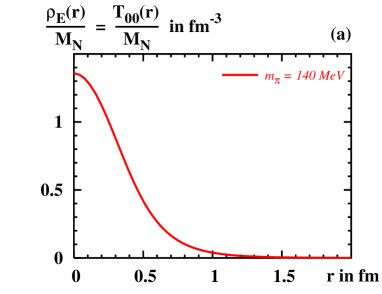
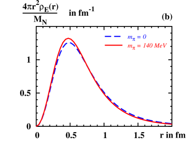
Figure 1: (a) The normalized energy density $\rho_{E}(r)/M_{N}$ of the nucleon as function of $r$ for the physical situation with $m_{\pi}=140\,{\rm MeV}$. The curve is normalized such that it yields unity upon integration over the entire volume. (b) The normalized energy density $4\pi r^{2}\rho_{E}(r)/M_{N}$ as function of $r$ in the chiral limit and for $m_{\pi}=140\,{\rm MeV}$. The curves are normalized such that one obtains unity upon integration over $r$.

Fig. 1a shows the normalized density $\rho_{E}(r)/M_{N}$ as function of $r$ for the physical situation with a pion mass of $140\,{\rm MeV}$. In this case in the model the nucleon mass is about $1250\,{\rm MeV}$. This overestimate of the physical nucleon mass of ${\cal O}(300\,{\rm MeV})$ is typical for the soliton approach and its origin is well-understood Pobylitsa:1992bk . In the center of the nucleon one finds $\rho_{E}(0)=1.7\,{\rm GeV\,fm}^{-3}$ or $3.0\times 10^{15}\,{\rm g\,\,cm}^{-3}$. In order to gain some intuition about this number we remark that this corresponds roughly to 13 times the equilibrium density of nuclear matter.

It is instructive to consider the energy density in the chiral limit. The result is shown in Fig. 1b where we compare $4\pi r^{2}\rho_{E}(r)/M_{N}$ as functions of $r$ for $m_{\pi}=0$ and $140\,{\rm MeV}$. The curves are normalized such that one obtains unity when integrating over $r$. Fig. 1b shows that with decreasing $m_{\pi}$ the energy density is spread more widely. This can be quantified by considering the $m_{\pi}$-dependence of the mean square radius of the energy density (23) defined as

$$\langle r_{E}^{2}\rangle=\frac{\int\!{\rm d}^{3}{\bf r}\;r^{2}\rho_{E}(r)}{\int\!{\rm d}^{3}{\bf r}\;\rho_{E}(r)}\;,$$ (51)

and which increases in the chiral limit, see Table 1. This is an intuitively expected feature. As the pion mass decreases, the range of the “pion cloud” increases and the nucleon becomes “larger”.

The popular idea of the nucleon consisting of a “quark core” surrounded by a “pion cloud” is strictly speaking well defined in models only. Here, in the CQSM, we shall associate the contribution of the discrete level as “quark core” and the contribution of the negative continuum states as “pion cloud”. From the long-distance behaviour of the soliton profile (29) one finds in the chiral limit

$$\rho_{E}(r)=\frac{f_{\pi}^{2}}{4}\;{\rm tr}_{F}\,\biggl{[}\nabla^{k}U({\bf r})\,\nabla^{k}U^{\dagger}({\bf r})\biggr{]}+\dots\;\stackrel{{\scriptstyle r\to\rm large}}{{\longrightarrow}}\;3\left(\frac{3g_{A}}{8\pi f_{\pi}}\right)^{2}\frac{1}{r^{6}}$$ (52)

where ${\rm tr}_{F}$ is the trace over flavour indices of the SU(2) matrices and the dots in the intermediate step denote terms which contain higher $U$-field derivative terms and vanish faster at large $r$ than the displayed leading term. The result (52) can be read off from Eq. (7.8) of Diakonov:1996sr . At $m_{\pi}\neq 0$ the decay of $\rho_{E}(r)$ at large $r$ is exponential due to the corresponding behaviour of the soliton profile (29). This diminishes the “range of the pion cloud” and reduces $\langle r_{E}^{2}\rangle$.

These observations can be further quantified by considering the chiral expansion of (51) which gives, see App. I,

$$\langle r_{E}^{2}\rangle=\langle\;\stackrel{{\scriptstyle\circ}}{{r}}{\!}_{E}^{2}\rangle-\frac{81\,g_{A}^{2}}{64\pi f_{\pi}^{2}M_{N}}\;m_{\pi}+\dots$$ (53)

Here and in the following the ^∘ above a quantity denotes its value in the chiral limit, and the dots denote terms vanishing faster in the chiral limit than the respective leading term. Considering the non-commutativity of the limits $N_{c}\to\infty$ and $m_{\pi}\to 0$ (see the discussion below in Sec. VIII) Eq. (53) agrees with chiral perturbation theory Belitsky:2002jp .

The term linear in $m_{\pi}$ in Eq. (53), i.e.  the leading non-analytic (in the current quark mass $m\propto m_{\pi}^{2}$) contribution to the mean square radius of the energy density accounts almost entirely for the reduction of $\langle r_{E}^{2}\rangle$ from $m_{\pi}=0$ to $140\,{\rm MeV}$, see Table 1. At the physical pion mass we find $\langle r_{E}^{2}\rangle=0.67\,{\rm fm}^{2}$. This value is similar to the electric charge radius of the proton. In fact, we observe a qualitative similarity of the energy density and electric proton charge distributions in the model Christov:1995hr ; Christov:1995vm .

VI Angular momentum density

Taking in Eq. (48) the limit $t\to 0$ yields

$$J(0)=\int\!{\rm d}^{3}{\bf r}\;\rho_{J}(r)\;,$$ (54)

which shows in which sense it is adequate to refer to $\rho_{J}(r)$ as the “angular momentum density”. In order to see that $J(0)=\frac{1}{2}$, i.e. that the constraint (13) is satisfied in the CQSM we insert (45) in the above equation and obtain

$$2J(0)=\frac{N_{c}}{12I}\!\sum_{{{\scriptscriptstyle{n,\rm occ}}\atop{\scriptscriptstyle{j,\rm non}}}}\epsilon^{abc}\langle j|\biggl{(}2\hat{p}^{a}\hat{r}^{b}+(E_{n}+E_{j})\gamma^{0}\gamma^{a}\hat{r}^{b}\biggr{)}|n\rangle\;\frac{\langle n|\tau^{c}|j\rangle}{E_{j}-E_{n}}\,\biggl{|}_{\rm reg}\stackrel{{\scriptstyle\mbox{\footnotesize Ref.~{}\cite[cite]{\@@bibref{Authors Phrase1YearPhrase2}{Ossmann:2004bp}{\@@citephrase{(}}{\@@citephrase{)}}}}}}{{=}}\int\limits_{-1}^{1}\!dx\;x\,\sum\limits_{f}(H^{f}+E^{f})(x,\xi,0)\stackrel{{\scriptstyle\mbox{\footnotesize Ref.~{}\cite[cite]{\@@bibref{Authors Phrase1YearPhrase2}{Ossmann:2004bp}{\@@citephrase{(}}{\@@citephrase{)}}}}}}{{\equiv}}1\,.$$ (55)

In the intermediate step in Eq. (55) we recovered the model expression for the second moment of $\sum_{f}(H^{f}+E^{f})(x,\xi,t)$ at $t=0$, see Appendix C of Ossmann:2004bp . This sum rule, which follows from adding up Eqs. (3) and (4), was explicitly proven to be satisfied in the model in Ossmann:2004bp . In the model the entire nucleon spin is due to the spin and orbital angular momentum of quarks and antiquarks, and hence $2J(0)=1$ Ossmann:2004bp . This again is a correct and consistent result since there are no explicit gluon degrees of freedom in the CQSM.

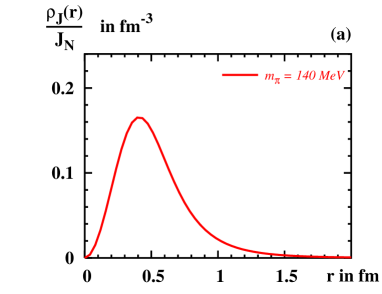
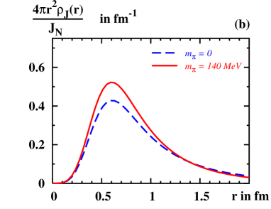
Figure 2: (a) The normalized angular momentum density $\rho_{J}(r)/J_{N}$ as function of $r$ for the physical situation with $m_{\pi}=140\,{\rm MeV}$. The curve is normalized such that it yields unity upon integration over the entire volume. (b) The normalized angular momentum density $4\pi r^{2}\rho_{J}(r)/J_{N}$ as function of $r$ for $m_{\pi}=0$ and $140\,{\rm MeV}$. The curves are normalized such that one obtains unity upon integration over $r$.

The numerical result for the normalized angular momentum density $\rho_{J}(r)/J_{N}\equiv 2\rho_{J}(r)$ as function of $r$ for the physical situation is shown in Fig. 2a. ($J_{N}=\frac{1}{2}$ denotes the nucleon spin.) We observe that $\rho_{J}(r)\propto r^{2}$ at small $r$.

In Fig. 2b we compare the normalized angular momentum densities $4\pi r^{2}\rho_{J}(r)/J_{N}$ as functions of $r$ for $m_{\pi}=0$ and $140\,{\rm MeV}$. These curves are normalized such that one obtains unity upon integration over $r$. Within the rotating soliton picture the result is reasonable. The smaller $m_{\pi}$, the larger the nucleon, and the more important is the role of the region of large $r$ for the description of the soliton rotation, i.e. for the spin structure of the nucleon. This is reflected by the mean square radius of the angular momentum density which we define in analogy to (51) as

$$\langle r_{J}^{2}\rangle=\frac{\int\!{\rm d}^{3}{\bf r}\;r^{2}\rho_{J}(r)}{\int\!{\rm d}^{3}{\bf r}\;\rho_{J}(r)}\;.$$ (56)

The mean square radius of the angular momentum density increases with decreasing $m_{\pi}$, see Table 1. In the chiral limit $\rho_{J}(r)\propto\frac{1}{r^{4}}$ at large $r$, i.e. $\langle r_{J}^{2}\rangle$ diverges in the chiral limit. As a consequence $J(t)$ has an infinitely steep slope at $t=0$ in the chiral limit, see Sec. VIII and Appendix I for further discussions.

VII Pressure, shear forces, soliton stability, and sign of $d_{1}$

For the pressure (44) the analogon of the “normalization relations”, Eqs. (49) and (55), of the other densities is the stability criterion (16). Integrating the $r^{2}$-weighted model expression for $p(r)$ over $r$ we obtain

$$\int\limits_{0}^{\infty}\!\!{\rm d}r\,r^{2}p(r)\equiv\frac{N_{c}}{12\pi}\int\!{\rm d}^{3}{\bf x}\sum_{n,\,\rm occ}\phi_{n}^{\ast}({\bf x})\,(\gamma^{0}{{{\mbox{\boldmath$\gamma$}}}}\hat{\bf p})\,\phi_{n}({\bf x})=\frac{N_{c}}{12\pi}\sum_{n,\,\rm occ}\langle n|\,\gamma^{0}{{\mbox{\boldmath$\gamma$}}}\hat{\bf p}\,|n\rangle=0\,,$$ (57)

because more generally the tensor $K^{ij}$ defined as

$$K^{ij}=\sum_{n,\,\rm occ}\langle n|\,\gamma^{0}\gamma^{i}\hat{p}^{j}\,|n\rangle\stackrel{{\scriptstyle\mbox{\footnotesize{Ref.~{}\cite[cite]{\@@bibref{Authors Phrase1YearPhrase2}{Diakonov:1996sr}{\@@citephrase{(}}{\@@citephrase{)}}}}}}}{{=}}0\;$$ (58)

is zero — however, if and only if, one evaluates the expression (58) with the self-consistent profile, i.e.  with that profile which minimizes the soliton energy (27). This was proven in Ref. Diakonov:1996sr . Thus, the stability criterion (16) is satisfied.

Next let us check that one obtains in the model the correct result for the constant $d_{1}=d_{1}(0)$ defined in Eq. (13). Expanding the expression (47) around small $t$ we obtain

$$d_{1}(t)=\frac{15M_{N}}{2}\int\!{\rm d}^{3}{\bf r}\;p(r)\;\biggl{(}\frac{1}{t}+\frac{r^{2}}{3!}+{\cal O}(t)\biggr{)}\;.$$ (59)

Due to (57) the $1/t$-term drops out, and we verify in the CQSM the relation (II) between $d_{1}$ and the pressure.

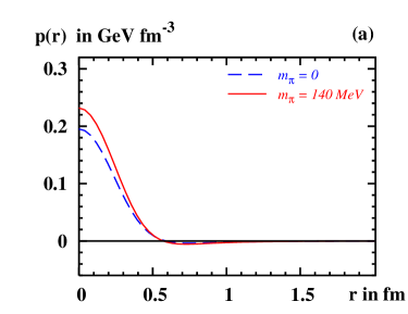
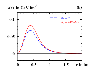
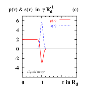
Figure 3: (a) The pressure $p(r)$ as function of $r$ for $m_{\pi}=0$ and $140\,{\rm MeV}$. (b) The same for the function $s(r)$ defined in Eq. (14) which describes the shear forces in the nucleon, and is related to $p(r)$ by the relation (15). (c) $p(r)$ and $s(r)$ in a liquid drop in units of $\gamma/R_{d}$ as functions of $r$ in units of $R_{d}$. Here $R_{d}$ is the radius of the drop, and $\gamma$ is the surface tension. The $\delta$-functions in $p(r)$ and $s(r)$ in Eq. (60) are smeared for better visibility, see text.

Fig. 3a shows the pressure $p(r)$ as function of $r$. In the physical situation $p(r)$ takes its global maximum at $r=0$ with $p(0)=0.23\,{\rm GeV}/{\rm fm}^{3}=3.7\cdot 10^{34}\,{\rm Pa}$. This is ${\cal O}(10\!-\!100)$ higher than the pressure inside a neutron star Prakash:2000jr . Then $p(r)$ decreases monotonically — becoming zero at $r_{0}=0.57\,{\rm fm}$ — till reaching its global minimum at $r_{p,\,\rm min}=0.72\,{\rm fm}$, after which it increases monotonically remaining, however, always negative. The positive sign of the pressure for $r<r_{0}$ corresponds to repulsion, while the negative sign in the region $r>r_{0}$ means attraction.

In Fig. 3a we see how the pressure depends on the pion mass. The pressure in the center of the nucleon increases as $m_{\pi}$ increases — obvious consequence of the fact that the (energy) density also increases, see Table 1. As a response to the increased $p(r)$ at small $r$ — keep in mind the stability condition (16) — the pressure takes also larger absolute values in the region $r>r_{0}$ where it is negative. This can again be intuitively understood because a heavier particle is more tightly bound, i.e. the attractive forces are stronger. The zero of $p(r)$ moves towards smaller values of $r$ with increasing $m_{\pi}$, see Table 1.

In Fig. 3b we show the distribution of the shear forces $s(r)$ obtained from our results for $p(r)$ by solving the differential equation (15). The distribution of shear forces is always positive. It reaches for $m_{\pi}=140\,{\rm MeV}$ a global maximum at $r=0.40\,{\rm fm}$. The position of the maximum is weakly dependent on $m_{\pi}$. At small $r$ we observe $s(r)\propto r^{2}$.

It is interesting to compare to which extent the nucleon “resembles” a liquid drop of radius $R_{d}$ with constant density and constant pressure $p_{0}$ inside. In such a drop the pressure and shear forces are given by Polyakov:2002yz

$$p(r)=p_{0}\,\theta(R_{d}-r)-\frac{1}{3}\;p_{0}R_{d}\,\delta(R_{d}-r)\;\;\;\;\mbox{and}\;\;\;\;s(r)=\gamma\,\delta(R_{d}-r)\;,$$ (60)

where $\gamma=\frac{1}{2}\;p_{0}R_{d}$ denotes the surface tension. We show this situation in Fig. 3c — where, however, for better visibility the $\delta$-functions in (60) are smeared out. This corresponds to allowing the density in the drop to decrease continuously from its constant inner value to zero over a finite “skin” (of the size $\sim\frac{1}{10}R_{d}$ in Fig. 3c).

Comparing the liquid drop picture to the results from the CQSM we observe a remote qualitative similarity. In contrast to the liquid drop, the density “inside” the nucleon is far from being constant, see Fig. 1a, and one cannot expect the pressure in the nucleon to exhibit a constant plateau as in the liquid drop. Still the pressure exhibits the same qualitative features. The shear forces become maximal in the vicinity of what can be considered as the “edge” of the object. This is the case in particular for the liquid drop However, the “edge” of nucleon is far more diffuse, and the distribution of shear forces $s(r)$ is widespread. Of course, the nucleon can hardly be considered a liquid drop. Such an analogy might be more appropriate for nuclei Polyakov:2002yz . Nevertheless this comparison gives some intuition on the model results — in particular, about the qualitative shape of the distributions of pressure and shear forces.

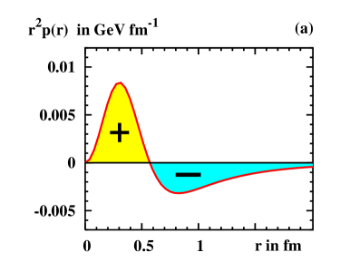
Figure 4: (a) $r^{2}p(r)$ as function of $r$ from the CQSM at the physical value of $m_{\pi}$. The shaded regions have — within the numerical accuracy of about half percent — the same surface areas. This shows how the stability condition $\int_{0}^{\infty}\!{\rm d}r\,r^{2}p(r)=0$ in Eq. (57) is realized.
(b) The same as (a) but with an additional power of $r^{2}$ and the prefactor $5\pi M_{N}$. Integrating this curve over $r$ yields $d_{1}$ according to (II). The plot shows that one obtains a negative sign for $d_{1}$ as a consequence of the stability condition (16) shown in Fig. 4a.

Next let us discuss how the stability condition (57) is satisfied. Fig. 4a shows $r^{2}p(r)$ as function of $r$. The shaded regions have the same surface areas but opposite sign and cancel each other — within numerical accuracy

$$\int\limits_{0}^{r_{0}}\!{\rm d}r\;r^{2}p(r)=2.61\,{\rm MeV}\,,\;\;\;\;\int\limits_{r_{0}}^{\infty}\!{\rm d}r\;r^{2}p(r)=-2.63\,{\rm MeV}\,.$$ (61)

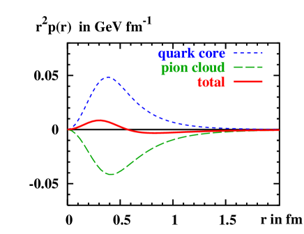
Figure 5: The pressure $p(r)$ as function of $r$ for $m_{\pi}=140\,{\rm MeV}$. Dotted line: Contribution of the discrete level associated with the quark core. Dashed line: Continuum contribution associated with the pion cloud. Solid line: The total result.

In order to better understand how the soliton acquires stability, it is instructive to look in detail how the total pressure is decomposed of the separate contributions of the discrete level and the continuum contribution. Fig. 5 shows that the contribution of the discrete level is always positive. This contribution corresponds in model language to the contribution of the “quark core” and one expects a positive contribution (“repulsion”) due to the Pauli principle. At large $r$ the discrete level contribution vanishes exponentially since the discrete level wave-function does so Diakonov:1987ty .

The continuum contribution is throughout negative — as can be seen from Fig. 5 and can be understood as follows. The continuum contribution can be interpreted as the effect of the pion cloud which in the model is responsible for the forces binding the quarks to form the nucleon. I.e.  it provides a negative contribution to the pressure corresponding to attraction. In the chiral limit the continuum contribution exhibits a power-like decay which dictates the long-distance behaviour of the total result for the pressure as follows

$$p(r)=-\left(\frac{3g_{A}}{8\pi f_{\pi}}\right)^{2}\frac{1}{r^{6}}\;\;\;\;\mbox{and}\;\;\;\;s(r)=3\left(\frac{3g_{A}}{8\pi f_{\pi}}\right)^{2}\frac{1}{r^{6}}\;\;\;\;\;\;\mbox{at large $r$.}$$ (62)

where for completeness we quote also the result for $s(r)$. For $m_{\pi}\neq 0$ the continuum contribution exhibits an exponential decay at large $r$ due to the Yukawa tail of the soliton profile (29) — like the contribution of the discrete level, however, it still dominates the behaviour of the total result. Fig. 5 reveals that the actual cancellation between the different contributions leading to (57) are even more impressive than we could guess considering the numbers in Eq. (61). For $m_{\pi}=140\,{\rm MeV}$ we obtain the following numbers, and see that the two contributions cancel each other within numerical accuracy

$$\int\limits_{0}^{\infty}\!{\rm d}r\;r^{2}p(r)\biggl{|}_{\rm lev}=26.69\,{\rm MeV}\,,\;\;\;\;\int\limits_{0}^{\infty}\!{\rm d}r\;r^{2}p(r)\biggl{|}_{\rm cont}=-26.71\,{\rm MeV}\,.$$ (63)

Finally, we discuss the relation of stability and the sign of the constant $d_{1}$. By comparing Figs. 4a and 4b we immediately understand that in the CQSM the constant $d_{1}$ takes a negative value

$$d_{1}<0\,.$$ (64)

This result is presumably of general character. In fact, the observation (64) follows naturally from our intuition on the pressure and shear forces distributions we gained from our study. It seems physically intuitive that in a mechanically stable object the following conditions hold

(I) $$\mbox{for a stable object the pressure has the shape}\;\;\;\;\displaystyle p(r)\;\cases{>0&for $r<r_{0}$\cr=0&for $r=r_{0}$\cr<0&for $r>r_{0}$}$$

(II) $$\mbox{distribution of shear forces satisfies for all $r$}\;\;\;\;\;\;s(r)>0\;.$$

From (I) and the stability criterion (16) we conclude that $d_{1}\propto\int_{0}^{\infty}\!{\rm d}r\,r^{4}p(r)<0$ as illustrated in Figs. 4a and 4b. The same conclusion follows from (II) using $d_{1}\propto-\int_{0}^{\infty}\!{\rm d}r\,r^{4}s(r)<0$ in (II).

Of course, one can imagine a pressure distribution with more zeros and a different shape than in (I) still yielding (64). However, (I) is the simplest case which one may expect to hold for a ground state — like the nucleon. Such a ground state object is characterized by having one “surface” only, although a quite smeared out one in the case of the nucleon, hence the condition (II). A more complicated distribution of the pressure — with more zeros, i.e. also more maxima and minima — would imply an object with several (smeared out) surfaces, which follows from the last condition in App. B.

The conjecture (64) is — besides being physically appealing— in agreement with all available information on $d_{1}$, see Sec. II. One may therefore suspect that (64) is a general theorem which connects the stability of an object to the sign of its constant $d_{1}$. However, such a theorem — if it exists — remains to be rigorously proven for the general case.

VIII Results for the form factors

From the densities $\rho_{E}(r)$, $\rho_{J}(r)$ and $p(r)$ which we discussed in detail in Secs. V, VI and VII we obtain the form factors of the EMT by means of Eqs. (46, 47, 48). The results are shown in Fig. 7 for $m_{\pi}=0$ and $140\,{\rm MeV}$. In the CQSM the form factors $M_{2}(t)$, $J(t)$ are normalized at $t=0$ as $M_{2}(0)=2J(0)=1$ as proven in Secs. V and VI. The numerical results satisfy these constraints within a numerical accuracy of (1-2)$\%$, see Figs. 7a and 7b.

In contrast, the normalization of the form factor $d_{1}(t)$ at $t=0$ is not known a priori. We find $d_{1}=d_{1}(0)<0$ as anticipated in Sec. VII. The constant $d_{1}$ has a well-defined chiral limit. This can be concluded from Eq. (II) which relates $d_{1}$ to the distributions of pressure or shear forces, and from the fact that $p(r)$ and $s(r)$ drop off sufficiently fast at large $r$ in the chiral limit, see (62).

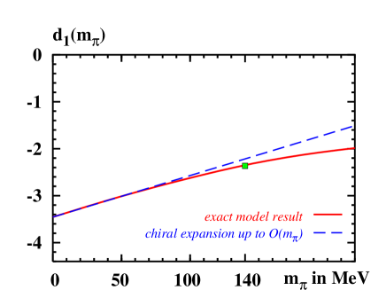
Figure 6: The constant $d_{1}$ as function of $m_{\pi}$. Comparison of the full CQSM result, and the expansion of $d_{1}(m_{\pi})$ up the leading non-analytic term according to Eq. (65). The square marks the physical point.

The absolute value of $d_{1}$ decreases with increasing $m_{\pi}$ and we observe a strong sensitivity of $d_{1}$ to $m_{\pi}$. That this is not surprizing can be understood by considering the chiral expansion of $d_{1}$. Expanding $d_{1}(m_{\pi})$ in the model for small $m_{\pi}$ we obtain, cf. Appendix I,

$$d_{1}(m_{\pi})=\;\;\stackrel{{\scriptstyle\circ}}{{d_{1}}}\;+\;\frac{15\,g_{A}^{2}M_{N}}{64\,\pi\,f_{\pi}^{2}}\;m_{\pi}+\dots$$ (65)

Thus, we see that $d_{1}(m_{\pi})$ receives a large leading non-analytic contribution in the current quark mass $m\propto m_{\pi}^{2}$, which is the origin of the strong $m_{\pi}$-dependence of $d_{1}(m_{\pi})$. The expansion (65) approximates in the model $d_{1}(m_{\pi})$ to within an accuracy of $15\%$ up to the physical point. At the physical point the absolute value of $d_{1}$ is reduced by about $30\,\%$ with respect to its chiral limit value. The numerical results for $d_{1}$ are summarized in Table 1.

Next, let us focus on the derivatives of the form factors at $t=0$. From Eq. (11) we conclude that at $t=0$ the slope of the form factor $M_{2}(t)$ is given by

$$M_{2}^{\prime}(0)=\frac{\langle r_{E}^{2}\rangle}{6}+\frac{d_{1}}{5M_{N}^{2}}=\;\stackrel{{\scriptstyle\circ}}{{M}}{\!}_{2}^{\prime}(0)-\frac{21\,g_{A}^{2}}{128\pi f_{\pi}^{2}}\;\frac{m_{\pi}}{M_{N}}+\dots$$ (66)

where the chiral expansion follows from (53) and (65). In particular, $M_{2}^{\prime}(0)$ is well-defined for all $m_{\pi}$ including the chiral limit. The situation is different for the form factors $J(t)$ and $d_{1}(t)$. The slope of $J(t)$ at $t=0$ can be deduced from (48) and is given by

$$J^{\prime}(0)=\frac{\langle r_{J}^{2}\rangle}{6}$$ (67)

with $\langle r_{J}^{2}\rangle$ defined in (56). Since the mean square radius of the angular momentum density diverges in the chiral limit, see Sec. VI, so does $J^{\prime}(0)$. See also the discussion in App. I.

That also the slope of $d_{1}(t)$ becomes infinitely steep at $t=0$ can be understood as follows. From Eqs. (11, 14, 15) it follows that the derivative of $d_{1}(t)$ at $t=0$ be expressed as

$$d_{1}^{\,\prime}(t)\biggl{|}_{t=0}=-\frac{M_{N}}{42}\,\int\!{\rm d}^{3}{\bf r}\;r^{4}s(r)=\frac{M_{N}}{16}\,\int\!{\rm d}^{3}{\bf r}\;r^{4}p(r)\;.$$ (68)

Since in the chiral limit $p(r)$ and $s(r)$ drop off as $\frac{1}{r^{6}}$ at large $r$ we see that $\;\stackrel{{\scriptstyle\circ}}{{d_{1}^{\,\prime}}}\!(0)$ diverges as $m_{\pi}\to 0$.

To make this statement more quantitative let us expand $d_{1}(t)$ in the chiral limit in the model for small $t$. We obtain

$$\;\stackrel{{\scriptstyle\circ}}{{d_{1}}}\!(t)=\;\stackrel{{\scriptstyle\circ}}{{d_{1}}}-\frac{45\,g_{A}^{2}M_{N}}{512\,f_{\pi}^{2}}\;\sqrt{-t}+{\cal O}(t)\;,$$ (69)

which means that in the chiral limit $\;\stackrel{{\scriptstyle\circ}}{{d_{1}^{\,\prime}}}\!(t)\propto 1/\sqrt{-t}$ at small $t$. Alternatively, one may keep $m_{\pi}\neq 0$, evaluate the derivative of $d_{1}(t)$ at $t=0$, and then consider small $m_{\pi}$. (Note that the limits $m_{\pi}\to 0$ and $t\to 0$ do not commute.) Then we find that the slope of $d_{1}(t)$ at $t=0$ diverges in the chiral limit as

$$\;\stackrel{{\scriptstyle\circ}}{{d_{1}^{\,\prime}}}\!(t)\biggl{|}_{t=0}=-\frac{3\,g_{A}^{2}\,M_{N}}{32\,\pi f_{\pi}^{2}\,m_{\pi}}+\dots\;.$$ (70)

The results (70) and (70) are derived in Appendix I. The numerical results for $J(t)$ and $d_{1}(t)$ in Figs. 7b and 7c indicate the infinitely steep slopes at $t=0$ within the numerical accuracy.

Notice that we derived the analytical results in (68, 69, 70) in the framework of the CQSM. However, the leading non-analytic terms (i.e. terms $\propto m_{\pi}$) in the chiral expansion of $d_{1}(t)$ in (68, 69, 70) are dictated by chiral symmetry breaking, and are independent of the details of the chiral theory chosen to derive them. In fact, our results (68, 69, 70) agree with those obtained from chiral perturbation theory in Ref. Belitsky:2002jp — provided one takes into account an important difference. The CQSM is formulated in the large-$N_{c}$ limit which does not commute with the chiral limit Dashen:1993jt . At large $N_{c}$ the masses of the nucleon and $\Delta$-resonance are degenerated: $M_{\Delta}-M_{N}={\cal O}(N_{c}^{-1})$. Therefore in the CQSM — in addition to the nucleon considered in chiral perturbation theory Belitsky:2002jp — the $\Delta$-resonance contributes on equal footing as intermediate state in chiral loops. Considering that in the large $N_{c}$-limit the pion-Delta-nucleon and pion-nucleon-nucleon couplings are related as $g_{\pi N\Delta}=\frac{3}{2}g_{\pi NN}$ (phenomenologically satisfied to a very good approximation), one finds that the $\Delta$-resonance makes a contribution to leading non-analytic terms which is — for scalar-isoscalar quantities —two times larger than that of the nucleon Cohen:1992uy . Hence, our leading non-analytic terms in Eqs. (68, 69, 70) are 3 times larger than those obtained from chiral perturbation theory in Ref. Belitsky:2002jp where $N_{c}$ was kept finite. Other examples of the derivation of leading non-analytic terms in chiral soliton models can be found in Schweitzer:2003sb ; Cohen:1992uy .

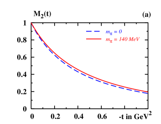
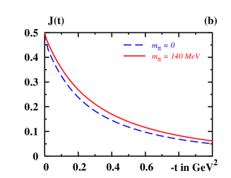
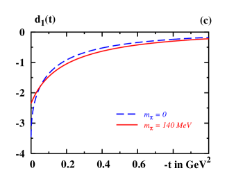
Figure 7: The form factors of the energy momentum tensor $M_{2}(t)$, $J(t)$ and $d_{1}(t)$ as functions of $t$ for the pion masses $m_{\pi}=0$, $140\,{\rm MeV}$. All form factors can be well approximated by dipole fits, however, with the exception of $J(t)$ and $d_{1}(t)$ in the chiral limit which exhibit infinitely steep slopes at $t=0$, see text.

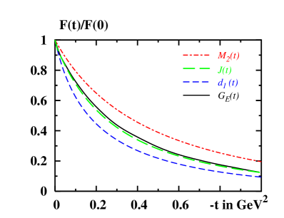
Figure 8: EMT form factors as functions of $t$. Dashed-dotted line: $M_{2}(t)$. Long-dashed line: $J(t)$. Dashed line: $d_{1}(t)$; all computed here. Solid line: electric proton form factor $G_{E}(t)$ from Ref. Christov:1995hr . All form factors refer to the physical pion mass, and are normalized with respect to their values at $t=0$.

Next, we turn to the discussion of the $t$-dependence of the form factors, and recall that in the large-$N_{c}$ limit we strictly speaking are restricted to $|t|\ll M_{N}^{2}$. However, in practice it is observed that the CQSM provides reliable results for electromagnetic form factors up to $|t|\lesssim 1\,{\rm GeV}^{2}$ Christov:1995hr ; Christov:1995vm .

Fig. 7 shows the form factors of the EMT as functions of $t$ for $|t|\leq 1\,{\rm GeV}^{2}$ for $m_{\pi}=0$ and $140\,{\rm MeV}$. For $m_{\pi}\neq 0$ the form factors can be well approximated by dipole fits

$$F(t)=\frac{F(0)}{(1-t/M_{\rm dip}^{2})^{2}}$$ (71)

with the values for the dipole masses quoted in Table 1.

It is instructive to compare these results within the model to the electromagnetic form factors — for definiteness we choose the electric form factor of the proton $G_{E}(t)$ computed in the CQSM in Ref. Christov:1995hr . Fig. 8 shows that $J(t)$ and $G_{E}(t)$ exhibit a similar $t$-dependence. However, $M_{2}(t)$ falls off with increasing $|t|$ slower than $G_{E}(t)$, while $d_{1}(t)$ shows a faster fall off.

One popular assumption in literature in the context of modelling GPDs is to assume a generic factorized Ansatz of the type $H(x,\xi,t)=H(x,\xi)G(t)$ where $G(t)$ denotes the respective form factor (other approaches are discussed in Goeke:2001tz ; Belitsky:2001ns ; Diehl:2004cx ; Guidal:2004nd ; Radyushkin:2004mt ; Vanderhaeghen:2004sa ). This assumption implies that the form factors of the EMT should have approximately the same $t$-dependence as the electromagnetic form factors. Our results indicate that this is quite a rough approximation, and support the observations that in the CQSM $H(x,\xi,t)\neq H(x,\xi)G(t)$, see Refs. Goeke:2001tz ; Petrov:1998kf

Let us compare our result for $d_{1}$ with the result from direct calculations of GPDs in the model Petrov:1998kf which yield $d_{1}^{Q}\approx-8.0$ at the low model scale in the chiral limit. The discrepancy with the corresponding results in Table 1 is due to the fact that in Petrov:1998kf the momentum-dependent constituent mass $M(p)$ was employed vs. our proper-time or Pauli-Villars regularization with $M={\rm const}$, and that the approximative “interpolation formula” was used vs. the exact numerical calculation done here.

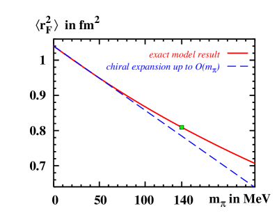
Figure 9: Mean square radius of EMT trace operator vs. $m_{\pi}$.

For the mean square radius $\langle r_{F}^{2}\rangle$ of the operator of the EMT trace, see Eqs. (23, 24), we obtain in the chiral limit

$$\langle\;\stackrel{{\scriptstyle\circ}}{{r}}{\!}_{F}^{2}\rangle=(1.0-1.2)\,{\rm fm}^{2}$$ (72)

while its value at the physical point is reduced by about $0.2\,{\rm fm}$ compared to (72), see Table 1. From the chiral expansion of $\langle r_{F}^{2}\rangle$ which follows from Eqs. (53, 65, 24) and reads

$$\langle r_{F}^{2}\rangle=\langle\;\stackrel{{\scriptstyle\circ}}{{r}}{\!}_{F}^{2}\rangle-\frac{117\,g_{A}^{2}}{64\pi f_{\pi}^{2}M_{N}}\;m_{\pi}+\dots\;,$$ (73)

we see that the leading non-analytic term in (73) explains the main portion of the observed reduction of $\langle r_{F}^{2}\rangle$ at the physical point compared to its chiral limit value, see Fig. 9.

It is instructive to compare our result (72) for the mean square radius of the EMT trace to the mean square radius of the traceless part of the EMT $(0.3\,{\rm fm})^{2}$ estimated by means of QCD sum rules Braun:1992jp . The instanton vacuum model provides a possible explanation why the radius of the trace of the EMT is so much larger than the traceless part. In chiral limit the trace part is basically the gluonic operator $F_{\mu\nu}F^{\mu\nu}$ which is due to one-instanton contributions and appears in leading order in the instanton packing fraction. The traceless part arises from instanton-anti-instanton contributions which appear at subleading order Diakonov:1995qy .

Table 1: The pion mass dependence of different quantities computed in the CQSM: the energy density in the center of the nucleon $\rho_{E}(0)$, the mean square radii $\langle r_{E}^{2}\rangle$ and $\langle r_{J}^{2}\rangle$ as defined in Eqs. (51, 56), the pressure $p(0)$ in the center of the nucleon, the zero of the pressure defined as $p(r_{0})=0$, the constant $d_{1}$, the dipole masses of the form factors $M_{2}(t)$, $J(t)$ and $d_{1}(t)$ as defined in Eq. (71), and the mean squared radius of the trace of the EMT (22). In the chiral limit $J(t)$ and $d_{1}(t)$ have infinitely steep slopes at $t=0$. In these cases dipole fits do not provide useful approximations and are undefined (labelled by “—” in the Table). The proper time regularization can be applied, in principle, to any $m_{\pi}$ Goeke:2005fs . The Pauli-Villars regularization is applicable only for $m_{\pi}=0$ Kubota:1999hx .

	$m_{\pi}$	$\rho_{E}(0)$	$\langle r_{E}^{2}\rangle$	$\langle r_{J}^{2}\rangle$	$p(0)$	$r_{0}$	$d_{1}$	dipole masses $M_{\rm dip}$ in GeV for			$\langle r_{F}^{2}\rangle$
	${\rm MeV}$	${\rm GeV}/{\rm fm}^{3}$	${\rm fm}^{2}$	${\rm fm}^{2}$	${\rm GeV}/{\rm fm}^{3}$	${\rm fm}$		$M_{2}(t)$	$J(t)$	$d_{1}(t)$	${\rm fm}^{2}$
proper time regularization:
	0	1.54	0.79	$\infty$	0.195	0.59	-3.46	0.867	—	—	1.01
	50	1.57	0.76	1.42	0.202	0.59	-3.01	0.873	0.692	0.519	0.95
	140	1.70	0.67	1.32	0.232	0.57	-2.35	0.906	0.745	0.646	0.81
Pauli-Villars regularization:
	0	0.75	0.86	$\infty$	0.332	0.63	-4.75	0.804	—	—	1.24

IX Conclusions

In this work we presented a study of the form factors of the EMT in the large-$N_{c}$ limit in the framework of the CQSM. We provided numerous checks of the theoretical consistency of the model results. Among others, we demonstrated that the same model expressions for the form factors can be derived from the EMT and from GPDs.

We computed the spatial density distributions, and mean square radii of the operators of different components of the EMT and its trace. Interesting results are that the energy density related to $\hat{T}^{00}$ in the center of the nucleon is about $1.7\,{\rm GeV}^{-3}$, i.e. about 13 times higher then the equilibrium density of nuclear matter. The mean square radius of the operator $\hat{T}^{00}$ is about $0.67\,{\rm fm}^{2}$. For the mean square radius of the “angular momentum distribution” related to the operator $\hat{T}^{0k}$ ($k=1,\,2,\,3$) we find a much larger value $1.32\,{\rm fm}^{2}$.

We studied the spatial distribution of strong forces in the nucleon as described in terms of the distributions of pressure and shear forces which are defined by the spatial components $\hat{T}^{jk}$ ($j,\,k=1,\,2,\,3$) of the EMT. As a byproduct of this study we learned how the soliton acquires stability in the CQSM — namely due to subtle balance of repulsive forces in the center due the “quark core” and attractive forces in the outskirts of the nucleon due the “pion cloud” which bounds the quarks in the model.

We observed a physically appealing connection between the criterion for the stability of a particle, and the sign of the constant $d_{1}$, i.e. the form factor $d_{1}(t)$ at zero-momentum transfer. Our observations imply that for a stable particle one always has $d_{1}<0$, though we cannot prove this conjecture for the general case. All available results for $d_{1}$ in literature are compatible with this observation.

We derived the leading non-analytic chiral contributions to the form factors in the large $N_{c}$ limit, which agree with results from chiral perturbation theory Chen:2001pv ; Belitsky:2002jp ; Diehl:2006ya provided one takes into account that the limits $N_{c}\to\infty$ and $m_{\pi}\to 0$ do not commute Dashen:1993jt ; Cohen:1992uy .

We observed that the model results for the form factors of the EMT can, for $m_{\pi}>0$, be well approximated by dipole fits. The different form factors have different $t$-dependences. For $J^{Q}(t)$ we obtain in the model a dipole mass similar to that of the electromagnetic form factors of the proton. The dipole mass of $M_{2}(t)$ is much larger than that, while that of $d_{1}(t)$ is substantially smaller. These results are of interest for the phenomenology of hard exclusive reactions, and in particular for the task of extrapolating $J^{Q}(t)$ to $t=0$ which is necessary to extract from data information on what portion of the nucleon spin is due to quarks.

Our results yield in the chiral limit for the constant $d_{1}=-(3.5-4.8)$ depending on the regularization and confirm sign and — within model accuracy — magnitude of previous results Petrov:1998kf ; Kivel:2000fg . We observe, however, also a strong $m_{\pi}$-dependence of $d_{1}$ which is dominated by a sizeable leading non-analytic (in the current quark mass) contribution proportional to $m_{\pi}$. The latter is responsible for reducing the absolute value of $d_{1}$ by about $30\%$ at the physical point compared to its chiral limit value.

We estimated the mean square radius of the EMT trace operator to be about $(1\,{\rm fm})^{2}$ which appears much larger than the corresponding mean square radius of the traceless part of the EMT found to be $(0.3\,{\rm fm})^{2}$ Braun:1992jp , and noticed that the instanton vacuum model provides a possible explanation for that.

A study of the $m_{\pi}$-dependence of the EMT form factors in the model at larger values of $m_{\pi}$ in the spirit of Ref. Goeke:2005fs and a detailed comparison of the model results to lattice QCD data Mathur:1999uf ; Gadiyak:2001fe ; Hagler:2003jd ; Gockeler:2003jf ; Negele:2004iu ; Schroers:2007qf will be presented elsewhere accompanying-paper .

Acknowledgements    We thank Pavel Pobylitsa for fruitful discussions and valuable comments. This research is part of the EU integrated infrastructure initiative hadron physics project under contract number RII3-CT-2004-506078, and partially supported by the Graduierten-Kolleg Bochum-Dortmund and Verbundforschung of BMBF. A. S.  acknowledges support from GRICES and DAAD.

Note added    After this work was completed the work Wakamatsu:2007uc appeared where in particular the constant $d_{1}$ was studied. For $d_{1}^{u+d}$ similar results were obtained using somehow different model parameters. Interesting is the estimate for the flavour combination $d_{1}^{u-d}$ which was found rather small and confirms the large-$N_{c}$ prediction (18).

Appendix A Alternative definition of form factors

The following alternative definition of form factors of the EMT is commonly used in literature, see e.g. Ji:1996ek ,

$$\langle p^{\prime}|\hat{T}_{\mu\nu}^{Q,G}(0)|p\rangle = \bar{u}(p^{\prime})\biggl{[}A^{Q,G}(t)\,\frac{\gamma_{\mu}P_{\nu}+\gamma_{\nu}P_{\mu}}{2}+B^{Q,G}(t)\,\frac{i(P_{\mu}\sigma_{\nu\rho}+P_{\nu}\sigma_{\mu\rho})\Delta^{\rho}}{4M_{N}}$$ (74)

$$+ C^{Q,G}(t)\,\frac{\Delta_{\mu}\Delta_{\nu}-g_{\mu\nu}\Delta^{2}}{M_{N}}\pm\bar{c}(t)g_{\mu\nu}\biggr{]}u(p)\,.$$

By means of the Gordon identity $2M_{N}\bar{u}^{\prime}\gamma^{\alpha}u=\bar{u}^{\prime}(i\sigma^{\alpha\kappa}\Delta_{\kappa}+2P^{\alpha})u$ Eq.(74) can be rewritten as Eq.(1) with

$$A^{Q,G}(t) = M_{2}^{Q,G}(t)\phantom{\frac{1}{1}}$$

$$A^{Q,G}(t)+B^{Q,G}(t) = 2\,J^{Q,G}(t)$$

$$C^{Q,G}(t) = \frac{1}{5}\,d_{1}^{Q,G}(t)\,.$$ (75)

The constraints (13) translate in this language into $A^{Q}(0)+A^{G}(0)=1$ and $B^{Q}(0)+B^{G}(0)=0$. The latter constraint means that the total nucleon ”gravitomagnetic moment” vanishes.

In models, in which the only dynamical degrees of freedom are effective quark degrees of freedom, the constraint $B^{Q}(0)=0$ must hold. Such is the situation in the CQSM where consequently this constraint is satisfied Ossmann:2004bp .

Interestingly, it was argued Teryaev:1998iw that also in QCD the quark and gluon gravitomagnetic moments of the nucleon could vanish separately, i.e. $B^{Q}(0)=0$ and $B^{G}(0)=0$. That would imply that $M_{2}^{Q}(0)=2J^{Q}(0)$ and $M_{2}^{G}(0)=2J^{G}(0)$ at any scale, and not only in the asymptotic limit of a large renormalization scale Ji:1996ek , see Teryaev:1998iw for details.

Appendix B General relations from the conservation of EMT

Here we collect some worthwhile noticing relations for $p(r)$ and $s(r)$ which can be derived from the differential equation (15) — i.e.  which follow from the conservation of the EMT.

• For any $s(r)$ one obtains from (15) a $p(r)$ which automatically satisfies the stability condition (16). Therefore, when computing these quantities for example in a model, the computation of the pressure is more important and reliable in the sense that the result can be cross-checked by the stability condition (16).

• The pressure at the origin is connected to $s(r)$ by the following integral relation

  $$p(0)=2\int\limits_{0}^{\infty}\!{\rm d}r\;\frac{s(r)}{r}\;.$$ (76)

• Assume that $p(r)$ and $s(r)$ vanish at large $r$ faster than any power of $r$ to justify below integration by parts. (In Sec. VII we have seen that this is always the case with the exception of the chiral limit.) Then the following relations hold between the “Mellin moments” of $s(r)$ and $p(r)$

  $$\int\limits_{0}^{\infty}\!{\rm d}r\;r^{N}\,s(r)=-\,\frac{3(N+1)}{2(N-2)}\int\limits_{0}^{\infty}\!{\rm d}r\;r^{N}\,p(r)\;\;\;\;\mbox{for}\;\;\;N>-1,$$ (77)

  which are valid also for non-integer values of $N$. Eq. (II) quoted in Sec. II is just a special case of (77).

• The case $N=2$ in (77) has to be treated with care. Taking the limit $N\to 2$ on the right-hand-side of (77) yields — upon use of (16) — the following result

  $$\int\limits_{0}^{\infty}\!{\rm d}r\;r^{2}\,s(r)=-\,\frac{9}{2}\int\limits_{0}^{\infty}\!{\rm d}r\;r^{2}\,{\rm log}\,r\;p(r)\;.$$ (78)

  One may worry in which units the “$r$” in “$\log r$” should be provided in (78). However, this is immaterial due to the stability condition (16).

• $p(r)$ and $r^{3}s(r)$ exhibit extrema at the same $r$.

Appendix C Conservation of EMT in the CQSM

In this appendix we demonstrate explicitly that $\langle N^{\prime}|\partial_{\mu}\hat{T}_{\rm eff}^{\mu\nu}|N\rangle=0$. For that we directly evaluate in the model matrix elements of the operator $\partial_{\mu}\hat{T}_{\rm eff}^{\mu\nu}$. For $\partial_{0}\hat{T}_{\rm eff}^{0\nu}$ a derivation analog to that yielding (37) and (39) yields immediately

$$\langle N^{\prime}|\partial_{0}\hat{T}_{\rm eff}^{0\nu}|N\rangle=0\;.$$ (79)

Hereby one has to consider the cases $\nu=0$ and $\nu=k$ separately, since the respective model expressions arise from different orders in the $1/N_{c}$ expansion.

A derivation analog to that yielding (38) gives for matrix elements of the operator $\partial_{i}\hat{T}_{\rm eff}^{ik}$ the following result

$$\langle N^{\prime}|\partial_{i}\hat{T}_{\rm eff}^{ik}|N\rangle\!\! = \!\!\delta_{S_{3}^{\prime}S_{3}^{\phantom{\prime}}}\frac{M_{N}N_{c}}{2}\!\sum_{n,\rm occ}\int\!\!{\rm d}^{3}{\bf x}\,e^{i{\bf\Delta x}}\,i\nabla^{i}\biggl{[}\phi_{n}^{\ast}\gamma^{0}\gamma^{i}(\nabla^{k}\phi_{n})+\phi_{n}^{\ast}\gamma^{0}\gamma^{k}(\nabla^{i}\phi_{n})-(\nabla^{k}\phi_{n}^{\ast})\gamma^{0}\gamma^{i}\phi_{n}-(\nabla^{i}\phi_{n}^{\ast})\gamma^{0}\gamma^{k}\phi_{n}\biggr{]}$$ (80)

$$= \!\delta_{S_{3}^{\prime}S_{3}^{\phantom{\prime}}}\frac{M_{N}N_{c}}{2}\sum_{n,\rm occ}\int\!\!{\rm d}^{3}{\bf x}\,e^{i{\bf\Delta x}}(K_{1}+K_{2})$$

where

$$K_{1} = -\phi_{n}^{\ast}[\nabla^{k}(-i\gamma^{0}\gamma^{i}\nabla^{i})\phi_{n})]+[-i\gamma^{0}\gamma^{i}\nabla^{i}\phi_{n}]^{\ast}[\nabla^{k}\phi_{n}]+(\nabla^{k}\phi_{n}^{\ast})(-i\gamma^{0}\gamma^{i}\nabla^{i}\phi_{n})-[\nabla^{k}(-i\gamma^{0}\gamma^{i}\phi_{n})^{\ast}]\phi_{n}$$

$$K_{2} = +i\phi_{n}^{\ast}\gamma^{0}\gamma^{k}({\bf\nabla}^{2}\phi_{n})-i(\nabla^{2}\phi_{n}^{\ast})\gamma^{0}\gamma^{k}\phi_{n}\;.$$ (81)

From the single quark equations of motion (26) one obtains the identities $(-i\gamma^{0}\gamma^{i}\nabla^{i})\phi_{n}=(E_{n}-M\gamma^{0}U^{\gamma_{5}})\phi_{n}$ and $(-\nabla^{2}\phi_{n})=(E_{n}^{2}-M^{2}-iM\gamma^{j}(\nabla^{j}U^{\gamma_{5}}))\phi_{n}$ which allow respectively to rewrite $K_{1}$ and $K_{2}$ as follows

$$K_{1}=-K_{2}=2M\phi_{n}^{\ast}\gamma^{0}(\nabla^{k}U^{\gamma_{5}})\phi_{n}\;.$$ (82)

Thus, $\langle N^{\prime}|\partial_{i}\hat{T}_{\rm eff}^{ik}|N\rangle=0$ in Eq. (80). This proves that the form factor $\bar{c}(t)$ in Eq. (1) vanishes in the model. This is consistent since, due to the absence of gluons, in the CQSM the quark part of the EMT must be conserved by itself.

Appendix D Regularization

The proper time regularized model expressions for the continuum contributions to the form factors (40, 41, 42) read

$$M_{2}(t)_{\rm cont}-\frac{t}{5M_{N}^{2}}d_{1}(t)_{\rm cont}=\frac{N_{c}}{M_{N}}\sum\limits_{n,\,\rm all}R_{1}(E_{n},\Lambda)\langle n|e^{i{\bf\Delta}\hat{\bf x}}|n\rangle\;,$$ (83)

$$d_{1}(t)_{\rm cont}=\frac{5M_{N}N_{c}}{4t}\sum_{n,\rm all}R_{2}(E_{n},\Lambda)\langle n|\biggl{\{}\gamma^{0}\mbox{\boldmath$\gamma$}\hat{\bf p},\,e^{i{\bf\Delta}\hat{\bf x}}\biggr{\}}|n\rangle\;,$$ (84)

$$J(t)_{\rm cont}=\frac{iN_{c}\,\varepsilon^{klm}\Delta^{k}}{8It}\!\sum_{{{\scriptscriptstyle{n,j\,\rm all}}\atop{\scriptscriptstyle{n\neq j}}}}R_{3}(E_{n},E_{j},\Lambda)\langle n|\tau^{l}|j\rangle\langle j|\biggl{(}\biggl{\{}e^{i{\bf\Delta}\hat{\bf x}},\hat{p}^{m}\biggr{\}}+(E_{n}+E_{j})e^{i{\bf\Delta}\hat{\bf x}}\gamma^{0}\gamma^{m}\biggr{)}|n\rangle$$ (85)

with the regulator functions $R_{i}$ defined as follows

$$R_{1}(\omega,\Lambda)=\frac{1}{4\sqrt{\pi}}\int\limits_{1/\Lambda^{2}}^{\infty}\frac{\!{\rm d}\alpha}{\alpha^{3/2}}\;\exp(-\alpha\omega^{2})$$

$$R_{2}(\omega,\Lambda)=-\,\frac{1}{2}\;\frac{\partial\;}{\partial\omega}R_{1}(\omega,\Lambda)$$

$$R_{3}(\omega_{1},\omega_{2},\Lambda)=\frac{1}{4\sqrt{\pi}}\int\limits_{1/\Lambda^{2}}^{\infty}\!\!{\rm d}\alpha\biggl{[}\frac{\exp(-\alpha\omega_{1}^{2})-\exp(-\alpha\omega_{2}^{2})}{\alpha^{3/2}(\omega_{1}^{2}-\omega_{2}^{2})}-\frac{\omega_{1}\exp(-\alpha\omega_{1}^{2})+\omega_{2}\exp(-\alpha\omega_{2}^{2})}{\alpha^{1/2}(\omega_{1}+\omega_{2})}\biggr{]}$$ (86)

That $d_{1}(t)$ is regularized “differently” in Eqs. (83) and (84) is a peculiarity of the proper time regularization. In the Pauli-Villars regularization all quantities $F=\{M_{N},I,M_{2}(t),J(t),d_{1}(t)\}$ are regularized in the same way as

$$F_{\rm reg}=F(M)-\frac{M^{2}\,}{M_{PV}^{2}}\;F(M_{PV})\;,$$ (87)

where it is understood that the corresponding model expressions are first evaluated with the Hamiltonian (26) and with the Hamiltonian (26) where $M$ replaced by $M_{PV}$, and then finally subtracted according to the prescription (87).

Notice that for the constraints (50) and (55) to be satisfied by the numerical results it is of crucial importance that $M_{2}(t)$ and $M_{N}$ as well as $J(t)$ and $I$ are regularized in the same way. This is the case for both regularizations. In order to make this apparent also for the proper-time regularization we recall that in this method the regularized model expressions for continuum contributions to the nucleon mass (27) and the moment of inertia (30) are given by

$$M_{N,\,\rm cont}\equiv N_{c}\sum_{E_{n}<0}(E_{n}-E_{n_{0}})|_{\rm reg}=N_{c}\sum_{n,\,\rm all}\biggl{(}R_{1}(E_{n},\Lambda)-R_{1}(E_{n_{0}},\Lambda)\biggr{)}$$

$$I_{\rm cont}\equiv\frac{N_{c}}{6}\!\sum_{{{\scriptscriptstyle{E_{m}>0}}\atop{\scriptscriptstyle{E_{n}<0}}}}\frac{\langle n|\tau^{a}|m\rangle\,\langle m|\tau^{a}|n\rangle}{E_{m}-E_{n}}\biggl{|}_{\rm reg}=\frac{N_{c}}{6}\!\sum_{{{\scriptscriptstyle{n,m\,\rm all}}\atop{\scriptscriptstyle{m\neq n}}}}\langle n|\tau^{a}|m\rangle\,\langle m|\tau^{a}|n\rangle R_{3}(E_{n},E_{m},\Lambda)\;.$$ (88)

Hereby $\Lambda$ or $M_{PV}$ are fixed to reproduce the physical value of the pion decay constant $f_{\pi}=93\,{\rm MeV}$ Christov:1995vm . For $M=350\,{\rm MeV}$ one has $\Lambda=649\,{\rm MeV}$ in the chiral limit, and $\Lambda=643\,{\rm MeV}$ for $m_{\pi}=140\,{\rm MeV}$. The proper time method can, in principle, be applied to any $m_{\pi}$ Goeke:2005fs . The Pauli-Villars method can be applied unambiguously in the chiral limit, with $M_{PV}=556\,{\rm MeV}$ reproducing the experimental value of $f_{\pi}$. However, the method meets difficulties in the case of a non-zero current quark mass $m$ Kubota:1999hx . Notice that $\Lambda$ and $M_{PV}$ are of ${\cal O}(\rho^{-1})\approx 600\,{\rm MeV}$.

Appendix E Model expressions for $d_{1}(0)$ and $d_{1}^{\,\prime}(0)$ from the EMT

One consequence of the conservation of the EMT, see Sec. II and Appendices B and C, is that there are two different expressions for $d_{1}(t)$. In one $d_{1}(t)$ is related to $p(r)$ and in the other to $s(r)$. Both are, of course, equivalent. However, this is not obvious from the explicit model expressions.

Here we derive model expressions for $d_{1}(0)$ and $d_{1}^{\,\prime}(0)$ from the EMT in terms of $p(r)$ and $s(r)$ which will be useful below for the explicit demonstration that the expressions for $d_{1}(t)$ obtained from the EMT and GPDs are equivalent.

The model expression for the spatial components of the static energy-momentum tensor (8) reads

$$T^{kl}({\bf r})=\frac{N_{c}}{4i}\sum_{n,\,\rm occ}\phi_{n}^{\ast}({\bf r})\biggl{(}-\gamma^{0}\gamma^{k}\overleftarrow{\nabla}^{l}+\gamma^{0}\gamma^{k}\overrightarrow{\nabla}^{l}+(k\leftrightarrow l)\biggr{)}\phi_{n}({\bf r})\;.$$ (89)

For the model expressions for the form factor $d_{1}(t)$ and its derivative at $t=0$ we obtain

$$d_{1}(0)=\frac{5N_{c}M_{N}}{4}\,\sum_{n,\,\rm occ}\langle n|\,\biggl{\{}\gamma^{0}{{{\mbox{\boldmath$\gamma$}}}}\hat{\bf p},\,\hat{\bf r}^{2}\biggr{\}}|n\rangle=-\frac{N_{c}M_{N}}{4}\,\sum_{n,\,\rm occ}\langle n|\,\biggl{\{}\gamma^{0}\gamma^{k}\hat{p}^{l},\;\left(\hat{r}^{k}\hat{r}^{l}-\frac{\hat{\bf r}^{2}}{3}\,\delta^{kl}\right)\biggr{\}}|n\rangle\;,$$ (90)

$$d_{1}^{\,\prime}(0)=\frac{N_{c}M_{N}}{96}\sum_{n,\rm occ}\langle n|\biggl{\{}\gamma^{0}\mbox{\boldmath$\gamma$}\hat{\bf p},\,\hat{\bf r}^{4}\biggr{\}}|n\rangle=-\frac{N_{c}M_{N}}{56}\sum_{n,\,\rm occ}\langle n|\biggr{\{}\gamma^{0}\gamma^{k}\hat{p}^{l},\,\left(\hat{r}^{k}\hat{r}^{l}-\frac{\hat{\bf r}^{2}}{3}\,\delta^{kl}\right)\hat{\bf r}^{2}\,\biggr{\}}|n\rangle\;.$$ (91)

The first relations in (90) and (91) are more practical for a numerical evaluation. They follow for example from taking the limit $\Delta^{i}\to 0$ in (41) and making use of (16) and hedgehog symmetry. Notice, that (90) can alternatively be derived from (II) and (44) — which is a cross check for the intermediate model expressions.

In order to find the equivalent second relations in (90) and (91) we inspect Eq. (9) for small momentum transfers using for $T^{ij}({\bf r})$ the model expression in (89). This yields

$$d_{1}(0)+t\;\frac{7}{3}\,d_{1}^{\,\prime}(0)+{\cal O}(t^{2})=-\frac{N_{c}M_{N}}{4}\sum_{n,\,\rm occ}\langle n|\biggr{\{}\gamma^{0}\gamma^{i}\hat{p}^{j},\,\left(\hat{r}^{i}\hat{r}^{j}-\frac{\hat{\bf r}^{2}}{3}\,\delta^{ij}\right)\biggl{(}1+\frac{\hat{\bf r}^{2}t}{6}+{\cal O}(t^{2})\biggr{)}\,\biggr{\}}|n\rangle\;,$$ (92)

from which we read off the desired results. The second relation in (91) follows also immediately from (13) and (89).

Comparing (89) with the general relations for $p(r)$ and $s(r)$ with $T^{ij}(r)$,

$$p(r)=\frac{1}{3}\;T^{ij}(r)\;\delta^{ij}\;,\;\;\;\;s(r)=\frac{3}{2}\;T^{ij}(r)\,\biggl{(}\frac{r^{i}r^{j}}{r^{2}}-\frac{1}{3}\delta^{ij}\biggr{)},$$ (93)

we recognize that (90) is just Eq. (II) in the model, while (91) is the model version of Eq. (68).

Appendix F Polynomiality of $(H^{u}+H^{d})(x,\xi,t)$ at $t\neq 0$

The expression for $(H^{u}+H^{d})(x,\xi,t)$, which in the SU(2) version of the CQSM already exhausts the sum over quark flavours in Eq. (3), was derived, evaluated and discussed in Petrov:1998kf . With the light-like vector $n$ in Eq. (II) chosen to be $n^{\mu}\propto(1,0,0,-1)$ the model expression is given by

$$(H^{u}+H^{d})(x,\xi,t)=M_{N}N_{c}\int\frac{\!{\rm d}z^{0}}{2\pi}\sum\limits_{n,\rm occ}e^{iz^{0}(xM_{N}-E_{n})}\langle n|\,(1+\gamma^{0}\gamma^{3})\exp(-i{\textstyle\frac{z^{0}}{2}}\hat{p}^{3})\exp(i{\bf\Delta}\hat{\bf x})\exp(-i{\textstyle\frac{z^{0}}{2}}\hat{p}^{3})\,|n\rangle\;.$$ (94)

The study of Ref. Petrov:1998kf was supplemented in Schweitzer:2002nm by the explicit proof that $(H^{u}+H^{d})(x,\xi,t)$ in the model satisfies the polynomiality condition (5) at $t=0$. In this Appendix we generalize the proof of Ref. Schweitzer:2002nm to $t\neq 0$.

The reason why the proof of Schweitzer:2002nm was restricted to the case $t=0$ is connected to the fact that the information on $\xi$ and $t$ on the RHS of Eq. (94) is implicitly encoded in the 3-vector ${\bf\Delta}$. In the large-$N_{c}$ kinematics $\Delta^{3}=-2\xi M_{N}$ and $t=-{\bf\Delta}^{2}$. By keeping $\xi\neq 0$ and continuing analytically the moments of $(H^{u}+H^{d})(x,\xi,t)$ to the point $t=0$ one obtains model expressions depending on $\xi$ only. That simplifies the situation considerably Schweitzer:2002nm .

However, the proof of Schweitzer:2002nm can be generalized to $t\neq 0$ by using the following remarkable identity

$$\exp(i{\bf\Delta}{\bf x})=\sum\limits_{l=0}^{\infty}i^{l}(2l+1)j_{l}(r\sqrt{-t})\,P_{l}(\cos{\theta})\,P_{l}\biggl{(}-\frac{2\xi M_{N}}{\sqrt{-t}}\biggr{)}\;,$$ (95)

where $r=|{\bf x}|$ and $\cos{\theta}={x}^{3}/|{\bf x}|$ and $j_{l}(z)$ and $P_{l}(z)$ denote respectively Bessel functions and Legendre polynomials. As a byproduct we remark that by inserting the identity (95) in (94) we see explicitly that $(H^{u}+H^{d})(x,\xi,t)$ is a function only of $\xi$ and $t$ (and $x$, of course) but not of the 3-vector ${\bf\Delta}$.

The identity (95) can be derived as follows. We rewrite the 3-vector ${\bf\Delta}$ as ${\bf\Delta}=(\sin\delta\cos\alpha,\sin\delta\sin\alpha,\cos\delta)\sqrt{-t}$ where $\cos\delta=-2\xi M_{N}/\sqrt{-t}$ and $\alpha\in[0;2\pi]$ describes the orientation of ${\bf\Delta}$ in the plane perpendicular to the spatial direction of the light-cone. Then, by using spherical coordinates for ${\bf x}$, we obtain

$$\exp(i{\bf\Delta}{\bf x})=\sum\limits_{l=0}^{\infty}i^{l}(2l+1)j_{l}(r\sqrt{-t})\,P_{l}(\cos{\theta}\cos\delta+\sin\theta\sin\delta\cos(\alpha-\phi))\;.$$ (96)

Next we rewrite the Legendre polynomials using the addition theorem as

$$P_{l}(\cos{\theta}\cos\delta+\sin\theta\sin\delta\cos(\alpha-\phi))=P_{l}(\cos\theta)P_{l}(\cos\delta)+2\sum\limits_{j=1}^{l}\,\frac{(l-j)!}{(l+j)!}\,P_{l}^{j}(\cos\theta)P_{l}^{j}(\cos\delta)\,\cos(l(\alpha-\phi))\;,$$ (97)

The physical process described by the GPD does not depend on the orientation of ${\bf\Delta}$ in the transverse plane. This is reflected by the fact that the matrix elements in (94) are independent of $\alpha$. (Changes of $\alpha$ can be compensated by appropriate hedgehog rotations.) Thus, we can eliminate the artificial dependence on $\alpha$ — for example by averaging the matrix elements in (94) over $\alpha$. The latter is equivalent to taking the average over $\alpha$ in (97). Inserting the result into (96) gives finally the identity (95).

Notice that for $\epsilon\to 0$ the product $(2l+1)\,j_{l}(A\epsilon)\,P_{l}(B/\epsilon)\to(AB)^{l}/l!+{\cal O}({\epsilon^{2}})$. Thus, taking the limit $t\to 0$ while keeping $\xi\neq 0$ in (95) yields

$${\lim_{{{\scriptscriptstyle{\rm analytical}}\atop{\scriptscriptstyle{\rm continuation}}}\atop{\scriptscriptstyle{t\to 0,\;\xi\neq 0}}}}\exp(i{\bf\Delta}{\bf x})=\sum\limits_{l=0}^{\infty}\frac{(-i2\xi M_{N}|{\bf x}|)^{l}\!}{l!}\;P_{l}(\cos{\theta})\;,$$ (98)

reproducing Eq. (20) of Ref. Schweitzer:2002nm which was derived independently in a different way.

The proof of polynomiality at $t=0$ given in Ref. Schweitzer:2002nm is generalized to any $t\neq 0$ by replacing Eq. (20) in Schweitzer:2002nm by our more general identity (95) and repeating literally the steps done in Eqs. (21-28) in Schweitzer:2002nm . This yields

$$\int\!\!{\rm d}x\;x^{m-1}\,(H^{u}+H^{d})(x,\xi,t) = \frac{N_{c}}{M_{N}^{m-1}}\sum\limits_{n,\rm occ}\sum\limits_{k=0}^{m-1}\left(\matrix{m-1\cr k}\right)\frac{E_{n}^{m-1-k}}{2^{k}}\sum\limits_{l=0,2,4,\dots}^{k+1}\,i^{l}(2l+1)P_{l}\biggl{(}\frac{2\xi M_{N}}{\sqrt{-t}}\biggr{)}$$ (99)

$$\times\sum\limits_{j=0}^{k}\left(\matrix{k\cr j}\right)\langle n|(\gamma^{0}\gamma^{3})^{k}\,(\hat{p}^{3})^{j}j_{l}(|\hat{\bf x}|\sqrt{-t})\,P_{l}(\cos\hat{\theta})\,(\hat{p}^{3})^{k-j}|n\rangle\;,$$

and explicitly demonstrates that the model expression (94) does satisfy the polynomiality property for any $t\neq 0$. Note that this includes also positive $t$ allowing to study in principle the region of time-like momentum transfers, where GPDs “become” nucleon-antinucleon distribution amplitudes Diehl:1998dk ; Freund:2002cq .

Appendix G $M_{2}(t)$ and $d_{1}(t)$ from GPDs

In this and the following Appendix we introduce labels to distinguish the model expressions for form factors derived from GPDs and EMT — with the aim to prove finally that they are equivalent. From Eq. (99) we read off the model expressions for the second Mellin moment of $(H^{u}+H^{d})(x,\xi,t)$, see Eq. (3),

$$M_{2}(t)|_{\rm GPD} = \frac{N_{c}}{M_{N}}\sum\limits_{n,\rm occ}\langle n|E_{n}j_{0}(|\hat{\bf x}|\sqrt{-t})|n\rangle+\frac{N_{c}}{2M_{N}}\sum\limits_{n,\rm occ}\langle n|\biggl{[}\{\gamma^{0}\gamma^{3}\hat{p}^{3},j_{0}(|\hat{\bf x}|\sqrt{-t})+\frac{5}{2}\,j_{2}(|\hat{\bf x}|\sqrt{-t})\,P_{2}(\cos\hat{\theta})\}\biggr{]}\,|n\rangle\;,$$

$$d_{1}(t)|_{\rm GPD} = \frac{75\,N_{c}M_{N}}{4t}\sum\limits_{n,\rm occ}\langle n|\,\{\gamma^{0}\gamma^{3}\hat{p}^{3},j_{2}(|\hat{\bf x}|\sqrt{-t})\,P_{2}(\cos\hat{\theta})\}\,|n\rangle\;.$$ (100)

By comparing the expressions for $M_{2}(t)|_{\rm GPD}$ and $d_{1}(t)|_{\rm GPD}$ in (100), and by exploring hedgehog symmetry we observe

$$\frac{5N_{c}}{4M_{N}}\sum\limits_{n,\rm occ}\langle n|\{\gamma^{0}\gamma^{3}\hat{p}^{3},\,j_{2}(|\hat{\bf x}|\sqrt{-t})\,P_{2}(\cos\hat{\theta})\}|n\rangle=\frac{t}{15M_{N}^{2}}\,d_{1}(t)_{\rm GPD}$$

$$\frac{N_{c}}{M_{N}}\sum\limits_{n,\rm occ}\langle n|E_{n}j_{0}(|\hat{\bf x}|\sqrt{-t})|n\rangle=\frac{N_{c}}{M_{N}}\sum\limits_{n,\rm occ}\langle n|E_{n}e^{i{\bf\Delta\hat{x}}}|n\rangle\equiv[M_{2}(t)-\frac{t}{5M_{N}^{2}}d_{1}(t)]_{\rm EMT}$$

$$\frac{N_{c}}{2M_{N}}\sum\limits_{n,\rm occ}\langle n|\{\gamma^{0}\gamma^{3}\hat{p}^{3},j_{0}(|\hat{\bf x}|\sqrt{-t})\}|n\rangle=\frac{N_{c}}{6M_{N}}\sum\limits_{n,\rm occ}\langle n|\{\gamma^{0}{\bf\gamma}\hat{\bf p},e^{i{\bf\Delta\hat{x}}}\}|n\rangle\equiv\frac{2t}{15M_{N}^{2}}\,d_{1}(t)_{\rm EMT}\;.$$ (101)

Thus, Eq. (100) states that

$$[M_{2}(t)-\frac{t}{15M_{N}^{2}}\,d_{1}(t)]_{\rm GPD}=[M_{2}(t)-\frac{t}{15M_{N}^{2}}\,d_{1}(t)]_{\rm EMT}\;.$$ (102)

This means that the model expressions from GPDs and from EMT are equivalent for this particular linear combination of $M_{2}(t)$ and $d_{1}(t)$. In order to prove that this is true also for the separate form factors we have show explicitly that e.g. one can derive the same model expression for $d_{1}(t)_{\rm GPD}$ from the EMT. One way to do this is to demonstrate that $d_{1}(t)_{\rm GPD}$ satisfies the differential equation (10) derived from the EMT with appropriate boundary conditions.

For that let us first remove the preference of the 3-axis from the expression for $d_{1}(t)|_{\rm GPD}$ in (100) which is due to arbitrarily choosing the light-like vector $n^{\mu}\propto(1,0,0,-1)$, see above. We remove this arbitrariness by averaging the expression (100) over directions. This yields

$$\biggl{\langle}\biggl{\{}\,\gamma^{0}\gamma^{3}\hat{p}^{3},\;P_{2}(\cos\hat{\theta})j_{2}(|\hat{\bf x}|\sqrt{-t})\biggr{\}}\biggr{\rangle}_{\!\rm av.} = \frac{1}{5}\,\biggl{\{}\gamma^{0}\gamma^{k}\hat{p}^{l},\;\biggl{(}\hat{x}^{l}\hat{x}^{k}-\frac{1}{3}\,|\hat{\bf x}|^{2}\delta^{kl}\biggr{)}\,\frac{j_{2}(|\hat{\bf x}|\sqrt{-t})}{|\hat{\bf x}|^{2}}\biggr{\}}\;$$ (103)

and using the identity

$$\biggl{(}1+\frac{4t}{3}\;\frac{\!{\rm d}\,}{\!{\rm d}t}+\frac{4t^{2}}{15}\;\frac{\!{\rm d}^{2}\;}{\!{\rm d}t^{2}}\biggr{)}\frac{j_{2}(|\hat{\bf x}|\sqrt{-t})}{|\hat{\bf x}|^{2}(-t)}=\frac{j_{0}(|\hat{\bf x}|\sqrt{-t})}{15}$$ (104)

we see that $d_{1}(t)_{\rm GPD}$ satisfies the differential equation (10)

$$[d_{1}(t)+\frac{4t}{3}\,d_{1}^{\,\prime}(t)+\frac{4t^{2}}{15}\,d_{1}^{\,\prime\prime}(t)]_{\rm GPD} = -\,\frac{N_{c}M_{N}}{4}\sum\limits_{n,\rm occ}\langle n|\,\biggl{\{}\gamma^{0}\gamma^{k}\hat{p}^{l},\;\biggl{(}\hat{x}^{l}\hat{x}^{k}-\frac{1}{3}\,|\hat{\bf x}|^{2}\delta^{kl}\biggr{)}\,j_{0}(|\hat{\bf x}|\sqrt{-t})\biggr{\}}\,|n\rangle$$ (105)

$$\equiv -\frac{M_{N}}{2}\,\int\!{\rm d}^{3}{\bf r}\,e^{-i{\bf r}{\bf\Delta}}\,T_{ij}^{Q}({\bf r})\,\left(r^{i}r^{j}-\frac{{\bf r}^{2}}{3}\,\delta^{ij}\right)\;.$$

Next, using (103) and expanding the expression for $d_{1}(t)_{\rm GPD}$ in (100) we obtain

$$d_{1}(0)|_{\rm GPD} = -\,\frac{N_{c}M_{N}}{4}\sum\limits_{n,\rm occ}\langle n|\,\biggl{\{}\gamma^{0}\gamma^{k}\hat{p}^{l},\;\biggl{(}\hat{x}^{l}\hat{x}^{k}-\frac{1}{3}\,|\hat{\bf x}|^{2}\delta^{kl}\biggr{)}\biggr{\}}\,|n\rangle$$

$$d_{1}^{\,\prime}(0)|_{\rm GPD} = -\,\frac{N_{c}M_{N}}{56}\sum\limits_{n,\rm occ}\langle n|\,\biggl{\{}\gamma^{0}\gamma^{k}\hat{p}^{l},\;\biggl{(}\hat{x}^{l}\hat{x}^{k}-\frac{1}{3}\,|\hat{\bf x}|^{2}\delta^{kl}\biggr{)}|\hat{\bf x}|^{2}\biggr{\}}\,|n\rangle\;,$$ (106)

which coincides with the expressions obtained from the EMT in Eqs. (90) and (91). This, completes the proof that one obtains the same model expressions for the form factors $d_{1}(t)$ and $M_{2}(t)$ from GPDs and from the EMT.

Appendix H $J(t)$ from GPDs

In this Appendix we show that the model expression for $J(t)_{\rm EMT}$ obtained from the EMT in Eq. (42) coincides with the model expression for $J(t)_{\rm GPD}$ which results from GPDs Ji:1996ek by adding up the sum rules (3) and (4).

The model expression for $(H^{u}+H^{d}+E^{u}+E^{d})(x,\xi,t)$, which we shall refer to as $E_{M}(x,\xi,t)$ for brevity, reads Ossmann:2004bp

$$E_{M}(x,\xi,t) = \frac{iM_{N}^{2}N_{c}}{2I}\;\frac{\epsilon^{3ab}\Delta^{a}}{{\bf\Delta}_{\perp}^{2}}\,\int\!\frac{\!{\rm d}z^{0}}{2\pi}\,e^{iz^{0}xM_{N}}\Biggl{[}\biggl{\{}\!\sum_{{{\scriptscriptstyle{m,{\rm occ}}}\atop{\scriptscriptstyle{j,{\rm all}}}}}e^{-iz^{0}E_{m}}-\!\sum_{{{\scriptscriptstyle{m,{\rm all}}}\atop{\scriptscriptstyle{j,{\rm occ}}}}}e^{-iz^{0}E_{j}}\biggr{\}}\frac{1}{E_{m}-E_{j}}$$ (107)

$$\times\,\langle m|\tau^{b}|j\rangle\,\langle j|\,(1+\gamma^{0}\gamma^{3})\,\exp(-iz^{0}\hat{p}^{3}/2)\,\exp(i{\bf\Delta}\hat{\bf X})\,\exp(-iz^{0}\hat{p}^{3}/2)\,|m\rangle$$

$$+iz^{0}\sum\limits_{m,\rm occ}e^{-iz^{0}E_{m}}\langle m|\tau^{b}(1+\gamma^{0}\gamma^{3})\,\exp(-iz^{0}\hat{p}^{3}/2)\,\exp(i{\bf\Delta}\hat{\bf X})\,\exp(-iz^{0}\hat{p}^{3}/2)\,|m\rangle\Biggr{]}$$

Integrating the $xE_{M}(x,\xi,t)$ over $x$ yields, after substituting $x\to y=xM_{N}$ and extending the limits of $y$-integration to the entire $y$-axis which is justified in the large $N_{c}$-limit due to $M_{N}={\cal O}(N_{c})$, the following result

$$\int\limits_{-1}^{1}\!{\rm d}x\;xE_{M}(x,\xi,t)=\frac{iN_{c}}{2I}\;\frac{\epsilon^{3ab}\Delta^{a}}{{\bf\Delta}_{\perp}^{2}}\;\Biggl{[}\biggl{\{}\!\sum_{{{\scriptscriptstyle{m,{\rm occ}}}\atop{\scriptscriptstyle{j,{\rm all}}}}}E_{m}-\!\sum_{{{\scriptscriptstyle{m,{\rm all}}}\atop{\scriptscriptstyle{j,{\rm occ}}}}}E_{j}\biggr{\}}\frac{1}{E_{m}-E_{j}}\langle m|\tau^{b}|j\rangle\,\langle j|\,(1+\gamma^{0}\gamma^{3})\;\exp(i{\bf\Delta}\hat{\bf X})\,|m\rangle$$

$$+\frac{1}{2}\biggl{\{}\!\sum_{{{\scriptscriptstyle{m,{\rm occ}}}\atop{\scriptscriptstyle{j,{\rm all}}}}}-\!\sum_{{{\scriptscriptstyle{m,{\rm all}}}\atop{\scriptscriptstyle{j,{\rm occ}}}}}\biggr{\}}\frac{1}{E_{m}-E_{j}}\langle m|\tau^{b}|j\rangle\,\langle j|\,(1+\gamma^{0}\gamma^{3})\,\{\hat{p}^{3},\exp(i{\bf\Delta}\hat{\bf X})\}\,|m\rangle\;$$

$$-\sum\limits_{m,\,{\rm occ}}\langle m|\tau^{b}\,(1+\gamma^{0}\gamma^{3})\,\exp(i{\bf\Delta}\hat{\bf X})\,|m\rangle\Biggr{]}\;.$$ (108)

Consider the unitary transformation $G_{5}\equiv\gamma^{2}\gamma^{5}\tau^{2}$ in the notation of Bjorken+Drell with the properties $G_{5}\gamma^{\mu}G_{5}^{-1}=(\gamma^{\mu})^{T}$ and $G_{5}\tau^{a}G_{5}^{-1}=-(\tau^{a})^{T}$. It transforms in coordinate space the Hamiltonian (26) and its eigenstates as $G_{5}HG_{5}^{-1}=H^{T}$ and $G_{5}\Phi_{n}({\bf x})=\Phi_{n}^{\ast}({\bf x})$. Making use of this transformation we obtain the identities

$$\langle j|\tau^{b}|m\rangle = \langle m|(-\tau^{b})|j\rangle$$

$$\langle j|\,(1+\gamma^{0}\gamma^{3})\;\exp(i{\bf\Delta}\hat{\bf X})|m\rangle = \langle m|\,(1-\gamma^{0}\gamma^{3})\;\exp(i{\bf\Delta}\hat{\bf X})|j\rangle$$

$$\langle j|\tau^{b}\,(1+\gamma^{0}\gamma^{3})\,\exp(i{\bf\Delta}\hat{\bf X})\,|m\rangle = \langle m|\tau^{b}\,(-1+\gamma^{0}\gamma^{3})\,\exp(i{\bf\Delta}\hat{\bf X})\,|j\rangle$$

$$\langle j|\,(1+\gamma^{0}\gamma^{3})\;\{\hat{p}^{3},\exp(i{\bf\Delta}\hat{\bf X})\}|m\rangle = \langle m|\,(1-\gamma^{0}\gamma^{3})\;\{-\hat{p}^{3},\exp(i{\bf\Delta}\hat{\bf X})\}|j\rangle$$ (109)

one obtains

$$\int\limits_{-1}^{1}\!{\rm d}x\;xE_{M}(x,\xi,t)=\frac{iN_{c}}{2I}\;\frac{1}{{\bf\Delta}_{\perp}^{2}}\!\sum_{{{\scriptscriptstyle{m,{\rm occ}}}\atop{\scriptscriptstyle{j,{\rm non}}}}}F_{mj}$$ (110)

with

$$F_{mj} = \;\;\,\frac{\epsilon^{ab3}\Delta^{a}}{E_{m}-E_{j}}\;\langle m|\tau^{b}|j\rangle\,\langle j|\biggl{[}\,\gamma^{0}\gamma^{3}(E_{m}+E_{j})\exp(i{\bf\Delta}\hat{\bf X})+\{\hat{p}^{3},\exp(i{\bf\Delta}\hat{\bf X})\}\biggr{]}|m\rangle$$ (111)

$$= \frac{1}{3}\,\frac{\epsilon^{abc}\Delta^{a}}{E_{m}-E_{j}}\;\langle m|\tau^{b}|j\rangle\,\langle j|\biggl{[}\,\gamma^{0}\gamma^{c}(E_{m}+E_{j})\exp(i{\bf\Delta}\hat{\bf X})+\{\hat{p}^{c},\exp(i{\bf\Delta}\hat{\bf X})\}\biggr{]}|m\rangle\;,$$

where in the second step we made use of the hedgehog symmetry. The final step necessary to recognize that (110, 111) coincide with the expression (42) is the following. Notice that in the expression in Eqs. (110, 111) there is no more reference to the 3-direction which was picked out by arbitrarily choosing the space-direction of light-cone vector $n^{\mu}$ along the 3-axis. Therefore it is justified to identify ${\bf\Delta}_{\perp}^{2}=\frac{2}{3}{\bf\Delta}^{2}=-\frac{2}{3}\,t$, which finally leads us to the result

$$2J(t)_{\rm GPD}\equiv\int\limits_{-1}^{1}\!{\rm d}x\;xE_{M}(x,\xi,t)\equiv 2J(t)_{\rm EMT}\;.$$ (112)

Appendix I Chiral properties of the form factors

In this Appendix we study the chiral properties of the EMT form factors, and start with $d_{1}(t)$ because here we face simpler expressions and the method is more easily explained. We start from the expression (100) for $d_{1}(t)$, and rewrite its continuum contribution in terms of the Feynman propagator, see App. A of Ref. Diakonov:1996sr , and expand it in gradients of the $U$-field. In leading order of this expansion we obtain

$$d_{1}(t)_{\rm cont}=\frac{75f_{\pi}^{2}M_{N}}{4\,t}\;\int\!\!{\rm d}^{3}{\bf x}\;\,j_{2}(r\sqrt{-t})\,P_{2}(\cos\theta)\,{\rm tr_{F}}[\nabla^{3}U][\nabla^{3}U^{\dagger}]+\dots$$ (113)

where the dots denote terms containing three or more gradients of the $U$-field. Taking $t\to 0$ in (113), and using $j_{l}(z)=\frac{z^{l}}{(2l+1)!!}+{\cal O}(z^{l+2})$ for $z\ll 1$, we recover the result for $d_{1}^{\rm cont}$ in Eq. (44) of Ref. Schweitzer:2002nm .

The result in Eq. (113) can be used to study the chiral properties of $d_{1}(t)$. For that the leading large-$r$ (long distance) behaviour of the integrand in (113) plays the crucial role. Therefore for this purpose it is legitimate to neglect both, the discrete level contribution which has exponential fall-off at large $r$, and higher order terms in the gradient expansion which have additional power suppression with respect to the leading order term in (113).

In Eq. (100) we have chosen as starting point $d_{1}(t)$ is given in terms of $s(r)$, see App. G. Therefore — after taking the flavour-trace ${\rm tr_{F}}$ in (113), integrating out the angular dependence, restoring the integral over the full solid angle, and comparing to Eq. (II) — we read off the expression for $s(r)$,

$$d_{1}(t)_{\rm cont} = \frac{5M_{N}}{t}\;\int\!\!{\rm d}^{3}{\bf x}\;j_{2}(r\sqrt{-t})\,s(r)\;\;\;\mbox{with}\;\;\;s(r)=f_{\pi}^{2}\biggl{(}P^{\prime}(r)^{2}-\frac{\sin^{2}P(r)}{r^{2}}\biggr{)}+\dots$$ (114)

Making use of the long-distance behaviour of the profile (29) we obtain for the large-$r$ behaviour of $s(r)$ in the chiral limit the result quoted in Eq. (62). The large-$r$ behaviour of $p(r)$ quoted there follows from (15).

In order to derive the leading non-analytic contributions to $d_{1}(t)$ we choose to work with the following analytic form of the soliton profile

$$P(r)=-2\arctan\biggl{[}\frac{R^{2}}{r^{2}}\,(1+m_{\pi}r)\;\exp(-m_{\pi}r)\biggr{]}\;.$$ (115)

This profile was demonstrated to be a good approximation to the true self-consistent profile Diakonov:1987ty . Since it does not correspond to the true minimum of the soliton energy, e.g., the approximate result for the pressure obtained with this profile does not satisfy the stability condition (16). However, all that matters for our purposes is that it exhibits the correct chiral behaviour, see (29). The “soliton radius” $R$ in (115) is connected to the constant $A$ in (29) by $A=2R^{2}$.

Let us focus on the chiral expansion of $d_{1}(t)_{\rm cont}$ at zero momentum transfer. We obtain

$$d_{1}^{\rm cont} = -\frac{4\pi}{3}\,f_{\pi}^{2}M_{N}R^{3}\,G(m_{\pi}R)\;\;\;\mbox{with}\;\;\;G(a)=\int\limits_{0}^{\infty}\!\!{\rm d}z\;\,\frac{4z^{6}(3+6az+7a^{2}z^{2}+4a^{3}z^{3}+a^{4}z^{4})e^{-2az}}{(z^{4}+(1+az)^{2}e^{-2az})^{2}}$$ (116)

The zeroth order in the Taylor series of the function $G(a)$ around $a=0$ is $G(0)=\int_{0}^{\infty}\!{\rm d}z\,12\,z^{6}/(z^{4}+1)^{2}=9\pi/\sqrt{8}$.

To find the linear term in the Taylor expansion of $G(a)$ we proceed as follows, c.f.  App. B of Schweitzer:2003sb for a similar calculation. We consider $G^{\prime}(a)$ at $a\neq 0$, substitute $z\to y=az$, and consider then the limit $a\to 0$. Notice that, had we decided to evaluate (116) in a finite volume, let us say in a spherical box of radius $D$, then the upper limit of the $y$-integration would be $Dm_{\pi}$. Thus, before taking the chiral limit it is crucial to take first the infinite volume limit $D\to\infty$ Schweitzer:2003sb , as these two limits do not commute. This yields $G^{\prime}(a)|_{a=0}=-8\int_{0}^{\infty}\!{\rm d}y\;(-1+y+2y^{2}+y^{3})\,e^{-2y}=-5$. Thus, we obtain

$$G(a)=G(0)-5a+\mbox{higher order terms in a}.$$ (117)

Inserting this result in (116) we reproduce the chiral limit result in Eq. (46) of Schweitzer:2002nm which, however, provides just one contribution to the chiral limit value of $d_{1}$. Other contributions are of importance, see Footnote 4.

The situation is different for the linear $m_{\pi}$-correction to $d_{1}$. As explained above, here the expansion (117) provides, in fact, the correct leading non-analytic term in the chiral expansion of the full expression for $d_{1}$ in the model. Combining (116) and (117) and eliminating $R\equiv\sqrt{A/2}$ in favour of $g_{A}$ and $f_{\pi}$ according to (29) we obtain Eq. (65). The result for $d_{1}^{\prime}(0)$ in (70) is obtained similarly.

To derive the small $t$ expansion of $d_{1}(t)$ in the chiral limit in Eq. (69) one can integrate (114) exactly. The result is a bulky and not illuminating expression which we do not quote here. Expanding it for small $t$ yields (69).

Let us turn to the discussion of the form factor $M_{2}(t)$. At $t=0$ we have for all $m_{\pi}$ exactly $M_{2}(0)=1$, see Eq. (50). The slope of $M_{2}(t)$ at zero momentum transfer, however, has a non-trivial chiral expansion. Due to (66) we need for that the chiral expansion of $d_{1}(t)$, see above, and that of the mean square radius of the energy density. In the above described way we obtain from the expression (52) for the energy density in the leading order gradient expansion the following contribution

$$\langle r_{E}^{2}\rangle_{\rm part\,1}=\langle\;\stackrel{{\scriptstyle\circ}}{{r}}{\!}_{E}^{2}\rangle-\frac{23}{2}\;(4\pi f_{\pi}^{2}R^{4})\;\frac{m_{\pi}}{M_{N}}+\dots$$ (118)

which is, however, not yet the complete result for the following reason. The chiral expansion of the exact model expression for the energy density (43) in the gradient expansion contains — in addition to Eq. (52) — also the term

$$\rho_{E}(r)_{\rm part\,2}=\frac{m_{\pi}^{2}f_{\pi}^{2}}{4}\;{\rm tr}_{F}(2-U-U^{\dagger})=m_{\pi}^{2}f_{\pi}^{2}\biggl{(}1-\cos P(r)\biggr{)}\;.$$ (119)

This term is of “zeroth order” in the gradient expansion. It arises from the current quark mass term in (25) and is related to the nucleon-pion sigma-term in the gradient expansion Schweitzer:2003sb . The explicit appearance of the current quark mass has been eliminated in (119) in favour of $m_{\pi}^{2}$ by means of the Gell-Mann–Oakes–Renner relation which is valid in the model. The $m_{\pi}^{2}$-term (119) vanishes in the chiral limit, and was therefore not displayed in (52), but it contributes in linear $m_{\pi}$-order to (118). This may not be obvious at a first glance, however, from (119) we obtain

$$\langle r_{E}^{2}\rangle_{\rm part\;2}=-\,4\pi f_{\pi}^{2}R^{4}\;\frac{m_{\pi}}{M_{N}}\int\limits_{0}^{\infty}\!{\rm d}z\;\frac{z^{8}(z^{3}-2z-1)e^{-2z}-4a^{4}z^{4}(1+z)^{4}}{(z^{4}+a^{4}(1+z)^{2}e^{-4z})^{2}}\Biggr{|}_{a=0}\;+\dots=\frac{5}{2}\;(4\pi f_{\pi}^{2}R^{4})\;\frac{m_{\pi}}{M_{N}}+\dots\;,$$ (120)

and adding up (118) and (120) we obtain

$$\langle r_{E}^{2}\rangle=\langle\;\stackrel{{\scriptstyle\circ}}{{r}}{\!}_{E}^{2}\rangle-9\;(4\pi f_{\pi}^{2}R^{4})\;\frac{m_{\pi}}{M_{N}}+\dots$$ (121)

It is not necessary to consider chiral corrections due to the nucleon mass $M_{N}=\;\stackrel{{\scriptstyle\circ}}{{M}}_{N}+Bm_{\pi}^{2}+\dots$ because they contribute only at higher orders. (Notice that the CQSM also consistently describes the chiral expansion of $M_{N}$ Schweitzer:2003sb .) Eliminating $R=\sqrt{A/2}$ in (121) by means of (29) yields finally the results for $\langle r_{E}^{2}\rangle$ in (53) and for $M_{2}^{\prime}(0)$ in (66).

Finally we comment on the form factor $J(t)$. Also in this case the normalization is trivial, since $J(0)=\frac{1}{2}$, but e.g. the chiral expansion of $J^{\prime}(0)=\frac{1}{6}\,\langle r_{J}^{2}\rangle$ is of interest. Here we restrict ourselves to the mere observation that $\langle r_{J}^{2}\rangle$ diverges in the chiral limit.

In contrast to $M_{2}(t)$ and $d_{1}(t)$, which are non-zero in the leading order of the large-$N_{c}$ expansion, $J(t)$ arises from $1/N_{c}$ (“rotational”) corrections. For such quantities the non-commutativity of the large-$N_{c}$ and chiral limit may have more drastic implications Cohen:1992uy . For example, in the slowly rotating soliton approach (as realized e.g. in the Skyrme model in Ref. Adkins:1983hy ) the isovector electric mean square radius diverges as $1/m_{\pi}$ in the chiral limit — in contrast to ${\rm ln}\,m_{\pi}$ at finite $N_{c}$. For $\langle r_{J}^{2}\rangle$ the situation is completely analog — as a study in the Skyrme model reveals Skyrme-preprint .

References

- (1) H. R. Pagels, Phys. Rev. 144 (1965) 1250.
- (2) D. Müller, D. Robaschik, B. Geyer, F. M. Dittes and J. Hor̆ejs̆i, Fortsch. Phys. 42, 101 (1994) [arXiv:hep-ph/9812448].
- (3) X. D. Ji, Phys. Rev. Lett. 78, 610 (1997) [arXiv:hep-ph/9603249], Phys. Rev. D 55, 7114 (1997) [arXiv:hep-ph/9609381].
- (4) A. V. Radyushkin, Phys. Rev. D 56, 5524 (1997) [arXiv:hep-ph/9704207].
- (5) J. C. Collins, L. Frankfurt and M. Strikman, Phys. Rev. D 56, 2982 (1997) [arXiv:hep-ph/9611433].
- (6) P. R. B. Saull [ZEUS Collaboration], arXiv:hep-ex/0003030.
- (7) C. Adloff et al. [H1 Collaboration], Phys. Lett. B 517, 47 (2001) [arXiv:hep-ex/0107005].
- (8) A. Airapetian et al. [HERMES Collaboration], Phys. Rev. Lett. 87, 182001 (2001) [arXiv:hep-ex/0106068].
- (9) S. Stepanyan et al. [CLAS Collaboration], Phys. Rev. Lett. 87, 182002 (2001) [arXiv:hep-ex/0107043].
- (10) F. Ellinghaus [HERMES Collaboration], Nucl. Phys. A 711, 171 (2002) [arXiv:hep-ex/0207029].
- (11) S. Chekanov et al. [ZEUS Collaboration], Phys. Lett. B 573 (2003) 46 [arXiv:hep-ex/0305028].
- (12) A. Aktas et al. [H1 Collaboration], Eur. Phys. J. C 44, 1 (2005) [arXiv:hep-ex/0505061].
- (13) C. Muñoz Camacho et al. [Hall A DVCS Collaboration], arXiv:nucl-ex/0607029.
- (14) X. D. Ji, J. Phys. G 24, 1181 (1998) [arXiv:hep-ph/9807358].
- (15) A. V. Radyushkin, in At the frontier of particle physics, ed. M. Shifman (World Scientific, Singapore, 2001), vol. 1, p. 1037-1099 [arXiv:hep-ph/0101225].
- (16) K. Goeke, M. V. Polyakov and M. Vanderhaeghen, Prog. Part. Nucl. Phys. 47, 401 (2001) [arXiv:hep-ph/0106012].
- (17) M. Diehl, Phys. Rept. 388 (2003) 41 [arXiv:hep-ph/0307382].
- (18) A. V. Belitsky and A. V. Radyushkin, Phys. Rept. 418, 1 (2005) [arXiv:hep-ph/0504030].
- (19) M. V. Polyakov, Phys. Lett. B 555 (2003) 57 [arXiv:hep-ph/0210165].
- (20) M. V. Polyakov and A. G. Shuvaev, arXiv:hep-ph/0207153.
- (21) R. G. Sachs, Phys. Rev. 126, 2256 (1962).
-
(22)
M. Burkardt,
Phys. Rev. D 62, 071503 (2000)
[Erratum-ibid. D 66, 119903 (2002)]
[arXiv:hep-ph/0005108].
M. Burkardt, Int. J. Mod. Phys. A 18, 173 (2003) [arXiv:hep-ph/0207047]. - (23) J. P. Ralston and B. Pire, Phys. Rev. D 66, 111501 (2002) [arXiv:hep-ph/0110075].
- (24) M. Diehl, Eur. Phys. J. C 25, 223 (2002) [Erratum-ibid. C 31, 277 (2003)] [arXiv:hep-ph/0205208].
- (25) D. I. Diakonov and V. Y. Petrov, JETP Lett. 43 (1986) 75 [Pisma Zh. Eksp. Teor. Fiz. 43 (1986) 57].
-
(26)
D. I. Diakonov, V. Y. Petrov and P. V. Pobylitsa,
Nucl. Phys. B 306, 809 (1988).
D. I. Diakonov, V. Y. Petrov and M. Praszałowicz, Nucl. Phys. B 323 (1989) 53. - (27) E. Witten, Nucl. Phys. B 160, 57 (1979), and Nucl. Phys. B 223, 433 (1983).
- (28) C. V. Christov, A. Z. Górski, K. Goeke and P. V. Pobylitsa, Nucl. Phys. A 592 (1995) 513 [arXiv:hep-ph/9507256].
- (29) C. V. Christov et al., Prog. Part. Nucl. Phys. 37, 91 (1996) [arXiv:hep-ph/9604441].
- (30) C. Schüren, E. Ruiz Arriola and K. Goeke, Nucl. Phys. A 547 (1992) 612.
- (31) P. Schweitzer, Phys. Rev. D 69 (2004) 034003 [arXiv:hep-ph/0307336].
- (32) D. I. Diakonov, V. Y. Petrov, P. V. Pobylitsa, M. V. Polyakov and C. Weiss, Nucl. Phys. B 480, 341 (1996) [arXiv:hep-ph/9606314].
-
(33)
D. I. Diakonov, V. Y. Petrov, P. V. Pobylitsa, M. V. Polyakov and C. Weiss,
Phys. Rev. D 56, 4069 (1997)
[arXiv:hep-ph/9703420].
D. I. Diakonov, V. Y. Petrov, P. V. Pobylitsa, M. V. Polyakov and C. Weiss, Phys. Rev. D 58, 038502 (1998).
P. V. Pobylitsa and M. V. Polyakov, Phys. Lett. B 389, 350 (1996) [arXiv:hep-ph/9608434]. - (34) P. V. Pobylitsa, M. V. Polyakov, K. Goeke, T. Watabe and C. Weiss, Phys. Rev. D 59, 034024 (1999) [arXiv:hep-ph/9804436]. C. Weiss and K. Goeke, arXiv:hep-ph/9712447.
- (35) M. Wakamatsu and T. Kubota, Phys. Rev. D 60, 034020 (1999) [arXiv:hep-ph/9809443].
- (36) K. Goeke, P. V. Pobylitsa, M. V. Polyakov, P. Schweitzer and D. Urbano, Acta Phys. Polon. B 32, 1201 (2001) [arXiv:hep-ph/0001272].
- (37) P. Schweitzer, D. Urbano, M. V. Polyakov, C. Weiss, P. V. Pobylitsa and K. Goeke, Phys. Rev. D 64, 034013 (2001) [arXiv:hep-ph/0101300].
- (38) V. Y. Petrov, P. V. Pobylitsa, M. V. Polyakov, I. Börnig, K. Goeke and C. Weiss, Phys. Rev. D 57, 4325 (1998) [arXiv:hep-ph/9710270].
- (39) M. Penttinen, M. V. Polyakov and K. Goeke, Phys. Rev. D 62, 014024 (2000) [arXiv:hep-ph/9909489].
- (40) P. Schweitzer, S. Boffi and M. Radici, Phys. Rev. D 66, 114004 (2002) [arXiv:hep-ph/0207230].
-
(41)
P. Schweitzer, M. Colli and S. Boffi,
Phys. Rev. D 67, 114022 (2003)
[arXiv:hep-ph/0303166].
P. Schweitzer, S. Boffi and M. Radici, Nucl. Phys. A 711, 207 (2002) [arXiv:hep-ph/0207336]. - (42) J. Ossmann, M. V. Polyakov, P. Schweitzer, D. Urbano and K. Goeke, Phys. Rev. D 71, 034011 (2005) [arXiv:hep-ph/0411172].
- (43) M. Wakamatsu and H. Tsujimoto, Phys. Rev. D 71, 074001 (2005) [arXiv:hep-ph/0502030].
- (44) J. W. Chen and X. D. Ji, Phys. Rev. Lett. 88, 052003 (2002) [arXiv:hep-ph/0111048].
- (45) A. V. Belitsky and X. Ji, Phys. Lett. B 538, 289 (2002) [arXiv:hep-ph/0203276].
- (46) M. Diehl, A. Manashov and A. Schäfer, Eur. Phys. J. A 29, 315 (2006) [arXiv:hep-ph/0608113].
- (47) R. F. Dashen, E. Jenkins and A. V. Manohar, Phys. Rev. D 49, 4713 (1994) [Erratum-ibid. D 51, 2489 (1995)] [arXiv:hep-ph/9310379].
- (48) T. D. Cohen and W. Broniowski, Phys. Lett. B 292, 5 (1992) [arXiv:hep-ph/9208253]. T. D. Cohen, arXiv:hep-ph/9512275.
- (49) N. Mathur, S. J. Dong, K. F. Liu, L. Mankiewicz and N. C. Mukhopadhyay, Phys. Rev. D 62, 114504 (2000) [arXiv:hep-ph/9912289].
- (50) V. Gadiyak, X. D. Ji and C. W. Jung, Phys. Rev. D 65, 094510 (2002) [arXiv:hep-lat/0112040].
- (51) P. Hägler, J. Negele, D. B. Renner, W. Schroers, T. Lippert and K. Schilling [LHPC collaboration], Phys. Rev. D 68, 034505 (2003) [arXiv:hep-lat/0304018].
- (52) M. Gockeler, R. Horsley, D. Pleiter, P. E. L. Rakow, A. Schäfer, G. Schierholz and W. Schroers [QCDSF Collaboration], Phys. Rev. Lett. 92, 042002 (2004) [arXiv:hep-ph/0304249].
- (53) J. W. Negele et al., Nucl. Phys. Proc. Suppl. 128, 170 (2004) [arXiv:hep-lat/0404005].
- (54) W. Schroers, arXiv:hep-lat/0701003; Nucl. Phys. Proc. Suppl. 153 (2006) 277 [arXiv:hep-lat/0512001].
- (55) K. Goeke, J. Ossmann, P. Schweitzer and A. Silva, Eur. Phys. J. A 27, 77 (2006) [arXiv:hep-lat/0505010].
- (56) K. Goeke, J. Grabis, J. Ossmann, P. Schweitzer, A. Silva and D. Urbano, accompanying work.
- (57) F. Ellinghaus, W. D. Nowak, A. V. Vinnikov and Z. Ye, arXiv:hep-ph/0506264.
- (58) M. V. Polyakov and C. Weiss, Phys. Rev. D 60, 114017 (1999) [arXiv:hep-ph/9902451].
- (59) O. V. Teryaev, Phys. Lett. B 510, 125 (2001) [arXiv:hep-ph/0102303].
- (60) N. Kivel, M. V. Polyakov and M. Vanderhaeghen, Phys. Rev. D 63, 114014 (2001) [arXiv:hep-ph/0012136].
- (61) V. Guzey and M. Siddikov, J. Phys. G 32 (2006) 251 [arXiv:hep-ph/0509158].
- (62) S. L. Adler, J. C. Collins and A. Duncan, Phys. Rev. D 15, 1712 (1977).
- (63) N. K. Nielsen, Nucl. Phys. B 120, 212 (1977).
- (64) J. C. Collins, A. Duncan and S. D. Joglekar, Phys. Rev. D 16, 438 (1977).
- (65) For a recent review see: S. L. Adler, arXiv:hep-th/0405040.
- (66) D. I. Diakonov and V. Y. Petrov, Nucl. Phys. B 245, 259 (1984).
- (67) D. I. Diakonov and V. Y. Petrov, Nucl. Phys. B 272, 457 (1986).
- (68) D. Diakonov, M. V. Polyakov and C. Weiss, Nucl. Phys. B 461, 539 (1996) [arXiv:hep-ph/9510232].
- (69) For reviews see: D. I. Diakonov and V. Y. Petrov, in At the frontier of particle physics, ed. M. Shifman (World Scientific, Singapore, 2001), vol. 1, p. 359-415 [arXiv:hep-ph/0009006]; D. Diakonov, Prog. Part. Nucl. Phys. 51 (2003) 173 [arXiv:hep-ph/0212026]; and arXiv:hep-ph/0406043.
- (70) D. I. Diakonov and M. I. Eides, JETP Lett. 38, 433 (1983) [Pisma Zh. Eksp. Teor. Fiz. 38 (1983) 358].
- (71) A. Dhar, R. Shankar and S. R. Wadia, Phys. Rev. D 31 (1985) 3256.
- (72) S. Kahana and G. Ripka, Nucl. Phys. A 429 (1984) 462.
- (73) T. Kubota, M. Wakamatsu and T. Watabe, Phys. Rev. D 60 (1999) 014016 [arXiv:hep-ph/9902329].
- (74) P. V. Pobylitsa, E. Ruiz Arriola, T. Meissner, F. Grummer, K. Goeke and W. Broniowski, J. Phys. G 18 (1992) 1455.
- (75) M. Prakash, J. M. Lattimer, J. A. Pons, A. W. Steiner and S. Reddy, Lect. Notes Phys. 578, 364 (2001) [arXiv:astro-ph/0012136].
- (76) A. V. Belitsky, D. Mueller and A. Kirchner, Nucl. Phys. B 629, 323 (2002) [arXiv:hep-ph/0112108].
- (77) M. Diehl, T. Feldmann, R. Jakob and P. Kroll, Eur. Phys. J. C 39 (2005) 1 [arXiv:hep-ph/0408173].
- (78) M. Guidal, M. V. Polyakov, A. V. Radyushkin and M. Vanderhaeghen, Phys. Rev. D 72, 054013 (2005) [arXiv:hep-ph/0410251].
- (79) A. Radyushkin, Annalen Phys. 13, 718 (2004) [arXiv:hep-ph/0410153].
- (80) M. Vanderhaeghen, Annalen Phys. 13, 740 (2004).
- (81) V. M. Braun, P. Górnicki, L. Mankiewicz and A. Schäfer, Phys. Lett. B 302, 291 (1993).
- (82) O. V. Teryaev, arXiv:hep-ph/9803403, and arXiv:hep-ph/9904376.
- (83) M. Diehl, T. Gousset, B. Pire and O. Teryaev, Phys. Rev. Lett. 81 (1998) 1782 [arXiv:hep-ph/9805380].
- (84) A. Freund, A. V. Radyushkin, A. Schäfer and C. Weiss, Phys. Rev. Lett. 90 (2003) 092001 [arXiv:hep-ph/0208061].
- (85) J. D. Bjorken, S. D. Drell, “Relativistic Quantum Fields” (Mc Graw-Hill, 1965).
- (86) G. S. Adkins and C. R. Nappi, Nucl. Phys. B 233, 109 (1984).
- (87) C. Cebulla, K. Goeke, J. Ossmann, M. V. Polyakov and P. Schweitzer, work in progress.
- (88) M. Wakamatsu, arXiv:hep-ph/0701057.