Global analysis of the data from solar neutrinos having transition magnetic moments together with KamLAND data

Abstract

A global analysis of the solar neutrino data from all solar neutrino experiments combined with the KamLAND data is presented assuming that the solar neutrino deficit is due to the matter-enhanced spin-flavor precession effect. We used two types of magnetic field profiles throughout the entire Sun: Wood-Saxon shape and the Gaussian shape. We showed that for Dirac neutrinos, the allowed regions are independent of the magnetic field profiles for all of the magnetic moments that we used in this paper and the allowed region in the large mixing angle (LMA) region shifted to the small mixing angle (SMA) region as $\mu B$ value is increased. We calculated the allowed regions at 95% CL. We also find a limit for the electron neutrino magnetic moment at 0.95CL so that $\mu B<0.2\times 10^{-7}\mu_{B}G$ for both magnetic field profiles at 1$\sigma$level.

1.Introduction

The earlier solar neutrino experiments (Homestake and all three Gallium experiments)$\left[1-4\right]$ showed deficits of the neutrino flux from the Sun when compared to the standard solar model(SSM) predictions$\left[5\right]$.

One of the most popular solutions of this problem is MSW effect$\left[6,7\right]$. In this solution, when electron neutrinos pass through the electronic matter, they are exposed to matter effects which can cause an almost complete conversion of electron neutrinos to another neutrino types.

Another solution is the magnetic moment solution which we investigated in this paper. If the neutrinos have large magnetic moments and pass through a region with a magnetic field, the helicity of the neutrino can be flipped, then this spin flip changes the left-handed electron neutrino to a right handed electron neutrino that we cannot detect$\left[8-11\right]$.

Lim and Marciano examined$\left[12\right]$ the combined effect of matter and magnetic fields on neutrino spin and flavor precession. They developed the idea of the resonance spin flavor precession(RSFP) in 1988. In this solution based on the RSFP mechanism, the combined effect changes the neutrino’s chirality and flavor simultaneously. Matter-enhanced spin-flavor precession of solar neutrinos with transition magnetic moments for chlorine and gallium experiments was investigated in detail by Baha et al $\left[13\right]$. In recent years there have been several other studies on RSFP investigating different aspects$\left[14-23\right]$. Chauhan et.al $\left[23\right]$ examined the combined action of neutrino oscillation and spin-flavor precession (SFP). They considered the flux of electron antineutrinos coming from the Sun as a possible observable effect of SFP, and as a result tried to put an upper bound as $\mu B<$ $2.8\times 10^{-19}MeV$. Also to examine in detail the effect of the Sun’s magnetic field, a statistical analysis of the solar data has been performed in $[21]$ and from the minimum of chi-squares, the value of the magnetic field for different profiles can be deduced. In addition to these, one can examine first the allowed region of neutrino parameter space for each neutrino experiment (Chlorine, Gallium, SK and SNO) depending on the magnetic field strength in the Sun and secondly can find the allowed regions from combined solar $\nu$ experiments at the same magnetic field strength, by adding the KamLAND data to the combined solar $\nu$ data to make the analysis global. In our present present work we followed such a path to extract a upper $\mu B$ value.

In the present work a global analysis of the solar neutrino data combined with the new binned KamLAND data $\left[24\right]$ is presented assuming the solar neutrino deficit to be resolved by the matter-enhanced spin-flavor precession. We calculated survival probability for two different magnetic field profiles.

Standard least-squares analysis of solar neutrino data is often used to obtain information on the values of the allowed regions for the oscillation parameters namely $\Delta m^{2}$, $\tan^{2}\theta$. Large mixing angle (LMA), small mixing angle (SMA), and low $\delta m^{2}$(LOW) regions are usually known as MSW solutions. Besides the earlier solar neutrino experiments Homestake $\left[1\right]$ and Gallium$\left[2-4\right]$, SNO charged-current and neutral current $\left[25,26\right]$ and Super Kamiokande $\left[27\right]$ results comfirmed solar neutrino deficit.

In 2002 global analysis of all solar neutrino experiments showed that the LMA solution was the most likely solution in the neutrino parameter space$\left[28\right]$. Also data from the KamLAND reactor neutrino experiment indicated the LMA region $\left[24,29\right]$. So, solar and reactor neutrino experiments strongly pointed out the LMA region.

In our paper, we examined how the solar magnetic field in the Sun can change this region. We found results on the allowed regions and chi-square values for two different magnetic field profiles and for nine different values of neutrino magnetic moments. Our results showed that this allowed region in the LMA shifted to the SMA region for certain $\mu$B values. From these observations we were able to put upper limits on the $\mu$B values. In section 2, we give general information about equations that governs the neutrino propagation assuming that neutrinos have magnetic moments.Properties of the magnetic field profiles are given in section 3. We give detailed statistical analysis in section 4. Finally our results and conclusion are given in the section 5.

2. Matter-enhanced spin-flavor precession in the Sun

For the electron neutrino, in the case of $\nu_{e_{L}}\rightarrow\nu_{e_{R}}$ precession the $\nu_{e_{L}}$ and $\nu_{e_{R}}$ interact differently with matter. The differences in their interactions with matter suppresses precession by splitting their degeneracy.

The evolution equation that describes the propagation throughout matter of the two chiral components $\nu_{e_{L}}$ and $\nu_{e_{R}}$ with magnetic moment $\mu_{e_{v}}$ is $\left[8,9,30\right]$

$$i\frac{d}{dt}\left[\begin{array}[]{c}\nu_{e_{L}}\\ \nu_{e_{R}}\end{array}\right]=\left[\begin{array}[]{cc}V_{e}(t)&\mu B\\ \mu B&0\end{array}\right]\left[\begin{array}[]{c}\nu_{e_{L}}\\ \nu_{e_{R}}\end{array}\right]$$ (1)

where $B$ is the transverse magnetic field and $V_{e}(t)$ is the ”matter” potential that is the contribution of matter to the effective mass. In the standard model for an unpolarized neutral medium,

$$V_{e}(t)=\frac{G_{f}}{\sqrt{2}}(2N_{e}-N_{n})$$ (2)

where $N_{e}$ and $N_{n}$ are electron and neutron number densities respectively and the $G_{f}=1.16636\times 10^{-5}GeV^{-2}$. Also in the Sun electron and neutron number densities are well approximated by $N_{e}\simeq 6N_{n}\simeq 2.4\times 10^{26}\exp(-r/0.09R_{\odot})/cm^{3}$. In the $\left[30\right]$, the resonance condition was found as $N_{e}\simeq N_{n}/2$. This neutron number density condition can not be found within the Sun, but it can exist in a supernonova $\left[31,32\right]$.

Although there is no resonance region in the Sun for spin-precession, it was shown that there is a resonance region where neutrino spin-flavor precession may occur for a medium with changing density.

To explain the resonant spin-flavor precession, we first consider two generations. For definiteness, we examine $\nu_{e}-\nu_{\mu}$ system. The evolution equation for a neutrino that propagates through matter and a transverse magnetic field $B$ is

$$i\frac{d}{dt}\left[\begin{array}[]{c}\nu_{e_{L}}\\ \nu_{\mu_{L}}\\ \nu_{e_{R}}\\ \nu_{\mu_{R}}\end{array}\right]=\left[\begin{array}[]{cc}H_{L}&BM^{\dagger}\\ BM&H_{R}\end{array}\right]\left[\begin{array}[]{c}\nu_{e_{L}}\\ \nu_{\mu_{L}}\\ \nu_{e_{R}}\\ \nu_{\mu_{R}}\end{array}\right]$$ (3)

where $2\times 2$ submatrices are

$$H_{L}=\left[\begin{array}[]{cc}\frac{\Delta m^{2}}{2E}\sin^{2}\theta+V_{e}&\frac{\Delta m^{2}}{4E}\sin 2\theta\\ \frac{\Delta m^{2}}{4E}\sin 2\theta&\frac{\Delta m^{2}}{2E}\cos^{2}\theta+V_{\mu}\end{array}\right]$$ (4)

$$H_{R}=\left[\begin{array}[]{cc}\frac{\Delta m^{2}}{2E}\sin^{2}\theta&\frac{\Delta m^{2}}{4E}\sin 2\theta\\ \frac{\Delta m^{2}}{4E}\sin 2\theta&\frac{\Delta m^{2}}{2E}\cos^{2}\theta\end{array}\right]\text{ \ \ }M=\left[\begin{array}[]{cc}\mu_{ee}&\mu_{e{\mu}}\\ \mu_{{\mu}e}&\mu_{{\mu}{\mu}}\end{array}\right]$$ (5)

where $\theta$ is the mixing angle, $\Delta m^{2}$ is the difference of the mass and $E$ is the neutrino energy. The matter potentials for a neutral unpolarized medium are given as

$$V_{e}(t)=\frac{G_{f}}{\sqrt{2}}(2N_{e}-N_{n})\text{ \ \ \ \ \ \ }V_{\mu}=-\frac{G_{f}}{\sqrt{2}}N_{n}$$ (6)

3.Magnetic Field Profiles

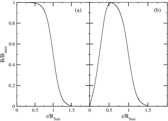
Figure 1: Magnetic field profiles: (a) Wood-Saxon shape; (b) Gaussian shape

In our analysis, we used two types of magnetic profiles.

First, we took the magnetic field profile to be a Wood-Saxon shape of the form

$$B(r)=\frac{B_{0}}{1+\exp[10(r-R_{\odot})/R_{\odot}]}$$ (7)

where $B_{0}$ is the strength of the magnetic field at the center of the Sun.

The second magnetic field profile that we used is a Gaussian shape. Altough there are many other profiles $\left[14,17-19,21,23\right]$ we considered only those two as typical for our purpose as shown figure 1. The effects of these different profiles have been discussed in the conclusion section.

4. Statistical Analysis

In the literature, there is a common way often called $\chi^{2}$ analysis to find the values of the neutrino oscillation parameters $\Delta m^{2}$, $\tan^{2}\theta$ and to calculate the confidence levels of allowed regions and the goodness of a fit $\left[33-36\right]$. In our analysis, we use ”covariance approach” to find the allowed regions mentioned above. By this method, one minimizes the least-squares function

$$\chi_{{}_{\odot}}^{2}=\sum_{i_{1},i_{2}}^{N_{\exp}}(R_{i_{1}}^{(\exp)}-R_{i_{1}}^{(thr)})(V^{-1})_{i_{1}i_{2}}(R_{i_{2}}^{(\exp)}-R_{i_{2}}^{(thr)})$$ (8)

where $V^{-1}$ is the inverse of the covariance matrix of experimental and theoretical uncertainties, $R_{i}^{(\exp)}$ is event rate calculated in the $i$th experiment and $R_{i}^{(thr)}$ is the theoretical event rate for $i$th experiment. The indices indicate the solar neutrino experiments: $i,i_{1},i_{2}=1,...,N_{\exp}$ with $N_{\exp}=4$.

$$V_{i_{1}i_{2}}=V_{i_{1}i_{2}}(\exp)+V_{i_{1}i_{2}}(thr)$$ (9)

$$V_{i_{1}i_{2}}(\exp)=\delta_{i_{1}i_{2}}\sigma_{i_{1}}^{\exp}\sigma_{i_{2}}^{\exp}$$ (10)

where $\sigma_{i}^{\exp}$ are the experimental uncertainties for $i$th experiment.

$$V_{i_{1}i_{2}}(thr) =\delta_{i_{1}i_{2}}\sum_{j_{1}=1}^{8}R_{j_{1}i_{1}}^{(thr)^{2}}\Delta\ln C_{j_{1}i_{1}}^{(thr)^{2}}+$$ (11)

$$\sum_{j_{1},j_{2}=1}^{8}R_{j_{1}i_{1}}^{(thr)^{2}}R_{j_{2}i_{2}}^{(thr)^{2}}\sum_{k=1}^{12}\alpha_{j_{1}k}\alpha_{j_{2}k}(\Delta\ln X_{k})^{2}$$

where the indices $j_{1}$,$j_{2}=1,...,8$ indicate solar neutrino fluxes produced in the eight thermonuclear reactions in the Sun: pp, pep, hep, ⁷Be, ⁸B, ¹³N, ¹⁵O, ¹⁷F, respectively. The index k=1,…,12 denotes the input astrophysical parameters $X_{k}$ in the Standard Solar Model(SSM), on which SSM neutrino fluxes $\Phi_{j}^{SSM}$ depend. The logarithmic derivatives

$$\alpha_{jk}=\frac{\partial\ln\Phi_{j}^{SSM}}{\partial\ln X_{k}}$$ (12)

govern the uncertainties of the neutrino fluxes $\Phi_{j}^{SSM}$. $\Delta\ln X_{k}$ and $\Delta\ln C_{ji}^{(thr)}$ are 1$\sigma$ relative uncertainties of SSM input parameters and the energy-averaged cross section( $C_{ji}^{(thr)}$), respectively.

Theoretical event rates for the radio-chemical experiments, chlorine experiments(Homestake) and gallium experiments(SAGE,GALLEX,GNO), can be found as

$$R_{ij}^{(thr)}=\int dE\phi_{i}\left(E\right)\sigma_{j}(E)P_{ij}(\nu_{e}\rightarrow\nu_{e},E)$$ (13)

such that

$$R_{j}^{(thr)}=\sum_{i=1}^{8}R_{ij}^{(thr)}$$ (14)

where $\phi_{i}\left(E\right)$ is the flux at energy E coming from $i$th reaction and $\sigma_{j}(E)$ is the cross section for detector j.

Solar neutrinos are observed in SK via the Cerenkov light from the neutrino-electron scattering (ES) reaction:

$$\nu_{x}+e^{-}\rightarrow\nu_{x}+e^{-}$$

where $\nu_{x}$ can be $\nu_{e}$ or $\nu_{\mu}$.

Since SNO is heavy water-Cerenkov detector, it observes solar neutrinos by charged-current(CC) and neutral-current(NC) in addition to ES

$$\nu_{e}+d \rightarrow p+p+e^{-}\text{ \ \ \ \ \ \ \ \ \ \ \ \ \ }(CC)$$

$$\nu_{x}+d \rightarrow n+p+\nu_{x}\text{ \ \ \ \ \ \ \ \ \ \ \ \ \ }(NC)$$

The  Cerenkov light is generated by recoiling electron from the ES and CC reactions.

Because of higher threshold energy of SK and SNO experiments($T_{threshold}>5$ $MeV$), they are sensitive to only ⁸B and hep neutrinos. Due to the small flux of hep neutrinos we completely neglect its contribution to the total rates.

For SK and SNO, the theoretical event rates from ES:

$$R_{SK}^{ES} =\int dE\phi_{i}\left(E\right)\{\sigma_{\nu_{e}}^{{}_{j}}(E)P_{j}(\nu_{e}\rightarrow\nu_{e},E,t)+$$ (15)

$$\text{ \ \ \ \ \ \ \ \ \ \ \ \ \ \ \ \ \ \ }\sigma_{\nu_{x}}^{{}_{j}}(E)\left[1-P_{j}(\nu_{e}\rightarrow\nu_{e},E,t)\right]\}$$

where

$$\sigma_{\nu_{e}(\nu_{x})}^{{}_{j}}(E)=\int_{T_{\min}}^{T_{\max}}\frac{d^{2}\sigma}{dTdE}dT$$ (16)

Here $T$ is the kinetic energy of the recoiling electron. $T_{\min}=E_{threshold}-m_{e}$ with $E_{threshold}=5.5$ MeV and $T_{\max}=2E/(2E+m_{e})$ are the minimum and maximum kinetic energy of the recoiling electron, respectively. The differantial cross sections for $\nu_{e}-e^{-}$ and $\nu_{x}-e^{-}$ scatterings are $[37]$

$$\frac{d^{2}\sigma}{dTdE}=\sigma_{e}[g_{L}^{2}+g_{R}^{2}(1-T/E)^{2}-g_{L}g_{R}(T/E^{2})]$$ (17)

with

$$g_{L}=(\pm\frac{1}{2}+\sin^{2}\theta_{W})\text{ \ \ \ \ \ \ }g_{R}=\sin^{2}\theta_{W}\text{\ \ \ \ \ \ \ \ }$$

The upper sign is for $\nu_{e}-e^{-}$ scattering and the lower sign for $\nu_{x}-e^{-}$ scattering; x can be $\mu$ or $\tau.$ The cross section factor is

$$\sigma_{e}=\frac{2G_{F}^{2}m_{e}^{2}}{\pi h^{4}}=88.083\times 10^{-46}cm^{2}$$

For SNO, in addition to the ES, the theoretical event rates come from the CC and NC reactions

$$R^{CC} =\int dE\phi_{i}\left(E\right)\sigma_{CC}^{{}_{j}}(E)P_{j}(\nu_{e}\rightarrow\nu_{e},E,t)$$ (18)

$$R^{NC} =\int dE\phi_{i}\left(E\right)\sigma_{NC}^{{}_{j}}(E)$$ (19)

Total event rates are

$$R^{SNO}=R^{CC}+R^{NC}$$

Because of its substantially lower cross section compered to the other two reactions’, we don’t take into account $R^{ES}$.

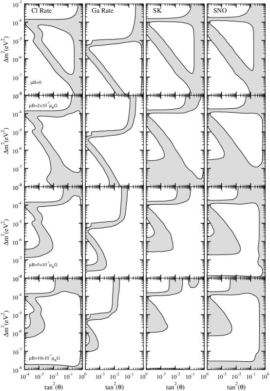
Figure 2: The allowed regions of neutrino parameter space for each solar neutrino experiment seperately at $\mu B=0,2,5,10\times 10^{-7}\mu_{B}G$ and at 95% CL. Each column and row are for the same experiment and at the same $\mu B$ value,respectively(e.g. in the second row at third column, an allowed region for SK experiment at $\mu B=2\times 10^{-7}\mu_{B}G$ is seen)

We took fluxes and cross sections for event rates and error matrixes from Bahcall $[37$, homepage$]$.

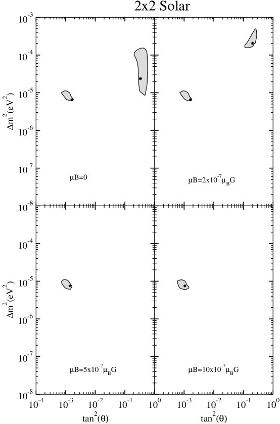
Figure 3: The allowed regions from combined solar neutrino experiments( chlorine, all three gallium, SK and SNO experiments) at the same $\mu B$ values and CL as in figure 2. Stars indicate the local best-fit points.

We need to calculate $\chi_{KamLAND}^{2}$ for the global analysis

$$\chi_{gl}^{2}=\chi_{{}_{\odot}}^{2}+\chi_{{}_{KamLAND}}^{2}$$ (20)

For this purpose we note that, the goal of the KamLAND is to search for antineutrinos emitted from distant power reactor through the reaction

$$p+\overline{\nu}_{e}\rightarrow n+e^{+}$$ (21)

As in $[38]$, the antineutrinos’ energy spectrum is given by

$$\frac{dN_{\overline{\nu}_{e}}^{j}}{dE}\propto\exp(a_{0}+a_{1}E+a_{2}E^{2})$$ (22)

where $j=1,2,3,4$ corresponding to the four isotopes ²³⁵U, ²³⁹P, ²³⁸U, ²⁴¹Pu and the fitted values of the $a_{k}$ are given in detail in $[39]$ for each isotope.

In the case of two generations, the survival probability for the electron antineutrinos coming from the j^th reactor

$$P(\overline{\nu}_{e}\rightarrow\overline{\nu}_{e})=1-\sin^{2}2\theta\sin^{2}(\frac{1.27\Delta m^{2}(eV^{2})d_{j}(km)}{E(GeV)})$$ (23)

here $d_{j}$ is the reactor-detector distance. The number of expected events for each bin at KamLAND is

$$N_{i}^{thr}(t,E,\Delta m^{2},\sin^{2}2\theta) =\eta N_{p}{\displaystyle\int}dE_{V}{\displaystyle\int}dE_{e}R(E_{V},E_{e})\times$$ (24)

$$\text{ \ \ \ \ \ \ }\sum_{j}\frac{S_{j}}{4\pi d_{j}^{2}}\sigma(E_{\nu})P(\overline{\nu}_{e}\rightarrow\overline{\nu}_{e},E_{\nu})$$

here $N_{p}$ is the number of free protons in the fiducial volume of detector and $\eta$ is the efficiency which are given in $[24]$. $S_{j}$ is the initial energy spectrum of reactor $j$ calculated using the thermal power and the isotropic composition of each detector that is given in detailed in $[39]$ and $\sigma(E_{\nu})$ is the lowest cross section

$$\sigma(E_{\nu})=\frac{2\pi^{2}}{m_{e}^{5}f\tau_{n}}p_{e}E_{e}$$ (25)

where $f=1.69$ is the integrated Fermi function for neutron, $m_{e}$ is the positron mass, $\tau_{n}$ is the neutron lifetime, $p_{e}$ and $E_{e}$ are the positron momentum and energy, respectively. So that we have

$$E_{e}=E_{\nu}-1.293\text{ MeV}$$ (26)

The energy resolution function $R(E_{V},E_{e})$ which depends on visible energy $\left(E_{V}\right)$ and true positron energy $\left(E_{e}\right)$ is given by

$$R(E_{V},E_{e})=\frac{1}{\sqrt{2\pi\sigma_{0}^{2}}}e^{-\frac{\left(E_{V}-E_{e}+m_{e}\right)^{2}}{2\sigma_{0}^{2}}}$$ (27)

in which $E_{V}=E_{e}+m_{e}$ and $\sigma_{0}=6.2\%\sqrt{E_{e}}$ $[24]$.

The new KamLAND data results were reported at $[24]$ in 13 bins above the threshold which is 2.6 MeV. To find $\chi^{2}$ for KamLAND spectrum data, due to the low statistics, we use $\chi^{2}$ assuming a Poisson distribution given by

$$\chi_{KL-Spect}^{2}=\underset{i}{\mathop{\displaystyle\sum}}\left[2\left(\kappa N_{i}^{thr}-N_{i}^{\exp}\right)+2N_{i}^{\exp}\ln(\frac{N_{i}^{\exp}}{\kappa N_{i}^{thr}})\right]+\frac{(\kappa-1)^{2}}{\sigma_{sys}^{2}}$$ (28)

where sum is over the KamLAND spectral bins, $\sigma_{sys}^{2}$ is the systematic uncertainty taken to be $6.5\%$ and $\kappa$ is allowed to vary freely.

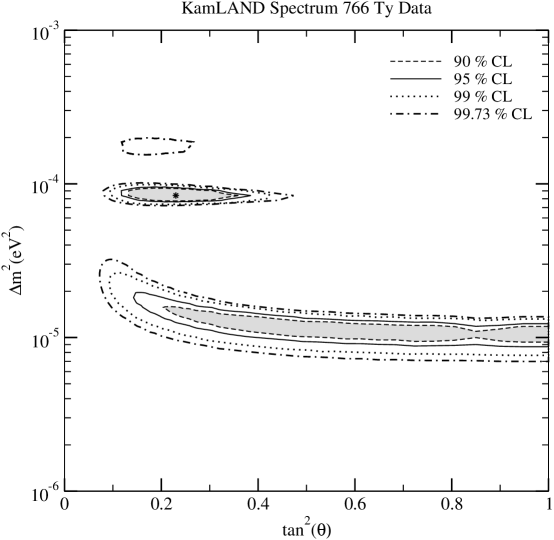
Figure 4: Allowed regions from the new KamLAND spectrum at different confidence levels. The star indicates the best fit point.

5.Results and conclusions

In our calculations, we assumed that the magnetic field extends over the entire Sun for either Wood-Saxon shape or Gaussian shape. We use the neutrino spectra from the Standard Solar Model of Bahcall and his collaborators $\left[40\right]$. In our analysis we calculated allowed regions at 95% confidence level.

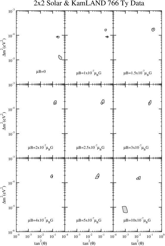
Figure 5: Allowed regions from the combined solar+new KamLAND spectral analysis at different $\mu B$ values and at 95% CL. Stars indicate the best fit points.

We first considered only solar neutrino data. In our statistical analysis, we used the covariance approach. We show the allowed regions of neutrino parameter space in figure 2 for each solar neutrino experiment seperately at four $\mu B$ values using Wood-Saxon field profiles. In figure 2 each column and row are for the same experiment and at the same $\mu B$ value respectively(e.g. in the second row at the third column, an allowed region for SK experiment at $\mu B=2\times 10^{-7}\mu_{B}G$ is seen).

In figure 3, we displayed the allowed regions from combined solar neutrino experiments at the same values of $\mu B$ in figure 2.

After we investigated the combined solar data at different $\mu B$ values, we looked for allowed regions at different confidence levels from new binned KamLAND data $[24]$ in figure 4. We show the allowed regions from our global analysis combining solar and new KamLAND data in figure 5 for nine different $\mu B$ values($0,1,1.5,2,2.5,3,4,5,10\times 10^{-7}\mu_{B}G$ ). In that figure, our results showed that the allowed regions in the LMA shifted to the SMA region as $\mu B$ value is increased. This shift enables us to put an upper limit on the value of $\mu B$ , since the latest experimental data prominently indicate the LMA region (namely excluding SMA and the others).

Table1. Best fit points of global analysis for both magnetic field profiles.

$\mu B$ $($ $\times 10^{-7}$ $\mu_{B}G)$	$\Delta m^{2}(eV^{2})$	tan${}^{2}\theta$	($\chi_{\min}^{2}$)Wood-Saxon	($\chi_{\min}^{2}$)Gaussian
0	8.7$\times 10^{-5}$	0.26	26.38	26.38
1	8.7$\times 10^{-5}$	0.33	35.4	35.64
1.5	1.77$\times 10^{-4}$	0.20	38.6	38.8
2	1.77$\times 10^{-4}$	0.16	41.13	41.16
2.5	1.77$\times 10^{-4}$	0.13	43.81	44.02
3	1.77$\times 10^{-4}$	0.095	42.47	42.92
4	1.77$\times 10^{-4}$	0.095	42.59	42.45
5	1.77$\times 10^{-4}$	0.057	49.39	49.73
7	1.53$\times 10^{-4}$	0.022	53.78	54.13
10	1.53$\times 10^{-4}$	0.012	55.5	55.85

We next calculated the global analysis again for a magnetic profile of Gaussian-shape to show how the magnetic profile in the sun effects the allowed regions and the minimum chi-squares. The results of our global analysis for both magnetic field profiles are given in table 1. As can be seen from the table there are no appreciable differences between the effects of the two magnetic field profiles on the allowed regions and chi-squares values.

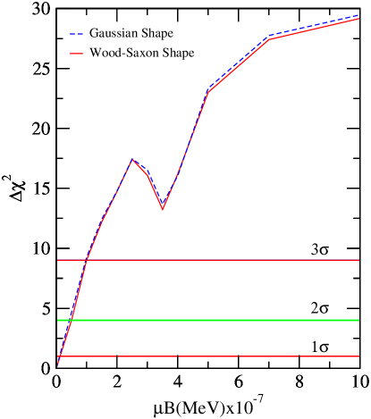
Figure 6: Projection of the global $\Delta\chi^{2}$ function on $\mu B$. The solid line and short-dashed lines represent the calculation using Wood-Saxon shape of magnetic profile and Gaussian shape of magnetic profile, respectively.

Finally in figure 6 we present projection of the global $\Delta\chi^{2}$ function on the $\mu B$  to place a limit on $\mu B$ for the two magnetic field profiles. From this figure we found a general limit, since the graphes for the two magnetic profiles almost coincide: $\mu B<$ $0.2\times 10^{-7}\mu_{B}G$, $0.5\times 10^{-7}\mu_{B}G$, $1.0\times 10^{-7}\mu_{B}G$ for $1\sigma,2\sigma,3\sigma$ limit, respectively. On the other hand there is intensive work related to the electromagnetic properties of the neutrinos. Since neutrinos are known to be massive they can get tiny magnetic moments even in the SM also in its extensions. Astrophysical considerations $[41]$ put strong constraints on the magnetic moment of the neutrinos as $\mu_{\nu}<10^{-12}\mu_{B}$, however these bounds are model dependent. Also the reactor experiments bring less restrictive limits of $\mu_{\nu}<1.3\times 10^{-10}\mu_{B}$ $[42,43]$. An analysis of the Super-Kamiokande solar neutrino data $[44]$ enables the authors to put again a similar limit of $\mu_{\nu}<1.5\times 10^{-10}\mu_{B}$. As for the magnetic field of the Sun, from the existing observations an upper limit of $10^{7}G$ at the core and a maximum magnitude of $3\times 10^{5}G$ at the bottom of the convective zone are usually taken in the literature [21, 22]. Hence the above restriction according to our analysis on the $\mu B$ value agrees with the present limits of $\mu_{\nu}$ and $B_{Sun}$.

Also the consideration of the two magnetic field profiles seem to be satisfactory at this level, because there are no differences between their effects on the allowed regions and the chi-square values for both of them. Actually the whole analysis can be repeated for many other field profiles $[14,17-19,21,23]$ in order to better investigate the detailed behaviour of the magnetic field in the Sun. This could be a topic of a future work.

Acknowledgments

We would like to thank to Prof.Dr. A. Baha Balantekin for his suggestion of this research topic and for his kind help. We are gratefull to the referees for their clarifying suggestions. One of the authors, D. Yilmaz, also thanks TUBITAK (The Scientific and Technical Research Council of Turkey) for the grant given to support his research at University of Wisconsin-Madison.

References

$\left[1\right]$   Cleveland B T et al 1998 Astrophys. J. 496 505

$\left[2\right]$   Abdurashitov J N et al (SAGE Collaboration) 2002 J. Exp. Theor. Phys. 95 181

Abdurashitov J N et al 2002 Zh. Eksp. Teor. Fiz. 122 211 (Preprint astro-ph/0204245)

$\left[3\right]$   Hampel W et al (GALLEX Collaboration) 1999 Phys. Lett. B 447 127

$\left[4\right]$   Altmann M et al (GNO Collaboration) 2000 Phys. Lett. B 490 16 (Preprint hep-ex/0006034)

$\left[5\right]$ Bahcall J N, Huebner W F, Lubow S H, Parker P D , and Ulrich R K , Rev. Mod. Phys. 54, 767 (1982)

$\left[6\right]$ Wolfenstein L, Phys. Rev. D 17, 2369 (1978) ; 20, 2634 (1979).

$\left[7\right]$ Mikheyev S P and Smirnov A Yu , Nuovo Cimento C 9, 17 (1986) ; Yad. Fiz. 42, 1441 (1985) ; [Sov. J. Nucl. Phys. 42, 913 (1985)].

$\left[8\right]$ Okun L B, Voloshin M B, and Vysotsky M I, Yad. Fiz. 44, 677 (1986) ; [Sov. J. Nucl. Phys. 44, 440 (1986)].

$\left[9\right]$ Akhmedov E Kh , Phys. Lett. B 213, 64 (1988); E. Kh. Akhmedov and M. Yu. Khlopov, Mod. Phys. Lett. A 3, 451 (1988).

$\left[10\right]$ Barbieri R and Fiorentini G, Nucl. Phys. B 304, 909 (1988).

$\left[11\right]$ Bethe H A, Phys. Rev. Lett. 63, 837 (1989) .

$\left[12\right]$ Lim C S and Marciano W J, Phys. Rev. D 37, 1368 (1988)

$\left[13\right]$ Balantekin A B, Hatchell P J, Loreti F, Phys. Rev. D 41 3583 (1990)

$\left[14\right]$ Pulido J, 2002 A. High Energy Phys. AHEP2003/046

$\left[15\right]$ Chauhan C B, Pulido J, 2004 Preprint hep-ph/0402194

$\left[16\right]$ Lim C S, 2001 Kashiwa 2001, Neutrino Oscillation and Their Origin 64

$\left[17\right]$ Chauhan C B, Pulido J, 2002 Preprint hep-ph/0206193

$\left[18\right]$ Chauhan C B, 2002 Preprint hep-ph/0204160

$\left[19\right]$ Bykov A A, Popov V Y, Rashba T I, Semikoz V B, 1999 Preprint hep-ph/0002174

$\left[20\right]$ Derkaoui J, Tayalati Y, 1999 Preprint hep-ph/9909512

$\left[21\right]$ Akhmedov E Kh, Pulido J, 1999 Preprint hep-ph/9907399

$\left[22\right]$ Akhmedov E Kh, Pulido J, 2002 Preprint hep-ph/0209192

$\left[23\right]$ Chauhan C B, Pulido J, Torrente-Lujan E, 2003 Preprint hep-ph/0304297

$\left[24\right]$   Araki T et al (KamLAND Collaboration) 2004 Preprint hep-ph/0406035

$\left[25\right]$   Ahmad Q R et al (SNO Collaboration) 2001 Phys. Rev. Lett. 87 071301 (Preprint nucl-ex/0106015)

$\left[26\right]$   Ahmad Q R et al (SNO Collaboration) 2002 Phys. Rev. Lett. 89 011301 (Preprint nucl-ex/0204008)

$\left[27\right]$   Fukuda S et al (Super-Kamiokande Collaboration) 2001 Phys. Rev. Lett. 86 5651 (Preprint hep-ex/0103032)

Fukuda S et al (Super-Kamiokande Collaboration) 2001 Phys. Rev. Lett. 86 5656 (Preprint hep-ex/0103033)

$\left[28\right]$   Bahcall J N, Gonzalez-Garcia M C and Pena-Garay C 2002 J. High Energy Phys. JHEP 07(2002)054 (Preprint hep-ph/0204314)

$\left[29\right]$ Eguchi K et al (KamLAND Collaboration) 2002 Preprint hep-ex/0212021.

$\left[30\right]$ Balantekin A B, Fricke S H , and Hatchell P J, Phys. Rev. D 38, 935 (1988) .

$\left[31\right]$ Voloshin M B , Pis’ma Zh. Eksp. Teor. Fiz. 47, 421 (1988) ; [JETP Lett. 47, 501 (1988)]; Phys. Lett. B 209, 360 (1988).

$\left[32\right]$ M. Leurer and J. Liu, Phys. Lett. B 219, 304 (1989).Giuliani and S. Ranfone, Nucl. Phys. B325, 724 (1989).

$\left[33\right]$ Feldman G J and Cousins R D 1998 Phys. Rev. D 57 3873 (Preprint physics/9711021)

$\left[34\right]$ Fogli G L, Lisi E, Marrone A, Montanino D and Palazzo A 2002 Phys. Rev. D 66 053010 (Preprint hep-ph/0206162)

$\left[35\right]$ Garzelli M V and Giunti C 2002 Astropart. Phys. 17 205 (Preprint hep-ph/0007155)

Garzelli M V and Giunti C 2002 Phys. Rev. D 65 093005 (Preprint hep-ph/0111254)

Garzelli M V and Giunti C 2001 J. High Energy Phys. JHEP12(2001)017 (Preprint hep-ph/0108191)

$\left[36\right]$ Gonzalez-Garcia M C and Nir Y 2002 Preprint hep-ph/0202058

$\left[37\right]$ Bahcall J N 1989 Neutrino Astrophysics (Cambridge: Cambridge University Press)

$\left[38\right]$ Murayama H and Pierce A, Phys. Rev. D 65 013012 (Preprint hep-ph/0012075)

$\left[39\right]$ Bandyopadhyay A, Choubey S, Goswami S, Gandhi R, Roy D P, J. Phys. G 29, 665 (2003)

$\left[40\right]$   Bahcall J N, Pinsonneault M H and Basu S 2001 Astrophys. J. 555 990 (Preprint astro-ph/0010346)

$\left[41\right]$   Raffelt G G 1990 Phys. Rev. Lett. 64 2856; 1999 Phys. Rep. 320 319; Castellani V, Degl’Innocenti S 1993 Astrophys. J. 402 574

$\left[42\right]$   MUNU Collaboration 2002 Preprint hep-ex/0304011

$\left[43\right]$   Li H B et al 2003 Phys. Rev. Lett. 90 131802

$\left[44\right]$   Beacom J F, Vogel P 1999 Phys. Rev. Lett. 83 5222