Correlation of small–x gluons
in impact parameter space

Abstract

In the framework of the QCD dipole model at high energy, we present an analytic evaluation of the dipole pair density in two limits in which the parent dipole is much larger/smaller than the distance between the two child dipoles. Due to conformal symmetry, the two limits give an identical result. The power–law correlation between dipoles explicitly breaks the factorization of target–averaged scattering amplitudes.

1 Introduction

A hadron in the infinite momentum frame is a complicated system of small–x gluons. While the energy evolution of the average gluon number can be described by the Balitsky–Fadin–Kuraev–Lipatov (BFKL) equation [1], the wavefunction of a hadron contains more information than just the average number. For example, the fluctuation of the gluon number plays a crucial role in the evolution of scattering amplitudes towards the unitarity limit, and has recently attracted considerable interest [2, 3, 4, 5, 6, 7, 8, 9] in the context of saturation physics [10, 11, 12].

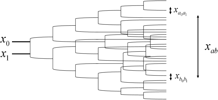
Another important characteristic of the hadron wavefunction is the correlation of gluons in the impact parameter space. In the dilute, non–saturated regime, soft gluons are necessarily correlated because they originate from a common ancestor via gluon splitting. The process can be most easily described in the QCD dipole model formulated in the large $N_{c}$ approximation [14, 15, 16]. In this approach, the evolution of the ‘parent’ dipole (a quark–antiquark pair) proceeds via dipole splitting with certain probability computed in perturbation theory (Fig. 1). Since the probability depends nontrivially on transverse coordinates, ‘child’ dipoles will be distributed in the transverse plane with characteristic correlations between them. Although this dynamics is built–in in the numerical Monte–Carlo simulation of this model [2, 17], so far there have been only few analytical insights [15, 16, 18, 19]. (See, also, [20].) In this paper we evaluate the dipole pair density in certain limits and find the power–law correlation between dipoles at large distances with the power determined by the conformal weights of the BFKL eigenfunction [21]. As an immediate consequence of our result, we shall show in Eqs. (3.18) and (4.21) that the factorization of dipole scattering amplitudes is explicitly violated by a position–dependent multiplicative factor

$$\langle T_{1}T_{2}\rangle\approx c_{12}\langle T_{1}\rangle\langle T_{2}\rangle\qquad c_{12}\gg 1,$$ (1.1)

where $T$ is the single dipole scattering amplitude and $\langle...\rangle$ denotes the averaging over the target wavefunction. Eq. (1.1) should be contrasted with the fact that scattering amplitudes computed in the BK–JIMWLK framework [13] essentially factorize

$$\langle T_{1}T_{2}\rangle\approx\langle T_{1}\rangle\langle T_{2}\rangle+{\cal O}\left(\frac{1}{N_{c}^{2}}\right).$$ (1.2)

The gluon splitting diagrams which lead to Eq. (1.1) are not included in the BK–JIMWLK equation which rather sums gluon recombination diagrams. Thus it is not surprising that the factorization in Eq. (1.2) does not hold for a more general evolution. While Eq. (1.2) may be valid if one starts with a large nucleus with totally uncorrelated partons [12] and follows the BK–JIMWLK evolution up to not so high energies, it is likely that the correlation in the transverse plane developed in the dilute regime significantly affects the nonlinear evolution of hadrons as in the case of the gluon number fluctuation [3, 4, 5, 6, 7, 8].

Figure 1: A cascade of dipole splitting. Thin lines represent child dipoles produced by the parent dipole $(x_{0},x_{1})$.

2 Single dipole density

In this section, we review the properties of the single dipole distribution. The techniques used here can be directly applied to the analysis of the dipole pair density in the next section. The single dipole density evolved up to rapidity $Y$ is given by

$$n_{Y}(x_{01},x)=2\frac{x_{01}^{2}}{x^{2}}\int\frac{d\gamma}{2\pi i}e^{\chi(\gamma)Y-\gamma\ln\frac{x_{01}^{2}}{x^{2}}},$$ (2.1)

$x_{01}=x_{0}-x_{1}$ and $x\equiv x_{23}=x_{2}-x_{3}$ denote the coordinates of the parent dipole and the child dipole, respectively. We shall use the letter $x$ for two–dimensional real vectors and $z$ for corresponding complex coordinates. By slight abuse of notation, we use $x$ also for the magnitude of two dimensional vectors. $\chi$ is the usual BFKL eigenvalue

$$\chi(\gamma)=2\bar{\alpha}_{s}\mbox{Re}\{\psi(1)-\psi(\gamma)\}.$$ (2.2)

The saddle point of the $\gamma$–integral is given by

$$\chi^{\prime}(\gamma)Y=\ln\frac{x_{01}^{2}}{x^{2}}$$ (2.3)

When $x_{01}>x$, the saddle point is in the region $1>\gamma>\frac{1}{2}$, and

$$n_{Y}(x_{01},x)\sim e^{\chi(\gamma)Y}\left(\frac{x_{01}^{2}}{x^{2}}\right)^{1-\gamma}.$$ (2.4)

$n$ is proportional to the scattering amplitude between dipoles of sizes $x_{01}$ and $x$.

$$T_{Y}(x_{01},x)=\frac{\pi\alpha_{s}^{2}x^{2}}{2\gamma^{2}(1-\gamma)^{2}}n_{Y}(x_{01},x)$$ (2.5)

Eq. (2.1) is integrated over the impact parameter $b\equiv\frac{x_{2}+x_{3}}{2}-\frac{x_{0}+x_{1}}{2}$ between the parent and child dipoles . The $b$–dependent distribution is

$$n_{Y}(x_{01},x,b)=\frac{16}{x^{2}}\sum_{n}\int\frac{d\nu}{(2\pi)^{3}}(\nu^{2}+\frac{n^{2}}{4})\,e^{\chi(n,\nu)Y}$$

$$\quad\times\int d^{2}\omega E^{1-h,1-\bar{h}}(b+\frac{x}{2}-\omega,b-\frac{x}{2}-\omega)E^{h,\bar{h}}(\frac{x_{01}}{2}-\omega,-\frac{x_{01}}{2}-\omega).$$ (2.6)

$E$ is the eigenfunction of the SL(2,C) group

$$E^{h,\bar{h}}(x_{0\gamma},x_{1\gamma})=(-1)^{n}\left(\frac{z_{01}}{z_{0\gamma}z_{1\gamma}}\right)^{h}\left(\frac{\bar{z}_{01}}{\bar{z}_{0\gamma}\bar{z}_{1\gamma}}\right)^{\bar{h}},$$

$$E^{h,\bar{h}*}(x_{0\gamma},x_{1\gamma})=E^{1-h,1-\bar{h}}(x_{0\gamma},x_{1\gamma})$$ (2.7)

with $h=\frac{1-n}{2}+i\nu$, $\bar{h}=\frac{1+n}{2}+i\nu=1-h^{*}$. Eq. (2.1) is obtained from Eq. (2.6) by integrating over $b$

$$n_{Y}(x_{01},x)=\int d^{2}b\ n_{Y}(x_{01},x,b),$$ (2.8)

keeping only the $n=0$ term and identifying $h=\frac{1}{2}+i\nu\equiv\gamma$. The $w$–integral in Eq. (2.6) has been carried out in [22, 23]. Due to global conformal symmetry, the result depends only on the anharmonic ratio

$$\rho\equiv\frac{z_{01}z}{z_{02}z_{13}},$$ (2.9)

The $n=0$ term gives,

$$n_{0\nu}(x_{01},x,b)\equiv\frac{2\nu^{2}}{x^{2}\pi^{4}}\Bigl{(}b_{0,\nu}|\rho|^{2(1-\gamma)}F(1-\gamma,1-\gamma,2(1-\gamma);\rho)F(1-\gamma,1-\gamma,2(1-\gamma);\bar{\rho})$$

$$+b^{*}_{0,\nu}|\rho|^{2\gamma}F(\gamma,\gamma,2\gamma;\rho)F(\gamma,\gamma,2\gamma;\bar{\rho})\Bigr{)},$$ (2.10)

where $F$ is the hypergeometric function and

$$b_{0,\nu}=\pi^{3}\frac{2^{4i\nu}}{i\nu}\frac{\Gamma(\frac{1}{2}-i\nu)\Gamma(1+i\nu)}{\Gamma(\frac{1}{2}+i\nu)\Gamma(1-i\nu)}.$$ (2.11)

Consider the case $x_{01}\gg x$ and look at the region of small impact parameters $x_{01}\gg b$. In this region,

$$\rho\approx\frac{-4z}{z_{01}},\qquad|\rho|\ll 1,$$ (2.12)

and one may approximate $F(...;\rho)\approx 1$. We obtain

$$n_{Y}(x_{01},x,b)=\int\frac{d\nu}{2\pi}n_{0,\nu}(x_{01},x,b)e^{\chi(0,\nu)Y}\approx\frac{1}{x_{01}^{2}}\int d\nu e^{\chi(0,\nu)Y}\frac{16^{\gamma}\nu^{2}b_{0,\nu}^{*}}{\pi^{5}}\left(\frac{x^{2}_{01}}{x^{2}}\right)^{1-\gamma}+c.c.$$ (2.14)

Comparing Eq. (2.1) and Eq. (2.14), one sees that in the saddle point approximation,

$$n_{Y}(x_{01},x)\sim x_{01}^{2}\,n_{Y}(x_{01},x,b\ll x_{01}).$$ (2.15)

Therefore, roughly child dipoles are uniformly distributed inside the area $x_{01}^{2}$ (c.f., Eq. (2.8)). On the other hand, the dipole density at large impact parameters $b\gg x_{01}$ are suppressed. Indeed, in this region, $\rho\approx\frac{z_{01}z}{b^{2}}$, and

$$n_{Y}(x_{01},x,b)\approx\frac{1}{x^{2}}\int d\nu\frac{\nu^{2}b_{0,\nu}^{*}}{\pi^{5}}\left(\frac{x_{01}^{2}x^{2}}{b^{4}}\right)^{\gamma}e^{\chi(0,\nu)Y}+c.c..$$ (2.16)

At the saddle point, $n(b)\sim 1/b^{4\gamma}$ where $\gamma$ is determined from $\chi^{\prime}(\gamma)Y=\ln\frac{b^{4}}{x_{01}^{2}x^{2}}$.

Let us compare this $b$–dependence with that of the saturation momentum. The dipole–dipole scattering amplitude at a fixed impact parameter $b$ is

$$T_{Y}(x_{01},x,b)=\int d^{2}b^{\prime}\frac{d^{2}x^{\prime}}{2\pi x^{\prime 2}}A_{0}(x,x^{\prime},b-b^{\prime})n_{Y}(x_{01},x^{\prime},b^{\prime}),$$ (2.17)

where $A_{0}$ is the dipole–dipole scattering amplitude in the two–gluon exchange approximation. Since $A_{0}(b-b^{\prime})$ decays like $1/(b-b^{\prime})^{4}$, one may approximate

$$T_{Y}(x_{01},x,b)\approx\int d^{2}b^{\prime}A_{0}(x,x^{\prime},b-b^{\prime})\int\frac{d^{2}x^{\prime}}{2\pi x^{\prime 2}}n_{Y}(x_{01},x^{\prime},b)$$

$$=\pi\alpha_{s}^{2}\int\frac{d^{2}x^{\prime}}{2\pi x^{\prime 2}}r^{2}_{<}(1+\ln\frac{r_{>}}{r_{<}})n_{Y}(x_{01},x^{\prime},b)$$ (2.18)

where $r_{<}=\mbox{min}\{x,x^{\prime}\}$ and $r_{>}=\mbox{max}\{x,x^{\prime}\}$. Using the large $b$ form of $n$, Eq. (2.16), one obtains

$$T_{Y}(x_{01},x,b)\approx\frac{\pi\alpha_{s}^{2}x^{2}}{4\gamma^{2}(1-\gamma)^{2}}n_{Y}(x_{01},x,b).$$ (2.20)

The local ($b$–dependent) saturation momentum can be determined by the constancy of the exponential factor of $T$ in the integral representation along the line $x=1/Q_{s}(b,Y)$ [25, 26], and reads

$$Q^{2}_{s}(b,Y)\sim\frac{x^{2}_{01}}{b^{4}}e^{\frac{\chi(\gamma_{s})}{\gamma_{s}}Y},$$ (2.21)

where $\gamma_{s}\approx 0.628$ solves $\chi^{\prime}(\gamma_{s})=\frac{\chi(\gamma_{s})}{\gamma_{s}}$. Repeating the same procedure for $x_{01}\gg b$, we get

$$Q^{2}_{s}(b,Y)\sim\frac{1}{x_{01}^{2}}e^{\frac{\chi(\gamma_{s})}{\gamma_{s}}Y}.$$ (2.22)

If we take $x$ to be close to the saturation line $\sim 1/Q_{s}(b,Y)$, $\gamma\approx\gamma_{s}$, and the geometric scaling [25, 26, 27] holds locally in the two ($b\gg x_{01}$, $b\ll x_{01}$) regimes [28]

$$T_{Y}(x_{01},x,b)\sim x^{2}n_{Y}(x_{01},x,b)\sim(x^{2}Q_{s}^{2}(b,Y))^{\gamma_{s}}.$$ (2.23)

3 Dipole pair density

In this and the next section, we analyze the dipole pair density $n^{(2)}$ in two different ways. We start with the exact expression for the pair density as derived in [18] (see, also, [29]).

$$n^{(2)}_{Y}(x_{01},x_{a_{0}a_{1}},x_{b_{0}b_{1}})=\int dhdh_{a}dh_{b}\frac{1}{2x^{2}_{a_{0}a_{1}}x_{b_{0}b_{1}}^{2}}\int_{0}^{Y}dy\ e^{\chi(h)y+(\chi(h_{a})+\chi(h_{b}))(Y-y)}$$

$$\times\int d^{2}x_{\alpha}d^{2}x_{\beta}d^{2}x_{\gamma}E^{h,\bar{h}}(x_{0\gamma},x_{1\gamma})E^{h_{a},\bar{h}_{a}}(x_{a_{0}\alpha},x_{a_{1}\alpha})E^{h_{b},\bar{h}_{b}}(x_{b_{0}\beta},x_{b_{1}\beta})$$

$$\times\int\frac{d^{2}x_{2}d^{2}x_{3}d^{2}x_{4}}{x_{23}^{2}x_{34}^{2}x_{42}^{2}}E^{h,\bar{h}*}(x_{2\gamma},x_{3\gamma})E^{h_{a},\bar{h}_{a}*}(x_{2\alpha},x_{4\alpha})E^{h_{b},\bar{h}_{b}*}(x_{3\beta},x_{4\beta}),$$ (3.1)

where $(x_{a_{0}},x_{a_{1}})$ and $(x_{b_{0}},x_{b_{1}})$ are coordinates of the child dipoles of interest. We introduced a compact notation

$$\int dh\equiv\sum_{n}\int d\nu\frac{2\nu^{2}+n^{2}/2}{\pi^{4}}.$$ (3.2)

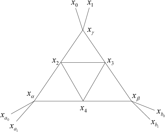
A graphical representation of the coordinate integrals is shown in Fig. 2.

Figure 2: Graphical representation of Eq. (3.1).

We will be interested in configurations where the two child dipoles are small (typically of the order of the inverse saturation scale $\sim 1/Q_{s}$) and far away from each other,

$$x_{ab}=x_{a}-x_{b}\equiv\frac{x_{a_{0}}+x_{a_{1}}}{2}-\frac{x_{b_{0}}+x_{b_{1}}}{2}\gg x_{a_{0}a_{1}},\,x_{b_{0}b_{1}},$$ (3.3)

and try to extract the leading $x_{ab}$ dependence of $n^{(2)}$. This leaves us with two interesting (and in fact, tractable) situations (see, Fig. 3): (A) The parent dipole is also small $x_{01}\sim x_{a_{0}a_{1}},x_{b_{0}b_{1}}\ll x_{ab}$. (B) The parent dipole is large $x_{01}\gg x_{ab}\gg x_{a_{0}a_{1}},x_{b_{0}b_{1}}$.

Figure 3: Case (A): All dipoles are small compared with their mutual separations. Case (B): Child dipoles are deep inside the large parent dipole.

Let us first consider the case A. In the next section we will discuss both cases in a unified way. The last line in Eq. (3.1) is the triple pomeron vertex in perturbative QCD [30] at large $N_{c}$. It has the form

$$f(\bar{h},\bar{h}_{a},\bar{h}_{b})\frac{1}{(z_{\alpha}-z_{\beta})^{1+h-h_{a}-h_{b}}(z_{\beta}-z_{\gamma})^{1+h_{a}-h_{b}-h}(z_{\gamma}-z_{\alpha})^{1+h_{b}-h-h_{a}}}$$

$$\times\frac{1}{(\bar{z}_{\alpha}-\bar{z}_{\beta})^{1+\bar{h}-\bar{h}_{a}-\bar{h}_{b}}(\bar{z}_{\beta}-\bar{z}_{\gamma})^{1+\bar{h}_{a}-\bar{h}_{b}-\bar{h}}(\bar{z}_{\gamma}-\bar{z}_{\alpha})^{1+\bar{h}_{b}-\bar{h}-\bar{h}_{a}}}.$$ (3.4)

This structure follows immediately by noting that the last line of Eq. (3.1) and Eq. (3.4) transform in the same way under the SL(2,C) transformations of $z_{\alpha},\ z_{\beta},\ z_{\gamma}$

$$z\to\frac{\alpha z+\beta}{\gamma z+\delta}\qquad(\alpha\delta-\beta\gamma=1).$$ (3.5)

The function $f(h,h_{a},h_{b})$ can be found in [31, 32]. Next we turn to the remaining integrals $d^{2}x_{\alpha}d^{2}x_{\beta}d^{2}x_{\gamma}$ in (3.1). Since all dipoles (parent, children) are assumed to be very small, typically $x_{0a},\,x_{0b},\,x_{ab}\gg x_{01},\,x_{a_{0}a_{1}},\,x_{b_{0}b_{1}}$ and we may make approximations

$$\left(\frac{z_{01}}{z_{0\gamma}z_{1\gamma}}\right)^{h}\approx\left(\frac{z_{01}}{z^{2}_{0\gamma}}\right)^{h},\ \ \left(\frac{z_{a_{0}a_{1}}}{z_{a_{0}\alpha}z_{a_{1}\alpha}}\right)^{h}\approx\left(\frac{z_{a_{0}a_{1}}}{z^{2}_{a\alpha}}\right)^{h},\ \ \left(\frac{z_{b_{0}b_{1}}}{z_{b_{0}\beta}z_{b_{1}\beta}}\right)^{h}\approx\left(\frac{z_{b_{0}b_{1}}}{z^{2}_{b\beta}}\right)^{h}.$$ (3.6)

We will see later that with this replacement one makes a mistake in the overall factor of $n^{(2)}$ by 8. After this approximation, we are left with the integral

$$\int d^{2}x_{\alpha}d^{2}x_{\beta}d^{2}x_{\gamma}\frac{1}{z^{2h}_{0\gamma}z^{2h_{a}}_{a\alpha}z^{2h_{b}}_{b\beta}}\frac{1}{z_{\alpha\beta}^{1+h-h_{a}-h_{b}}z_{\beta\gamma}^{1+h_{a}-h_{b}-h}z_{\gamma\alpha}^{1+h_{b}-h-h_{a}}}$$

$$\times\frac{1}{\bar{z}^{2\bar{h}}_{0\gamma}\bar{z}^{2\bar{h}_{a}}_{a\alpha}\bar{z}^{2\bar{h}_{b}}_{b\beta}}\frac{1}{\bar{z}_{\alpha\beta}^{1+\bar{h}-\bar{h}_{a}-\bar{h}_{b}}\bar{z}_{\beta\gamma}^{1+\bar{h}_{a}-\bar{h}_{b}-\bar{h}}\bar{z}_{\gamma\alpha}^{\bar{h}_{b}-\bar{h}-\bar{h}_{a}}}.$$ (3.7)

One can check that this integral transforms in the same way under the SL(2,C) transformation of $z_{0},\ z_{a},\ z_{b}$ as

$$\frac{1}{z_{0a}^{h+h_{a}-h_{b}}z_{0b}^{h+h_{b}-h_{a}}z_{ab}^{h_{a}+h_{b}-h}}\frac{1}{\bar{z}_{0a}^{\bar{h}+\bar{h}_{a}-\bar{h}_{b}}\bar{z}_{0b}^{\bar{h}+\bar{h}_{b}-\bar{h}_{a}}\bar{z}_{ab}^{\bar{h}_{a}+\bar{h}_{b}-\bar{h}}}.$$ (3.8)

The coefficient can be easily obtained. In the dominant case of $n=n_{a}=n_{b}=0$ where $h=\bar{h}=\frac{1}{2}+i\nu\equiv\gamma$, $h_{a}=\bar{h}_{a}\equiv\gamma_{a}$, $h_{b}=\bar{h}_{b}\equiv\gamma_{b}$, (Generalization to the case $h\neq\bar{h}$ is straightforward.)

$$\int d^{2}x_{\alpha}d^{2}x_{\beta}d^{2}x_{\gamma}\frac{1}{|z_{0\gamma}|^{4\gamma}|z_{a\alpha}|^{4\gamma_{a}}|z_{b\beta}|^{4\gamma_{b}}}\frac{1}{|z_{\alpha\beta}|^{2(\gamma-\gamma_{a}-\gamma_{b}+1)}|z_{\beta\gamma}|^{2(\gamma_{a}-\gamma_{b}-\gamma+1)}|z_{\gamma\alpha}|^{2(\gamma_{b}-\gamma-\gamma_{a}+1)}}$$

$$=\frac{g(\gamma,\gamma_{a},\gamma_{b})}{|z_{0a}|^{2(\gamma+\gamma_{a}-\gamma_{b})}|z_{0b}|^{2(\gamma+\gamma_{b}-\gamma_{a})}|z_{ab}|^{2(\gamma_{a}+\gamma_{b}-\gamma)}}$$ (3.9)

When $\gamma>1/2$, a pole at $z_{\gamma}=z_{0}$ is not integrable. The following result should be regarded as analytic continuation from convergent values of $\gamma$’s. Using a conformal transformation, one can set $z_{a}=0$, $z_{b}=1$, $z_{0}=\infty$.

$$g(\gamma,\gamma_{a},\gamma_{b})=\int d^{2}x_{\alpha}d^{2}x_{\beta}d^{2}x_{\gamma}\frac{1}{|z_{\alpha}|^{4\gamma_{a}}|1-z_{\beta}|^{4\gamma_{b}}}\frac{1}{|z_{\alpha\beta}|^{2(\gamma-\gamma_{a}-\gamma_{b}+1)}|z_{\beta\gamma}|^{2(\gamma_{a}-\gamma_{b}-\gamma+1)}|z_{\gamma\alpha}|^{2(\gamma_{b}-\gamma-\gamma_{a}+1)}}$$ (3.10)

Evaluating the integrals in the order of $d^{2}x_{\gamma}$, $d^{2}x_{\beta}$ and $d^{2}x_{\alpha}$, one obtains

$$g(\gamma,\gamma_{a},\gamma_{b})=\pi^{3}\frac{\Gamma(1-2\gamma)\Gamma(1-2\gamma_{a})\Gamma(1-2\gamma_{b})\Gamma(\gamma+\gamma_{a}+\gamma_{b}-1)}{\Gamma(2\gamma)\Gamma(2\gamma_{a})\Gamma(2\gamma_{b})\Gamma(2-\gamma-\gamma_{a}-\gamma_{b})}$$

$$\times\frac{\Gamma(\gamma+\gamma_{a}-\gamma_{b})\Gamma(\gamma+\gamma_{b}-\gamma_{a})\Gamma(\gamma_{a}+\gamma_{b}-\gamma)}{\Gamma(1+\gamma_{b}-\gamma_{a}-\gamma)\Gamma(1+\gamma_{a}-\gamma_{b}-\gamma)\Gamma(1+\gamma-\gamma_{a}-\gamma_{b})},$$ (3.11)

and therefore,

$$n^{(2)}=\int d\gamma d\gamma_{a}d\gamma_{b}\frac{1}{2x_{a_{0}a_{1}}^{2}x_{b_{0}b_{1}}^{2}}g(\gamma,\gamma_{a},\gamma_{b})f(\bar{\gamma},\bar{\gamma}_{a},\bar{\gamma}_{b})\int_{0}^{Y}dy\frac{x_{01}^{2\gamma}x_{a_{0}a_{1}}^{2\gamma_{a}}x_{b_{0}b_{1}}^{2\gamma_{b}}\,e^{\chi(\gamma)y+(\chi(\gamma_{a})+\chi(\gamma_{b}))(Y-y)}}{x_{0a}^{2(\gamma+\gamma_{a}-\gamma_{b})}x_{0b}^{2(\gamma+\gamma_{b}-\gamma_{a})}x_{ab}^{2(\gamma_{a}+\gamma_{b}-\gamma)}}$$

$$=\int d\gamma d\gamma_{a}d\gamma_{b}\frac{1}{2x_{a_{0}a_{1}}^{2}x_{b_{0}b_{1}}^{2}}g(\gamma,\gamma_{a},\gamma_{b})f(\bar{\gamma},\bar{\gamma_{a}},\bar{\gamma_{b}})\int_{0}^{Y}dy\,$$

$$\times\exp\left(\chi(\gamma)y+(\chi(\gamma_{a})+\chi(\gamma_{b}))(Y-y)-\gamma\ln\left(\frac{x_{0a}^{2}x_{0b}^{2}}{x_{01}^{2}x_{ab}^{2}}\right)-\gamma_{a}\ln\left(\frac{x_{0a}^{2}x_{ab}^{2}}{x^{2}_{a_{0}a_{1}}x_{0b}^{2}}\right)-\gamma_{b}\ln\left(\frac{x_{0b}^{2}x_{ab}^{2}}{x^{2}_{b_{0}b_{1}}x_{0a}^{2}}\right)\right).$$

The remaining integrals may be evaluated in the saddle point approximation. The saddle points for $y,\ \gamma,\ \gamma_{a,b}$ are given by the solution to

$$\chi(\gamma)=\chi(\gamma_{a})+\chi(\gamma_{b}),$$ (3.13)

$$\chi^{\prime}(\gamma_{a})(Y-y)=\ln\frac{x_{0a}^{2}x_{ab}^{2}}{x_{0b}^{2}x^{2}_{a_{0}a_{1}}}\gg 1,$$ (3.14)

$$\chi^{\prime}(\gamma_{b})(Y-y)=\ln\frac{x_{0b}^{2}x_{ab}^{2}}{x_{0a}^{2}x^{2}_{b_{0}b_{1}}}\gg 1,$$ (3.15)

$$\chi^{\prime}(\gamma)y=\ln\frac{x_{0a}^{2}x_{0b}^{2}}{x_{ab}^{2}x_{10}^{2}}\gg 1,$$ (3.16)

and the dipole pair density behaves like

$$n^{(2)}_{Y}(x_{01},x_{a_{0}a_{1}},x_{b_{0}b_{1}})\sim\frac{e^{(\chi(\gamma_{a})+\chi(\gamma_{b}))Y}}{x_{a_{0}a_{1}}^{2}x_{b_{0}b_{1}}^{2}}\frac{x_{01}^{2\gamma}x_{a_{0}a_{1}}^{2\gamma_{a}}x_{b_{0}b_{1}}^{2\gamma_{b}}}{x_{0a}^{2(\gamma+\gamma_{a}-\gamma_{b})}x_{0b}^{2(\gamma+\gamma_{b}-\gamma_{a})}x_{ab}^{2(\gamma_{a}+\gamma_{b}-\gamma)}}.$$ (3.17)

The $x_{01}^{2\gamma}$ behavior of $n^{(2)}$ was pointed out in [16]. (See, Eq. (A.2) of [16].) From Eq. (3.16) we see that $\frac{1}{2}<\gamma<1$, and this justifies the conjecture below Eq. (A.7) of [16]. The factor $1/x_{0a}^{2\gamma}$ (with $\gamma_{a}=\gamma_{b}=\frac{1}{2}$) was found in [19] in the context of dipole production at large transverse distances.

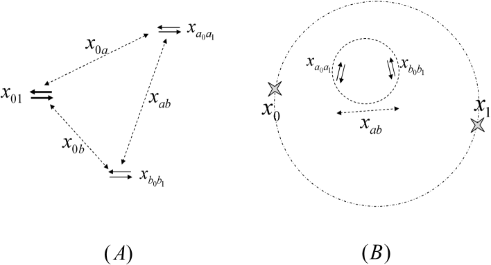
The factor $x_{ab}^{-2(\gamma_{a}+\gamma_{b}-\gamma)}$ characterizes the correlation of dipoles in impact parameter space. To see the significance of this factor, consider scattering of two dipoles $x_{a_{0}a_{1}},x_{b_{0}b_{1}}$ on a target dipole $x_{01}$ at large impact parameter. The scattering amplitude is given by

$$T_{Y}(x_{01};x_{a_{0}a_{1}},x_{b_{0}b_{1}})=\int\frac{d^{2}x}{2\pi x^{2}}\frac{d^{2}x^{\prime}}{2\pi x^{\prime 2}}\int d^{2}bd^{2}b^{\prime}n^{(2)}_{Y}(x_{01},xb,x^{\prime}b^{\prime})$$

$$\qquad\qquad\qquad\qquad\qquad\times A(x_{a_{0}a_{1}}x,x_{a}-\frac{x_{0}+x_{1}}{2}-b)A(x_{b_{0}b_{1}}x^{\prime},x_{b}-\frac{x_{0}+x_{1}}{2}-b^{\prime})$$

$$\qquad\qquad\qquad\qquad\approx\frac{\pi^{2}\alpha_{s}^{4}x_{a_{0}a_{1}}^{2}x_{b_{0}b_{1}}^{2}}{16\gamma_{a}^{2}(1-\gamma_{a})^{2}\gamma_{b}^{2}(1-\gamma_{b})^{2}}n^{(2)}_{Y}(x_{01},x_{a_{0}a_{1}},x_{b_{0}b_{1}})$$

$$\qquad\qquad\qquad\qquad\sim T_{Y}(x_{01},x_{a_{0}a_{1}},x_{0a})T_{Y}(x_{01},x_{b_{0}b_{1}},x_{0b})\left(\frac{x_{0a}x_{0b}}{x_{01}x_{ab}}\right)^{2(\gamma_{a}+\gamma_{b}-\gamma)}.$$ (3.18)

In the second line, we have used the same approximation as in Eq. (2.18). The last line should be taken with care since $\gamma_{a}$ as determined from Eq. (3.14) does not coincide with the anomalous dimension of $T(x_{01},x_{a_{0}a_{1}},x_{0a})$, the latter being determined from $\chi^{\prime}(\gamma_{a})Y=\ln\frac{x_{0a}^{4}}{x_{a_{0}a_{1}}^{2}x_{01}^{2}}$ (c.f., Eqs. (3.14), (3.16) and note that $\gamma\neq\gamma_{a}$). Even if we neglect this difference, we see from Eq. (3.18) that the factorization of two–dipole amplitude is explicitly violated by a nontrivial position–dependent factor.

$$\left(\frac{x_{0a}x_{0b}}{x_{01}x_{ab}}\right)^{2(\gamma_{a}+\gamma_{b}-\gamma)}\gg 1.$$ (3.19)

4 Improved calculation

Let us return to the integral appearing in Eq. (3.1).

$$I=\int d^{2}x_{\alpha}d^{2}x_{\beta}d^{2}x_{\gamma}E^{h,\bar{h}}(x_{0\gamma},x_{1\gamma})E^{h_{a},\bar{h}_{a}}(x_{a_{0}\alpha},x_{a_{1}\alpha})E^{h_{b},\bar{h}_{b}}(x_{b_{0}\beta},x_{b_{1}\beta})$$

$$\times\int\frac{d^{2}x_{2}d^{2}x_{3}d^{2}x_{4}}{x_{23}^{2}x_{34}^{2}x_{42}^{2}}E^{h,\bar{h}*}(x_{2\gamma},x_{3\gamma})E^{h_{a},\bar{h}_{a}*}(x_{2\alpha},x_{4\alpha})E^{h_{b},\bar{h}_{b}*}(x_{3\beta},x_{4\beta}).$$ (4.1)

Instead of first integrating over $x_{2,3,4}$ (‘reggeon coordinates’) as we did before, now we integrate over $x_{\alpha,\beta,\gamma}$ (‘Pomeron coordinates’, see, Fig. 2) first.

$$I=\frac{1}{(2\pi^{2})^{3}}\int\frac{d^{2}x_{2}d^{2}x_{3}d^{2}x_{4}}{x_{23}^{2}x_{34}^{2}x_{42}^{2}}\Bigl{(}b^{*}_{0,\nu}|\rho|^{2\gamma}F(\gamma,\gamma,2\gamma;\rho)F(\gamma,\gamma,2\gamma;\bar{\rho})+c.c.\Bigr{)}$$

$$\times\Bigl{(}b^{*}_{0,\nu_{a}}|\rho_{a}|^{2\gamma_{a}}F(\gamma_{a},\gamma_{a},2\gamma_{a};\rho_{a})F(\gamma_{a},\gamma_{a},2\gamma_{a};\bar{\rho}_{a})+c.c.\Bigr{)}$$

$$\times\Bigl{(}b^{*}_{0,\nu_{b}}|\rho_{b}|^{2\gamma_{b}}F(\gamma_{b},\gamma_{b},2\gamma_{b};\rho_{b})F(\gamma_{b},\gamma_{b},2\gamma_{b};\bar{\rho}_{b})+c.c.\Bigr{)},$$ (4.2)

where

$$\rho\equiv\frac{z_{01}z_{23}}{z_{02}z_{13}},\ \ \rho_{a}\equiv\frac{z_{a_{0}a_{1}}z_{24}}{z_{a_{0}2}z_{a_{1}4}},\ \ \rho_{b}\equiv\frac{z_{b_{0}b_{1}}z_{34}}{z_{b_{0}3}z_{b_{1}4}},$$ (4.3)

are anharmonic ratios. By assumption, $\rho_{a}$ and $\rho_{b}$ are small, and one may approximate $F(...;\rho_{a,b})\approx 1$. A remarkable point is that $\rho$ is small both in the limits of $x_{01}\to\infty$ and $x_{01}\to 0$ and one may approximate $F(...;\rho)\approx 1.$ Expanding the brackets, we get eight terms. The first term reads

$$I_{1}=\frac{1}{8\pi^{6}}b^{*}_{0,\nu}b^{*}_{0,\nu_{a}}b^{*}_{0,\nu_{b}}\int\frac{d^{2}x_{2}d^{2}x_{3}d^{2}x_{4}}{x_{23}^{2}x_{34}^{2}x_{42}^{2}}\left(\frac{x_{01}x_{23}}{x_{02}x_{13}}\right)^{2\gamma}\left(\frac{x_{a_{0}a_{1}}x_{24}}{x_{a2}x_{a4}}\right)^{2\gamma_{a}}\left(\frac{x_{b_{0}b_{1}}x_{34}}{x_{b3}x_{b4}}\right)^{2\gamma_{b}}$$ (4.4)

If we take the limit $x_{01}\to 0$, this is the same integral which gives the triple Pomeron vertex $f(\gamma,\gamma_{a},\gamma_{b})$.

$$\int\frac{d^{2}x_{2}d^{2}x_{3}d^{2}x_{4}}{x_{23}^{2}x_{34}^{2}x_{42}^{2}}\left(\frac{x_{01}x_{23}}{x_{02}x_{13}}\right)^{2\gamma}\left(\frac{x_{a_{0}a_{1}}x_{24}}{x_{a2}x_{a4}}\right)^{2\gamma_{a}}\left(\frac{x_{b_{0}b_{1}}x_{34}}{x_{b3}x_{b4}}\right)^{2\gamma_{b}}$$

$$\approx x_{01}^{2\gamma}x_{a_{0}a_{1}}^{2\gamma_{a}}x_{b_{0}b_{1}}^{2\gamma_{b}}\int\frac{d^{2}x_{2}d^{2}x_{3}d^{2}x_{4}}{x_{23}^{2}x_{34}^{2}x_{42}^{2}}\left(\frac{x_{23}}{x_{02}x_{03}}\right)^{2\gamma}\left(\frac{x_{24}}{x_{a2}x_{a4}}\right)^{2\gamma_{a}}\left(\frac{x_{34}}{x_{b3}x_{b4}}\right)^{2\gamma_{b}}$$

$$=x_{01}^{2\gamma}x_{a_{0}a_{1}}^{2\gamma_{a}}x_{b_{0}b_{1}}^{2\gamma_{b}}\frac{f(\gamma,\gamma_{a},\gamma_{b})}{x_{0a}^{2(\gamma+\gamma_{a}-\gamma_{b})}x_{0b}^{2(\gamma+\gamma_{b}-\gamma_{a})}x_{ab}^{2(\gamma_{a}+\gamma_{b}-\gamma)}}.$$ (4.5)

For a later use, we note that when $\gamma_{a}=\gamma_{b}$,

$$I_{1}=\frac{1}{8\pi^{6}}b^{*}_{0,\nu}b^{*2}_{0,\nu_{a}}f(\gamma,\gamma_{a},\gamma_{a})\left(\frac{x_{a_{0}a_{1}}x_{b_{0}b_{1}}}{x_{ab}^{2}}\right)^{2\gamma_{a}}\left(\frac{x_{01}x_{ab}}{x_{0a}x_{0b}}\right)^{2\gamma},\quad(x_{01}\to 0).$$ (4.6)

Eq. (4.5) should coincide with our previous result Eq. (3), so we obtain an identity

$$g(\gamma,\gamma_{a},\gamma_{b})f(\bar{\gamma},\bar{\gamma}_{a},\bar{\gamma}_{b})=\frac{1}{8\pi^{6}}b^{*}_{0,\nu}b^{*}_{0,\nu_{a}}b^{*}_{0,\nu_{b}}f(\gamma,\gamma_{a},\gamma_{b}).$$ (4.7)

Eq. (4.7) is a straightforward generalization of the relation between $f(\gamma,\gamma_{a},\gamma_{b})$ and $f(\bar{\gamma},\gamma_{a},\gamma_{b})$ derived in [32]. We also see that the previous approximation Eq. (3.6) misses the seven other terms in Eq. (4.2) which contribute equally to $n^{(2)}$ due to the symmetry $\gamma\leftrightarrow 1-\gamma$ of the integrals $\int d\gamma d\gamma_{a}d\gamma_{b}$. We take this into account by multiplying Eq. (4.4) by 8.

$$I\to\frac{1}{\pi^{6}}b^{*}_{0,\nu}b^{*}_{0,\nu_{a}}b^{*}_{0,\nu_{b}}\int\frac{d^{2}x_{2}d^{2}x_{3}d^{2}x_{4}}{x_{23}^{2}x_{34}^{2}x_{42}^{2}}\left(\frac{x_{01}x_{23}}{x_{02}x_{13}}\right)^{2\gamma}\left(\frac{x_{a_{0}a_{1}}x_{24}}{x_{a2}x_{a4}}\right)^{2\gamma_{a}}\left(\frac{x_{b_{0}b_{1}}x_{34}}{x_{b3}x_{b4}}\right)^{2\gamma_{b}}$$ (4.8)

Now we would like to evaluate this for $x_{01}\to\infty$. In the following, we assume that $\gamma_{a}=\gamma_{b}$, which will be approximately valid at the saddle point when $x_{a_{0}a_{1}}\sim x_{b_{0}b_{1}}$. Then Eq. (4.8) takes the form

$$I=\frac{1}{\pi^{6}}b^{*}_{0,\nu}b^{*2}_{0,\nu_{a}}\left(\frac{x_{a_{0}a_{1}}x_{b_{0}b_{1}}}{x^{2}_{ab}}\right)^{2\gamma_{a}}\int\frac{d^{2}x_{2}d^{2}x_{3}d^{2}x_{4}}{x_{23}^{2}x_{34}^{2}x_{42}^{2}}\left(\frac{x_{01}x_{23}}{x_{02}x_{13}}\right)^{2\gamma}\left(\frac{x_{24}x_{34}x_{ab}^{2}}{x_{a2}x_{a4}x_{b3}x_{b4}}\right)^{2\gamma_{a}}.$$ (4.9)

It is easy to see from the SL(2,C) invariance that the result of the integration must have the structure [In fact, this property holds only for $\gamma_{a}=\gamma_{b}$.]

$$I=\frac{1}{\pi^{6}}b^{*}_{0,\nu}b^{*2}_{0,\nu_{a}}\left(\frac{x_{a_{0}a_{1}}x_{b_{0}b_{1}}}{x^{2}_{ab}}\right)^{2\gamma_{a}}h\left(\rho^{\prime},\bar{\rho}^{\prime}\right),$$ (4.10)

where

$$\rho^{\prime}=\frac{z_{01}z_{ab}}{z_{0a}z_{1b}},$$ (4.11)

is the anharmonic ratio of the external points. In the limit $x_{01}\to 0$, $\rho^{\prime}\to 0$ and $h$ should reproduce Eq. (4.6).

$$h(\rho^{\prime},\bar{\rho}^{\prime})\approx f(\gamma,\gamma_{a},\gamma_{a})|\rho^{\prime}|^{2\gamma},\qquad(\rho^{\prime}\to 0).$$ (4.12)

Our observation is that the limit $x_{01}\to\infty$ also leads to $\rho^{\prime}\to 0$. Therefore, when $x_{01}\to\infty$,

$$I\approx\frac{1}{\pi^{6}}b^{*}_{0,\nu}b^{*2}_{0,\nu_{a}}f(\gamma,\gamma_{a},\gamma_{a})\left(\frac{x_{a_{0}a_{1}}x_{b_{0}b_{1}}}{x^{2}_{ab}}\right)^{2\gamma_{a}}\left(\frac{x_{01}x_{ab}}{x_{0a}x_{1b}}\right)^{2\gamma}$$

$$=8g(\gamma,\gamma_{a},\gamma_{a})f(\bar{\gamma},\bar{\gamma}_{a},\bar{\gamma}_{a})\left(\frac{x_{a_{0}a_{1}}x_{b_{0}b_{1}}}{x^{2}_{ab}}\right)^{2\gamma_{a}}\left(\frac{x_{01}x_{ab}}{x_{0a}x_{1b}}\right)^{2\gamma},$$ (4.13)

and we obtain the behavior of $n^{(2)}$ at the saddle point

$$n^{(2)}_{Y}(x_{0}x_{1};x_{a_{0}}x_{a_{1}},x_{b_{0}}x_{b_{1}})\sim\frac{1}{x^{2}_{a_{0}a_{1}}x_{b_{0}b_{1}}^{2}}e^{2\chi(\gamma_{a})Y}b^{*}_{0,\nu}b^{*2}_{0,\nu_{a}}f(\gamma,\gamma_{a},\gamma_{a})\left(\frac{x_{a_{0}a_{1}}x_{b_{0}b_{1}}}{x^{2}_{ab}}\right)^{2\gamma_{a}}\left(\frac{x_{01}x_{ab}}{x_{0a}x_{1b}}\right)^{2\gamma},$$ (4.14)

with $\gamma$ and $\gamma_{a}$ (and also $y$) determined from the saddle point equations

$$\chi(\gamma)=2\chi(\gamma_{a}),$$ (4.15)

$$\chi^{\prime}(\gamma)y=\ln\frac{x_{0a}^{2}x_{1b}^{2}}{x_{01}^{2}x_{ab}^{2}}\gg 1,$$ (4.16)

$$\chi^{\prime}(\gamma_{a})(Y-y)=\ln\frac{x_{ab}^{2}}{x_{a_{0}a_{1}}^{2}}\gg 1.$$ (4.17)

Note that $\frac{1}{2}<\gamma_{a}<\gamma<1$.

Eq. (4.14) is valid both for $x_{01}\ll x_{ab}$ and $x_{01}\gg x_{ab}$. Due to conformal symmetry, the two cases of Fig. 3 are mathematically identical. In the latter case, if the dipole $x_{ab}$ is deeply inside the parent dipole $x_{01}$, one can make an approximation

$$\left(\frac{x_{01}x_{ab}}{x_{0a}x_{1b}}\right)^{2\gamma}\approx\left(\frac{x_{ab}}{x_{01}}\right)^{2\gamma}.$$ (4.18)

It is interesting to note that in the same limit we may rewrite $n^{(2)}$ as

$$n^{(2)}_{Y}\approx\frac{f(\gamma,\gamma_{a},\gamma_{a})}{x_{a_{0}a_{1}}^{2}x_{b_{0}b_{1}}^{2}}\int^{Y}_{0}dy\frac{x_{ab}^{2}}{x_{01}^{2}}n_{y}(x_{01},x_{ab})\frac{x_{a_{0}a_{1}}^{2}}{x_{ab}^{2}}n_{Y-y}(x_{ab},x_{a_{0}a_{1}})\frac{x_{b_{0}b_{1}}^{2}}{x_{ab}^{2}}n_{Y-y}(x_{ab},x_{b_{0}b_{1}}).$$ (4.19)

Eq. (4.19) provides an intuitive understanding of the result. The parent dipole $x_{01}$ emits a child dipole $x_{ab}$ inside the area $x_{01}^{2}$ with uniform probability (c.f., Eq. (2.15)). The geometrical factor $x_{ab}^{2}/x_{01}^{2}$ specifies the location of the dipole $x_{ab}$. Then the dipole $x_{ab}$ splits into two dipoles of similar size $\sim x_{ab}$ through the triple Pomeron vertex, $f(\gamma,\gamma_{a},\gamma_{a})$. Finally, each of the two dipoles emits a child dipole of size $x_{a_{0}a_{1}}$ (or $x_{b_{0}b_{1}}$) inside the area $\sim x_{ab}^{2}$ again with uniform probability, and the two child dipoles $x_{a_{0}a_{1}}$ and $x_{b_{0}b_{1}}$ roughly fall within a distance $x_{ab}$ (see, Fig. 3B). Another representation of $n^{(2)}$ is (c.f., Eq. (2.5))

$$n^{(2)}_{Y}\propto\int^{Y}_{0}dyT_{y}(x_{01},x_{ab})T_{Y-y}(x_{ab},x_{a_{0}a_{1}})T_{Y-y}(x_{ab},x_{b_{0}b_{1}}),$$ (4.20)

which may be a useful form to include effects beyond the BFKL evolution.

Finally, we consider how the approach to saturation is modified in the presence of power–law correlations in the target. The scattering amplitude of two dipoles off a large onium of size $x_{01}$ at small impact parameter can be computed similarly as before

$$T_{Y}^{(2)}(x_{01};x_{a_{0}a_{1}},x_{b_{0}b_{1}})\sim\alpha_{s}^{4}x_{a_{0}a_{1}}^{2}x_{b_{0}b_{1}}^{2}n_{Y}(x_{01};x_{a_{0}a_{1}},x_{b_{0}b_{1}})$$

$$\qquad\qquad\qquad\qquad\sim T_{Y}(x_{01},x_{a_{0}a_{1}},b\approx 0)T_{Y}(x_{01},x_{b_{0}b_{1}},b\approx 0)\left(\frac{x_{01}}{x_{ab}}\right)^{2(2\gamma_{a}-\gamma)}.$$ (4.21)

The power law correlation Eq. (4.21) is remarkable in view of the fact that the single dipole distribution has essentially no $b$–dependence deep inside the dipole $x_{01}$. Due to the enhancement factor, $\left(\frac{x_{01}}{x_{ab}}\right)^{2(2\gamma_{a}-\gamma)}\gg 1$, the problem of unitarity for $T^{(2)}$ is severer than that for $T$. The condition $T^{(2)}\leq 1$ is roughly equivalent to requiring that the exponential factor of $n^{(2)}$ vanishes along the saturation line $x_{a_{0}a_{1}}=x_{b_{0}b_{1}}=1/Q_{pairsat}$

$$2\chi(\gamma_{a})Y-\gamma\ln\frac{x_{01}^{2}}{x_{ab}^{2}}-2\gamma_{a}\ln(x_{ab}^{2}Q_{pairsat}^{2})=0.$$ (4.22)

Solving this equation with the conditions Eqs. (4.15)-(4.17), one finds that

$$Q^{2}_{pairsat}=\frac{1}{x_{01}^{2}}e^{\frac{\chi(\gamma_{a})}{\gamma_{a}}Y}\left(\frac{x_{01}^{2}}{x_{ab}^{2}}\right)^{1-\frac{\gamma}{2\gamma_{a}}}=\frac{1}{x_{ab}^{2}}\exp\left(\frac{\chi^{\prime}(\gamma)-\frac{\chi(\gamma)}{\gamma}}{\frac{\chi^{\prime}(\gamma)}{\chi^{\prime}(\gamma_{a})}-\frac{2\gamma_{a}}{\gamma}}Y\right).$$ (4.23)

Since $\gamma$ and $\gamma_{a}$ depend on coordinates, there is not a unique way of writing $Q_{pairsat}$. The first expression shows that, when $\gamma_{a}\approx\gamma_{s}$, the onset of unitarity corrections is much earlier than the single dipole scattering case, $Q_{pairsat}\gg Q_{s}$ (c.f., Eq. (2.22)). This is quite a contrast to the result $Q_{s}\approx Q_{pairsat}$ which would follow from the assumption of factorization $T^{(2)}\approx T^{2}$. The second expression of Eq. (4.23) emphasizes that $Q_{pairsat}$ is not an intrinsic quantity of the target, but depends rather sensitively on the configuration of the projectile.

References

• [1] E. A. Kuraev, L. N. Lipatov and V. S. Fadin, Sov. Phys. JETP 45 (1977) 199; I. I. Balitsky and L. N. Lipatov, Sov. J. Nucl. Phys.  28 (1978) 822.
• [2] G. P. Salam, Nucl. Phys. B 449 (1995) 589; Nucl. Phys. B 461 (1996) 512; A. H. Mueller and G. P. Salam, Nucl. Phys. B 475 (1996) 293.
• [3] E. Iancu and A. H. Mueller, Nucl. Phys. A 730 (2004) 494; M. Kozlov and E. Levin, Nucl. Phys. A 739 (2004) 291.
• [4] E. Iancu, A. H. Mueller and S. Munier, Phys. Lett. B 606 (2005) 342.
• [5] A. H. Mueller and A. I. Shoshi, Nucl. Phys. B 692 (2004) 175.
• [6] E. Iancu and D.N. Triantafyllopoulos, Nucl. Phys. A 756 (2005) 419; Phys. Lett. B 610 (2005) 253; A. H. Mueller, A. I. Shoshi and S. M. H. Wong, Nucl. Phys. B 715 (2005) 440; A. Kovner and M. Lublinsky, Phys. Rev. D71 (2005) 085004.
• [7] G. Soyez, Phys. Rev. D 72 (2005) 016007; R. Enberg, K. Golec-Biernat and S. Munier, Phys. Rev. D 72 (2005) 074021; N. Armesto and J. G. Milhano, Phys. Rev. D 73 (2006) 114003.
• [8] Y. Hatta, E. Iancu, C. Marquet, G. Soyez and D. N. Triantafyllopoulos, Nucl. Phys. A 773 (2006) 95; E. Iancu, C. Marquet and G. Soyez, Nucl. Phys. A 780 (2006) 52; M. Kozlov, A. I. Shoshi and B. W. Xiao, arXiv:hep-ph/0612053.
• [9] E. Iancu and L. McLerran, arXiv:hep-ph/0701276.
• [10] L. V. Gribov, E. M. Levin and M. G. Ryskin, Phys. Rept.  100 (1983) 1.
• [11] A. H. Mueller and J. w. Qiu, Nucl. Phys. B 268 (1986) 427.
• [12] L. McLerran and R. Venugopalan, Phys. Rev. D49 (1994) 2233.
• [13] I. Balitsky, Nucl. Phys. B463 (1996) 99; Y. V. Kovchegov, Phys. Rev. D 60 (1999) 034008; J. Jalilian-Marian, A. Kovner, A. Leonidov and H. Weigert, Phys. Rev. D59 (1999) 014014; J. Jalilian-Marian, A. Kovner and H. Weigert, Phys. Rev. D59 (1999) 014015; E. Iancu, A. Leonidov and L. McLerran, Nucl. Phys. A692 (2001) 583; E. Ferreiro, E. Iancu, A. Leonidov and L. McLerran, Nucl. Phys. A703 (2002) 489.
• [14] A. H. Mueller, Nucl. Phys. B 415 (1994) 373.
• [15] A. H. Mueller and B. Patel, Nucl. Phys. B 425 (1994) 471.
• [16] A. H. Mueller, Nucl. Phys. B 437 (1995) 107.
• [17] E. Avsar, G. Gustafson and L. Lonnblad, arXiv:hep-ph/0610157.
• [18] R. Peschanski, Phys. Lett. B 409 (1997) 491.
• [19] A. Bialas and R. Peschanski, Phys. Lett.  B 355 (1995) 301.
• [20] M. Braun and D. Treleani, Eur. Phys. J.  C 18 (2001) 511.
• [21] L. N. Lipatov, Sov. Phys. JETP 63 (1986) 904.
• [22] L. N. Lipatov, Phys. Rept.  286 (1997) 131.
• [23] H. Navelet and R. Peschanski, Nucl. Phys. B 507 (1997) 353.
• [24] H. Navelet and S. Wallon, Nucl. Phys. B 522 (1998) 237.
• [25] E. Iancu, K. Itakura and L. McLerran, Nucl. Phys. A 708 (2002) 327.
• [26] A. H. Mueller and D. N. Triantafyllopoulos, Nucl. Phys. B 640 (2002) 331.
• [27] S. Munier and R. Peschanski, Phys. Rev. Lett.  91 (2003) 232001.
• [28] S. Munier and S. Wallon, Eur. Phys. J. C 30 (2003) 359; C. Marquet, R. Peschanski and G. Soyez, Nucl. Phys. A 756 (2005) 399.
• [29] M. A. Braun and G. P. Vacca, Eur. Phys. J. C 6 (1999) 147.
• [30] J. Bartels and M. Wusthoff, Z. Phys. C 66 (1995) 157; J. Bartels, L. N. Lipatov and M. Wusthoff, Nucl. Phys. B 464 (1996) 298.
• [31] A. Bialas, H. Navelet and R. Peschanski, Phys. Rev. D 57 (1998) 6585.
• [32] G. P. Korchemsky, Nucl. Phys. B 550 (1999) 397.