On The Equivalence of Soft and Zero-Bin Subtractions

Abstract

Zero-bin subtractions are required to avoid double counting soft contributions in collinear loop integrals in Soft-Collinear Effective Theory (SCET). In traditional approaches to factorization, double counting is avoided by dividing jet functions by matrix elements of soft Wilson lines. In this paper, we compare the two approaches to double counting, studying the quark form factor and deep inelastic scattering (DIS) as $x_{B}\to 1$ as examples. We explain how the zero-bin subtractions in SCET are required to reproduce the well-established factorization theorem for DIS as $x_{B}\to 1$. We study one-loop virtual contributions to the quark form factor and real gluon emission diagrams in DIS. The two approaches to double counting are equivalent if dimensional regularization (DR) is used to regulate infrared (IR) divergences. We discuss in detail ambiguities in the calculation of one-loop scaleless integrals in DR in SCET and perturbative QCD. We also demonstrate a nontrivial check of the equivalence of the zero-bin subtraction and the soft Wilson line subtraction in the virtual two-loop Abelian contributions to the quark form factor.

I Introduction

High-energy processes with hadrons in either the initial or final state are amenable to perturbative QCD (pQCD) treatment as long as there is a hard scale, $Q$, much larger than $\Lambda_{\rm QCD}$. The essential idea of pQCD factorization Collins:1989gx is to separate the different relevant scales into a well-defined quantities that capture the physics at the given scale. By doing so one is then able to distinguish the perturbative short-distance contribution from the nonperturbative long-distance one.

In order to properly establish such factorization of scales it is clear that one has to avoid double counting among the functions that appear in the factorized physical quantity. In general these nonperturbative functions receive leading contributions (in powers of $\Lambda_{\rm QCD}^{2}/Q^{2}$) from specific regions in momentum space. For example, the contribution to a jet function may be dominated by partons with momenta whose components scale as

$$(p^{+},p^{-},p^{\perp})\sim Q(1,\lambda^{2},\lambda)\,,$$ (1)

where $\lambda$ characterizes the off-shellness of the partons in the jet function, and $\lambda^{2}\sim Q\Lambda_{\rm QCD}$ or $\Lambda_{\rm QCD}^{2}$, depending on the process considered. In principle, one could restrict all momenta appearing in loop calculations to satisfy the scaling in Eq. (1), but this is impractical. Instead one typically integrates over all momentum space in loop integrations, making approximations appropriate for the assumed scaling. This practice is well-known in, for example, the method of regions Beneke:1997zp , where approximations appropriate to a specific momentum region are performed at the level of the integrand, but the integrals are over all momentum space. In cases where contributions from other momentum regions are not sub-leading, one encounters double counting.

Consider, for example, deep inelastic scattering (DIS) in the end point region, $x_{B}\rightarrow 1$, where $x_{B}$ is the well-known Bjorken variable. In this region, Sterman Sterman:1986aj has shown that to all orders in perturbation theory one can (re-)factorize the non-singlet DIS structure function in moment space according to the formulae

$$F_{2,N}(Q^{2})=H\times\phi_{N}\times S_{N}\times J_{N}\,,$$ (2)

Here $F_{2,N}(Q^{2})$ is the $N$th moment of the structure function and $x_{B}\to 1$ implies $N\gg 1$. $H$ is the hard contribution, $\phi_{N}$ is the $N$th moment of a modified parton distribution function (PDF), $J_{N}$ is the $N$th moment of an outgoing jet function, and $S_{N}$ is the $N$th moment of a soft factor representing the emission of soft gluons. Explicit and gauge invariant expressions for the PDF, jet, and soft functions will be given below. In the factorization theorem of Ref. Sterman:1986aj , the jet, soft, and parton distribution functions are not defined in a gauge invariant way, and through a judicious choice of gauge one can eliminate double counting. However when one defines the same quantities using Wilson lines to make them gauge invariant, the factorization theorem breaks down and has to be modified to take into account the double counting of soft momentum modes in the soft factor, $S_{N}$, and in the collinear matrix elements, $J_{N}$ and $\phi_{N}$. The Wilson lines in the matrix elements are the cause of the double counting problems. In Ref. Akhoury:1998gs , it was proposed that for gauge invariant quantities the factorization theorem should take the form

$$F_{2,N}(Q^{2})=H\left(\frac{\phi_{N}}{S_{N}}\right)S_{N}\left(\frac{J_{N}}{S_{N}}\right)\,.$$ (3)

A similar factorization theorem with a soft factor subtracted from the transverse momentum dependent PDF and jet function was also proposed by Ji, et. al. Ji:2004wu for semi-inclusive DIS. Ref. Ji:2004wu checked the theorem explicitly at one-loop and gave arguments for the theorem to hold to all orders in perturbation theory. Another well studied quantity in pQCD is the quark form factor and its factorization into jets and soft contributions. The double counting problem for this quantity is studied in Refs. Collins:1989bt ; Collins:1999dz , where it is argued that the same soft factor has to be subtracted from each one of the two collinear jets, in a manner similar to Eq. (3), to avoid double counting.

Recently, the problem of factorization has been addressed in an effective field theory approach using Soft Collinear Effective Theory (SCET) Bauer:2000yr ; Bauer:2001yt . In this approach to factorization, QCD is matched onto SCET, a theory containing collinear and soft modes whose momenta scale as

$${\rm collinear} \sim Q(1,\lambda^{2},\lambda)$$

$${\rm soft} \sim Q(\lambda^{2},\lambda^{2},\lambda^{2})\,.$$ (4)

After matching QCD onto SCET, a field redefinition Bauer:2001yt can be used to decouple the soft and collinear modes at the level of the Lagrangian. In SCET, jet functions are matrix elements of collinear fields and soft functions are matrix elements of soft fields. Note that in this paper the terms soft and collinear are defined by Eq. (I). For example, if a gluon whose momentum components all scale as $O(Q\lambda^{2})$ is emitted from a jet with small angle we still refer to it as a soft gluon.

The subject of double counting has gained renewed interest in the context of SCET due to the work of Manohar and Stewart Manohar:2006nz . In SCET, power counting is made manifest using the label formalism Georgi:1990um . Let $\phi(x)$ denote a generic full theory field, the corresponding collinear field in SCET, $\phi_{\hat{p}}(x)$, is defined by

$$\phi(x)=\sum_{\hat{p}\neq 0}e^{-i\hat{p}\cdot x}\phi_{\hat{p}}(x)\,.$$ (5)

The $\hat{p}$ are $O(Q,Q\lambda)$ label momenta which correspond to the large parts of the collinear momenta, while derivatives on $\phi_{\hat{p}}(x)$ give the $O(Q\lambda^{2})$ residual momenta. Loop integrations involve both a sum over labels and an integral over the residual momentum which in practical calculations are combined into an integral over all momentum space,

$$\sum_{\tilde{p}}\int d^{d}k\longrightarrow\int d^{d}l\,.$$ (6)

But this raises the issue of double counting, as the integral over all momentum space includes the region in which the label momentum vanishes - the “zero-bin” - which is already included in the soft sector of the theory. To correctly calculate the collinear graphs, one must subtract the zero-bin contributions. The zero-bin subtraction is necessary for the proper interpretation of $1/\epsilon$ poles in SCET loops Manohar:2006nz , and also necessary so that collinear plus soft real gluon emission graphs correctly reproduce real gluon emission QCD diagrams in the appropriate regions of phase space Manohar:2006nz ; Fleming:2006cd .

The zero-bin subtraction in SCET is clearly related to the soft subtraction in Eq. (3). In calculating the zero-bin contribution to a particular Feynman graph, one must apply SCET power counting. In the minimal zero-bin subtraction scheme of Ref. Manohar:2006nz the zero-bin contribution is only removed if its contribution scales as $\lambda^{0}$, i.e., is leading order in SCET power counting. Only the zero-bin of the $O(Q\lambda^{2})$ component of the gluon couples to collinear fields at $O(\lambda^{0})$ so in this scheme collinear couplings to other zero-bin modes can be neglected. Exploiting this fact, Ref. Lee:2006nr shows that the difference between calculating collinear matrix elements naively and including the zero-bin subtraction amounts to using two different collinear Lagrangians that are related by a field redefinition of the collinear fields Lee:2006nr . This field redefinition is similar to the field redefinition that is used to decouple soft modes from collinear modes to prove factorization in SCET. The field redefinition can be used to decouple the zero-bin mode from collinear modes at the price of inserting zero-bin Wilson lines into the collinear matrix elements. Thus, the naively evaluated collinear matrix element factorizes into a properly evaluated collinear matrix and a matrix element of zero-bin Wilson lines, establishing the equivalence of zero-bin subtractions and soft Wilson line subtractions at lowest order in $\lambda$. At higher orders in $\lambda$, zero-bin modes of other components of the gluon field are important so it seems that the equivalence only holds to lowest order in $\lambda$.

The purpose of this paper is to study the equivalence between zero-bin subtractions and the soft Wilson line subtractions in more detail. We focus on the on-shell quark form factor and the factorization theorem for DIS as $x_{B}\to 1$. One important issue is the choice of IR regulator in the calculation of the zero-bin contribution. The field redefinition which decouples the soft or zero-bin modes and collinear modes will only leave on-shell matrix elements invariant, and therefore off-shellness is not a suitable regulator Bauer:2003td . Soft Wilson line subtractions and zero-bin subtractions are not equivalent if offshellness is used to regulate the IR divergences.

In our calculation of the quark form factor, we will use DR to regulate both ultraviolet (UV) and IR divergences. The individual one-loop soft diagrams, the collinear diagrams and their zero-bin subtractions are all ill-defined, and only their sum yields a well-defined result which reproduces the IR divergences of QCD. Fortunately, in this case the equivalence of the soft and the zero-bin subtractions can be easily established at the level of the integrands. At higher orders the zero-bin subtraction involves an iterative procedure which requires the subtraction of graphs in which some lines have collinear momentum and some have soft momentum, so demonstrating the equivalence of soft and zero-bin subtractions at higher orders is somewhat subtle. For example, one has to be careful about the order in which limits are taken to correctly compute the zero-bin subtraction at two loops. Another issue is that the equivalence of zero-bin and soft subtractions does not hold at the level of individual Feynman diagrams, but only for the sum of all diagrams at a given order. In some cases this requires a cancellation between the zero-bins that appear in different diagrams. In this paper, we explore these issues by calculating the zero-bin subtractions in the two-loop abelian diagrams contributing to the quark form factor. We also show that they are equivalent to soft subtraction.

Another important point of this paper is to emphasize the importance of the zero-bin subtractions in the collinear matrix elements that appear in the SCET derivation of the endpoint factorization in DIS as $x_{B}\to 1$. We will assume a factorization theorem of the form of Eq. (2) where the definitions of $S_{N}$, $\phi_{N}$, and $J_{N}$ in terms of SCET fields will be given below. We will show that the one-loop zero-bin contributions to $\phi_{N}$ and $J_{N}$ are equal to $S_{N}$, which confirms Eq. (3). We will also show that at one-loop Eq. (3) reproduces the large $N$ limit of the full QCD calculation of DIS as $x_{B}\to 1$. In these calculations we again use DR to regulate the IR divergences. Our results are consistent with those in Ref. Chen:2006vd , however, in our treatment all Wilson lines are defined on the light-cone. For other SCET treatments of DIS in the $x_{B}\to 1$ limit, see Refs. Manohar:2003vb ; Becher:2006mr ; Chay:2005rz .

This paper is organized as follows. In section II, we discuss the space-like quark form factor in SCET and present one-loop results for the various contributions. Once zero-bin contributions are included it is straightforward to verify that SCET reproduces the IR divergences of QCD. In section III, we give our analysis of DIS at $x\to 1$ in SCET. In section IV, we study the zero-bin subtractions for two-loop virtual abelian contributions to the quark form factor and demonstrate agreement with the soft Wilson line subtractions. In section V we conclude.

II Zero-Bin at One-Loop: Quark Form Factor

In this section we calculate the quark form factor to one loop using DR to regulate both the UV and IR. It is straightforward to see that the zero-bin subtractions are reproduced by the soft subtractions for this choice of regulator. The quark form factor may be the simplest quantity to analyze in SCET, however it serves well to establish some of the relevant issues. We take the incoming quark to be moving along the $+z$ direction so its four-momentum is $p_{1}^{\mu}=(p_{1}^{+},p_{1}^{-},p_{1}^{\perp})=(\frac{Q}{\sqrt{2}},0,0)=\frac{Q}{\sqrt{2}}n^{\mu}$. The incoming quark scatters off a space-like photon whose invariant mass is $q^{2}\equiv-Q^{2}<0$. The final state quark is moving in the $-z$ direction so its momentum is $p_{2}^{\mu}=(p_{2}^{+},p_{2}^{-},p_{2}^{\perp})=(0,\frac{Q}{\sqrt{2}},0)=\frac{Q}{\sqrt{2}}{\bar{n}}^{\mu}$.

The full QCD electromagnetic current, $j^{\mu}={\bar{\psi}}(x)\gamma^{\mu}\psi(x)$, is matched onto an effective one,

$$j^{\mu} = C(Q^{2})j^{\mu}_{eff}=C(Q^{2})\ \bar{\xi}_{\bar{n}}W_{\bar{n}}\gamma^{\mu}W_{n}^{\dagger}\xi_{n}$$ (7)

$$= C(Q^{2})\ \bar{\xi}^{(0)}_{{\bar{n}}}W^{(0)}_{{\bar{n}}}Y^{\dagger}_{{\bar{n}}}\gamma^{\mu}Y_{n}W^{(0)\dagger}_{n}\xi^{(0)}_{n}\,.$$

The manipulations performed in Eq. (7) are standard in the SCET formalism. The form of the current is fixed by collinear gauge invariance. The second line is a consequence of making the field redefinition of the collinear quark and gluon fields that decouples soft gluons from the collinear sector of the leading order SCET lagrangian. The collinear Wilson line, $W_{n}$, and the soft Wilson line, $Y_{n}$, are given in momentum space by

$$W_{n}=\sum_{m=0}^{\infty}\sum_{{\rm perms}}\frac{(-g)^{m}}{m!}\frac{\bar{n}\cdot A_{n,q_{1}}\cdots\bar{n}\cdot A_{n,q_{m}}}{\bar{n}\cdot q_{1}\bar{n}\cdot(q_{1}+q_{2})\cdots\bar{n}\cdot(\sum_{i=1}^{m}q_{i})}\ ,$$ (8)

and

$$Y_{n}=\sum_{m=0}^{\infty}\sum_{{\rm perms}}\frac{(-g)^{m}}{m!}\frac{n\cdot A_{s}\cdots n\cdot A_{s}}{n\cdot q_{1}n\cdot(q_{1}+q_{2})\cdots n\cdot(\sum_{i=1}^{m}q_{i})}\ .$$ (9)

$A_{n,q_{i}}$ is a collinear gluon field and all $\bar{n}\cdot q_{i}$ scale as $Q$. $A_{s}$ stands for soft gluon field and $n\cdot q_{i}$ scales as $Q\lambda^{2}$.

The matrix element of $j_{eff}^{\mu}$ factorizes into

$$\langle q(p_{2})|j^{\mu}|q(p_{1})\rangle=C(Q^{2})\gamma^{\mu}[J_{out}\times\gamma^{\mu}\times J_{in}\times S]\,,$$ (10)

where the jet and soft functions are defined by

$$J_{in}=\langle 0|W^{(0)\dagger}_{n}\xi^{(0)}_{n}|q(p_{1})\rangle,\,\,\,\,J_{out}=\langle q(p_{2})|{\bar{\xi}^{(0)}}_{{\bar{n}}}W^{(0)}_{{\bar{n}}}|0\rangle,\,\,\,\,S=\langle 0|Y^{\dagger}_{\bar{n}}Y_{n}|0\rangle\,\,.$$ (11)

In the jet functions the fields are collinear so only fields with nonvanishing labels appear. As argued by Lee and Sterman Lee:2006nr , only the zero-bin of the $n\cdot A_{n,q}$ component of the collinear gluon couples to $\xi^{(0)}_{n}$ at leading order in $\lambda$. Furthermore, the Wilson line, $W_{n}^{(0)\dagger}$, which has no zero-bin gluon is related to one with a zero-bin by multiplication by a Wilson line constructed from the zero-bin component of the ${\bar{n}}\cdot A_{n,q}$ gluon. Thus the collinear matrix element is equal to the naively evaluated matrix element divided by a matrix element of soft Wilson lines:

$$\langle 0|W^{(0)\dagger}_{n}\xi^{(0)}_{n}|q(p_{1})\rangle=\frac{\langle 0|{\hat{W}}^{\dagger}_{n}{\hat{\xi}}_{n}|q(p_{1})\rangle}{\langle 0|Y^{\dagger}_{\bar{n}}Y_{n}|0\rangle}\,\,,$$ (12)

where

$$Y_{n}(x)=P\mathrm{exp}\left[ig_{s}\int_{-\infty}^{0}dsn\cdot A_{n,0}(ns+x)\right]\,\,,$$ (13)

$A_{n,0}$ is the zero-bin of the collinear gluon, and our definition of the covariant derivative is $D^{\mu}=\partial^{\mu}-ig_{s}A^{\mu}$. We will use the same notation for the soft Wilson line and the zero-bin Wilson line because the matrix elements are identical and it is always clear from context which is relevant. In Eq. (12) the hats on the fields signify that $\hat{W}_{n}^{\dagger}$ contains the zero-bin gluon and that the Lagrangian includes the coupling of $\hat{\xi}_{n}$ to zero-bin gluons, so this matrix element corresponds to the naive evaluation of the collinear matrix element. In our notation $\langle 0|W^{(0)\dagger}_{n}\xi^{(0)}_{n}|q(p_{1})\rangle$ corresponds to $\langle 0|W^{\prime\dagger}_{n}{\xi^{\prime}}_{n}|q(p_{1})\rangle$ of Ref. Lee:2006nr , $\langle 0|{\hat{W}}^{\dagger}_{n}{\hat{\xi}}_{n}|q(p_{1})\rangle$ corresponds to $\langle 0|W^{\prime\prime\dagger}_{n}\xi^{\prime\prime}_{n}|q(p_{1})\rangle$, $Y_{n}$ corresponds to $U_{n}^{\dagger}$, and $Y_{\bar{n}}$ corresponds to $\Omega_{n}$.

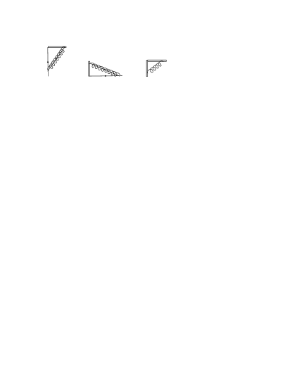
Figure 1: The quark form factor in SCET. In the first two graphs the thick line attached to the fermion line represents a collinear Wilson line, while in the last graph both thick lines are soft Wilson lines.

At one-loop the Feynman diagrams that contribute to the collinear $n$-jet, collinear $\bar{n}$-jet and the soft factor are given in Fig. 1. All these diagrams are scaleless in DR and therefore all integrals will vanish when one sets $\varepsilon_{\text{UV}}=\varepsilon_{\text{IR}}$. Using SCET Feynman rules to calculate the $n$-collinear diagram and naively integrating over all momentum space, the result is

$$I_{n}=-2ig_{s}^{2}C_{F}(\mu^{2})^{\varepsilon}\int\frac{d^{d}k}{(2\pi)^{d}}\frac{{\tilde{p}}-k^{+}}{[-2{\tilde{p}}k^{-}+k^{2}+i0][-k^{+}+i0][k^{2}+i0]}\ ,$$ (14)

where ${\tilde{p}}\equiv p_{1}^{+}=p_{2}^{-}=\frac{Q}{\sqrt{2}}$. Note that the collinear graph is not $I_{n}$ but rather $I_{n}-I_{n,0}$, where $I_{n,0}$ is the zero-bin contribution. We refer to $I_{n}$ as the naive $n$-collinear contribution. The naive ${\bar{n}}$-collinear contribution is similar,

$$I_{\bar{n}}=-2ig_{s}^{2}C_{F}(\mu^{2})^{\varepsilon}\int\frac{d^{d}k}{(2\pi)^{d}}\frac{{\tilde{p}}-k^{-}}{[-2{\tilde{p}}k^{+}+k^{2}+i0][-k^{-}+i0][k^{2}+i0]}\ ,$$ (15)

and the soft contribution is

$$I_{s}=-ig_{s}^{2}C_{F}(\mu^{2})^{\varepsilon}\int\frac{d^{d}k}{(2\pi)^{d}}\frac{1}{(-k^{+}+i0)(-k^{-}+i0)(k^{2}+i0)}\ .$$ (16)

Let us now compute the zero-bin subtraction for $I_{n}$. It is easy to check that the zero-bin associated with the virtual fermion line is subleading in $\lambda$. The only zero-bin needed is associated with the virtual gluon. In this zero-bin region, $k^{+}$ scales as $Q\lambda^{2}$ instead of $Q$ so the numerator is simply $\tilde{p}$. Furthermore, $k^{2}$ scales $Q^{2}\lambda^{4}$ instead of $Q^{2}\lambda^{2}$ thus it should be dropped relative to ${\tilde{p}}k^{-}$. Similar arguments hold for $I_{\bar{n}}$. The result is simply that

$$I_{n,0} = I_{\bar{n},0}=-ig_{s}^{2}C_{F}(\mu^{2})^{\varepsilon}\int\frac{d^{d}k}{(2\pi)^{d}}\frac{1}{(-k^{+}+i0)(-k^{-}+i0)(k^{2}+i0)}\,$$ (17)

$$= I_{s}$$

The complete one-loop SCET contribution to the quark form factor is

$$I = (I_{n}-I_{n,0})+(I_{\bar{n}}-I_{{\bar{n}},0})+I_{s}$$ (18)

$$= I_{n}+I_{\bar{n}}-I_{s}\,.$$

Note that the net effect of the zero-bin subtractions at one-loop is to reverse the sign of the soft contributions. Thus the zero-bin subtraction and soft subtraction of Eq. (3) yield the same results for the one-loop graphs when they are regulated in DR.

One subtlety in Eq. (18) is that the integrals $I_{n}$, $I_{\bar{n}}$ and $I_{s}$ are all ill-defined. However, in Eq. (18) the integrands can be rearranged so that $I$ is expressed in terms of integrals which are well-defined, then it is straightforward to show that $I$ reproduces the IR of QCD. Eq. (18) can be written as

$$I = -2ig_{s}^{2}C_{F}(\mu^{2})^{\varepsilon}\int\frac{d^{d}k}{(2\pi)^{d}}\left\{\frac{2{\tilde{p}}[{\tilde{p}}-k^{+}-k^{-}]}{[-2{\tilde{p}}k^{+}+k^{2}+i0][-2{\tilde{p}}k^{-}+k^{2}+i0][k^{2}+i0]}\right.$$ (19)

$$+\frac{2}{[-2{\tilde{p}}k^{+}+k^{2}+i0][-2{\tilde{p}}k^{-}+k^{2}+i0]}$$

$$\left.-\frac{k^{2}}{2[-2{\tilde{p}}k^{+}+k^{2}+i0][-2{\tilde{p}}k^{-}+k^{2}+i0][-k^{+}+i0][-k^{-}+i0]}\right\}$$

$$\equiv I_{1}+I_{2}+I_{3}\,\,,$$

where

$$I_{1} = -2ig_{s}^{2}C_{F}(\mu^{2})^{\varepsilon}\int\frac{d^{d}k}{(2\pi)^{d}}\frac{2{\tilde{p}}(\tilde{p}-k^{+}-k^{-})}{[-2{\tilde{p}}k^{+}+k^{2}+i0][-2{\tilde{p}}k^{-}+k^{2}+i0][k^{2}+i0]}$$ (20)

$$= -\frac{\alpha_{s}}{2\pi}C_{F}\left(\frac{4\pi\mu^{2}}{Q^{2}}\right)^{\varepsilon}\frac{\Gamma(1+\varepsilon_{\rm IR})\Gamma^{2}(-\varepsilon_{\rm IR})}{\Gamma(2-2\varepsilon_{\rm IR})}\,\,,$$

$$I_{2} = -2ig_{s}^{2}C_{F}(\mu^{2})^{\varepsilon}\int\frac{d^{d}k}{(2\pi)^{d}}\frac{2}{[-2{\tilde{p}}k^{+}+k^{2}+i0][-2{\tilde{p}}k^{-}+k^{2}+i0]}$$ (21)

$$=+\frac{\alpha_{s}}{2\pi}C_{F}\left(\frac{4\pi\mu^{2}}{Q^{2}}\right)^{\varepsilon}\frac{2\,\Gamma^{2}(1-\varepsilon_{\rm UV})\Gamma(\varepsilon_{\rm UV})}{\Gamma(2-2\varepsilon_{\rm UV})}\,\,,$$

$$I_{3} = -2ig_{s}^{2}C_{F}(\mu^{2})^{\varepsilon}\int\frac{d^{d}k}{(2\pi)^{d}}\frac{-k^{2}}{2[-2{\tilde{p}}k^{+}+k^{2}+i0][-2{\tilde{p}}k^{-}+k^{2}+i0][-k^{+}+i0][-k^{-}+i0]}$$ (22)

$$=+\frac{\alpha_{s}}{2\pi}C_{F}\left(\frac{4\pi\mu^{2}}{Q^{2}}\right)^{\varepsilon}\frac{1}{\varepsilon_{\rm UV}^{2}}\frac{\Gamma(1-\varepsilon_{\rm UV})^{2}\Gamma(1+\varepsilon_{\rm UV})}{\Gamma(1-2\varepsilon_{\rm UV})}\,\,.$$

Before we combine these integrals we comment on the identification of UV and IR poles. The integrals in $I_{1}$ and $I_{2}$ can be calculated by combining the propagators using Feynman parameters and completing the square in the standard manner. $I_{1}$ is clearly UV finite and IR divergent by power counting, and $I_{2}$ is clearly UV divergent and IR finite by power counting. In $I_{3}$, if we rescale the loop momenta homogeneously we conclude that the integral is UV divergent and IR finite. One may worry if there are IR divergences in $I_{3}$ that come from $k^{+}\to 0$ or $k^{-}\to 0$ with other components held fixed. In the Appendix, we describe a careful evaluation of the integral using contour integration that confirms that the poles are UV.

It is interesting that the scale $Q^{2}$ appears naturally in the evaluation of the integrals $I_{i}$. The integrals $I_{n}$ and $I_{\bar{n}}$ and $I_{s}$ are scaleless and cannot know about the scale $Q$ unless it is put in by hand. We will see this when we attempt to evaluate these integrals individually later in this section. However, after rearranging the integrands, $I$ is expressed in terms of integrals, $I_{i}$, $i=1,2,3$, in which the scale $Q$ naturally appears. It is also important to notice that the individual contributions, $I_{i}$, are free from mixed UV/IR poles thus there is no ambiguity in interpreting the $\varepsilon$ in $(\mu^{2}/Q^{2})^{\varepsilon}$.

The final result for $I$ is

$$I = \frac{\alpha_{s}}{4\pi}C_{F}\left\{\left(\frac{2}{\varepsilon^{2}_{\rm UV}}-\frac{2\ln\left(\frac{Q^{2}}{\mu^{2}}\right)-4}{\varepsilon_{\rm UV}}\right)-\left(\frac{2}{\varepsilon^{2}_{\rm IR}}-\frac{2\ln\left(\frac{Q^{2}}{\mu^{2}}\right)-4}{\varepsilon_{\rm IR}}\right)\right\}\,\,.$$ (23)

We must also include the factor of $\sqrt{Z_{2}}$ for each external leg, where

$$Z_{2}=1-\frac{\alpha_{s}}{4\pi}C_{F}\left(\frac{1}{\varepsilon_{\text{UV}}}-\frac{1}{\varepsilon_{\text{IR}}}\right)\,\,.$$ (24)

The final result for the electromagnetic current in SCET to one loop is

$$\langle q(p_{2})|j^{\mu}_{eff}|q(p_{1})\rangle=\gamma^{\mu}\left[1+\frac{\alpha_{s}}{4\pi}C_{F}\left(\frac{2}{\varepsilon^{2}_{\rm UV}}-\frac{2\ln\left(\frac{Q^{2}}{\mu^{2}}\right)-3}{\varepsilon_{\rm UV}}-\frac{2}{\varepsilon_{\rm IR}^{2}}+\frac{2\ln\left(\frac{Q^{2}}{\mu^{2}}\right)-3}{\varepsilon_{\rm IR}}\right)\right]\,.$$ (25)

The UV poles are canceled by counterterm for the SCET effective current,

$${\rm c.t.}=\frac{\alpha_{s}}{4\pi}C_{F}\left[-\frac{2}{\varepsilon_{\text{UV}}^{2}}-\frac{3}{\varepsilon_{\text{UV}}}+\frac{2}{\varepsilon_{\text{UV}}}\ln\left(\frac{Q^{2}}{\mu^{2}}\right)\right]\,\,.$$ (26)

The IR poles are exactly the same as in the full QCD calculation, which is given by

$$\langle q(p_{2})|j^{\mu}|q(p_{1})\rangle=\gamma^{\mu}\left[1+\frac{\alpha_{s}}{4\pi}C_{F}\left(-\frac{2}{\varepsilon_{\rm IR}^{2}}+\frac{2\ln\left(\frac{Q^{2}}{\mu^{2}}\right)-3}{\varepsilon_{\rm IR}}-\ln^{2}\left(\frac{Q^{2}}{\mu^{2}}\right)+3\ln\left(\frac{Q^{2}}{\mu^{2}}\right)-8+\frac{\pi^{2}}{6}\right)\right]\,\,.$$ (27)

and the matching coefficient of the full QCD current onto the SCET one is just the finite part of Eq. (27):

$$C(Q^{2}/\mu^{2})=1+\frac{\alpha_{s}}{4\pi}C_{F}\left[-\ln^{2}\left(\frac{Q^{2}}{\mu^{2}}\right)+3\ln\left(\frac{Q^{2}}{\mu^{2}}\right)-8+\frac{\pi^{2}}{6}\right]\,\,,$$ (28)

from which the anomalous dimension of the effective current $\gamma_{1}$ is obtained:

$$\frac{d\ln C}{d\ln\mu}=\gamma_{1}\,\,,$$ (29)

with

$$\gamma_{1}=\frac{\alpha_{s}}{4\pi}C_{F}\left[-4\ln\left(\frac{Q^{2}}{\mu^{2}}\right)-6\right]\,\,.$$ (30)

The above results for $C(Q^{2}/\mu^{2})$ and $\gamma_{1}$ where first obtained in Ref. Manohar:2003vb , where offshellness was used to regulate the IR divergences. Next we attempt to directly evaluate the the integrals $I_{n}$ and $I_{s}$. It is possible to unambiguously determine the double poles in $\epsilon$ in these graphs but the single poles are ambiguous. Consider first the naive collinear contribution $I_{n}$, which can be written as

$$I_{n} = -2ig_{s}^{2}C_{F}(\mu^{2})^{\varepsilon}\left[\int\frac{d^{d}k}{(2\pi)^{d}}\frac{{\tilde{p}}}{[-2{\tilde{p}}k^{-}+k^{2}+i0][-k^{+}+i0][k^{2}+i0]}\right.$$ (31)

$$\left.+\int\frac{d^{d}k}{(2\pi)^{d}}\frac{1}{[-2{\tilde{p}}k^{-}+k^{2}+i0][k^{2}+i0]}\right]\,\,,$$

To calculate the first integral in Eq. (31), begin by performing the $k^{+}$ integral using contour integration, then do the $d-2$ dimensional integral over the transverse momentum. One is left with an integral over $k^{-}$ which is proportional to

$$\int dk^{-}(2\tilde{p}k^{-})^{-1-\epsilon}=Q^{-2\epsilon}\left(\frac{1}{\varepsilon_{\rm UV}}-\frac{1}{\varepsilon_{\rm UV}}\right)$$ (32)

In this formula, we have rescaled $k^{-}\to\tilde{p}\,k^{-}$ then used a standard result in dimensional regularization. The rescaling is required so that that the equation is dimensionally correct in $d$ dimensions but the dimensional quantity that is raised to $-2\epsilon$ power is arbitrary and we have put the scale $Q$ into the integral by hand. The second integral in Eq. (31) can be easily calculated by combining the integrals using standard Feynman parameterization and the result is

$$\mu^{2\epsilon}\int\frac{d^{d}k}{(2\pi)^{d}k^{4}}=\frac{i}{16\pi^{2}}\left(\frac{\mu^{2}}{Q^{2}}\right)^{\epsilon}\left(\frac{1}{\varepsilon_{\text{UV}}}-\frac{1}{\varepsilon_{\text{IR}}}\right)\,\,,$$ (33)

where again the scale $Q$ has been inserted to make the result sensible on dimensional grounds.

The final result is

$$I_{n}=\frac{\alpha_{s}}{4\pi}C_{F}\left(\frac{\mu^{2}}{Q^{2}}\right)^{\varepsilon}\left[\frac{1}{\varepsilon_{\text{IR}}}\left(\frac{2}{\varepsilon_{\text{UV}}}-\frac{2}{\varepsilon_{\text{IR}}}\right)+\left(\frac{2}{\varepsilon_{\text{UV}}}-\frac{2}{\varepsilon_{\text{IR}}}\right)\right]\,\,.$$ (34)

There are two sources of ambiguity in the evaluation of this integral: the scale $Q$ has been inserted by hand, as discussed earlier, and furthermore, the expansion in $\epsilon$ is ambiguous because of the mixed $1/(\epsilon_{\rm UV}\epsilon_{\rm IR})$ pole. Because of this, our result for $I_{n}$ (and $I_{\bar{n}}$) should really be regarded as a prescription for defining the integral. A similar situation arises in the evaluation of $I_{s}$, as we will see below.

For the soft diagram, the contour integration fails and one has to perform the integral differently. Inserting by hand a scale in the integral, we rewrite $I_{s}$ in the form

$$I_{s}=-2ig_{s}^{2}C_{F}(\mu^{2})^{\varepsilon}\frac{Q^{2}}{2}\int\frac{d^{d}k}{(2\pi)^{d}}\frac{1}{(p_{1}\cdot k)(p_{2}\cdot k)k^{2}}\,\,,$$ (35)

where, as before, $p_{1}$ $(p_{2})$ stands for the momentum of the incoming (outgoing) parton with $p_{1}^{+}(p_{2}^{-})=\frac{Q}{\sqrt{2}}$ and $p_{i}^{2}=0$. Using the following identity

$$\frac{1}{p_{i}\cdot k}=\frac{2}{(p_{i}+k)^{2}}\left[1+\frac{k^{2}}{2p_{i}\cdot k}\right]\,\,,~{}~{}~{}i=1,2\,\,,$$ (36)

the integral becomes

$$I_{s}=-2ig_{s}^{2}C_{F}(\mu^{2})^{\varepsilon}Q^{2}\times\left[I_{s,1}+I_{s,2}+I_{s,3}\right]\,\,,$$ (37)

with

$$I_{s,1}=\int\frac{d^{d}k}{(2\pi)^{d}}\frac{1}{(p_{1}+k)^{2}(p_{2}+k)^{2}k^{2}}\,\,,$$ (38)

$$I_{s,2}=\int\frac{d^{d}k}{(2\pi)^{d}}\frac{1}{(p_{1}+k)^{2}(p_{2}+k)^{2}}\left[\frac{1}{2p_{1}\cdot k}+\frac{1}{p_{2}\cdot k}\right]\,\,,$$ (39)

and

$$I_{s,3}=\int\frac{d^{d}k}{(2\pi)^{d}}\frac{k^{2}}{(p_{1}+k)^{2}(2p_{1}\cdot k)(p_{2}+k)^{2}(p_{2}\cdot k)}\,\,.$$ (40)

The calculation of $I_{s,1}$ is straightforward. Multiplying the result with the pre-factor in Eq. (37) and denoting the result ${\tilde{I}}_{s,1}$ one obtains

$${\tilde{I}}_{s,1}=\frac{\alpha_{s}}{4\pi}C_{F}\left(\frac{\mu^{2}}{Q^{2}}\right)^{\varepsilon}\left[-\frac{2}{\varepsilon^{2}_{\rm IR}}+\frac{\pi^{2}}{6}\right]\,\,.$$ (41)

For $I_{s,2}$ and $I_{s,3}$, the first step is to combine

$$\frac{1}{2p_{i}\cdot k}\frac{1}{(p_{i}+k)^{2}}=\frac{1}{2p_{i}\cdot k}\frac{1}{k^{2}+2p_{i}\cdot k}\,,$$

using the identity

$$\frac{1}{b(a+b)}=\int_{1}^{\infty}d\lambda\frac{1}{[a+\lambda b]^{2}}\,\,.$$ (42)

After this step the evaluation of the integral is straightforward and we find

$${\tilde{I}}_{s,2}=\frac{\alpha_{s}}{4\pi}C_{F}\left(\frac{\mu^{2}}{Q^{2}}\right)^{\varepsilon}\left[\frac{4}{\varepsilon_{\text{UV}}\varepsilon_{\text{IR}}}-\frac{\pi^{2}}{3}\right]\,\,,$$ (43)

and

$${\tilde{I}}_{s,3}=\frac{\alpha_{s}}{4\pi}C_{F}\left(\frac{\mu^{2}}{Q^{2}}\right)^{\varepsilon}\left[-\frac{2}{\varepsilon^{2}_{\rm UV}}+\frac{\pi^{2}}{6}\right]\,\,.$$ (44)

The combined result gives

$$I_{s}=\frac{\alpha_{s}}{4\pi}C_{F}\left(\frac{\mu^{2}}{Q^{2}}\right)^{\varepsilon}(-2)\left[\frac{1}{\varepsilon_{\text{UV}}}-\frac{1}{\varepsilon_{\text{IR}}}\right]^{2}\,\,.$$ (45)

Again, $I_{s}$ is ambiguous because the scale that compensates $\mu$ is arbitrary and because of mixed $1/(\varepsilon_{\rm UV}\varepsilon_{\rm IR})$ poles. When our results for $I_{n}$, $I_{\bar{n}}$ and $I_{s}$ are combined according to Eq. (18), the mixed $1/(\varepsilon_{\rm UV}\varepsilon_{\rm IR})$ poles in $I$ cancel. We can then separate the UV and IR divergent terms, expand $(\mu^{2}/Q^{2})^{\varepsilon}$ in each term and recover Eq. (23). The prescriptions for defining $I_{n}$ and $I_{{\bar{n}}}$ and $I_{s}$ are thus justified a postieri by the requirement that SCET reproduce the IR divergences of QCD.

Our main result for this section is that the soft subtraction in Eq. (3) gives the same result as the zero-bin subtraction when the one-loop graphs for the jet and soft functions are evaluated using DR to regulate the IR as well as UV. While the one-loop integrals in the evaluation of the collinear and soft functions are ill-defined, it is possible to see the equivalence of zero-bin and soft subtraction at the level of the integrands. The sum of one loop collinear and soft graphs is well-defined and reproduces the IR divergences of QCD. We gave a prescription for evaluating these integrals which reproduces these results.

III DIS as $x\to 1$: Soft Subtraction

In this section we extend the analysis of the quark form factor and zero-bin subtractions presented in Section II to the DIS non-singlet structure function $F_{2}(x,Q^{2})$ in the threshold region, $x\to 1$. We follow the notation of Ref. alta with $x=Q^{2}/2p_{1}\cdot q$ and $p_{1}$ is the momentum of the incoming parton. We define all quantities to be gauge invariant. All Wilson lines are defined on the light-cone and as before we regularize both IR and UV divergences in pure DR. It will be shown at $O(\alpha_{s})$ that the zero-bin contributions exist in Feynman diagrams with real gluon emission that contribute to the naive collinear matrix elements. For DIS these are the well-known jet function and PDF to be defined below. Moreover we will see that the zero-bin is equivalent to the soft contribution in pure DR. When eliminating the double counting by generalizing Eq. (12) to take into account a product of two electromagnetic currents we recover, in the SCET formalism, the factorization theorem given in Eq. (3) that holds to all orders in perturbation theory.

The general strategy we advocate to eliminate double counting in SCET factorization formalism for a given physical quantity is to first decouple the soft gluons from collinear SCET Lagrangian by performing field redefinition: $\xi\rightarrow\xi^{(0)}$ and $A^{\mu}\rightarrow A^{(0),\mu}$. In what follows, we drop the superscript $(0)$ with the understanding that decoupling the soft gluons is already performed. Then one defines naive collinear matrix elements and includes in the SCET Lagrangian the zero-bin fields. This enables us to perform perturbative calculations extended over all momentum space which include contributions from the soft momentum region. These contributions should then be eliminated by performing the zero-bin subtractions. We will show at one-loop order that these zero-bin subtractions are equivalent to dividing by matrix elements of soft Wilson lines, confirming Eq. (3). The validity of this procedure can be justified to all orders in perturbation theory and to lowest order in $\lambda$ following the arguments of Ref. Lee:2006nr .

Let us start by defining the soft factor $S$ which is given by,

$$S(1-x) = \frac{{\tilde{p}}}{N_{c}}\int\frac{d\lambda}{2\pi}e^{i\lambda(1-x){\tilde{p}}}\langle 0|{\rm Tr}[Y_{n}(\lambda n)Y^{\dagger}_{{\bar{n}}}(\lambda{\bar{n}})\times Y^{\dagger}_{{\bar{n}}}(0)Y_{n}(0)]|0\rangle\,\,,$$

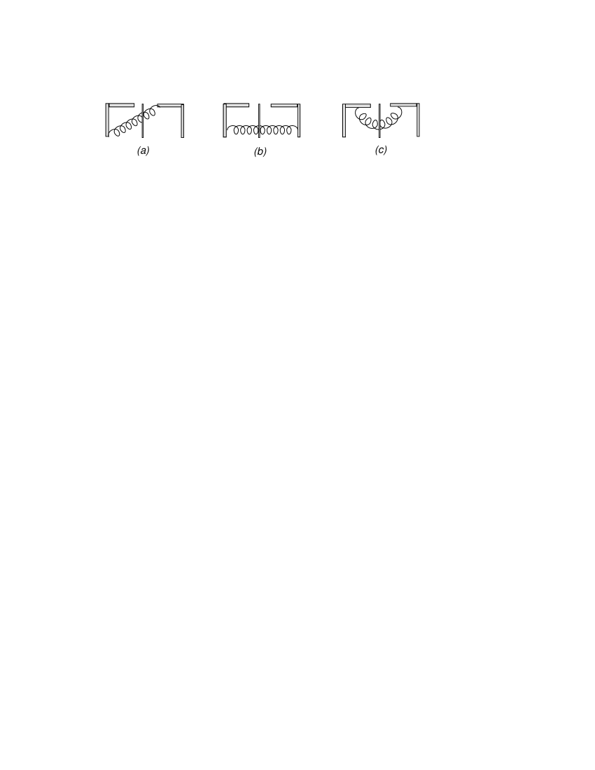
where ${\tilde{p}}=Q/{\sqrt{2}}$. The pre-factor is chosen to normalize the leading contribution to $\delta(1-x)$. The Feynman diagrams with real gluon emission that contribute to $S(1-x)$ are given in Fig. 2. Figs. 2(b) and 2(c) are identically zero due to $n^{2}={\bar{n}}^{2}=0$ respectively. The contribution from Fig. 2(a) is

$$S^{(a)}(1-x) = 2\alpha_{s}C_{F}(\mu^{2})^{\varepsilon}{\tilde{p}}\int\frac{d^{d}k}{(2\pi)^{d-2}}\frac{1}{k^{+}k^{-}}\delta(k^{2})\delta(k^{+}-(1-x){\tilde{p}})$$ (46)

$$=\frac{\alpha_{s}}{4\pi}C_{F}\left(\frac{\mu^{2}}{Q^{2}}\right)^{\varepsilon}\left[-\frac{1}{\varepsilon_{\text{IR}}}\delta(1-x)+D_{0}(x)\right]\left(\frac{2}{\varepsilon_{\text{UV}}}-\frac{2}{\varepsilon_{\text{IR}}}\right)\,\,,$$

and the $Q^{2}$-dependence is again put by hand as the integral is scaleless. We use $D_{i}(x)$ for the “plus” distributions:

$$D_{i}(x)\equiv\left[\frac{\ln^{i}(1-x)}{1-x}\right]_{+}\,\,\,\,\,i=0,1.$$ (47)

In going from the first to second line in Eq. (46) we have carried out the integral over $k^{+}$ first, then integrated over the transverse momentum, and finally integrated $k^{-}$ from $0$ and $\infty$. Taking the contribution from the mirror diagram of (a) and adding $2I_{s}\times\delta(1-x)$ ($I_{s}$ is given in Eq. (45)) to include the virtual contributions we get the soft factor to $O(\alpha_{s})$ in pure DR:

$$S(1-x) = \delta(1-x)$$

$$+\frac{\alpha_{s}}{4\pi}C_{F}\left(\frac{\mu^{2}}{Q^{2}}\right)^{\varepsilon}\times 4\left[\left(-\frac{1}{\varepsilon_{\text{UV}}^{2}}+\frac{1}{\varepsilon_{\text{UV}}\varepsilon_{\text{IR}}}\right)\delta(1-x)+D_{0}(x)\left(\frac{1}{\varepsilon_{\text{UV}}}-\frac{1}{\varepsilon_{\text{IR}}}\right)\right]\,\,.$$

The renormalized soft function to $O(\alpha_{s})$ is

$$S_{R}(1-x)=\delta(1-x)+\frac{\alpha_{s}}{4\pi}C_{F}\times(-4)\frac{D_{0}(x)}{\varepsilon_{\text{IR}}}\,\,.$$ (49)

Figure 2: Real gluon contribution to the soft factor.

Now we consider the PDF. Our definition of the PDF is analogous to the standard one in QCD col however it is expressed in terms of the naive collinear SCET fields,

$${\hat{\phi}}(x)=\frac{1}{2}\int\frac{d\lambda}{2\pi}e^{i\lambda x\!{\tilde{p}}}\langle P|\overline{{\hat{\xi}}}_{n}(\lambda{\bar{n}}){\hat{W}}_{n}(\infty,0;\lambda{\bar{n}})\times\gamma^{+}{\hat{W}}^{\dagger}_{n}(\infty,0;0){\hat{\xi}}_{n}(0)|P\rangle\,.$$ (50)

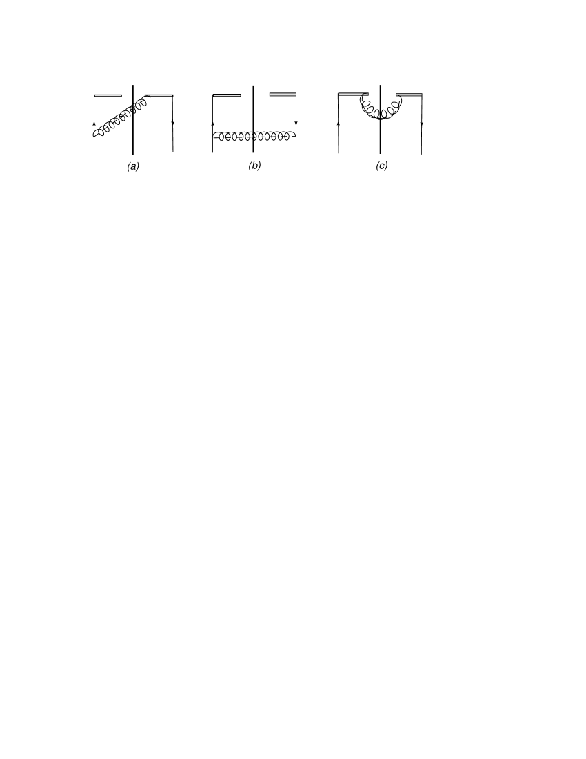
The Feynman diagrams with real gluon emission that contribute to the partonic PDF are given in Fig. 3.

Figure 3: Real gluon contribution to the PDF.

The contribution from Fig. 3(c) is again identically zero due to ${\bar{n}}^{2}=0$. The contribution from Fig. 3(b) is nonsingular in the limit $x\rightarrow 1$. Its contribution should be omitted since it is subleading in the SCET expansion parameter, $\lambda$, which for DIS in the threshold region has to be taken as $\lambda^{2}\cong 1-x$. The remaining contribution from Fig. 3(a) is given by:

$${\hat{\phi}}^{(a)}(x) = 2\alpha_{s}C_{F}(\mu^{2})^{\varepsilon}\int\frac{d^{d}k}{(2\pi)^{d-2}}\frac{{\tilde{p}}-k^{+}}{k^{+}k^{-}}\delta(k^{2})\delta(k^{+}-(1-x){\tilde{p}})$$ (51)

$$=\frac{\alpha_{s}}{4\pi}C_{F}\left(\frac{\mu^{2}}{Q^{2}}\right)^{\varepsilon}x\left[-\frac{1}{\varepsilon_{\text{IR}}}\delta(1-x)+D_{0}(x)\right]\left(\frac{2}{\varepsilon_{\text{UV}}}-\frac{2}{\varepsilon_{\text{IR}}}\right)\,\,.$$

Comparing the last result with the contribution from Fig. 2(a) given in Eq. (46) we see that in the $x\to 1$ limit both contributions are identical.

For the PDF the leading contribution in the $x\to 1$ limit (or equivalently in $\lambda$) comes entirely from the zero-bin region as we can see from the second $\delta$-function in Eq. (51). $k^{+}$ which is supposed to be $O(Q)$ (since $k$ is collinear to the incoming parton momentum with $p_{1}^{+}={\tilde{p}}=Q/{\sqrt{2}}$) is restricted to be equal to $(1-x){\tilde{p}}$ which is $O(Q\lambda^{2})$. Since $k^{-}$ is also $O(Q\lambda^{2})$ then the first $\delta$-function enforces the transverse components to be $O(Q\lambda^{2})$. Thus the contribution comes from the zero-bin (soft) region. Notice that Fig. 3(a) is the only diagram relevant to the PDF as $x\rightarrow 1$ because we have defined our PDF with the naive collinear fields, which allowed us to integrate over all momentum space including the zero-bin region. If we had restricted the SCET definition of the PDF to contain the purely collinear fields (i.e., so $k^{+}$ is $O(Q)$) then Fig. 3(a) would not contribute as the second $\delta$-function in Eq. (51) could not be satisfied by power counting arguments. Existing SCET treatments of DIS in the $x\to 1$ limit differ in their treatment of Fig. 3(a) Becher:2006mr ; Chay:2005rz . Ref. Becher:2006mr drops this diagram and argues that collinear modes cannot contribute because of kinematic constraints. This is essentially equivalent to our argument above that the diagram receives support only from modes whose scaling is soft rather than collinear. In our approach this contribution is removed from the purely collinear jet function by a zero-bin subtraction. Our purely collinear PDF (i.e. the naively evaluated PDF minus the zero-bin subtraction) is analogous to the function $g_{P}$ that appears in the factorization theorem of Ref. Chay:2005rz . However, zero-bin subtractions are required for both the PDF and the jet function, as we will see below, whereas Ref. Chay:2005rz only includes a zero-bin subtraction in their evaluation of the PDF.

The final state jet function represents outgoing (in the $\bar{n}$ direction) collinear partons with invariant mass $Q^{2}(1-x)$, which is assumed to be much larger than $\Lambda^{2}_{\rm QCD}$. To define the jet function, we start with the following two-point correlation function of collinear fields Bauer:2001yt

$$\langle 0|T\left[{\hat{W}}_{{\bar{n}}}^{\dagger}(z){\hat{\xi}}_{{\bar{n}}}(z)\bar{\hat{\xi}}_{{\bar{n}}}(0){\hat{W}}_{{\bar{n}}}(0)\right]|0\rangle=i\frac{\not\!{{\bar{n}}}}{\sqrt{2}}\int\frac{d^{4}k}{(2\pi)^{4}}e^{-ikz}{\hat{\cal J}}(k)\,\,.$$ (52)

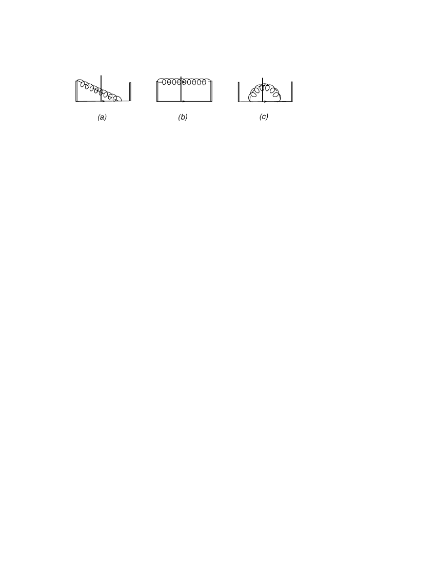
The naive dimensionless jet function, to be denoted by ${\hat{J}}(Q^{2},x)$, is related to the absorptive part of ${\hat{\cal J}}$ and normalized at leading order to $\delta(1-x)$, so that ${\hat{J}}(Q^{2},x)=\frac{-1}{\pi}{\tilde{p}}\times\mathrm{Im}{\hat{\cal J}}$. This definition is the gauge invariant version of the jet function defined in Ref. Sterman:1986aj with the full QCD fields replaced by the naive SCET ones. The Feynman diagrams with real gluon emission that contribute to the jet function are given in Fig. 4.

Figure 4: Real gluon contribution to the outgoing jet function.

The contribution of Fig. 4(c) is zero due to ${\bar{n}}^{2}=0$. From Fig. 4(a) we have

$${\hat{J}}^{(a)}(Q^{2},x) = \alpha_{s}C_{F}(\mu^{2})^{\varepsilon}\int\frac{d^{d}k}{(2\pi)^{d-2}}\frac{8{\tilde{p}}l^{-}}{k^{-}l^{2}}(l^{-}-k^{-})\delta(k^{2})\delta((l-k)^{2})$$ (53)

where $l$ is the momentum for the outgoing jet, whose components are $l^{+}=\frac{Q}{\sqrt{2}}(1-x)$; $l^{-}=\frac{Q}{\sqrt{2}}$ and $l_{\perp}=0$. $k$ is collinear to the outgoing quark momentum with $k^{-}\cong Q$, $k^{+}\cong Q\lambda^{2}$ and $k_{\perp}\cong Q\lambda$. Recalling that in threshold region for DIS we identify $1-x\cong\lambda^{2}$ then simple power counting shows that the above contribution scales as $1/\lambda^{2}$. Carrying out the integrations over $k^{+}$, $k_{\perp}$, and $k^{-}$ (in that order) we find

$${\hat{J}}^{(a)}(Q^{2},x) = \frac{\alpha_{s}}{4\pi}C_{F}\times 4\left[\left(\frac{1}{\varepsilon_{\text{IR}}^{2}}+\frac{1-\ln\left(\frac{Q^{2}}{\mu^{2}}\right)}{\varepsilon_{\text{IR}}}\right)\delta(1-x)-\frac{D_{0}(x)}{\varepsilon_{\text{IR}}}-D_{0}(x)+D_{1}(x)\right.$$ (54)

$$\left.+\left(\frac{1}{2}\ln^{2}\left(\frac{Q^{2}}{\mu^{2}}\right)-\ln\left(\frac{Q^{2}}{\mu^{2}}\right)+2-\frac{\pi^{2}}{4}\right)\delta(1-x)+\ln\left(\frac{Q^{2}}{\mu^{2}}\right)D_{0}(x)\right]\,\,,$$

The contribution from Fig. 4(c) can be obtained in similar manner and is given by

$${\hat{J}}^{(c)}(Q^{2},x) = \frac{\alpha_{s}}{4\pi}C_{F}\left[-\frac{\delta(1-x)}{\varepsilon_{\text{IR}}}-\left(1-\ln\left(\frac{Q^{2}}{\mu^{2}}\right)\right)\delta(1-x)+D_{0}(x)\right]\,\,,$$ (55)

Including the contribution from the mirror of Fig. 4(a) we get for the real gluon contribution to the jet function

$${\hat{J}}_{\rm real}(Q^{2},x) = \frac{\alpha_{s}}{4\pi}C_{F}\left[\left(\frac{4}{\varepsilon_{\rm IR}^{2}}+\frac{3-4\ln\left(\frac{Q^{2}}{\mu^{2}}\right)}{\varepsilon_{\rm IR}}\right)\delta(1-x)-\frac{4D_{0}(x)}{\varepsilon_{\rm IR}}+4D_{1}(x)\right.$$

$$\left.+4\ln\left(\frac{Q^{2}}{\mu^{2}}\right)D_{0}(x)+\left(2\ln^{2}\left(\frac{Q^{2}}{\mu^{2}}\right)-3\ln\left(\frac{Q^{2}}{\mu^{2}}\right)+7-\pi^{2}\right)\delta(1-x)\right]\,\,.$$

Let us now consider the zero-bin contribution included in the above result. For Fig. 4(a) we take the gluon momentum $k$ to be soft. Then we ignore $k^{-}$ relative $l^{-}$ in the numerator of Eq. (53) and we drop $k^{2}$ in the last $\delta$-function as it scales as $\lambda^{4}$ compared with $l^{2}\cong Q^{2}\lambda^{2}$. We then get a contribution that also scales as $1/\lambda^{2}$ like in the collinear region:

$$J_{\rm zb}^{(a)}(Q^{2},x) = 2\alpha_{s}C_{F}(\mu^{2})^{\varepsilon}\frac{1}{1-x}\int\frac{d^{d}k}{(2\pi)^{d-2}}\frac{1}{k^{-}}\delta(k^{2})\delta(k^{+}-l^{+})$$ (57)

$$=\frac{\alpha_{s}}{4\pi}C_{F}\left(\frac{\mu^{2}}{Q^{2}}\right)^{\varepsilon}\left[-\frac{1}{\varepsilon_{\text{IR}}}\delta(1-x)+D_{0}(x)\right]\left(\frac{2}{\varepsilon_{\text{UV}}}-\frac{2}{\varepsilon_{\text{IR}}}\right)\,\,,$$

The last result is exactly the same as the ones given in Eq. (46) and Eq. (51) (when taken to the $x\to 1$ limit.) Noticing that the zero-bin contribution from Fig. 4(b) is subleading in $\lambda$ so the soft contribution to the real gluon emission for the jet function comes only from Fig. 4(a).

We now include the virtual contributions to the soft factor, PDF and jet function. For the soft factor the only contribution comes from Fig. 1(c). The sum of the real and virtual contributions is

$$S(1-x)=\delta(1-x)+\frac{\alpha_{s}}{4\pi}C_{F}\times 4\left(\frac{1}{\varepsilon_{\text{UV}}}-\frac{1}{\varepsilon_{\text{IR}}}\right)\left[-\frac{1}{\varepsilon_{\text{UV}}}\delta(1-x)+D_{0}(x)\right]\,\,.$$ (58)

Note that the soft function is scaleless and the final answer is proportional to $\frac{1}{\varepsilon_{\text{UV}}}-\frac{1}{\varepsilon_{\text{IR}}}$. The factor $(\mu^{2}/Q^{2})^{\epsilon}$ can be set to unity since when we expand this factor in powers of $\epsilon$ and mulitply by $\frac{1}{\varepsilon_{\text{UV}}}-\frac{1}{\varepsilon_{\text{IR}}}$, the finite logarithms cancel. This makes physical sense since this quantity is scaleless. A similar situation arises for the PDF, $\hat{\phi}(x)$, however, the jet function will have logarithms of $Q$ because it knows about the scale $Q\sqrt{1-x}$. The renormalized soft function to $O(\alpha_{s})$ is

$$S^{R}(1-x)=\delta(1-x)+\frac{\alpha_{s}}{4\pi}C_{F}\times(-4)\frac{D_{0}(x)}{\varepsilon_{\text{IR}}}\,\,.$$ (59)

The large $N$ moments of the soft function are

$$S^{R}_{N}=1+\frac{\alpha_{s}}{4\pi}C_{F}\times 4\frac{\ln{\overline{N}}}{\varepsilon_{\text{IR}}}\,\,,$$ (60)

with $\ln{\overline{N}}=Ne^{\gamma_{E}}$. For the PDF, after including virtual contributions, we find

$${\hat{\phi}}(x)=\delta(1-x)+\frac{\alpha_{s}}{4\pi}C_{F}\left[3\left(\frac{1}{\varepsilon_{\text{UV}}}-\frac{1}{\varepsilon_{\text{IR}}}\right)\delta(1-x)+4D_{0}(x)\left(\frac{1}{\varepsilon_{\text{UV}}}-\frac{1}{\varepsilon_{\text{IR}}}\right)\right]\,\,.$$ (61)

The renormalized PDF is

$${\hat{\phi}}^{R}(x)=\delta(1-x)+\frac{\alpha_{s}}{4\pi}C_{F}\left(-\frac{1}{\varepsilon_{\text{IR}}}\right)\left[3\delta(1-x)+4D_{0}(x)\right]\,\,,$$ (62)

and in moment space we get

$${\hat{\phi}}^{R}_{N}=1+\frac{\alpha_{s}}{4\pi}C_{F}\left(-\frac{1}{\varepsilon_{\text{IR}}}\right)\left[3-4\ln{\overline{N}}\right]\,\,,$$ (63)

which is a well-known result. The anomalous dimension of the (naive) PDF can be immediately read off from the UV poles in Eq. (61) :

$$\gamma_{2,N}=\frac{\alpha_{s}}{4\pi}C_{F}\times 2[4\ln{\overline{N}}-3]\,\,.$$ (64)

The virtual contribution to the jet function comes from Fig. 1(b), its mirror diagram, and the wave function renormalization. In the result for $I_{\bar{n}}$ (which is equal to $I_{n}$ given in Eq. (34)) we expand the factor $(\mu^{2}/Q^{2})^{\varepsilon}$ and get for the naive jet function

$${\hat{J}}(Q^{2},x) = \delta(1-x)+\frac{\alpha_{s}}{4\pi}C_{F}\left[-\frac{4D_{0}(x)}{\varepsilon_{\text{IR}}}+4D_{1}(x)+4\ln\left(\frac{Q^{2}}{\mu^{2}}\right)D_{0}(x)\right.$$ (65)

$$\left.+\left(2\ln^{2}\left(\frac{Q^{2}}{\mu^{2}}\right)-3\ln\left(\frac{Q^{2}}{\mu^{2}}\right)+7-\pi^{2}\right)\delta(1-x)\right]$$

$$+\frac{\alpha_{s}}{4\pi}C_{F}\left(\frac{\mu^{2}}{Q^{2}}\right)^{\varepsilon}\left[\frac{4}{\varepsilon_{\text{UV}}\varepsilon_{\text{IR}}}+\frac{3}{\varepsilon_{\text{UV}}}\right]\delta(1-x)\,\,.$$

Next we have to include the zero-bin subtraction which as we have seen earlier is equivalent to subtracting the one-loop soft contribution. It is easy to see the effect of the zero-bin subtraction is to replace $1/\epsilon_{\rm IR}$ everywhere in Eq. (65) with $1/\epsilon_{\rm UV}$. The remaining UV divergences can now be removed by counterterms and the renormalized jet function is

$${J}^{R}(Q^{2},x) = \delta(1-x)+\frac{\alpha_{s}}{4\pi}C_{F}\left[4D_{1}(x)+4\ln\left(\frac{Q^{2}}{\mu^{2}}\right)D_{0}(x)\right.$$ (66)

$$\left.+\left(2\ln^{2}\left(\frac{Q^{2}}{\mu^{2}}\right)-3\ln\left(\frac{Q^{2}}{\mu^{2}}\right)+7-\pi^{2}\right)\delta(1-x)\right]\,\,.$$

The results presented so far for the zero-bin contributions (real and virtual) for the naive PDF and jet function show that the renormalized soft factor has to be subtracted from each one of these functions to obtain the truly collinear contributions. Thus we find that the renormalized collinear matrix elements are

$$\phi^{R}_{N}=\left(\frac{{\hat{\phi}}_{N}}{S_{N}}\right)^{R}\,\,\,\,~{}~{}~{}~{}~{}J^{R}_{N}=\left(\frac{{\hat{j}}_{N}}{S_{N}}\right)^{R}\,\,,$$ (67)

which to $O(\alpha_{s})$ are given by

$$\phi^{R}_{N}=1+\frac{\alpha_{s}}{4\pi}C_{F}\times(-3)\frac{1}{\varepsilon_{\text{IR}}}\,\,,$$ (68)

and

$$J_{N}^{R}=1+\frac{\alpha_{s}}{4\pi}C_{F}\left[2\ln^{2}\left(\frac{Q^{2}}{\overline{N}\mu^{2}}\right)-3\ln\left(\frac{Q^{2}}{\overline{N}\mu^{2}}\right)+7-\frac{2}{3}\pi^{2}\right]\,\,.$$ (69)

The last result for the collinear jet is finite and is equal to the matching coefficient for DIS at the intermediate scale, $\mu^{2}=Q^{2}/{\overline{N}}$, in the analysis of DIS as $x\to 1$ in Ref. Manohar:2003vb . Thus the factorization theorem for DIS in the threshold region reads

$$F_{2,N}=H(Q^{2}/\mu^{2})\,J^{R}_{N}\,\phi^{R}_{N}\,S^{R}_{N}=H(Q^{2}/\mu^{2})\left(\frac{{\hat{J}}_{N}}{S_{N}}\right)^{R}\left(\frac{{\hat{\phi}}_{N}}{S_{N}}\right)^{R}S^{R}_{N}\,\,.$$ (70)

where $H(Q^{2}/\mu^{2})$ is the square of the matching coefficient $C(Q^{2}/\mu^{2})$ given in Eq. (28). With the above results for $J^{R}_{N}$, $\phi^{R}_{N}$ and $S^{R}_{N}$ we get

$$H(Q^{2}/\mu^{2})\,J^{R}_{N}\,\phi^{R}_{N}\,S^{R}_{N} = 1+\frac{\alpha_{s}}{4\pi}C_{F}\left\{-\frac{1}{\varepsilon_{\text{IR}}}[3-4\ln{\overline{N}}]-2\ln^{2}\left(\frac{Q^{2}}{\mu^{2}}\right)+6\ln\left(\frac{Q^{2}}{\mu^{2}}\right)\right.$$ (71)

$$\left.+2\ln^{2}\left(\frac{Q^{2}}{{\overline{N}}\mu^{2}}\right)-3\ln\left(\frac{Q^{2}}{{\overline{N}}\mu^{2}}\right)-9-\frac{\pi^{2}}{3}\right\}\,\,,$$

which agrees with the moments of DIS structure function in the large-$N$ limit calculated in full QCD. It is straightforward to show that the results in Eq. (67) which were shown to hold to ${\cal O}(\alpha_{s})$ in pure DR can be obtained by performing field redefinitions Lee:2006nr on the naive SCET fields and one obtains the naive collinear matrix elements divided by the soft Wilson line matrix elements as in Eq. (3).

Based on the factorized form of the non-singlet DIS structure function given in Eq. (70) we now comment on the resummation of the large logarithms in the threshold region for DIS. In moment space Eq. (70) can be written in the following form (henceforth we drop the superscript $R$ with the understanding that we consider only renormalized quantities)

$$F_{2,N}=H(Q^{2}/\mu^{2})J_{N}\left(\frac{Q^{2}}{{\overline{N}}\mu^{2}}\right)\hat{\phi}_{N}(\mu^{2})\,\,.$$ (72)

The hard part $H$ depends only on $Q^{2}/\mu^{2}$ and it is obtained by matching the full QCD current onto the SCET one (at the higher scale $Q^{2}$) order by order in perturbation theory. The anomalous dimension of the SCET current $\gamma_{1}$ is then calculated from the matching coefficient (through Eq. (29)) and is used to run down to the intermediate scale of DIS: $Q^{2}/{\overline{N}}$. The quantity $J_{N}$, which is IR safe, depends only on the intermediate scale as can be seen in Eq.(69). Thus the first two terms on the right hand side of Eq. (72) are perturbative and IR safe. Below the intermediate scale we are left with only one non-perturbative quantity, the PDF taken to the large $N$ limt. By exploiting the standard Altarelli-Parisi kernels with anomalous dimension $\gamma_{2}$ (taken to the large $N$-limit) we can then evolve the PDF to an arbitrary factorization scale. The two stage running between $Q^{2}$ and $Q^{2}/{\overline{N}}$ with $2\gamma_{1}$ and between $Q^{2}/{\overline{N}}$ and some arbitrary factorization scale $\mu_{F}$ with $\gamma_{2}$ resums all the large logarithms in moment space. This has been established to be equivalent to the standard pQCD resummation Sterman:1986aj ; Catani:1989ne in Ref. Idilbi:2006dg to all orders in the strong coupling constant and to arbitrary sub-leading logarithms.

IV Zero-Bin At Higher Orders

In this section we consider the abelian virtual two-loop diagrams that contribute to the $n$-collinear jet function $\langle 0|W^{(0)\dagger}_{n}\xi^{(0)}_{n}|q(p)\rangle$ that appears in the factorization theorem for the quark form factor. We will show how dividing by the soft factor reproduces the zero-bin subtraction for these diagrams.

The abelian two-loop diagrams are shown in Fig. 6. Before considering these in detail we make some general comments about the zero-bin subtraction at two loops. Let $k_{1}$ and $k_{2}$ be the loop momenta, which are routed so that $k_{1}$ and $k_{2}$ correspond to the virtual gluon momenta, since the zero-bin associated with any fermion lines is easily checked to be subleading in the $\lambda$ expansion. Since we integrate over all momentum space, we need to subtract the contribution where either of the $k_{i}$ scales like a soft momentum rather than collinear. 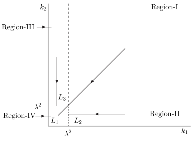In Fig. 5, the region where $k_{1}$ ($k_{2}$) is collinear is separated from the region where $k_{1}$ ($k_{2}$) is soft by the vertical (horizontal) dotted line.

Figure 5: Zero-Bin Regions At Two-Loops.

The collinear matrix element gets contributions only from Region-I. Region-II corresponds to $k_{2}$ soft and $k_{1}$ collinear, Region-III corresponds to $k_{1}$ soft and $k_{2}$ collinear, and Region-IV corresponds to both $k_{1}$ and $k_{2}$ soft.

Denote the integrand of the two-loop integral ${\cal I}(k^{c}_{1},k^{c}_{2})$, where the superscript $c$ in $k_{i}^{c}$ means that $k_{i}$ is assumed to have collinear scaling. The naive two-loop integral is

$$(\mu^{2})^{2\epsilon}\int\frac{d^{d}k_{1}}{(2\pi)^{d}}\int\frac{d^{d}k_{2}}{(2\pi)^{d}}{\cal I}(k^{c}_{1},k^{c}_{2})\equiv\int_{k_{1},k_{2}}{\cal I}(k^{c}_{1},k^{c}_{2})\,.$$ (73)

The integrands for the zero-bin subtractions for Region-II and Region-III are $-{\cal I}(k^{c}_{1},k^{s}_{2})$ and $-{\cal I}(k^{s}_{1},k^{c}_{2})$, respectively, where the superscript $s$ in $k_{i}^{s}$ means that the integrand is evaluated assuming that $k_{i}$ satisfies the soft scaling and the integrand is expanded to lowest order in $\lambda$. The zero-bin subtraction from Region-IV is subtle because this Region has been doubly counted both in the original naive collinear integrals and also in the zero-bin subtraction for Region-II and Region-III. From the original integral we need to subtract a contribution in which both $k_{1}$ and $k_{2}$ are soft. We will denote the integrand for this zero-bin as ${\cal I}_{L_{1}}(k^{s}_{1},k^{s}_{2})$, where $L_{1}$ denotes the limit when $k_{1}$ and $k_{2}$ are taken to be soft simultaneously. From the zero-bin subtraction for Region-II, we must perform a second subtraction that comes from $k_{1}^{c}$ becoming soft after having first made the soft approximation for $k_{2}$. We call the integrand for the zero-bin subtraction defined by this limit ${\cal I}_{L_{2}}(k_{1}^{s},k_{2}^{s})$. Likewise, we have a similar subtraction from the zero-bin of Region-III, denoted ${\cal I}_{L_{3}}(k_{1}^{s},k_{2}^{s})$. In general, the integrand ${\cal I}_{L_{i}}(k_{1}^{s},k_{2}^{s})$ depends on the order in which we take the soft limits, so there are really five different zero-bin subtractions in the two-loop calculation. The result for the collinear contribution to each two-loop diagram is

$$\int_{k_{1},k_{2}}\left({\cal I}(k_{1}^{c},k_{2}^{c})-\bigg{[}{\cal I}(k_{1}^{c},k_{2}^{s})-{\cal I}_{L_{2}}(k_{1}^{s},k_{2}^{s})\bigg{]}-\bigg{[}{\cal I}(k_{1}^{s},k_{2}^{c})-{\cal I}_{L_{3}}(k_{1}^{s},k_{2}^{s})\bigg{]}-{\cal I}_{L_{1}}(k_{1}^{s},k_{2}^{s})\right)\,.$$ (74)

The various order of limits defining the integrands ${\cal I}_{L_{i}}(k_{1}^{s},k_{2}^{s})$ are shown in Fig. 5.

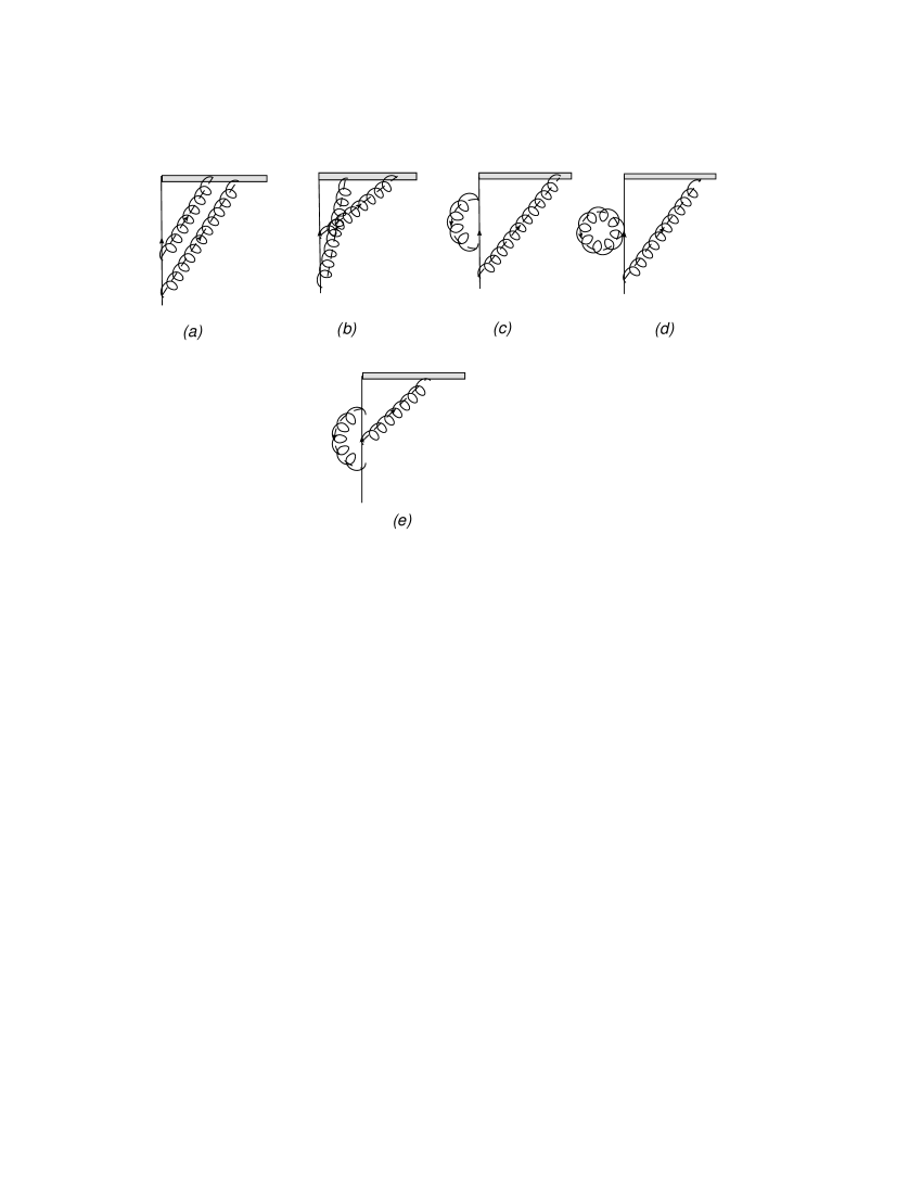
Figure 6: All the two-loop abelian diagrams that contribute the $n$-collinear jet function.

Next we turn to the evaluation of the individual diagrams. Figs. 6(a) 6(c) and 6(d) have color factors proportional to $C_{F}^{2}$ while the color factors for Figs. 6(b) and 6(e) are $C_{F}(C_{F}-C_{A}/2)$. The results for an abelian theory are obtained by taking $C_{F}\to 1$ and $C_{A}\to 0$, in which case the color factor is one for all graphs in Fig. 6.

Consider first the two-loop SCET diagrams in Fig. 6(a) and 6(b). Working in Feynman gauge, using pure DR as a regulator, and ignoring the $i\epsilon$’s in the propagators as they are not relevant to our discussion, we get from Fig. 6(a),

$$I^{(a)}=-2g_{s}^{4}\int_{k_{1},k_{2}}\frac{(p^{+}-k_{1}^{+}-k_{2}^{+})}{(p-k_{1}-k_{2})^{2}k_{1}^{2}k_{2}^{2}(k_{1}^{+}+k_{2}^{+})}\left[\frac{(p^{+}-k_{1}^{+})}{(p-k_{1})^{2}k_{1}^{+}}+\frac{(p^{+}-k_{2}^{+})}{(p-k_{2})^{2}k_{2}^{+}}\right]\ ,$$ (75)

where $k_{i}$ are both collinear to the incoming parton with momentum $p$. From Fig. 6(b) we have

$$I^{(b)}=-2g_{s}^{4}\int_{k_{1},k_{2}}\frac{(p^{+}-k_{1}^{+}-k_{2}^{+})}{(p-k_{1}-k_{2})^{2}k_{1}^{2}k_{2}^{2}(k_{1}^{+}+k_{2}^{+})}\left[\frac{(p^{+}-k_{1}^{+})}{(p-k_{1})^{2}k_{2}^{+}}+\frac{(p^{+}-k_{2}^{+})}{(p-k_{2})^{2}k_{1}^{+}}\right]\ ,$$ (76)

In Eqs. (75) and (76), we have chosen to write the integrand so it is symmetric under interchange of $k_{1}$ and $k_{2}$.

The integrands for Figs. 6(a) and 6(b) in Region-IV are

$${\cal I}_{L_{1}}^{(a)}(k_{1}^{s},k_{2}^{s})=-g_{s}^{4}\frac{1}{2}\frac{1}{k_{1}^{2}k_{2}^{2}(k_{1}^{-}+k_{2}^{-})(k_{1}^{+}+k_{2}^{+})}\left[\frac{1}{k_{1}^{-}k_{1}^{+}}+\frac{1}{k_{2}^{-}k_{2}^{+}}\right]\,\,,$$ (77)

and

$${\cal I}_{L_{1}}^{(b)}(k_{1}^{s},k_{2}^{s})=-g_{s}^{4}C_{F}^{2}\times\frac{1}{2}\frac{1}{k_{1}^{2}k_{2}^{2}(k_{1}^{-}+k_{2}^{-})(k_{1}^{+}+k_{2}^{+})}\left[\frac{1}{k_{1}^{-}k_{2}^{+}}+\frac{1}{k_{2}^{-}k_{1}^{+}}\right]\,\,.$$ (78)

Note that the contributions in Eq. (77) and Eq. (78) are not subleading in SCET power counting. For the two loop momenta in the soft region, the measure of the loop integral scales as $\lambda^{16}$ and each integrand scales as $1/{\lambda^{16}}$ thus the contribution is ${\cal O}(1)$. The sum of these two zero-bin contributions is

$$\int_{k_{1},k_{2}}\left({\cal I}_{L_{1}}^{(a)}(k^{s}_{1},k^{s}_{2})+{\cal I}_{L_{1}}^{(b)}(k^{s}_{1},k^{s}_{2})\right)=-g_{s}^{4}\int_{k_{1},k_{2}}\frac{1}{2}\frac{1}{(k_{1}^{2}k_{1}^{-}k_{1}^{+})(k_{2}^{2}k_{2}^{-}k_{2}^{+})}=\frac{1}{2}I^{2}_{s}\,\,,$$ (79)

where $I_{s}$ is the one-loop soft contribution given in Eq. (16). The two-loop result is consistent with the exponentiation theorem for the abelian amplitudes of soft gluon radiation in a web (i.e., two soft Wilson lines).

Now we consider the case when one collinear momentum becomes soft while the other is kept collinear. In Eq. (77) let us take $k_{1}$ to the zero-bin region. The integrand is then

$${\cal I}^{(a)}(k_{1}^{s},k^{c}_{2})=-2g_{s}^{4}\frac{(p^{+}-k_{2}^{+})}{[(p-k_{2})^{2}-2k_{1}^{-}(p^{+}-k_{2}^{+})]k_{1}^{2}k_{2}^{2}k_{2}^{+}}\left[\frac{p^{+}-k_{2}^{+}}{(p-k_{2})^{2}k_{2}^{+}}+\frac{1}{-2k_{1}^{-}k_{1}^{+}}\right]\,\,.$$ (80)

The measure in the loop integral in this case scales as $\lambda^{12}$ because there is one collinear and one soft loop momentum. The factor outside the brackets in the integrand scales as $\lambda^{-8}$, the first factor inside square brackets scales as $\lambda^{-2}$ and the second scales as $\lambda^{-4}$. Therefore, only the second term contributes so we get

$${\cal I}^{(a)}(k_{1}^{s},k_{2}^{c})=-2g_{s}^{4}\frac{(p^{+}-k_{2}^{+})}{[(p-k_{2})^{2}-2k_{1}^{-}(p^{+}-k_{2}^{+})]k_{1}^{2}k_{2}^{2}k_{2}^{+}}\left[\frac{1}{-2k_{1}^{-}k_{1}^{+}}\right]\,\,.$$ (81)

Similarly for $k_{1}$ collinear and $k_{2}$ soft we find

$${\cal I}^{(a)}(k_{1}^{c},k_{2}^{s})=-2g_{s}^{4}\frac{(p^{+}-k_{1}^{+})}{[(p-k_{1})^{2}-2k_{2}^{-}(p^{+}-k_{1}^{+})]k_{1}^{2}k_{2}^{2}k_{1}^{+}}\left[\frac{1}{-2k_{2}^{-}k_{2}^{+}}\right]\,\,.$$ (82)

The analogous zero-bins for Fig. 6(b) are

$${\cal I}^{(b)}(k_{1}^{s},k_{2}^{c})=-2g_{s}^{4}\frac{(p^{+}-k_{2}^{+})}{[(p-k_{2})^{2}-2k_{1}^{-}(p^{+}-k_{2}^{+})]k_{1}^{2}k_{2}^{2}k_{2}^{+}}\left[\frac{p^{+}-k_{2}^{+}}{(p-k_{2})^{2}k_{1}^{+}}\right]\,\,,$$ (83)

and

$${\cal I}^{(b)}(k_{1}^{c},k_{2}^{s})=-2g_{s}^{4}\frac{(p^{+}-k_{1}^{+})}{[(p-k_{1})^{2}-2k_{2}^{-}(p^{+}-k_{1}^{+})]k_{1}^{2}k_{2}^{2}k_{1}^{+}}\left[\frac{p^{+}-k_{1}^{+}}{(p-k_{1})^{2}k_{2}^{+}}\right]\,\,.$$ (84)

Upon summing the zero-bins for each Region, the integrand factorizes. For Region-II, we get

$${\cal I}^{(a)}(k_{1}^{c},k_{2}^{s})+{\cal I}^{(b)}(k_{1}^{c},k_{2}^{s})=g_{s}^{4}\,\frac{(p^{+}-k_{1}^{+})}{(p-k_{1})^{2}k_{1}^{2}k_{1}^{+}}\times\frac{1}{k_{2}^{2}k_{2}^{-}k_{2}^{+}}$$ (85)

and for Region-III we obtain the same with $k_{1}$ and $k_{2}$ interchanged. The zero-bins for Region-II and Region-III combine to give

$$\int_{k_{1},k_{2}}\left({\cal I}^{(a)}(k_{1}^{s},k_{2}^{c})+{\cal I}^{(a)}(k_{1}^{c},k_{2}^{s})+{\cal I}^{(b)}(k_{1}^{s},k_{2}^{c})+{\cal I}^{(b)}(k_{2}^{s},k_{1}^{c})\right)=I_{n}\cdot I_{s}\,\,,$$ (86)

where $I_{n}$ is the one-loop contribution to the $n$-collinear jet in Eq. (14). Finally, we have to perform the second zero-bin subtraction from the zero-bins corresponding to Region-II and Region-III, i.e. the terms with integrands ${\cal I}_{L_{2}}(k_{1}^{s},k_{2}^{s})$ and ${\cal I}_{L_{3}}(k_{1}^{s},k_{2}^{s})$ in Eq. (74). It is clear from Eq. (85) that this is simply $\frac{1}{2}I_{s}^{2}$ for each Region. Thus the final result for Figs. 6(a) and 6(b) including all zero-bin subtractions is

$$I^{(a)}+I^{(b)}-[I_{n}\cdot I_{s}-I_{s}^{2}]-\frac{1}{2}I_{s}^{2}=I^{(a)}+I^{(b)}-I_{n}\cdot I_{s}+\frac{1}{2}I_{s}^{2}\,\,,$$ (87)

where $I^{(a)}$ and $I^{(b)}$ correspond to the naive evaluation of Figs. 6(a) and 6(b), respectively.

Next we turn to the evaluation of Figs. 6(c)-(e). Denote the momentum that flows into the gluon attached to the collinear Wilson line as $k_{2}$ while the momentum flowing through the other gluon as $k_{1}$. For these three diagrams it is easy to show that the only zero-bin contribution which is leading in $\lambda$ comes from the region where $k_{1}$ is collinear and $k_{2}$ is soft. In Figs. 6(c) and (d), $k_{1}$ flows through the self-energy subgraph. The self-energy in the collinear sector of SCET is evaluated in Ref. Bauer:2001yt with the result that

$$\Sigma(q^{2})=\frac{\alpha_{s}}{4\pi}\frac{q^{2}}{2q^{+}}\frac{n\!\!\!/}{2}\frac{\Gamma(\epsilon)\Gamma(1-\epsilon)\Gamma(2-\epsilon)}{\Gamma(2-2\epsilon)}\left(\frac{-q^{2}}{e^{\gamma_{E}}\mu^{2}}\right)^{-\epsilon}\,,$$ (88)

where $q^{2}$ is the virtuality, which in our case is $q^{2}=(p-k_{2})^{2}=-2p^{+}k_{2}^{-}+{\cal O}(\lambda^{4})$. Inserting this result into the two-loop graphs in Figs. 6(c) and (d) yields the integral

$$\int_{k_{1},k_{2}}\left({\cal I}^{(c)}(k_{1}^{c},k_{2}^{s})+{\cal I}^{(d)}(k_{1}^{c},k_{2}^{s})\right)$$ (89)

$$\qquad=i\alpha_{s}^{2}\frac{\Gamma(\epsilon)\Gamma(1-\epsilon)\Gamma(2-\epsilon)}{\Gamma(2-2\epsilon)}({e^{\gamma_{E}}\mu^{4}})^{\epsilon}\int_{k_{2}}\frac{1}{k_{2}^{+}k_{2}^{-}k_{2}^{2}}(2p^{+}k_{2}^{-})^{-\epsilon}\,.$$

To evaluate Fig. 6(e), we perform the $k_{1}$ integral which is simply the collinear vertex correction in the limit that the external gluon is taken to be soft. Equivalently, this subgraph is simply the one-loop vertex correction to the coupling between the collinear quark and soft gluon. The result after doing this integral is

$$\int_{k_{1},k_{2}}{\cal I}^{(e)}(k_{1}^{c},k_{2}^{s})=-i\alpha_{s}^{2}\frac{\Gamma(\epsilon)\Gamma(1-\epsilon)\Gamma(2-\epsilon)}{\Gamma(2-2\epsilon)}({e^{\gamma_{E}}\mu^{4}})^{\epsilon}\int_{k_{2}}\frac{1}{k_{2}^{+}k_{2}^{-}k_{2}^{2}}(2p^{+}k_{2}^{-})^{-\epsilon}$$

We find that the zero-bins for Fig. 6(c),(d) and (e) add up to zero. The cancellation can be partly understood on the basis of the QED Ward identity, which relates the UV divergent pieces in the self-energy and vertex correction.

There are no zero-bin subtractions beyond those given in Eq. (87). We now compare this result with the soft subtraction, Eq. (12), which yields

$$\frac{\langle 0|\hat{W}^{\dagger}_{n}{\hat{\xi}}_{n}|q(p_{1})\rangle}{\langle 0|Y^{\dagger}_{\bar{n}}Y_{n}|0\rangle} = \frac{1+I_{n}+I^{(a)-(e)}+...}{1+I_{s}+\frac{1}{2}I_{s}^{2}+...}$$

$$= 1+(I_{n}-I_{s})+\left(I^{(a)-(e)}-I_{n}\cdot I_{s}+\frac{1}{2}I_{s}^{2}\right)+...\,.$$

In the right hand side of the first line, we have expanded the numerator and denominator to $O(\alpha_{s}^{2})$, separately. The one-loop naive collinear integral is $I_{n}$, $I^{(a)-(e)}$ is the naive collinear evaluation of the sum of graphs in Fig. 6, $I_{s}$ is the one-loop soft integral, and the second order term in the denominator is a consequence of the exponentiation theorem of the abelian contributions inside a web mentioned earlier. In the second line, we have expanded the quotient to second order in $\alpha_{s}$. The $O(\alpha_{s}^{2})$ term is consistent with Eq. (87) and the cancellation of the zero-bin in the sum of Figs.6(c),(d) and (e). Therefore, dividing by the soft Wilson line and the zero-bin subtraction give the same result. It would be interesting to extend the analysis of this section to the non-abelian theory.

V Conclusions

In this paper we have considered the two prescriptions deivsed to remove overlapping contributions to collinear matrix elements, the soft and zero-bin subtractions. We have demonstrated explicitly the equivalence of the two prescriptions for the abelian contributions to the quark form factor up to two-loop level using DR to regularize both UV and IR divergences. We also studied DIS in the threshold region to ${\cal O}(\alpha_{s})$ in SCET. In our treatment for DIS all Wilson lines were defined on the light-cone.The essential result is that soft contributions to naively defined collinear matrix elements have to be subtracted in order to derive proper factorization theorems as in Eq. (3). We have shown by explicit calculation that soft and zero-bin subtractions are equivalent in the examples studied in this paper. Our results obtained by fixed order pertubative calculations can be extended to all orders in the strong coupling by performing field redefinitions as proposed in Ref. Lee:2006nr with a suitable choice of IR regulators.

VI Appendix

Here we explain in detail why the poles in Eq. (22) are UV using contour integration. Let us first integrate over the light-cone component $k^{-}$ with contour integration. The poles are

$$k^{-}=\frac{|\vec{k}_{\perp}|^{2}}{2(k^{+}-{\tilde{p}})}-\frac{i0}{2(k^{+}-{\tilde{p}})},~{}~{}~{}~{}k^{-}=\frac{|\vec{k}_{\perp}|^{2}+2{\tilde{p}}k^{+}}{2k^{+}}-\frac{i0}{2k^{+}},~{}~{}~{}~{}k^{-}=i0.$$ (91)

There are two regions that contribute, $0\leq k^{+}\leq{\tilde{p}}$ and $k^{+}\geq{\tilde{p}}$. For $0\leq k^{+}\leq{\tilde{p}}$ we have to pick the second pole. For $k^{+}\geq{\tilde{p}}$ we have to pick the third pole. After performing the contour integration we integrate over $|\vec{k}_{\perp}|^{2}$ in $d=2-2\varepsilon$. This will introduce the first $\Gamma(\varepsilon_{\rm UV})$. We then integrate over $k^{+}$. For the contribution from $0\leq k^{+}\leq{\tilde{p}}$, the integration over $k^{+}$ will introduce another pole as $k^{+}\rightarrow 0$, $\Gamma(-\varepsilon)$. This pole has to be taken as UV for the following reason: When $k^{+}\rightarrow 0$, then from the second pole in Eq. (91) we see that $k^{-}\rightarrow\infty$. This combination clearly means that both $k^{0}$ and $k^{3}$ approach infinity (in addition to the UV pole from $|\vec{k}_{\perp}|^{2}\rightarrow\infty$). The same reasoning applies for the contribution from the region $k^{+}\geq{\tilde{p}}$ where we get $\Gamma(-\varepsilon)$ from $k^{+}\rightarrow\infty$. The third pole in Eq. (91) indicates $k^{-}\rightarrow 0$ so we again have one light-cone component approaching zero while the other one approaches infinity. Thus both contributions have a double UV poles and the total result is given in Eq. (22). The observation that a vanishing light-cone component may lead to a UV divergence (as opposed to IR divergence) was also discussed in Ref. Bauer:2003td .