Gluon-gluon contributions to the production of continuum diphoton pairs at hadron colliders

Abstract

We compute the contributions to continuum photon pair production at hadron colliders from processes initiated by gluon-gluon and gluon-quark scattering into two photons through a four-leg virtual quark loop. Complete two-loop cross sections in perturbative quantum chromodynamics are combined with contributions from soft parton radiation resummed to all orders in the strong coupling strength. The structure of the resummed cross section is examined in detail, including a new type of unintegrated parton distribution function affecting azimuthal angle distributions of photons in the pair’s rest frame. As a result of this analysis, we predict diphoton transverse momentum distributions in gluon-gluon scattering in wide ranges of kinematic parameters at the Fermilab Tevatron and the CERN Large Hadron Collider.

I Introduction

Advances in the computation of higher-order radiative contributions in perturbative quantum chromodynamics (PQCD) open opportunities to predict hadronic observables at an unprecedented level of precision. Full realization of this potential requires concurrent improvements in the methods for QCD factorization and resummation of logarithmic enhancements in hadronic cross sections in infrared kinematic regions. All-orders resummation of logarithmic corrections, such as the resummation of transverse momentum ($Q_{T}$) logarithms in Drell-Yan-like processes Collins et al. (1985), is increasingly challenging in multi-loop calculations as a result of algebraic complexity and new types of logarithmic singularities associated with multi-particle matrix elements.

In this paper, we address new theoretical issues in $Q_{T}$ resummation at two-loop accuracy. We focus on photon pair production, particularly on the gluon-gluon subprocess, $gg\rightarrow\gamma\gamma$, one of the important short-distance subprocesses that contribute to the inclusive reactions $p\bar{p}\rightarrow\gamma\gamma X$ at the Fermilab Tevatron and $pp\rightarrow\gamma\gamma X$ at the CERN Large Hadron Collider (LHC). This hadronic reaction is interesting in its own right, and it is relevant in searches for the Higgs boson $h$, where it constitutes an important QCD background to the $pp\rightarrow hX\rightarrow\gamma\gamma X$ production chain ATLAS Collaboration (1999); CMS Collaboration (2006); Abdullin et al. (2005). A reliable prediction of the cross section for $gg\rightarrow\gamma\gamma$ is needed for complete estimates of the $\gamma\gamma$ production cross sections, a task that we pursue in accompanying papers Balazs et al. (2006, 2007).

The lowest-order contribution to the cross section for $gg\rightarrow\gamma\gamma$ arises from a $2\rightarrow 2$ diagram of order ${\mathcal{O}}(\alpha^{2}\alpha_{s}^{2})$ involving a 4-vertex virtual quark loop [Fig. 1(a)]. We evaluate all next-to-leading (NLO) contributions of order ${\mathcal{O}}(\alpha^{2}\alpha_{s}^{3})$ to the $gg\rightarrow\gamma\gamma$ process shown in Figs. 1(b-e). An important new ingredient in this paper is the inclusion of the $gq\rightarrow\gamma\gamma q$ process, Fig. 1(d), a necessary component of the resummed NLO contribution. Our complete treatment of the NLO cross section represents an improvement over our original publication Balazs et al. (1998), in which the large-$Q_{T}$ behavior of the $gg$ subprocess was approximated, and the $gq$ contribution was not included. Furthermore, we resum to next-to-next-to-leading logarithmic (NNLL) accuracy the large logarithmic terms of the form $\ln(Q_{T}^{2}/Q^{2})$ in the limit when $Q_{T}$ of the $\gamma\gamma$ pair is much smaller than its invariant mass $Q$. Our NNLL cross section includes the exact ${\mathcal{C}}$ coefficients of order $\alpha_{s}$ for $gg+gq\rightarrow\gamma\gamma X$, and the functions ${\mathcal{A}}$ and ${\mathcal{B}}$ of orders $\alpha_{s}^{3}$ and $\alpha_{s}^{2}$ in all subprocesses, with these functions defined in Sec. II.

We begin in Sec. II with a summary of kinematics and our notation, and we outline the partonic subprocesses that contribute to $\gamma\gamma$ production. In this section, we also derive a matrix element for the $qg\rightarrow\gamma\gamma g$ process shown in Fig. 1(d), a subprocess whose contribution is required to obtain consistent resummed predictions for all values of $Q_{T}$. We obtain the ${\mathcal{O}}(\alpha^{2}\alpha_{s}^{3})$ cross section for the $gq\rightarrow\gamma\gamma q$ process from the color-decomposed $q\bar{q}ggg$ amplitudes in Ref. Bern et al. (1995).

The rich helicity structure of the $gg\rightarrow\gamma\gamma$ matrix element is addressed in Sec. III. The helicity dependence requires a new type of transverse-momentum dependent (TMD) parton distribution function (PDF) associated with the interference of amplitudes for initial-state gluons of opposite helicities. The existence of the helicity-flip TMD PDF modifies the azimuthal angle distributions of the final-state photons, an effect that could potentially be observed experimentally. By contrast, in vector boson production $pp\!\!\!{}^{{}^{(-)}}\rightarrow VX$ (with $V=\gamma^{*},W,Z,...$), such helicity-flip contributions are suppressed as a result of the simple spin structure of the lowest-order $q\bar{q}V$ coupling. In this section, we establish the presence of helicity interference in the finite-order $2\rightarrow 3$ cross sections by systematically deriving their soft and collinear limits in the splitting amplitude formalism Bern et al. (1993, 1994a, 1994b, 1995, 1998, 1999); Kosower and Uwer (1999). We show how the helicity-flip TMD PDF arises from the general structure of the small-$Q_{T}$ resummed cross section.

Section IV contains some numerical predictions for the Tevatron and LHC, where we show the fraction of the rate for $\gamma\gamma$ production supplied by the $gg+gq$ subprocess. The generally expected prominence of $gg+gq$ scattering at the LHC is only partially supported by our findings. The large $gg$ partonic luminosity cannot fully compensate for the small cross section associated with $gg$ scattering. Our findings are summarized in Sec. V. Three Appendices are included. In Appendix A, we present some of the details of our derivation of the amplitude for the subprocess $qg\rightarrow\gamma\gamma g$. In Appendix B, we derive the small-$Q_{T}$ asymptotic form of the NLO cross section for $gg\rightarrow\gamma\gamma$.

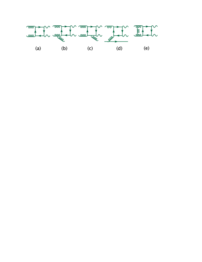
Figure 1: Representative parton scattering subprocesses for diphoton production in gluon-gluon scattering.

II Notation and Subprocesses

II.1 Notation

We consider the scattering process $h_{1}(P_{1})+h_{2}(P_{2})\rightarrow\gamma(P_{3})+\gamma(P_{4})+X$, where $h_{1}$ and $h_{2}$ are the initial-state hadrons. In terms of the center-of-mass collision energy $\sqrt{S}$, the $\gamma\gamma$ invariant mass $Q$, the $\gamma\gamma$ transverse momentum $Q_{T}$, and the $\gamma\gamma$ rapidity $y$, the momenta $P_{1}^{\mu}$ and $P_{2}^{\mu}$ of the initial hadrons and $q^{\mu}\equiv P_{3}^{\mu}+P_{4}^{\mu}$ of the pair are expressed in the laboratory frame as

$$P_{1}^{\mu} = \frac{\sqrt{S}}{2}\left\{1,0,0,1\right\};$$ (1)

$$P_{2}^{\mu} = \frac{\sqrt{S}}{2}\left\{1,0,0,-1\right\};$$ (2)

$$q^{\mu} = \left\{\sqrt{Q^{2}+Q_{T}^{2}}\cosh y,Q_{T},0,\sqrt{Q^{2}+Q_{T}^{2}}\sinh y\right\}.$$ (3)

The light-cone momentum fractions for the boosted $2\rightarrow 2$ scattering system are

$$x_{1,2}\equiv\frac{2(P_{2,1}\cdot q)}{S}=\frac{\sqrt{Q^{2}+Q_{T}^{2}}e^{\pm y}}{\sqrt{S}}.$$ (4)

Decay of the $\gamma\gamma$ pairs is described in the hadronic Collins-Soper frame Collins and Soper (1977). The Collins-Soper frame is a rest frame of the $\gamma\gamma$ pair (with $q^{\mu}=\left\{Q,0,0,0\right\}$ in this frame), chosen so that (a) the momenta $\vec{P}_{1}$ and $\vec{P}_{2}$ of the initial hadrons lie in the $Oxz$ plane (with zero azimuthal angle), and (b) the $z$ axis bisects the angle between $\vec{P}_{1}$ and $-\vec{P}_{2}$. The photon momenta are antiparallel in the Collins-Soper frame:

$$P_{3}^{\mu} = \frac{Q}{2}\left\{0,\sin\theta_{*}\cos\varphi_{*},\sin\theta_{*}\sin\varphi_{*},\cos\theta_{*}\right\},$$ (5)

$$P_{4}^{\mu} = \frac{Q}{2}\left\{0,-\sin\theta_{*}\cos\varphi_{*},-\sin\theta_{*}\sin\varphi_{*},-\cos\theta_{*}\right\},$$ (6)

where $\theta_{*}$ and $\varphi_{*}$ are the photon’s polar and azimuthal angles. Our aim is to derive resummed predictions for the fully differential $\gamma\gamma$ cross section $d\sigma/(dQ^{2}dydQ_{T}^{2}d\Omega_{*}),$ where $d\Omega_{*}=d\cos\theta_{*}d\varphi_{*}$ is a solid angle element around the direction of $\vec{P}_{3}$ in the Collins-Soper frame of reference defined in Eq. (5). The parton momenta and helicities are denoted by lowercase $p_{i}$ and $\lambda_{i}$.

II.2 Scattering contributions

We concentrate on direct production of isolated photons in hard QCD scattering, the dominant production process at hadron colliders. A number of hard-scattering contributions to the processes $q\bar{q}+qg\rightarrow\gamma\gamma,$ as well as photon production via fragmentation, have been studied in the past Aurenche et al. (1985); Bailey et al. (1992); Binoth et al. (2000). Our numerical calculations include the lowest-order process $q\bar{q}\rightarrow\gamma\gamma$ of order ${\cal O}(\alpha^{2})$ and contributions from $q\bar{q}\rightarrow\gamma\gamma g$ and $q^{\!\!\!\!\!{}^{(-)}}g\rightarrow\gamma\gamma q^{\!\!\!\!\!{}^{(-)}}$ of order ${\cal O}(\alpha^{2}\alpha_{s}),$ where $\alpha(\mu)=e^{2}/4\pi$ and $\alpha_{s}(\mu)=g^{2}/4\pi$ are the running QED and QCD coupling strengths.

Glue-glue scattering is the next leading direct production channel, with the full set of NLO contributions shown in Fig. 1. Production of $\gamma\gamma$ pairs via a box diagram in $gg$ scattering as in Fig. 1(a) Berger et al. (1984) is suppressed by two powers of $\alpha_{s}$ compared to the lowest-order $q\bar{q}\rightarrow\gamma\gamma$ contribution, but is enhanced by a product of two large gluon PDF’s if typical momentum fractions $x$ are small. The main ${\mathcal{O}}(\alpha^{2}\alpha_{s}^{3})$, or NLO, corrections, include one-loop $gg\rightarrow\gamma\gamma g$ diagrams (b) and (c) derived in Balazs et al. (2000); de Florian and Kunszt (1999), as well as 4-leg two-loop diagrams (e) computed in Bern et al. (2001). The real and virtual diagrams are combined in Ref. Bern et al. (2002) to obtain the full NLO contribution from $gg$ scattering. In this study we also include subleading NLO contributions from the process (d), $gq_{S}\rightarrow\gamma\gamma q_{S}$ via the quark loop, where $q_{S}=\sum_{i=u,d,s,...}(q_{i}+\bar{q}_{i})$ denotes the flavor-singlet combination of quark scattering channels. The $gq_{S}\rightarrow\gamma\gamma q_{S}$ helicity amplitude is derived from the one-loop $q\bar{q}ggg$ amplitude Bern et al. (1995) and explicitly presented in Appendix A. As a cross check, we verified that this amplitude correctly reproduces the known collinear limits. Our result does not confirm an expression for this amplitude available in the literature Yasui (2002), which does not satisfy these limits. When evaluated in our resummation calculation under typical event selection conditions, $gg+gq_{S}$ scattering contributes about 20% and 10% of the total rate at the LHC and the Tevatron, respectively, but this fraction can be larger in specific regions of phase space.

III Theoretical Presentation

III.1 Small-$Q_{T}$ asymptotics of the next-to-leading order cross section

When the transverse momentum $Q_{T}$ of the diphoton approaches zero, the NLO production cross section $d\sigma/(dQ^{2}dy\,dQ_{T}^{2}d\Omega_{*})$, or briefly $P(Q,Q_{T},y,\Omega_{*}),$ is dominated by $\gamma\gamma$ recoil against soft and collinear QCD radiation. In this subsection we concentrate on the effects of initial-state QCD radiation and derive the leading small-$Q_{T}$ part of the NLO differential cross section, called the asymptotic term $A(Q,Q_{T},y,\Omega_{*})$.

The ${\mathcal{O}}(\alpha_{s})$ asymptotic cross section valid at $Q_{T}^{2}\ll Q^{2}$ consists of a few generalized functions that are integrable on an interval $0\leq Q_{T}\leq P_{T}$, with $P_{T}$ being a finite value of transverse momentum:

$$A(Q,Q_{T},y,\Omega_{*})=F_{\delta}(Q,y,\Omega_{*})\delta(\vec{Q}_{T})$$ (7)

$$+ F_{1}(Q,y,\Omega_{*})\left[\frac{1}{Q_{T}^{2}}\ln\frac{Q^{2}}{Q_{T}^{2}}\right]_{+}+F_{0}(Q,y,\Omega_{*})\left[\frac{1}{Q_{T}^{2}}\right]_{+}+\dots.$$

The “$+$” prescription $\left[f(Q_{T})\right]_{+}$ is defined for a function $f(Q_{T})$ and a smooth function $g(Q_{T})$ as

$$\int_{0}^{P_{T}^{2}}dQ_{T}^{2}\left[f(Q_{T})\right]_{+}g(Q_{T}) \equiv \int_{0}^{P_{T}^{2}}dQ_{T}^{2}f(Q_{T})\left(g(Q_{T})-g(0)\right);$$ (8)

$$\left[f(Q_{T})\right]_{+}=f(Q_{T}) Q_{T}\neq 0.$$ for (9)

Subleading terms proportional to $\left(Q/Q_{T}\right)^{p}$ with $p\leq 1$ are neglected in Eq. (7). Its form is influenced by spin correlations between the initial-state partons and final-state photons. As a consequence of these spin correlations, the functions $F_{\delta},$ $F_{0}$, and $F_{1}$ depend on the direction of the final-state photons in the Collins-Soper frame (the polar angle $\theta_{*}$ and sometimes the azimuthal angle $\varphi_{*}$).

The spin dependence of the small-$Q_{T}$ cross section in the $gg\rightarrow\gamma\gamma g$ and $gq_{S}\rightarrow\gamma\gamma q_{S}$ channels is complex. The Born-level process $g(p_{1},\lambda_{1})+g(p_{2},\lambda_{2})\rightarrow\gamma(p_{3},\lambda_{3})+\gamma(p_{4},\lambda_{4})$ is described by 16 non-zero helicity amplitudes ${\mathcal{M}}_{4}(p_{1},\lambda_{1};p_{2},\lambda_{2};p_{3},\lambda_{3};p_{4},\lambda_{4})\equiv{\mathcal{M}}_{4}(\lambda_{1},\lambda_{2},\lambda_{3},\lambda_{4})$ for quark-box diagrams of the type shown in Fig. 1(a). The normalization of ${\mathcal{M}}_{4}(\lambda_{1},\lambda_{2},\lambda_{3},\lambda_{4})$ is chosen so that the unpolarized Born $gg\rightarrow\gamma\gamma$ cross section reads as

$$\left.\frac{d\sigma_{gg}}{dQ^{2}dy\,dQ_{T}^{2}d\Omega_{*}}\right|_{Born}=\delta(\vec{Q}_{T})\frac{\Sigma_{g}(\theta_{*})}{S}f_{g/h_{1}}(x_{1},\mu_{F})f_{g/h_{2}}(x_{2},\mu_{F}),$$ (10)

where

$$\Sigma_{g}(\theta_{*})\equiv\sigma_{g}^{(0)}L_{g}(\theta_{*}),$$ (11)

with

$$\sigma_{g}^{(0)}=\frac{\alpha^{2}(Q)\alpha_{s}^{2}(Q)}{32\pi Q^{2}(N_{c}^{2}-1)}\left(\sum_{i}e_{i}^{2}\right)^{2},$$ (12)

and

$$L_{g}(\theta_{*})\equiv\sum_{\lambda_{1},\lambda_{2},\lambda_{3},\lambda_{4}=\pm 1}\left|{\mathcal{M}}_{4}(\lambda_{1},\lambda_{2},\lambda_{3},\lambda_{4})\right|^{2}.$$ (13)

In these equations, $N_{c}=3$ is the number of QCD colors, $e_{i}$ is the fractional electric charge (in units of the positron charge $e$) of the quark $i$ circulating in the loop, and $f_{g/h}(x,\mu_{F})$ is the gluon PDF evaluated at a factorization scale $\mu_{F}$. The right-hand side of Eq. (13) includes summation over gluon and photon helicities $\lambda_{i}$, with $i=1,...,4$.

At NLO, the small-$Q_{T}$ cross section is proportional to the angular function $\Sigma_{g}(\theta_{*})$ (the same as in the Born cross section), and another function

$$\Sigma_{g}^{\prime}(\theta_{*},\varphi_{*}) = \sigma_{g}^{(0)}\sum_{\lambda_{1},\lambda_{2},\lambda_{3},\lambda_{4}=\pm 1}{\mathcal{M}}_{4}^{*}(\lambda_{1},\lambda_{2},\lambda_{3},\lambda_{4}){\mathcal{M}}_{4}(-\lambda_{1},\lambda_{2},\lambda_{3},\lambda_{4})$$ (14)

$$\equiv \sigma_{g}^{(0)}L_{g}^{\prime}(\theta_{*})\cos 2\varphi_{*}.$$

The function $\Sigma_{g}^{\prime}(\theta_{*},\varphi_{*})$ is obtained by spin-averaging the product of the amplitude ${\mathcal{M}}_{4}(\lambda_{1},\lambda_{2},\lambda_{3},\lambda_{4}),$ and the complex-conjugate amplitude ${\mathcal{M}}_{4}^{*}(-\lambda_{1},\lambda_{2},\lambda_{3},\lambda_{4})$ evaluated with the reverse sign of the helicity $\lambda_{1}$. The sign flip for $\lambda_{1}$ results in dependence of $\Sigma_{g}^{\prime}(\theta_{*},\varphi_{*})$ on $\cos 2\varphi_{*}$. The $\theta_{*}$ dependence of $\Sigma_{g}^{\prime}(\theta_{*},\varphi_{*})$ enters through the function

$$L_{g}^{\prime}(\theta_{*}) = -4\mbox{{Re}}\left(M_{1,1,-1,-1}^{(1)}+M_{1,-1,1,-1}^{(1)}+M_{-1,1,1,-1}^{(1)}+1\right),$$ (15)

presented in terms of reduced amplitudes $M_{\lambda_{1},\lambda_{2},\lambda_{3},\lambda_{4}}^{(1)}$ in the notation of Ref. Bern et al. (2001). For comparison, the functions $L_{g}(\theta_{*})$ and $L_{g}^{\prime}(\theta_{*})$ are plotted versus $(1+\cos\theta_{*})/2$ in Fig. 2.

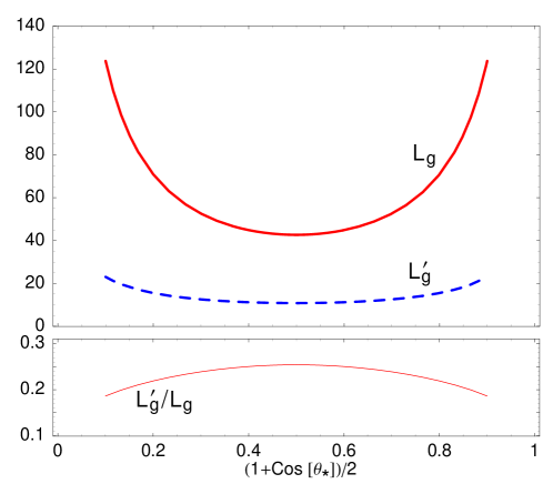
Figure 2: The functions $L_{g}(\theta_{*})$ and $L_{g}^{\prime}(\theta_{*})$ arising in the $gg\rightarrow\gamma\gamma$ asymptotic cross section (16) and their ratio.

The NLO asymptotic term in the sum of the contributions from the $gg\rightarrow\gamma\gamma$ and $gq_{S}\rightarrow\gamma\gamma$ channels (denoted as $gg+gq_{S}$ channel) is

$$A(Q,Q_{T},y,\Omega_{*}) = \frac{1}{S}\Biggl{\{}\Sigma_{g}(\theta_{*})\left[\delta(\vec{Q}_{T})F_{g,\delta}(Q,y,\theta_{*})+F_{g,+}(Q,y,Q_{T})\right]$$ (16)

$$\hskip 12.0pt+\Sigma_{g}^{\prime}(\theta_{*},\varphi_{*})F_{g,+}^{\prime}(Q,y,Q_{T})\Biggr{\}}.$$

Here

$$F_{g,\delta}\equiv f_{g/h_{1}}(x_{1},\mu_{F})f_{g/h_{2}}(x_{2},\mu_{F})\left(1+2\frac{\alpha_{s}}{\pi}h_{g}^{(1)}(\theta_{*})\right)$$ (17)

$$+ \frac{\alpha_{s}}{\pi}\Biggl{\{}\left(\left[{\mathcal{C}}_{g/a}^{(1,c)}\otimes f_{a/h_{1}}\right](x_{1},\mu_{F})-\left[P_{g/a}\otimes f_{a/h_{1}}\right](x_{1},\mu_{F})\,\ln\frac{\mu_{F}}{Q}\right)\,f_{g/h_{2}}(x_{2},\mu_{F})$$

$$\hskip 27.0pt+f_{g/h_{1}}(x_{1},\mu_{F})\left(\left[{\mathcal{C}}_{g/a}^{(1,c)}\otimes f_{a/h_{2}}\right](x_{2},\mu_{F})-\left[P_{g/a}\otimes f_{a/h_{2}}\right](x_{2},\mu_{F})\,\ln\frac{\mu_{F}}{Q}\right)\Biggr{\}};$$

$$F_{g,+} = \frac{1}{2\pi}\frac{\alpha_{s}}{\pi}\Biggl{\{}f_{g/h_{1}}(x_{1},\mu_{F})f_{g/h_{2}}(x_{2},\mu_{F})\left({\mathcal{A}}_{g}^{(1,c)}\left[\frac{1}{Q_{T}^{2}}\ln\frac{Q^{2}}{Q_{T}^{2}}\right]_{+}+{\mathcal{{\mathcal{B}}}}_{g}^{(1,c)}\left[\frac{1}{Q_{T}^{2}}\right]_{+}\right)$$ (18)

$$+ \left[\frac{1}{Q_{T}^{2}}\right]_{+}\Bigl{(}\left[P_{g/a}\otimes f_{a/h_{1}}\right](x_{1},\mu_{F})\,f_{g/h_{2}}(x_{2},\mu_{F})$$

$$\hskip 47.0pt+f_{g/h_{1}}(x_{1},\mu_{F})\left[P_{g/a}\otimes f_{a/h_{2}}\right](x_{2},\mu_{F})\Bigr{)}\Biggr{\}};$$

and

$$F_{g,+}^{\prime} = \frac{1}{2\pi}\frac{\alpha_{s}}{\pi}\left[\frac{1}{Q_{T}^{2}}\right]_{+}\Bigl{(}\left[P_{g/g}^{\prime}\otimes f_{g/h_{1}}\right](x_{1},\mu_{F})\,f_{g/h_{2}}(x_{2},\mu_{F})$$ (19)

$$\hskip 77.0pt+f_{g/h_{1}}(x_{1},\mu_{F})\left[P_{g/g}^{\prime}\otimes f_{g/h_{2}}\right](x_{2},\mu_{F})\Bigr{)}.$$

The ${\cal O}(\alpha_{s}/\pi)$ coefficients ${\mathcal{A}}_{g}^{(1,c)}$, ${\mathcal{B}}_{g}^{(1,c)}$ and functions ${\mathcal{C}}_{g/a}^{(1,c)}(x,b)$, $h_{g}^{(1)}(\theta_{*})$ are defined and listed explicitly in Ref. Balazs et al. (2007). The function $h_{g}^{(1)}(\theta_{*})$ denotes an ${\cal O}(\alpha_{s}/\pi)$ correction to the hard-scattering contribution ${\cal H}$ in the resummed cross section, cf. Sec. III.4. The convolutions $\left[P_{g/a}\otimes f_{a/h}\right]$ and $\left[{\mathcal{C}}_{g/a}^{(1,c)}\otimes f_{a/h}\right]$, defined for two functions $f(x,\mu_{F})$ and $g(x,\mu_{F})$ as

$$[f\otimes g](x,\mu_{F})\equiv\int_{x}^{1}\frac{d\xi}{\xi}f(\xi,\mu_{F})g(\frac{x}{\xi},\mu_{F}),$$

are summed over the intermediate parton’s flavors $a=g,\,q_{S}$ (gluon and the flavor-singlet combination of quark-scattering channels). In addition to the conventional splitting functions $P_{g/g}(x)$ and $P_{g/q_{S}}(x)$ arising in $F_{g,+}$, a new splitting function

$$P_{g/g}^{\prime}(x)=2C_{A}(1-x)/x,$$ (20)

where $C_{A}=N_{c}=3,$ enters the $\varphi_{*}$-dependent part of the asymptotic cross section through $F_{g,+}^{\prime}.$

For completeness, the small-$Q_{T}$ asymptotic form Eq. (16) for the $gg+gq_{S}$ channels is derived in Appendix B. The existence of the $\varphi_{*}-$dependent singular contribution proportional to $\Sigma_{g}^{\prime}(\theta_{*},\varphi_{*})$ is established by examining the factorization of the $2\rightarrow 3$ cross section in the limit of a collinear gluon emission. It follows directly from factorization rules for helicity amplitudes Bern et al. (1993, 1994a, 1994b, 1995, 1998, 1999); Kosower and Uwer (1999), as well as from the dipole factorization formalism Catani and Seymour (1997).

In contrast, the NLO quark-antiquark contribution $q\bar{q}\rightarrow\gamma\gamma$ does not include a spin-flip contribution, as a result of the simple structure of the Born contribution in $q\bar{q}$ scattering (see also Sec. III.3).

III.2 Resummation

To predict the shape of $d\sigma/dQ_{T}$ distributions, we perform an all-orders summation of singularities $\delta(\vec{Q}_{T})$ and $\left[Q_{T}^{-2}\ln^{p}\left(Q^{2}/Q_{T}^{2}\right)\right]_{+}$ in the asymptotic cross section, which coincides with the perturbative expansion of the resummed small-$Q_{T}$ cross section obtained within the Collins-Soper-Sterman formalism Collins and Soper (1981); Collins and Soper (1982a); Collins et al. (1985). In this formalism, we write the fully differential cross section as

$$\frac{d\sigma(h_{1}h_{2}\rightarrow\gamma\gamma)}{dQ\,dQ_{T}^{2}\,dy\,d\Omega_{*}}=W(Q,Q_{T},y,\Omega_{*})+Y(Q,Q_{T},y,\Omega_{*}).$$ (21)

The term $W$ contains large logarithmic contributions of the form $\ln^{p}(Q/Q_{T})$ from initial-state radiation, while $Y$ is free of these logs and calculated using collinear QCD factorization (cf. the end of Sec. III.4).

The function $W$ may be expressed as a Fourier-Bessel transform of a function $\widetilde{W}(Q,b,y,\Omega_{*})$ in the impact parameter (${\vec{b}}$) space,

$$W(Q,Q_{T},y,\Omega_{*})=\int\frac{d\vec{b}}{(2\pi)^{2}}e^{i\vec{Q}_{T}\cdot\vec{b}}\widetilde{W}(Q,b,y,\Omega_{*}).$$ (22)

The generic form of $\widetilde{W}(Q,b,y,\Omega_{*})$ in the $q\bar{q}+qg\rightarrow\gamma\gamma$ and $gg+gq_{S}\rightarrow\gamma\gamma$ channels can be determined by solving evolution equations for the gauge- and renormalization-group invariance of $\widetilde{W}(Q,b,y,\Omega_{*})$:

$$\widetilde{W}(Q,b,y,\Omega_{*}) = \sum_{a}\sum_{\lambda_{1},\lambda_{1}^{\prime},\lambda_{2},\lambda_{2}^{\prime},\lambda_{3},\lambda_{4}}{\mathcal{H}}_{a}^{\lambda_{1}\lambda_{2}\lambda_{3}\lambda_{4}}(Q,\Omega_{*})\left({\mathcal{H}}_{a}^{\lambda_{1}^{\prime}\lambda_{2}^{\prime}\lambda_{3}\lambda_{4}}(Q,\Omega_{*})\right)^{*}$$ (23)

$$\hskip 84.0pt\times{\mathcal{P}}_{a/h_{1}}^{\lambda_{1}\lambda_{1}^{\prime}}(x_{1},\vec{b})\,{\mathcal{P}}_{\bar{a}/h_{2}}^{\lambda_{2}\lambda_{2}^{\prime}}(x_{2},\vec{b})\,e^{-{\mathcal{S}}_{a}(Q,b)}.$$

It is composed of the hard-scattering function ${\mathcal{H}}_{a}^{\lambda_{1}\lambda_{2}\lambda_{3}\lambda_{4}}(Q,\Omega_{*})$ and its complex conjugate, $\left({\mathcal{H}}_{a}^{\lambda_{1}^{\prime}\lambda_{2}^{\prime}\lambda_{3}\lambda_{4}}(Q,\Omega_{*})\right)^{*};$ the Sudakov exponential $\exp\left(-{\mathcal{S}}_{a}(Q,b)\right)$; and parton distribution matrices ${\mathcal{P}}_{a/h_{i}}^{\lambda_{i}\lambda_{i}^{\prime}}(x_{i},\vec{b})$.

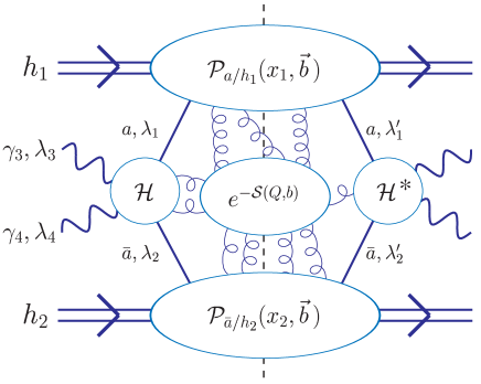
Figure 3: The structure of the resummed form factor $\widetilde{W}(Q,b,y,\Omega_{*})$.

The multiplicative structure of Eq. (23) reflects the topology of the dominant cut diagrams in the small-$Q_{T}$ cross sections shown in Fig. 3. The function ${\mathcal{H}}_{a}^{\lambda_{1}\lambda_{2}\lambda_{3}\lambda_{4}}$ describes the hard $2\rightarrow 2$ scattering subprocess $a(p_{1},\lambda_{1})+\bar{a}(p_{2},\lambda_{2})\rightarrow\gamma(p_{3},\lambda_{3})+\gamma(p_{4},\lambda_{4})$, with $a=u,\bar{u},d,\bar{d},...$ in $q\bar{q}\rightarrow\gamma\gamma$, and $a=\bar{a}=g$ in $gg\rightarrow\gamma\gamma$. All momenta in ${\mathcal{H}}$ have virtualities of order $Q^{2}.$ For now, we consider the leading contribution to ${\mathcal{H}}_{a}^{\lambda_{1}\lambda_{2}\lambda_{3}\lambda_{4}},$ which reads as ${\mathcal{H}}_{a}^{\lambda_{1}\lambda_{2}\lambda_{3}\lambda_{4}}=\sqrt{\sigma_{a}^{(0)}}{\mathcal{M}}_{4}(\lambda_{1},\lambda_{2},\lambda_{3},\lambda_{4}),$ where the Born helicity amplitude ${\mathcal{M}}_{4}(\lambda_{1},\lambda_{2},\lambda_{3},\lambda_{4})$ and overall constant normalization $\sigma_{a}^{(0)}$ are introduced in Sec. III.1. Sometimes ${\mathcal{H}}_{a}^{\lambda_{1}\lambda_{2}\lambda_{3}\lambda_{4}}$ also includes finite parts of higher-order $2\rightarrow 2$ virtual corrections, as discussed in Sec. III.4.

Similarly, $\left({\mathcal{H}}_{a}^{\lambda_{1}^{\prime}\lambda_{2}^{\prime}\lambda_{3}\lambda_{4}}(Q,\Omega_{*})\right)^{*}$ arises from the complex-conjugate amplitude ${\mathcal{M}}_{4}^{*}(\lambda_{1},\lambda_{2},\lambda_{3},\lambda_{4})$ and possible loop corrections to it. The helicities $\lambda_{1}^{\prime}$ and $\lambda_{2}^{\prime}$ in $\left({\mathcal{H}}_{a}^{\lambda_{1}^{\prime}\lambda_{2}^{\prime}\lambda_{3}\lambda_{4}}\right)^{*}$ need not coincide with $\lambda_{1}$ and $\lambda_{2}$ in ${\mathcal{H}}_{a}^{\lambda_{1}\lambda_{2}\lambda_{3}\lambda_{4}}$ . The right-hand side of Eq. (23) is summed over flavors $a$ and helicities $\lambda_{k},\lambda_{k}^{\prime}$ of the partons entering ${\mathcal{H}}{\mathcal{{H}^{*}}}$, as well as over helicities $\lambda_{3}$ and $\lambda_{4}$ of the final-state photons.

The Sudakov exponent

$${\mathcal{S}}_{a}(Q,b)=\int_{C_{1}^{2}/b^{2}}^{C_{2}Q^{2}}\frac{d\bar{\mu}^{2}}{\bar{\mu}^{2}}\left[{\mathcal{A}}_{a}\left(C_{1},\bar{\mu}\right)\ln\left(\frac{C_{2}^{2}Q^{2}}{\bar{\mu}^{2}}\right)+{\mathcal{B}}_{a}\left(C_{1},C_{2},\bar{\mu}\right)\right]$$ (24)

resums contributions from the initial-state soft and soft-collinear gluon emission (indicated by gluon lines connecting $e^{-{\cal S}}$ to ${\cal H}$, ${\cal H}^{*},$ and ${\cal P}_{a/h}(x,\vec{b})$ in Fig. 3). Here $C_{1}$ and $C_{2}$ are constants of order unity. The functions ${\mathcal{A}}_{a}\left(C_{1},\bar{\mu}\right)$ and ${\mathcal{B}}_{a}\left(C_{1},C_{2},\bar{\mu}\right)$ can be evaluated in perturbation theory at large scales $\bar{\mu}^{2}\gg\Lambda_{QCD}^{2}$, hence for large $Q$ and small $b$.

The collinear emissions are described by parton distribution matrices ${\mathcal{P}}_{a/h}^{\lambda\lambda^{\prime}}(x,\vec{b})$, where $\lambda$ and $\lambda^{\prime}$ denote the helicity state of the intermediate parton $a$ to the left and right of the unitarity cut in Fig. 3. The matrix ${\mathcal{P}}_{a/h}^{\lambda\lambda^{\prime}}(x,\vec{b})$ is derived from a matrix element of the light-cone correlator Ralston and Soper (1979); Soper (1977, 1979); Ali and Hoodbhoy (1993); Bashinsky and Jaffe (1998) for finding parton $a$ inside the parent hadron $h$.

It is convenient to introduce sums of diagonal and off-diagonal entries of the helicity matrix ${\mathcal{P}}_{a/h}^{\lambda\lambda^{\prime}}(x,\vec{b})$,

$${\mathcal{P}}_{a/h}(x,\vec{b})=\sum_{\lambda}{\mathcal{P}}_{a/h}^{\lambda\lambda}(x,\vec{b}),$$ (25)

and

$${\mathcal{P}}_{a/h}^{\prime}(x,\vec{b})=\sum_{\lambda}{\mathcal{P}}_{a/h}^{\lambda,-\lambda}(x,\vec{b}).$$ (26)

In this notation, Eq. (23) can be rewritten as

$$\widetilde{W}(Q,b,y,\Omega_{*}) = \frac{1}{S}e^{-{\mathcal{S}}_{a}(Q,b)}\sum_{a}\Biggl{\{}\Sigma_{a}(\theta_{*}){\mathcal{P}}_{a/h_{1}}(x_{1},\vec{b})\,{\mathcal{P}}_{\bar{a}/h_{2}}(x_{2},\vec{b})+$$

$$+ \Sigma_{a}^{\prime}(\theta_{*},\varphi_{*})\left[{\mathcal{P}}_{a/h_{1}}^{\prime}(x_{1},\vec{b})\,{\mathcal{P}}_{\bar{a}/h_{2}}(x_{2},\vec{b})+{\mathcal{P}}_{a/h_{1}}(x_{1},\vec{b})\,{\mathcal{P}}_{\bar{a}/h_{2}}^{\prime}(x_{2},\vec{b})\right]$$

$$+ \Sigma_{a}^{\prime\prime}(\theta_{*},\varphi_{*}){\mathcal{P}}_{a/h_{1}}^{\prime}(x_{1},\vec{b})\,{\mathcal{P}}_{\bar{a}/h_{2}}^{\prime}(x_{2},\vec{b})\Biggr{\}},$$

where

$$\Sigma_{a}(\theta_{*}) \equiv \sum_{\lambda_{1},\lambda_{2},\lambda_{3},\lambda_{4}}\left|{\mathcal{H}}_{a}^{\lambda_{1}\lambda_{2}\lambda_{3}\lambda_{4}}\right|^{2},$$ (28)

$$\Sigma_{a}^{\prime}(\theta_{*},\varphi_{*}) \equiv \sum_{\lambda_{1},\lambda_{2},\lambda_{3},\lambda_{4}}{\mathcal{H}}_{a}^{\lambda_{1}\lambda_{2}\lambda_{3}\lambda_{4}}\left({\mathcal{H}}_{a}^{-\lambda_{1}\lambda_{2}\lambda_{3}\lambda_{4}}\right)^{*},$$ (29)

and

$$\Sigma_{a}^{\prime\prime}(\theta_{*},\varphi_{*})\equiv\sum_{\lambda_{1},\lambda_{2},\lambda_{3},\lambda_{4}}{\mathcal{H}}_{a}^{\lambda_{1}\lambda_{2}\lambda_{3}\lambda_{4}}\left({\mathcal{H}}_{a}^{-\lambda_{1}-\lambda_{2}\lambda_{3}\lambda_{4}}\right)^{*}.$$ (30)

The unpolarized parton distribution ${\mathcal{P}}_{a/h}(x,\vec{b})$ coincides with the Fourier-Bessel transform of the unpolarized transverse-momentum-dependent (TMD) parton density ${\mathcal{P}}_{a/h}(x,\vec{k}_{T})$ Collins and Soper (1982b) for finding parton $a$ with light-cone momentum fraction $x$ and transverse momentum $\vec{k}_{T}$. At small $b,$ ${\mathcal{P}}_{a/h}(x,\vec{b})$ is reduced to a convolution of unpolarized $k_{T}-$integrated parton densities $f_{a/h}(x,\mu)$ and Wilson coefficient functions ${\mathcal{C}}_{a/a^{\prime}}(x,b;C/C_{2},\mu)$, evaluated at a factorization scale $\mu$ of order $1/b$:

$$\left.{\mathcal{P}}_{a/h}(x,\vec{b})\right|_{b^{2}\ll\Lambda_{QCD}^{-2}} = \sum_{a^{\prime}}\left[\int_{x}^{1}{\frac{d\xi}{\xi}}{\mathcal{C}}_{a/a^{\prime}}\left(\frac{x}{\xi},b;\frac{C_{1}}{C_{2}},\mu\right)f_{a^{\prime}/h}(\xi,\mu)\right].$$ (31)

Perturbative entries with $\lambda_{i}=\lambda_{i}^{\prime}$ reduce in total to the product of the unpolarized Born scattering probability and unpolarized resummed functions:

$$\left.\widetilde{W}(Q,b,y,\Omega_{*})\right|_{\lambda_{i}=\lambda_{i}^{\prime}} = \sum_{a}\frac{\Sigma_{a}(\theta_{*})}{S}e^{-{\mathcal{S}}_{a}(Q,b)}$$ (32)

$$\times \left[{\mathcal{C}}_{a/c_{1}}\otimes f_{c_{1}/h_{1}}\right](x_{1},b;\mu)\left[{\mathcal{C}}_{\bar{a}/c_{2}}\otimes f_{c_{2}/h_{2}}\right](x_{2},b;\mu).$$

The function $\Sigma_{g}(\theta_{*})$ is shown explicitly in Eq. (11).

III.3 Spin-flip term in gluon scattering

We concentrate in this subsection on the spin-flip distribution ${\mathcal{P}}_{g/h}^{\prime}(x,\vec{b})$ in gluon scattering. Its existence is warranted by basic symmetries of helicity- and transverse-momentum-dependent gluon distribution functions Mulders and Rodrigues (2001). This function, which describes interference of the amplitudes for nearly collinear gluons with opposite helicities, coincides with the function $H^{\perp}$ in Ref. Mulders and Rodrigues (2001) up to an overall factor. It contributes to unpolarized $Q_{T}$ distributions, because the hard-scattering product ${\mathcal{H}}_{g}^{\lambda_{1}\lambda_{2}\lambda_{3}\lambda_{4}}\left({\mathcal{H}}_{g}^{\lambda_{1}^{\prime}\lambda_{2}^{\prime}\lambda_{3}\lambda_{4}}\right)^{*}$ (with ${\mathcal{H}}_{g}^{\lambda_{1}\lambda_{2}\lambda_{3}\lambda_{4}}$ given by the quark box helicity amplitude in Fig. 1(a)) does not vanish for $\lambda_{1}=-\lambda_{1}^{\prime}$ or $\lambda_{2}=-\lambda_{2}^{\prime}$ . The presence of ${\mathcal{P}}_{g/h}^{\prime}(x,\vec{b})$ modifies dependence of the resummed cross section on the photon’s azimuthal angle $\varphi_{*}$ in the Collins-Soper frame. It vanishes after the integration over $\varphi_{*}$ is performed. In contrast, the helicity-diagonal part of $\widetilde{W}(Q,b,y,\Omega_{*})$ is independent of $\varphi_{*}$, cf. Eq. (32).

The gluon function ${\mathcal{P}}_{g/h}^{\prime}(x,\vec{b})$ is invariant under time reversal (i.e., is $T$-even) and acquires large contributions proportional to the unpolarized $T$-even PDF’s ${\mathcal{P}}_{g/h}(x,\vec{b})$ in the process of gluon radiation. These contributions require resummation via PDF evolution equations (similar to Dokshitzer-Gribov-Lipatov-Altarelli-Parisi equations Dokshitzer (1977); Gribov and Lipatov (1972a, b); Altarelli and Parisi (1977)) in order to predict the $\varphi_{*}$ dependence in the $gg$ channel.

At one loop, the mixing of spin-flip and unpolarized gluon PDF’s is driven by the convolution $\left[P_{g/g}^{\prime}\otimes f_{g/h}\right](x,\mu_{F})$ of the spin-flip splitting function $P_{g/g}^{\prime}(x)$ shown in Eq. (20) with the gluon PDF $f_{g/h}(x,\mu_{F})$. This convolution may be comparable to or exceed the analogous convolution $\left[P_{g/g}\otimes f_{g/h}\right](x,\mu_{F})$ of the unpolarized splitting function $P_{g/g}(x)$ for some $x$ and $\mu_{F}$ values, as shown in Fig. 4. As a result of the mixing, an additional $\varphi_{*}$-dependent term

$$\frac{\Sigma_{g}^{\prime}(\theta_{*},\varphi_{*})}{2\pi SQ_{T}^{2}}\frac{\alpha_{s}}{\pi}\Bigl{(}\left[P_{g/g}^{\prime}\otimes f_{g/h_{1}}\right](x_{1},\mu_{F})\,f_{g/h_{2}}(x_{2},\mu_{F})$$

$$\hskip 77.0pt+f_{g/h_{1}}(x_{1},\mu_{F})\left[P_{g/g}^{\prime}\otimes f_{g/h_{2}}\right](x_{2},\mu_{F})\Bigr{)}$$ (33)

arises in the unpolarized ${\mathcal{O}}(\alpha_{s})$ asymptotic piece, cf. Eq. (16). It is produced by the perturbative expansion of the entry proportional to $\Sigma_{g}^{\prime}(\theta_{*},\varphi_{*}){\mathcal{P}}_{g/h}(x_{i},\vec{b}){\mathcal{P}}_{g/h}^{\prime}(x_{j},\vec{b})$ in $\widetilde{W}(Q,b,y,\Omega_{*})$, with $\Sigma_{g}^{\prime}(\theta_{*},\varphi_{*})$ shown explicitly in Eqs. (14) and (15). Generally, the $\varphi_{*}$-dependent contribution is not small, even though it is suppressed comparatively to the unpolarized collinear contribution by the ratio $L_{g}^{\prime}(\theta_{*})/L_{g}(\theta_{*})$ shown in Fig. 2. For example, for $Q=100$ GeV at the LHC, its magnitude constitutes up to about a half of the collinear unpolarized asymptotic contribution,

$$\frac{\Sigma_{g}(\theta_{*})}{2\pi SQ_{T}^{2}}\frac{\alpha_{s}}{\pi}\Bigl{(}\left[P_{g/a}\otimes f_{a/h_{1}}\right](x_{1},\mu_{F})\,f_{g/h_{2}}(x_{2},\mu_{F})+f_{g/h_{1}}(x_{1},\mu_{F})\left[P_{g/a}\otimes f_{a/h_{2}}\right](x_{2},\mu_{F})\Bigr{)}.$$ (34)

The ${\mathcal{O}}(\alpha_{s})$ spin-flip $gg$ contribution does not mix with the $gq_{S}$ contribution.

In terms of the reduced matrix elements $M_{\lambda_{1}\lambda_{2}\lambda_{3}\lambda_{4}}^{(1)}$ defined in Bern et al. (2001), the double spin-flip hard vertex function $\Sigma_{g}^{\prime\prime}(\theta_{*},\varphi_{*})$ is

$$\Sigma_{g}^{\prime\prime}(\theta_{*},\varphi_{*}) = \sigma_{g}^{(0)}\left(L_{1g}^{\prime\prime}(\theta_{*})+L_{2g}^{\prime\prime}(\theta_{*})\cos\left(4\varphi_{*}\right)\right),$$ (35)

where

$$L_{1g}^{\prime\prime}(\theta_{*}) = 4{\mbox{Re}}\left(M_{1,1,-1,-1}^{(1)}+1\right),$$ (36)

and

$$L_{2g}^{\prime\prime}(\theta_{*}) = 4{\mbox{Re}}\left(M_{1,-1,-1,1}^{(1)}M_{1,-1,1,-1}^{(1)*}+1\right).$$ (37)

The perturbative expansion of the resummed entry proportional to $\Sigma_{g}^{\prime\prime}(\theta_{*},\varphi_{*}){P}_{g/h}^{\prime}(x_{i},\vec{b}){P}_{g/h}^{\prime}(x_{j},\vec{b})$ produces an NNLO term in the unpolarized $gg$ asymptotic piece,

$$\frac{\Sigma_{g}^{\prime\prime}(\theta_{*},\varphi_{*})}{2\pi SQ_{T}^{2}}\frac{\alpha_{s}^{2}}{\pi^{2}}\left[P_{g/g}^{\prime}\otimes f_{g/h_{1}}\right](x_{1},\mu_{F})\left[P_{g/g}^{\prime}\otimes f_{g/h_{2}}\right](x_{2},\mu_{F}).$$ (38)

The analogous quark function ${\mathcal{P}}_{q_{i}/h}^{\prime}(x,\vec{k}_{T})$ corresponds to the transversity distribution Tangerman and Mulders (1995) and is odd under time reversal ($T$-odd). It cannot be generated radiatively through conventional PDF evolution from the $T$-even unpolarized function ${\mathcal{P}}_{q_{i}/h}(x,\vec{k}_{T})$ and does not contribute to the NLO asymptotic term. We find $\Sigma_{q}^{\prime}=0,$ because the non-vanishing amplitudes ${\cal H}_{q}(q_{1}^{\lambda_{1}},\bar{q}_{2}^{\lambda_{2}},\gamma_{3}^{\lambda_{3}},\gamma_{4}^{\lambda_{4}})$ must have opposite helicities of the quark and antiquark ($\lambda_{1}=-\lambda_{2}$). Therefore, the functions ${\mathcal{P}}_{q_{i}/h}^{\prime}(x,\vec{b})$ contribute in pairs through the term proportional to $\Sigma_{q}^{\prime\prime}(\varphi_{*})=-(\alpha^{2}e_{i}^{4}\pi/(2N_{c}Q^{2}))\,\cos 2\varphi_{*}.$ These contributions are anticipated to be much smaller than the usual spin-average contribution and negligible at large $Q$, in analogy to unpolarized Drell-Yan production Henneman et al. (2002); Boer (2001).

In summary, the azimuthal angle ($\varphi_{*}$) dependence of photons in the $gg$ scattering channel is affected by large QCD contributions associated with interference between gluons of opposite helicities. These logarithmic corrections may arise at NLO through QCD radiation from conventional unpolarized PDF’s, a mechanism that is unique to gluon scattering. Other types of spin-interference contributions (not considered here) involve spin-flip PDF’s only. The soft and collinear logarithms associated with the spin-flip contributions must be resummed along the lines discussed in Ref. Idilbi et al. (2004). Given that $gg\rightarrow\gamma\gamma$ is the subleading production channel at the Tevatron and at the LHC, we henceforth neglect the gluon spin-flip contributions to the resummed $\widetilde{W}(Q,b,y,\Omega_{*})$, while subtracting the corresponding $\varphi_{*}$-dependent asymptotic contribution from the finite-order $2\rightarrow 3$ cross section. The nature of $gg$ spin-flip contributions can be explored by measuring the double-differential distribution in $\varphi_{*}$ and $Q_{T}$ at the LHC, a topic that is interesting also from the point of view of the Higgs boson search. Full resummation of the gluon spin-flip contributions may be needed in the future.

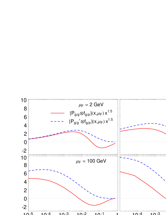
Figure 4: Comparison of $[P_{g/g}\otimes f_{g/p}](x,\mu_{F})$ and $[P_{g/g}^{\prime}\otimes f_{g/p}](x,\mu_{F})$ for the gluon PDF $f_{g/p}(x,\mu_{F})$ in the proton (multiplied by $x^{1.5}$ to better illustrate the small-$x$ region) at several values of the factorization scale $\mu_{F}.$

III.4 Complete expressions for resummed cross sections

In this Section, we review complete expressions for the unpolarized resummed cross sections, starting from the perturbative QCD approximation $\widetilde{W}_{pert}(Q,b,y,\Omega_{*})$ valid at small impact parameters $b^{2}\ll 1\mbox{ GeV}^{-2}$. For a hard-scattering function $\sum_{hel.}\left|{\mathcal{H}}(Q,\theta_{*})\right|^{2}\equiv\Sigma_{a}(\theta_{*})h_{a}^{2}(Q,\theta_{*}),$ the form factor $\widetilde{W}_{pert}(Q,b,y,\Omega_{*})$ is

$$\widetilde{W}_{pert}(Q,b,y,\theta_{*}) = \sum_{a}\frac{\Sigma_{a}(\theta_{*})}{S}h_{a}^{2}(Q,\theta_{*})e^{-{\mathcal{S}}_{a}(Q,b)}$$ (39)

$$\times \left[{\mathcal{C}}_{a/c_{1}}\otimes f_{c_{1}/h_{1}}\right](x_{1},b;\mu)\left[{\mathcal{C}}_{\bar{a}/c_{2}}\otimes f_{c_{2}/h_{2}}\right](x_{2},b;\mu).$$

The Sudakov function is defined in Eq. (24), and the function $h_{a}(Q,\theta_{*})$ collects radiative contributions to ${\mathcal{H}}(Q,\theta_{*})$ arising at NLO and beyond. We compute the functions $h_{a},$ ${\mathcal{A}}_{a}$, ${\mathcal{B}}_{a}$ and ${\mathcal{C}}_{a/c}$ up to orders $\alpha_{s},$ $\alpha_{s}^{3},$ $\alpha_{s}^{2},$ and $\alpha_{s},$ respectively. The ${\mathcal{A}}_{a}$, ${\mathcal{B}}_{a}$ and ${\mathcal{C}}_{a/c}$ coefficients are taken from Refs. Balazs et al. (1998); Nadolsky and Schmidt (2003); Yuan (1992); Vogt et al. (2004); de Florian and Grazzini (2000); Moch et al. (2004) and listed in a consistent notation in Ref. Balazs et al. (2007).

We use a procedure outlined in Ref. Balazs and Yuan (1997) to join the small-$Q_{T}$ resummed cross sections $W$ with the large-$Q_{T}$ NLO cross sections $P$. In Eq. (21), $Y\equiv P-A$ is the difference between the perturbative cross section $P$ and its small-$Q_{T}$ asymptotic expansion $A$, explicitly given in Eq. (16). For each value of $Q$ and $y$ of the $\gamma\gamma$ pair, $W+Y$ approaches $P$ from above and eventually becomes smaller than $P$ as $Q_{T}$ increases. We use $W+Y$ as our prediction at $Q_{T}$ values below this point of crossing and the finite-order cross section $P$ at $Q_{T}$ above the crossing point.

The final cross sections depend on several factorization scales: $C_{1}/b$, $C_{2}Q$, $\mu\equiv C_{3}/b$ in the $W$ term, and $\mu_{F}\equiv C_{4}Q$ in the $Y$ term. Here $C_{i}$ ($i=1,..4$) are dimensionless constants of order unity, chosen as $C_{2}=C_{4}=1$, $C_{1}=C_{3}=2e^{-\gamma_{E}}=1.123...$ by default. These choices simplify perturbative coefficients by eliminating scale-dependent logarithmic terms, cf. the appendix in Ref. Balazs et al. (2007). Dependence on the scale choice is studied in Section IV.

In the general formulation of CSS resummation presented in Collins and Soper (1981); Collins and Soper (1982a), one has the freedom to choose different “resummation schemes”, resulting effectively in variations in the form of $h_{a}(Q,\theta_{*})$. These differences are compensated, up to higher-order corrections, by adjustments in the functions ${\mathcal{B}}$ and ${\mathcal{C}}$.

In “the CSS resummation scheme” Collins et al. (1985), one chooses $h_{a}(Q,\theta_{*})=1,$ while including the virtual corrections to the $2\rightarrow 2$ scattering process in ${\mathcal{B}}$ and ${\mathcal{C}}.$ In this scheme, some ${\mathcal{B}}$ and ${\mathcal{C}}$ coefficients depend on the $2\rightarrow 2$ hard scattering process and also on $\theta_{*}$.

In an alternative prescription by Catani, de Florian and Grazzini Catani et al. (2001), “the CFG resummation scheme”, one keeps the $2\rightarrow 2$ virtual corrections within a single function $\left|{\mathcal{H}}(Q,\theta_{*})\right|^{2}.$ In this case, the ${\mathcal{B}}$ and ${\mathcal{C}}$ functions depend only on the initial state. Most of our numerical calculations are realized in the CSS resummation scheme, with a few made in the CFG scheme for comparison purposes.

In impact parameter ($b$) space used in the resummation procedure, we must integrate into the nonperturbative region of large $b$, cf. Eq. (22). Contributions from this region are known to be suppressed at high energies Berger and Qiu (2003), but some residual dependence may remain. In the $q\bar{q}+qg\rightarrow\gamma\gamma$ channel, our model for the nonperturbative contributions (denoted as KN1 Konychev and Nadolsky (2006)) is derived from the analysis of Drell-Yan pair and $Z$ boson production. The nonperturbative function in this model is dominated at large $Q$ by a soft contribution, which does not depend on the flavor of initial-state light quarks. This function is therefore expected to be applicable to the $q\bar{q}+qg\rightarrow\gamma\gamma$ process.

The nonperturbative function in the $gg+gq_{S}$ channel, which is yet to be measured directly, is approximated by the nonperturbative function for the $q\bar{q}+gq$ channel multiplied by the ratio $C_{A}/C_{F}=9/4$ of the color factors $C_{A}$ and $C_{F}$ for the leading soft contributions in the $gg$ and $q\bar{q}$ channels. This ansatz suggests stronger dependence of the $gg+gq_{S}$ channel on the nonperturbative input compared to the $q\bar{q}+qg$ channels. It leads to small differences from the prescription used in Refs. Balazs et al. (1998, 2000), where only the leading $\ln Q$ term of the nonperturbative function was rescaled. To examine the dependence of the resummed cross sections on the nonperturbative model, we evaluate some of them assuming an alternative (BLNY) parameterization of the nonperturbative function Landry et al. (2003).

IV Numerical Results

The analytical results of Sec. III are implemented in our computer codes Legacy and ResBos Ladinsky and Yuan (1994); Landry et al. (2003); Balazs and Yuan (1997); Balazs (1999). We use the same parameters as in the calculation of Ref. Balazs et al. (2006), and we concentrate on the region $Q_{T}<Q$ where our calculation is most reliable Balazs et al. (2006).

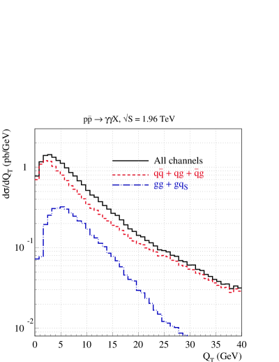
Figure 5: Parton flavor decomposition of the resummed transverse momentum distribution at the energy $\sqrt{S}=1.96$ TeV of the Tevatron Run-2. The total (solid), $q{\bar{q}}+qg$ (dashes), and $gg+gq_{S}$ (dash-dots) initial-state contributions are shown separately.

IV.1 Results for Run 2 at the Tevatron

In this section, we present our results for the Tevatron $p\bar{p}$ collider at $\sqrt{S}=1.96$ TeV. We make the same restrictions on the final-state photons as those used in the experimental measurement by the Collider Detector at Fermilab (CDF) collaboration Acosta et al. (2005): transverse momentum $p_{T}^{\gamma}>p_{T\,min}^{\gamma}=14\leavevmode\nobreak\ (13)$ GeV for the harder (softer) photon, and rapidity $|y^{\gamma}|<0.9$ for each photon. We impose photon isolation by requiring the hadronic transverse energy not to exceed $1$ GeV in the cone $\Delta R=0.4$ around each photon, as specified in the CDF publication. We also require the angular separation $\Delta R_{\gamma\gamma}$ between the photons to be larger than 0.3.

We focus in this paper on the role of the $gg$ contribution, referring to our other papers Balazs et al. (2006, 2007) for a more complete treatment.

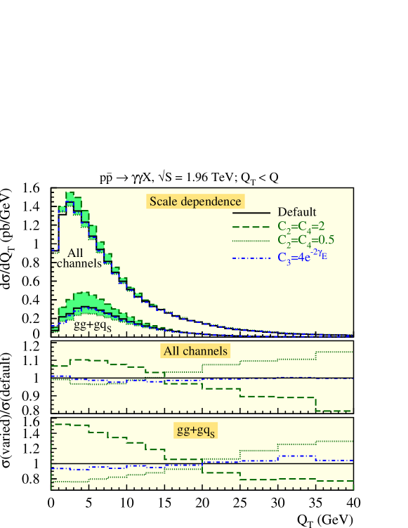
Figure 6: Scale dependence of the cross sections in $gg+gq_{S}$ and all scattering channels. The upper frame shows cross sections for the default choice of scales specified in Section III.4 (solid), as well as for varied scales $C_{2}=C_{4}=2$ (dashes), $C_{2}=C_{4}=0.5$ (dots), and $C_{3}=4e^{-2\gamma_{E}}$ (dot-dashes). The lower two frames show ratios of the cross sections computed for the varied factorization scales to the cross section for the default choice of the scales.

To illustrate the relative importance of the individual initial-state contributions in the final answer, we provide a parton flavor decomposition of our resummed transverse momentum distribution $d\sigma/dQ_{T}$ in Fig. 5. This distribution is integrated over all diphoton invariant masses $Q$, subject to the CDF cuts, and receives dominant contributions from the $Q_{T}<Q$ region. The $gg+gq_{S}$ contribution supplies about one-third of the total rate near $Q_{T}=5$ GeV. It falls steeply after $Q_{T}>20$ GeV, because the gluon PDF falls steeply with parton fractional momentum $x$.

Dependence of the resummed cross sections on the choice of factorization scales mentioned in Section III.4 is examined in Fig. 6. We pick a few characteristic combinations of alternative scales to probe the scale dependence associated with the resummed Sudakov function $e^{-{\cal S}}$, the $b$-dependent PDF’s ${\mathcal{P}}_{a/h}(x,\vec{b})\approx[{\mathcal{C}}_{a/c}\otimes f_{c/h}](x,b;\mu)$, and the regular $Y$ term. The small-$Q_{T}$ region is sensitive primarily to the scales $C_{1}/b,C_{2}\,Q,C_{3}/b$ in the resummed term $W$. The event rate at large $Q_{T}$ is controlled by the choice of the factorization scale $\mu_{F}\equiv C_{4}\,Q$ in the regular term $Y$.

At the relatively low values of $Q$ relevant for the Tevatron experiments, the scale dependence of the next-to-leading order $gg+gq_{S}$ cross section is still substantial, with variations being about $-20\%$ ($+50\%$) at $Q_{T}=5-10$ GeV, $\pm 10\%$ at $Q_{T}=10-20$ GeV, and $\pm 20\%$ at $Q_{T}=20-40$ GeV. Since the $Y$ term is the lowest-order approximation for $gg\rightarrow\gamma\gamma g$ at $Q_{T}\sim Q$, the scale dependence associated with the constant $C_{4}$ remains pronounced at large $Q_{T}$. The inclusive $gg+gq_{S}$ rate, integrated over $Q_{T}$, varies by $20-40\%$ almost independently of the $\gamma\gamma$ invariant mass $Q$. The large scale dependence of the NLO $gg+gq_{S}$ cross section reflects slow perturbative convergence in gluon gluon scattering, observed also in other similar processes, e.g., $gg\rightarrow\mbox{Higgs}$ via the top quark loop Harlander and Kilgore (2002); Anastasiou et al. (2004, 2005). For this reason, a NNLO calculation would be desirable to reduce the scale uncertainty in the $gg+gq_{S}$ channel.

On the other hand, the scale dependence of the cross section when all channels are combined is relatively mild, with variations not exceeding 10% at small $Q_{T}$ and 20% at large $Q_{T}$. Variations in the integrated inclusive rate for all channels combined are below 10% at $Q>30$ GeV.

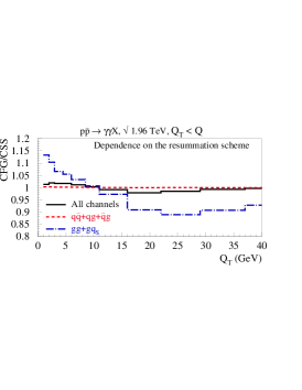
(a)

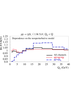
(b)

Figure 7: Ratios of resummed cross sections at the Tevatron Run-2 computed in (a) the Catani-de Florian-Grazzini (CFG) and Collins-Soper-Sterman (CSS) resummation schemes and (b) using the BLNY and KN1 nonperturbative models, as functions of the $\gamma\gamma$ transverse momentum $Q_{T}$. The ratios are shown in the $q\bar{q}+qg$ (dashed), $gg+gq_{S}$ (dot-dashed), and all (solid) scattering channels. A $Q_{T}<Q$ cut is imposed in this comparison.

Another aspect of scale dependence is associated with the assumed arrangement of logarithmic terms in the resummed $W$ term, i.e., the “resummation scheme” that is adopted. This dependence is yet another indicator of the size of higher-order corrections not included in the present analysis. Figure 7(a) shows ratios of the full resummed cross sections in the Catani-de Florian-Grazzini (CFG) and Collins-Soper-Sterman (CSS) resummation schemes, as described in Sec. III. The differences between these schemes stem from the different treatment of the NLO hard-vertex correction $h_{a}^{(1)}(\theta_{*})$. The magnitude of $h_{a}^{(1)}(\theta_{*})$ determines whether the channel is sensitive to the choice of the two resummation schemes. The magnitude of $h_{g}^{(1)}(\theta_{*})$ in the $gg+gq_{S}$ channel exceeds that of $h_{q}^{(1)}(\theta_{*})$ in the $q\bar{q}+qg$ channel by roughly an order of magnitude for most values of the $\theta_{*}$ angle Nadolsky and Schmidt (2003). Consequently, while the dependence on the resummation scheme is practically negligible in the dominant $q\bar{q}+qg$ channel (dashed line), it can reach 15% in the subleading $gg+gq_{S}$ channel (dot-dashed line). The $Q_{T}$ spectrum in $gg+gq_{S}$ channel is slightly softer in the CFG scheme up to the point of switching to the fixed-order cross section at $Q_{T}\approx 60$ GeV. The resummation scheme dependence in all channels (solid line) is less than 3-4%, reflecting mostly the scheme dependence in the $gg+gq_{S}$ channel.

To examine the sensitivity of the resummed predictions to long-distance nonperturbative dynamics in hadron-hadron scattering, we include in Fig. 7(b) a comparison with the resummed cross sections for an alternative choice of the nonperturbative model. As explained in Sec. III.4, our default calculation is performed in the recent KN1 model Konychev and Nadolsky (2006) for the nonperturbative part of the resummed form factor $\widetilde{W}(Q,b,y,\Omega_{*})$. Figure 7(b) shows ratios of the predictions for a different BLNY model Landry et al. (2003) and our default KN1 model in various initial-state scattering channels.

The difference is maximal at the lowest $Q_{T}$, as expected, and it is less than 5% for the total cross section. For the $q{\bar{q}}+qg$ and $gg+gq_{S}$ initial states the maximal difference is about 5% and 20%, respectively. The dependence on the nonperturbative function is stronger in the $gg+gq_{S}$ channel, where the BLNY/KN1 ratio in the $gg+gq_{S}$ channel reaches its maximum of 1.15 at $Q_{T}\approx 25$ GeV and slowly decreases toward 1, reached at the switching point at $Q_{T}\approx 60$ GeV. This behavior reflects our assumption of a larger magnitude of the nonperturbative function in the $gg+gq_{S}$ channel, which is rescaled in our model by $C_{A}/C_{F}=9/4$ compared to the nonperturbative function in the $q\bar{q}+qg$ channel. In summary, despite a few-percent uncertainty associated with the nonperturbative function in the $gg+gq_{S}$ process, the overall dependence of the Tevatron $\gamma\gamma$ cross section on the nonperturbative input can be neglected.

IV.2 Results for the LHC

To obtain predictions for $pp$ collisions at the LHC at $\sqrt{S}=14$ TeV, we employ the cuts on the individual photons used by the ATLAS collaboration in their simulations of Higgs boson decay, $h\rightarrow\gamma\gamma$ ATLAS Collaboration (1999). We require transverse momentum $p_{T}^{\gamma}>40\leavevmode\nobreak\ (25)$ GeV for the harder (softer) photon, and rapidity $|y^{\gamma}|<2.5$ for each photon. We impose the ATLAS isolation criteria, looser than for the Tevatron study, requiring less than 15 GeV of hadronic and extra electromagnetic transverse energy inside a $\Delta R=0.4$ cone around each photon. We also require the separation $\Delta R_{\gamma\gamma}$ between the two isolated photons to be above 0.4. The cuts optimized for the Higgs boson search may require adjustments in order to test perturbative QCD predictions in the full $\gamma\gamma$ invariant mass range accessible at the LHC.

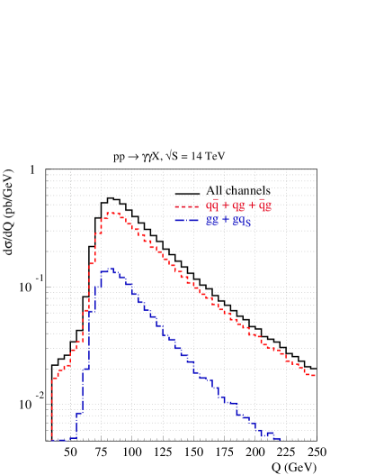
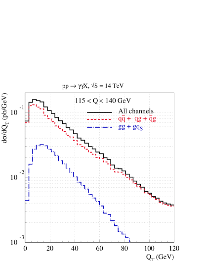
(a)                                                                  (b)

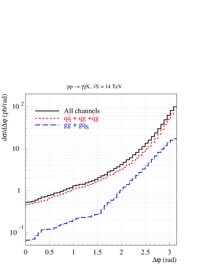
(c)

Figure 8: Resummed $d\sigma/dQ,$ $d\sigma/dQ_{T},$ and $d\sigma/d\Delta\varphi$ distributions of photon pairs at the LHC for ATLAS kinematic cuts.

Distributions in the invariant mass $Q$, transverse momentum $Q_{T}$, and azimuthal angle separation $\Delta\varphi\equiv\varphi_{\gamma_{1}}-\varphi_{\gamma_{2}}$ between the two photons in the laboratory frame are shown in Fig. 8. As before, we compare the magnitudes of the $q\bar{q}+qg$ and $gg+gq_{S}$ cross sections. The qualitative features are similar to those at the Tevatron, but the relative contribution of the various initial states changes at the LHC. The $gg+gq_{S}$ initial state contributes about 25% of the total rate at $Q\sim 80$ GeV where the mass distribution peaks, but the $gg+gq_{S}$ rate falls faster than $q\bar{q}+qg$ with increasing invariant mass.

In the invariant mass range relevant for the Higgs boson search, $115<Q<140$ GeV, the transverse momentum distribution in Fig. 8(b) shows that the $gg+gq_{S}$ initial state accounts for about 25% of the rate at low $Q_{T}$. At high transverse momentum, on the other hand, the other channels dominate. The relative size of the $gg+gq_{S}$ contribution drops as the invariant mass or the transverse momentum of the photon pair grows. The $gg+gq_{S}$ contribution falls more steeply with $Q_{T}$ for larger masses of the diphoton. These features are attributable to the steeply falling gluon distribution as a function of increasing momentum fraction $x$.

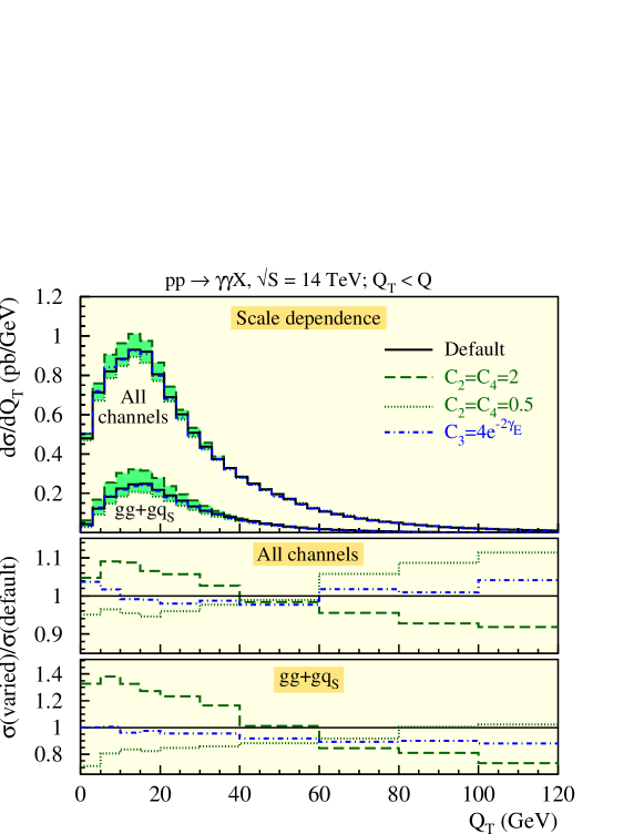
Figure 9: Scale dependence in the $gg+gq_{S}$ and all scattering channels at the LHC for the same scale choices as in Fig. 6.

The scale dependence at the LHC, presented in Fig. 9, is somewhat reduced compared to the Tevatron (cf. Fig. 6). Maximum scale variations of about 40% in the $gg+gq_{S}$ channel are observed at the peak of the $d\sigma/dQ_{T}$ distribution, and they are substantially smaller at large $Q_{T}$. The scale variation in the sum over all channels does not exceed 10% (15%) at small $Q_{T}$ (large $Q_{T}$). Variations in the integrated inclusive rate at $Q>50$ GeV are below 7% (30%) in all channels ($gg+gq_{S}$ channel).

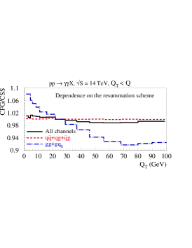
(a)

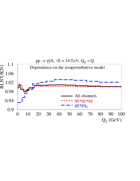
(b)

Figure 10: Same as Fig. 7, at the LHC.

The dependence on the resummation scheme is mild at the LHC (cf. Fig. 10(a)), with the maximal differences between the CSS and CFG schemes below 0.5%, 10%, and 2% in $q\bar{q}+qg$, $gg+gq_{S}$, and all channels. The scheme dependence is again the largest in the $gg+gq_{S}$ channel, where it persists up to the point of switching to the fixed-order cross section at $Q_{T}\approx 120$ GeV. The ratios of the resummed cross sections calculated in the BLNY and KN1 models for nonperturbative contributions in the CSS scheme are shown in Fig. 10(b). The influence of the long-distance (large-$b)$ contributions is suppressed at the high center-of-mass energy of the LHC. Differences between the predictions in the two models do not exceed 2%, 6%, and 2% in the $q\bar{q}+qg,$ $gg+gq_{S},$ and all scattering channels.

The KN1 and BLNY nonperturbative models neglect the possibility of a strong $x$ dependence of the nonperturbative function, which may substantially modify our predictions at the energy of the LHC collider. Analysis of small-$x$ semi-inclusive deep inelastic scattering data Berge et al. (2005) suggests that $x$-dependent nonperturbative corrections of uncertain magnitude may substantially affect the resummed cross sections. Such corrections can be constrained by studying the rapidity and energy dependence of the nonperturbative function at the Tevatron and LHC, for example, from copious production of $Z$ bosons Berge et al. (2005). We conclude that uncertainties due to the choice of the resummation scheme and the nonperturbative model will be small at the LHC, if the resummed nonperturbative function does not vary strongly with $x$.

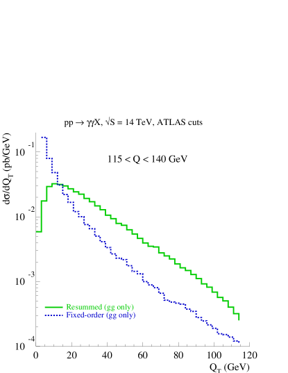
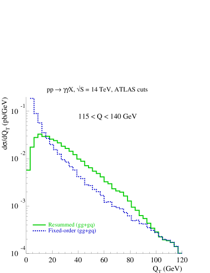
(a)                                                                  (b)

Figure 11: Inclusion of the $qg$ contribution improves the matching of the resummed and NLO perturbative cross sections at large $Q_{T}$, as demonstrated by these plots of the resummed and finite-order NLO cross sections for (a) the $gg$ channel only; (b) the combined $gg+gq_{S}$ channel. The resummed and NLO cross sections are shown by the solid and dashed lines.

IV.3 The role of the $gq_{S}$ contribution

Figures 5-10 show the contributions from the $q\bar{q}+qg$ and $gg+gq_{S}$ channels along with their sum. One may wonder if a further decomposition into $q\bar{q}$ and $qg$ (or $gg$ and $gq_{S}$) contributions could provide additional insights into the relative importance of different scattering processes. We observe in our calculations that the resummed cross sections $W+Y$ and the fixed-order cross sections $P$ in the elementary scattering subchannels ($q\bar{q}$, $qg$,…) may not cross until $Q_{T}$ is significantly larger than $Q$. This result is at variance with our expectation that the fixed-order answer should be adequate when $Q_{T}$ is of order $Q$, where logarithmic effects are small, and the one-scale nature of the dynamics seems apparent.

Consider, for example, the $gg$ and $gg+gq_{S}$ transverse momentum distributions in the mass interval $115<Q<140$ GeV at the LHC shown in Figs. 11(a) and (b). In the $gg$ channel alone (Fig. 11(a)), the $W+Y$ cross section remains above the NLO cross section $P$ until $Q_{T}\sim 140\mbox{ GeV}$. However, after the $gq_{S}$ contribution is included (Fig. 11(b)), $W+Y$ crosses $P$ at $Q_{T}\sim 105\mbox{ GeV}$. Our expectation of the adequacy of the NLO prediction at $Q_{T}\sim Q$ is satisfied in this case, and this conclusion also holds for other intervals of $Q$. At the crossing point, the two cross sections satisfy $W+Y=P,$ i.e., $W=A$; the resummed term is equal to its NLO perturbative expansion, the asymptotic term. Similarly, good matching of the resummed and NLO cross sections in the $q\bar{q}+qg$ channel requires that we include both $q\bar{q}$ and $qg$ contributions.

This feature can be understood by noticing that the flavors of the PDF’s $f_{a/h}(x,\mu)$ mix in the process of PDF evolution. Consequently the perturbative expansion of $W$ in the $gg$ channel contains the full NLO asymptotic piece $A$ in the combined $gg+gq_{S}$ channel, generated from the Sudakov exponential and lowest-order resummed contribution $\propto f_{g/h_{1}}(x_{1},1/b)\,f_{g/h_{2}}(x_{2},1/b)$ evaluated at a scale of order $1/b$. The mismatch between the flavor content in the perturbatively expanded $W$ and $A$ in nominally the same $gg$ subchannel causes the difference $W-A$ to be large and delays the crossing. On the other hand, the flavor content of $W$ and $A$ is the same (up to NNLO) when the $gg$ and $gq_{S}$ contributions are combined, and the matching is improved. The $gq_{S}$ scattering subchannel has been assumed to be small and neglected in past studies, and indeed it contributes about one tenth of the $gg+gq_{S}$ inclusive rate $d\sigma/dQ$. However, we see that the $gq_{S}$ contribution must be included to correctly predict $d\sigma/dQ_{T}$ and to realize matching between the resummed and perturbative contributions at large transverse momenta.

V Summary and Conclusions

In this paper, we address new theoretical issues in $Q_{T}$ resummation at two-loop accuracy that arise in the gluon-gluon subprocess, $gg+gq\rightarrow\gamma\gamma$, one of the important short-distance subprocesses that contribute to the inclusive reactions $p\bar{p}\rightarrow\gamma\gamma X$ at the Fermilab Tevatron and $pp\rightarrow\gamma\gamma X$ at the CERN Large Hadron Collider (LHC).

We evaluate all next-to-leading (NLO) contributions of order ${\mathcal{O}}(\alpha^{2}\alpha_{s}^{3})$ to the $gg+gq\rightarrow\gamma\gamma$ process (Fig. 1(b-e)). A new ingredient in this paper is the inclusion of the $gq\rightarrow\gamma\gamma q$ process, Fig. 1(d), a necessary component of the resummed NLO contribution. We resum to next-to-next-to-leading logarithmic (NNLL) accuracy the large logarithmic terms of the form $\ln(Q_{T}^{2}/Q^{2})$ in the limit when $Q_{T}$ of the $\gamma\gamma$ pair is smaller than its invariant mass $Q$. The perturbative Sudakov functions ${\mathcal{A}}$ and ${\mathcal{B}}$ and the Wilson coefficient functions ${\mathcal{C}}$ in the resummed cross section $W$ are computed to orders $\alpha_{s}^{3},$ $\alpha_{s}^{2}$, and $\alpha_{s}$. The resummed cross sections are computed according to the CSS Collins et al. (1985) and CFG Catani et al. (2001) resummation schemes, with the differences between the two approaches reflecting the size of higher-order corrections. A new nonperturbative function Konychev and Nadolsky (2006), dominated by a process-independent soft correction, is employed to describe the dynamics at large impact parameters.

Subtraction of the singular logarithmic contributions associated with initial-state radiation from the NLO cross section $P$ defines a regular piece $Y$. This regular term is added to the small-$Q_{T}$ resummed cross section $W$ to predict the production rate at small to moderate values of $Q_{T}$. In the $gg$ channel, we also subtract from $P$ a new singular spin-flip contribution that affects azimuthal angle ($\varphi_{*})$ dependence in the Collins-Soper reference frame. For our final prediction, we switch from the resummed cross section $W+Y$ to $P$ at the point where $W+Y$ crosses $P$, approaching $P$ from above, as in Ref. Balazs and Yuan (1997). The location of this point in $Q_{T}$ is of order $Q$ in the $q\bar{q}+qg$ and the $gg+gq$ channels. For such matching to happen, it is essential to combine cross sections in the $q\bar{q}$ and $qg$ ($gg$ and $gq$) channels, as demonstrated in Sec. IV.3.

At the LHC (Tevatron), the $gg+gq$ subprocess contributes 20% (10%) of the total $\gamma\gamma$ production rate (integrated over the full range of the photons’ momenta). The relative contribution of $gg+gq$ scattering may reach 25% for some $Q$ and $Q_{T}$ values. The $gg+gq$ channel provides an interesting opportunity to test CSS resummation at a loop level and may be explored in detail at later stages of the LHC operation. The NNLL/NLO resummed cross section for the $gg+gq_{S}$ channel is used in Ref. Balazs et al. (2007) to predict fully differential distributions of Higgs bosons and QCD background at the LHC in the $\mbox{Higgs}\rightarrow\gamma\gamma$ decay mode.

Appendix A The $gq_{S}\rightarrow\gamma\gamma q_{S}$ amplitude

To obtain the gluon-quark contribution to the $gg+gq_{S}$ scattering channel shown in Fig. 1(d), we derive the helicity-dependent $q\bar{q}\gamma\gamma g\rightarrow 0$ amplitude ${\mathcal{M}}_{5}(q_{1},\bar{q}_{2},\gamma_{3},\gamma_{4},g_{5})$ from the one-loop $q\bar{q}ggg$ amplitude in the color-decomposed representation available in Ref. Bern et al. (1995). The $q\bar{q}\gamma\gamma g$ amplitude is expressed as

$${\mathcal{M}}_{5}(q_{1}^{c_{1}},\bar{q}_{2}^{c_{2}},\gamma_{3},\gamma_{4},g_{5}^{a_{5}})=2g^{3}e^{2}\left(\sum_{i_{l}}e_{i_{l}}^{2}\right)T_{c_{1}c_{2}}^{a_{5}}\sum_{\sigma\in S_{3}^{(345)}}A_{5;1}^{L,[1/2]}(1_{q},2_{\bar{q}};\sigma(3),\sigma(4),\sigma(5))$$ (40)

in terms of the primitive amplitudes $A_{5;1}^{L,[1/2]}(1_{q},2_{\bar{q}};3,4,5)=-A_{5;1}^{f}(1_{q},2_{\bar{q}};3,4,5)-A_{5;1}^{s}(1_{q},2_{\bar{q}};3,4,5)$ for $q\bar{q}ggg\rightarrow 0$ scattering involving a spin-1/2 fermion loop. The amplitude ${\mathcal{M}}_{5}$ is proportional to the sum $\sum_{i_{l}}\left(e^{2}e_{i_{l}}^{2}\right)$ of squared quark charges circulating in the fermion loop, as well as the QCD generator matrix $T_{c_{1}c_{2}}^{a_{5}},$ with $\mbox{{Tr}}(T^{a_{1}}T^{a_{2}})=\delta^{a_{1}a_{2}}$. The color indices $c_{1},\,c_{2},$ and $a_{5}$ belong to the quark 1, antiquark 2, and gluon 5. The primitive amplitudes are summed over all possible permutations $S_{3}^{(345)}$ of the legs 3, 4, and 5.

Equation (40) is derived from Eq. (2.10) of Ref. Bern et al. (1995) after gluons 3 and 4 are replaced with photons, i.e., the QCD generators $T^{a_{3}}$and $T^{a_{4}}$ are replaced by identity matrices, and the overall charge factor is adjusted, $g^{5}\rightarrow 2g^{3}\sum_{i_{l}}(ee_{i_{l}})^{2}.$ It correctly reproduces the small-$Q_{T}$ asymptotic behavior reflected in Eq. (16), which we derive by applying factorization relations in the splitting amplitude formalism discussed in Appendix B. The $q\bar{q}\gamma\gamma g$ amplitude in Eq. (40) disagrees with the one published in Ref. Yasui (2002) which appears to violate factorization relations in the $q\parallel\bar{q}$ limit. A few independent amplitudes $A_{5;1}^{f}(1_{q},2_{\bar{q}};3,4,5)$ and $A_{5;1}^{s}(1_{q},2_{\bar{q}};3,4,5)$ are presented explicitly in Sec. 5 of Ref. Bern et al. (1995), with the remaining amplitudes related by discrete symmetries according to Eq. (5.25) in that publication. Some $q\bar{q}ggg$ amplitudes contain infrared poles, which cancel in the sum over permutations $S_{3}^{(345)}$. We retain only non-vanishing finite parts $F^{x}$ of such divergent amplitudes, i.e., we take $A_{5;1}^{x}=iF^{x}/(16\pi^{2})$ for $x=f$ and $s.$

Appendix B Derivation of the small-$Q_{T}$ asymptotic term for gluon-gluon scattering

In this appendix, we derive the small-$Q_{T}$ asymptotic approximation Eq. (16) for the NLO cross section in $g_{1}g_{2}\rightarrow\gamma_{3}\gamma_{4}$ scattering. We expand the finite-order cross section as a series in the small parameter $Q_{T}^{2}/Q^{2}$. Consider first the leading real-emission contributions, which arise when gluon 5 is radiated off the external gluon leg 1 or 2 as in Fig. 1(b). In the notation introduced in Sec. III, the small-$Q_{T}$ approximation for the real-emission cross section takes the form

$$\left.A(Q,Q_{T},y,\Omega_{*})\right|_{real}=\int_{x_{1}}^{1}d\xi_{1}\int_{x_{2}}^{1}d\xi_{2}f_{g/h_{1}}(\xi_{1},\mu_{F})f_{g/h_{2}}(\xi_{2},\mu_{F})\frac{1}{(2\pi)^{4}}\frac{1}{64\xi_{1}\xi_{2}S}\left|{\mathcal{M}}_{5}\right|^{2}$$ (41)

$$\times \left\{\frac{\delta(\xi_{1}-x_{1})}{\left[1-\widehat{x}_{2}\right]_{+}}+\frac{\delta(\xi_{2}-x_{2})}{\left[1-\widehat{x}_{1}\right]_{+}}-x_{1}x_{2}\delta(\xi_{1}-x_{1})\delta(\xi_{2}-x_{2})\ln\frac{Q_{T}^{2}}{Q^{2}}\right\}.$$

The right-hand side of Eq. (41) includes a product of the gluon parton densities $f_{g/h_{i}}(\xi_{1,2},\mu_{F}),$ squares of parton-scattering amplitudes ${\mathcal{M}}_{5}$, and phase-space factors, integrated over the light-cone momentum fractions $\xi_{1,2}\equiv p_{1,2}^{+}/P_{1,2}^{+}$ of the incoming gluons 1 and 2. The delta-functions constrain integration to phase-space regions where the final-state gluon 5 is collinear to gluon 1 [$p_{5}^{\mu}=(1-\widehat{x}_{1})p_{1}^{\mu}$], collinear to gluon 2 [$p_{5}^{\mu}=(1-\widehat{x}_{2})p_{2}^{\mu}$], or soft [$p_{5}^{\mu}\rightarrow 0$], with $\widehat{x}_{i}\equiv x_{i}/\xi_{i}$ for $i=1,2$.

The $2\rightarrow 3$ helicity amplitude ${\mathcal{M}}_{5}(1,2,3,4,5)$ is analyzed conveniently in an unphysical scattering channel $0\rightarrow g(\bar{p}_{1},\bar{\lambda}_{1})g(\bar{p}_{2},\bar{\lambda}_{2})\gamma(\bar{p}_{3},\bar{\lambda}_{3})\gamma(\bar{p}_{4},\bar{\lambda}_{4})g(\bar{p}_{5},\bar{\lambda}_{5})$. The momenta $\bar{p}_{i}$ and helicities $\bar{\lambda}_{i}$ are related to the physical momenta $p_{i}$ and helicities $\lambda_{i}$ as $\{\bar{p}_{i},\bar{\lambda}_{i}\}$=$\{-p_{i},-\lambda_{i}\}$ for $i=1$ or 2, and $\{\bar{p}_{i},\bar{\lambda}_{i}\}$=$\{p_{i},\lambda_{i}\}$ for $i=$3, 4, or 5. ${\mathcal{M}}_{5}(1,2,3,4,5)$ is a shorthand notation for ${\mathcal{M}}_{5}(\bar{p}_{1},\bar{\lambda}_{1};\bar{p}_{2},\bar{\lambda}_{2};\bar{p}_{3},\bar{\lambda}_{3};\bar{p}_{4},\bar{\lambda}_{4};\bar{p}_{5},\bar{\lambda}_{5}).$

The amplitude ${\mathcal{M}}_{5}(1,2,3,4,5)$ was derived in Refs. Balazs et al. (2000); de Florian and Kunszt (1999) from color-decomposed 5-gluon 1-loop scattering amplitudes Bern et al. (1993). ${\mathcal{M}}_{5}(1,2,3,4,5)$ is built from 1-loop partial amplitudes $A_{5;1}(1,2,3,4,5)$ for the $0\rightarrow gg\gamma\gamma g$ scattering process, identical to the partial amplitudes for $0\rightarrow ggggg$ scattering via a spin-1/2 fermion loop Bern et al. (1993). The squared 5-leg amplitude, averaged over spins, colors, and identical final-state particles, is

$$|{\mathcal{M}}_{5}|^{2} = \sigma_{g}^{(1)}\sum_{\bar{\lambda}_{1},\bar{\lambda}_{2},\bar{\lambda}_{3},\bar{\lambda}_{4},\bar{\lambda}_{5}}\Biggl{|}\,\sum_{\sigma\in{\textrm{COP}}_{3}^{(125)}}A_{5;1}(\sigma_{1},\sigma_{2},\sigma_{3},\sigma_{4},\sigma_{5})\Biggr{|}^{2},$$ (42)

with

$$\sigma_{g}^{(1)}\equiv(4\pi)^{5}\alpha_{s}^{3}\alpha^{2}(\sum_{i}e_{i}^{2})^{2}\frac{N_{c}}{N_{c}^{2}-1}.$$ (43)

The partial amplitudes are summed over all permutations $\sigma$ of the external indices (1,2,3,5) with a fixed cyclic ordering of (1,2,5), i.e., cyclically-ordered (COP) permutations:

$$\sum_{\sigma\in{\textrm{COP}}_{3}^{(125)}}A_{5;1}(\sigma_{1},\sigma_{2},\sigma_{3},\sigma_{4},\sigma_{5})\equiv$$

$$\,\,\,A_{5;1}(1,2,5,3,4)+A_{5;1}(1,2,3,5,4)+A_{5;1}(1,3,2,5,4)+A_{5;1}(3,1,2,5,4)+$$

$$\,\,\,A_{5;1}(5,1,2,3,4)+A_{5;1}(5,1,3,2,4)+A_{5;1}(5,3,1,2,4)+A_{5;1}(3,5,1,2,4)+$$

$$\,\,\,A_{5;1}(2,5,1,3,4)+A_{5;1}(2,5,3,1,4)+A_{5;1}(2,3,5,1,4)+A_{5;1}(3,2,5,1,4).$$ (44)

The collinear and soft behaviors of the amplitude ${\mathcal{M}}_{5}$ can be established by following the approach in Refs. Bern et al. (1993, 1994a, 1994b, 1995, 1998, 1999); Kosower and Uwer (1999), extended recently to the two-loop level Bern et al. (2004); Badger and Glover (2004). When gluon 5 is collinear to gluon 1, the amplitude ${\mathcal{M}}_{5}(1,2,3,4,5)$ is dominated by six partial amplitudes with cyclically adjacent indices 5 and 1, such as $A_{5;1}(5,1,2,3,4)$. Similarly, when gluon 5 is collinear to gluon 2, ${\mathcal{M}}_{5}(1,2,3,4,5)$ is dominated by six partial amplitudes with cyclically adjacent indices 2 and 5. Each leading partial amplitude $A_{5;1}(...,5,1,...)$ factors in the $5\parallel 1$ collinear limit into a 4-leg partial amplitude $A_{4;1}(...,I,...)$ for production of 2, 3, 4, and intermediate gluon $I$, and amplitude $\mbox{Split}_{-\bar{\lambda}_{I}}^{tree}(5,1)$ Parke and Taylor (1986); Mangano and Parke (1988); Berends and Giele (1988); Mangano and Parke (1991) describing tree-level splitting of $I$ into 5 and 1:

$$A_{5;1}(...,5,1,...)\stackrel{{\scriptstyle 5\parallel 1}}{{\longrightarrow}}\sum_{\bar{\lambda}_{I}=\pm 1}\mbox{Split}_{-\bar{\lambda}_{I}}^{tree}(5,1)A_{4;1}(...,I,...)+\mbox{ subleading terms. }$$ (45)

The ellipses in Eq. (45) denote the same permutation of indices 2, 3, and 4 in $A_{5;1}$ and $A_{4;1}$. The amplitudes $\mbox{Split}_{-\bar{\lambda}_{I}}^{tree}(5,1)$ are universal functions of the momenta $\bar{p}_{I},$ $\bar{p}_{1},$ and $\bar{p}_{5}$, which in our case satisfy $\bar{p}_{I}\equiv\bar{p}_{1}+\bar{p}_{5},$ $\bar{p}_{1}=(1-z)\bar{p}_{I},$ and $\bar{p}_{5}=z\bar{p}_{I},$ where $z=1-1/\widehat{x}_{1}.$ The right-hand side of Eq. (45) is summed over the helicities $\bar{\lambda}_{I}$ of $I$. The collinear factorization relation applies to any one-loop $n-$leg primitive amplitude $A_{n}^{loop}(1,...n)$:

$$A_{n}^{loop}(...,a,b,...) \stackrel{{\scriptstyle a\parallel b}}{{\longrightarrow}} \sum_{\bar{\lambda}_{I}}\Biggl{[}\mbox{Split}_{-\bar{\lambda}_{I}}^{tree}(a,b)A_{n-1}^{loop}(...,I,...)+\mbox{Split}_{-\bar{\lambda}_{I}}^{loop}(a,b)A_{n-1}^{tree}(...,I,...)\Biggr{]}.$$ (46)

Equation (46) is evaluated here for $n=5$ external legs, along with the condition that the tree primitive amplitude $A_{4}^{tree}$ vanishes in $0\rightarrow gg\gamma\gamma$ process.

Using Eqs. (42), (44), (45), we derive the approximate form for $|{\mathcal{M}}_{5}|^{2}$ in the $5\parallel 1$ limit:

$$\left|{\mathcal{M}}_{5}(1,2,3,4,5)\right|^{2}\stackrel{{\scriptstyle 5\parallel 1}}{{\longrightarrow}}\sigma_{g}^{(1)}\sum_{\bar{\lambda}_{I},\bar{\lambda}_{I}^{\prime}=\pm 1}{\mathcal{M}}_{4}^{*}(\bar{p}_{I},\bar{\lambda}_{I}^{\prime};2,3,4)T_{\bar{\lambda}_{I}^{\prime},\bar{\lambda}_{I}}(\widehat{x}_{1}){\mathcal{M}}_{4}(\bar{p}_{I},\bar{\lambda}_{I};2,3,4).$$ (47)

Here ${\mathcal{\mathcal{M}}}_{4}(I,2,3,4)\equiv\sum_{\sigma\in S_{3}}A_{4;1}(I,\sigma_{2},\sigma_{3},\sigma_{4})$ is the normalized 4-leg amplitude, obtained by summation of the partial amplitudes $A_{4;1}(I,2,3,4)$ over all possible permutations $S_{3}$ of the legs 2, 3, and 4. The amplitude ${\mathcal{M}}_{4}$ and complex-conjugate amplitude ${\mathcal{M}}_{4}^{*}$ are evaluated for independent helicities $\bar{\lambda}_{I}$ and $\bar{\lambda}_{I}^{\prime}$ of $I$. $T_{\bar{\lambda}_{I}^{\prime},\bar{\lambda}_{I}}(\widehat{x}_{1})$ absorbs contributions from the splitting amplitudes:

$$T_{\bar{\lambda}_{I},\bar{\lambda}_{I}^{\prime}}(\widehat{x}_{1}) \equiv \sum_{\bar{\lambda}_{1},\bar{\lambda}_{5}=\pm 1}\left[\mbox{Split}_{-\bar{\lambda}_{I}}^{tree}(\frac{1}{\widehat{x}_{1}};1,5)\right]^{*}\mbox{Split}_{-\bar{\lambda_{I}}^{\prime}}^{tree}(\frac{1}{\widehat{x}_{1}};1,5).$$ (48)

In a basis with $\bar{\lambda}=+1$ and $\bar{\lambda}=-1$, $T_{\bar{\lambda}_{I}^{\prime},\bar{\lambda}_{I}}(x)$ is a matrix of the form

$$T_{\bar{\lambda}_{I},\bar{\lambda}_{I}^{\prime}}(x) = \frac{2C_{A}}{2xp_{1}\cdot p_{5}}\left(\begin{array}[]{cc}\frac{x}{1-x}+\frac{1-x}{x}+x(1-x)&-\frac{1-x}{x}\frac{[51]}{\langle 51\rangle}\\ -\frac{1-x}{x}\frac{\langle 51\rangle}{[51]}&\frac{x}{1-x}+\frac{1-x}{x}+x(1-x)\end{array}\right).$$ (51)

The diagonal entries of $T_{\bar{\lambda}_{I},\bar{\lambda}_{I}^{\prime}}(\widehat{x}_{1})$ give rise to terms proportional to the unpolarized splitting function $P_{g/g}(\widehat{x}_{1})$ in the asymptotic cross section, with

$$P_{g/g}(\widehat{x}_{1})=2C_{A}\left[\frac{\widehat{x}_{1}}{\left(1-\widehat{x}_{1}\right)_{+}}+\frac{1-\widehat{x}_{1}}{\widehat{x}_{1}}+\widehat{x}_{1}(1-\widehat{x}_{1})\right]+\frac{11N_{c}-2N_{f}}{6}\delta(1-\widehat{x}_{1}),$$ (52)

where $N_{f}$ is the number of active quark flavors. The off-diagonal entries give rise to terms proportional to the spin-flip splitting function

$$P_{g/g}^{\prime}(\widehat{x}_{1})=2C_{A}(1-\widehat{x}_{1})/\widehat{x}_{1},$$ (53)

multiplied by the ratio of spinor products $\langle 51\rangle\equiv\langle 5+|1-\rangle$ and $[51]\equiv\langle 5-|1+\rangle$. In a general reference frame, $\langle 51\rangle/[51]$ is a complex phase depending on the azimuthal separation $\varphi_{1}-\varphi_{5}$ between the gluons 1 and 5. In the Collins-Soper frame, this phase reduces to $\langle 51\rangle/[51]=-1$.

Next, we employ explicit expressions for ${\mathcal{M}}_{4}(I,2,3,4)$ from Ref. Bern et al. (2001), given by products ${\mathcal{M}}_{4}(I,2,3,4)=S_{\bar{\lambda}_{I}\bar{\lambda}_{2}\bar{\lambda}_{3}\bar{\lambda}_{4}}M_{\bar{\lambda}_{I}\bar{\lambda}_{2}\bar{\lambda}_{3}\bar{\lambda}_{4}}^{(1)}$ of reduced matrix elements $M_{\bar{\lambda}_{I}\bar{\lambda}_{2}\bar{\lambda}_{3}\bar{\lambda}_{4}}^{(1)}$ and phase factors $S_{\bar{\lambda}_{I}\bar{\lambda}_{2}\bar{\lambda}_{3}\bar{\lambda}_{4}}$. With these expressions inserted, Eq. (47) becomes in the Collins-Soper frame

$$|{\mathcal{M}}_{5}(1,2,3,4,5)|^{2}\stackrel{{\scriptstyle 5\parallel 1}}{{\longrightarrow}}\frac{\sigma_{g}^{(1)}}{2\widehat{x}_{1}p_{1}\cdot p_{5}}\Biggl{\{}P_{g/g}(\widehat{x}_{1})L_{g}(\theta_{*})+P_{g/g}^{\prime}(\widehat{x}_{1})\,L_{g}^{\prime}(\theta_{*})\,\cos 2\varphi_{*}\Biggr{\}},$$ (54)

where

$$L_{g}(\theta_{*})=\sum_{\bar{\lambda}_{1},\bar{\lambda}_{2},\bar{\lambda}_{3},\bar{\lambda}_{4}}\left|M_{\bar{\lambda}_{I}\bar{\lambda}_{2}\bar{\lambda}_{3}\bar{\lambda}_{4}}^{(1)}\right|^{2},$$ (55)

and

$$L_{g}^{\prime}(\theta_{*})=-4\mbox{{Re}}\left\{M_{1,1,-1,-1}^{(1)}+M_{1,-1,1,-1}^{(1)}+M_{-1,1,1,-1}^{(1)}+1\right\}.$$ (56)

In the $5\parallel 2$ collinear limit $\left|{\mathcal{M}}_{5}\right|^{2}$ is

$$|{\mathcal{M}}_{5}(1,2,3,4,5)|^{2}\stackrel{{\scriptstyle 5\parallel 2}}{{\longrightarrow}}\frac{\sigma_{g}^{(1)}}{2\widehat{x}_{2}p_{2}\cdot p_{5}}\Biggl{\{}P_{g/g}(\widehat{x}_{2})\,L_{g}(\theta_{*})+P_{g/g}^{\prime}(\widehat{x}_{2})\,L_{g}^{\prime}(\theta_{*})\,\cos 2\varphi_{*}\Biggr{\}}.$$ (57)

In the soft limit $p_{5}^{\mu}\rightarrow 0$, $\left|{\mathcal{M}}_{5}\right|^{2}$ factors as

$$\left|{\mathcal{M}}_{5}(1,2,3,4,5)\right|^{2}\rightarrow\frac{1}{Q_{T}^{2}}2C_{A}\frac{\alpha_{s}}{\pi}\left|{\mathcal{M}}_{4}(1,2,3,4)\right|^{2}+\mbox{subleading terms.}$$ (58)

Inserting collinear and soft approximations (54), (57), and (58) in Eq. (41) and making some simplifications, we derive the asymptotic expression for real-emission contributions,

$$\left.\frac{d\sigma_{gg}}{dQ^{2}dy\,dQ_{T}^{2}d\Omega_{*}}\right|_{real}\rightarrow\frac{\sigma_{g}^{(0)}}{S}\frac{1}{2\pi Q_{T}^{2}}\frac{\alpha_{s}}{\pi}$$ (59)

$$\times \Biggl{\{}L_{g}(\theta_{*})\biggl{(}f_{g/h_{1}}(x_{1},\mu_{F})f_{g/h_{2}}(x_{2},\mu_{F})\left({\mathcal{A}}_{g}^{(1,c)}\ln\frac{Q^{2}}{Q_{T}^{2}}+{\mathcal{{\mathcal{B}}}}_{g}^{(1,c)}\right)$$

$$+ \left[P_{g/g}\otimes f_{g/h_{1}}\right](x_{1},\mu_{F})\,f_{g/h_{2}}(x_{2},\mu_{F})+f_{g/h_{1}}(x_{1},\mu_{F})\left[P_{g/g}\otimes f_{g/h_{2}}\right](x_{2},\mu_{F})\biggr{)}$$

$$+ \cos 2\varphi_{*}L_{g}^{\prime}(\theta_{*})\biggl{(}\left[P_{g/g}^{\prime}\otimes f_{g/h_{1}}\right](x_{1},\mu_{F})\,f_{g/h_{2}}(x_{2},\mu_{F})$$

$$+ f_{g/h_{1}}(x_{1},\mu_{F})\left[P_{g/g}^{\prime}\otimes f_{g/h_{2}}\right](x_{2},\mu_{F})\biggr{)}\Biggr{\}}.$$

Once we add the two-loop 4-leg virtual corrections [Fig. 1(e)], the soft singularities in the real-emission cross section residing at $Q_{T}=0$ are canceled Bern et al. (2002); Nadolsky and Schmidt (2003). The final small-$Q_{T}$ expression coincides with Eq. (16).

References

- Collins et al. (1985) J. C. Collins, D. E. Soper, and G. Sterman, Nucl. Phys. B250, 199 (1985).
- ATLAS Collaboration (1999) ATLAS Collaboration, ATLAS detector and physics performance. Technical design report. Vol. 2 (1999), CERN-LHCC-99-15.
- CMS Collaboration (2006) CMS Collaboration, CMS physics. Technical design report. Vol. 2 (2006), CERN-LHCC 2006-021.
- Abdullin et al. (2005) S. Abdullin et al., Eur. Phys. J. C39S2, 41 (2005).
- Balazs et al. (2006) C. Balazs, E. L. Berger, P. Nadolsky, and C. P. Yuan, Phys. Lett. B637, 235 (2006).
- Balazs et al. (2007) C. Balazs, E. L. Berger, P. M. Nadolsky, and C. P. Yuan (2007), eprint arXiv:0704.0001 [hep-ph].
- Balazs et al. (1998) C. Balazs, E. L. Berger, S. Mrenna, and C.-P. Yuan, Phys. Rev. D57, 6934 (1998).
- Bern et al. (1995) Z. Bern, L. J. Dixon, and D. A. Kosower, Nucl. Phys. B437, 259 (1995).
- Bern et al. (1993) Z. Bern, L. J. Dixon, and D. A. Kosower, Phys. Rev. Lett. 70, 2677 (1993).
- Bern et al. (1994a) Z. Bern, G. Chalmers, L. J. Dixon, and D. A. Kosower, Phys. Rev. Lett. 72, 2134 (1994a).
- Bern et al. (1994b) Z. Bern, L. J. Dixon, D. C. Dunbar, and D. A. Kosower, Nucl. Phys. B425, 217 (1994b).
- Bern et al. (1998) Z. Bern, V. Del Duca, and C. R. Schmidt, Phys. Lett. B445, 168 (1998).
- Bern et al. (1999) Z. Bern, V. Del Duca, W. B. Kilgore, and C. R. Schmidt, Phys. Rev. D60, 116001 (1999).
- Kosower and Uwer (1999) D. A. Kosower and P. Uwer, Nucl. Phys. B563, 477 (1999).
- Collins and Soper (1977) J. C. Collins and D. E. Soper, Phys. Rev. D16, 2219 (1977).
- Aurenche et al. (1985) P. Aurenche, A. Douiri, R. Baier, M. Fontannaz, and D. Schiff, Z. Phys. C29, 459 (1985).
- Bailey et al. (1992) B. Bailey, J. F. Owens, and J. Ohnemus, Phys. Rev. D46, 2018 (1992).
- Binoth et al. (2000) T. Binoth, J. P. Guillet, E. Pilon, and M. Werlen, Eur. Phys. J. C16, 311 (2000).
- Berger et al. (1984) E. L. Berger, E. Braaten, and R. D. Field, Nucl. Phys. B239, 52 (1984).
- Balazs et al. (2000) C. Balazs, P. Nadolsky, C. Schmidt, and C.-P. Yuan, Phys. Lett. B489, 157 (2000).
- de Florian and Kunszt (1999) D. de Florian and Z. Kunszt, Phys. Lett. B460, 184 (1999).
- Bern et al. (2001) Z. Bern, A. De Freitas, and L. J. Dixon, JHEP 09, 037 (2001).
- Bern et al. (2002) Z. Bern, L. J. Dixon, and C. Schmidt, Phys. Rev. D66, 074018 (2002).
- Yasui (2002) Y. Yasui, Phys. Rev. D66, 094012 (2002).
- Catani and Seymour (1997) S. Catani and M. H. Seymour, Nucl. Phys. B485, 291 (1997).
- Collins and Soper (1981) J. C. Collins and D. E. Soper, Nucl. Phys. B193, 381 (1981).
- Collins and Soper (1982a) J. C. Collins and D. E. Soper, Nucl. Phys. B197, 446 (1982a).
- Ralston and Soper (1979) J. P. Ralston and D. E. Soper, Nucl. Phys. B152, 109 (1979).
- Soper (1977) D. E. Soper, Phys. Rev. D15, 1141 (1977).
- Soper (1979) D. E. Soper, Phys. Rev. Lett. 43, 1847 (1979).
- Ali and Hoodbhoy (1993) R. Ali and P. Hoodbhoy, Z. Phys. C57, 325 (1993).
- Bashinsky and Jaffe (1998) S. V. Bashinsky and R. L. Jaffe, Nucl. Phys. B536, 303 (1998).
- Collins and Soper (1982b) J. C. Collins and D. E. Soper, Nucl. Phys. B194, 445 (1982b).
- Mulders and Rodrigues (2001) P. J. Mulders and J. Rodrigues, Phys. Rev. D63, 094021 (2001), and references therein.
- Dokshitzer (1977) Y. L. Dokshitzer, Sov. Phys. JETP 46, 641 (1977).
- Gribov and Lipatov (1972a) V. N. Gribov and L. N. Lipatov, Sov. J. Nucl. Phys. 15, 438 (1972a).
- Gribov and Lipatov (1972b) V. N. Gribov and L. N. Lipatov, Sov. J. Nucl. Phys. 15, 675 (1972b).
- Altarelli and Parisi (1977) G. Altarelli and G. Parisi, Nucl. Phys. B126, 298 (1977).
- Tangerman and Mulders (1995) R. D. Tangerman and P. J. Mulders, Phys. Rev. D51, 3357 (1995), and references therein.
- Henneman et al. (2002) A. A. Henneman, D. Boer, and P. J. Mulders, Nucl. Phys. B620, 331 (2002).
- Boer (2001) D. Boer, Nucl. Phys. B603, 195 (2001).
- Idilbi et al. (2004) A. Idilbi, X. Ji, J.-P. Ma, and F. Yuan, Phys. Rev. D70, 074021 (2004).
- Nadolsky and Schmidt (2003) P. M. Nadolsky and C. R. Schmidt, Phys. Lett. B558, 63 (2003).
- Yuan (1992) C.-P. Yuan, Phys. Lett. B283, 395 (1992).
- Vogt et al. (2004) A. Vogt, S. Moch, and J. A. M. Vermaseren, Nucl. Phys. B691, 129 (2004).
- Balazs and Yuan (1997) C. Balazs and C.-P. Yuan, Phys. Rev. D56, 5558 (1997).
- Catani et al. (2001) S. Catani, D. de Florian, and M. Grazzini, Nucl. Phys. B596, 299 (2001).
- Berger and Qiu (2003) E. L. Berger and J. Qiu, Phys. Rev. D67, 034026 (2003).
- Konychev and Nadolsky (2006) A. V. Konychev and P. M. Nadolsky, Phys. Lett. B633, 710 (2006).
- Landry et al. (2003) F. Landry, R. Brock, P. M. Nadolsky, and C.-P. Yuan, Phys. Rev. D67, 073016 (2003).
- Ladinsky and Yuan (1994) G. A. Ladinsky and C.-P. Yuan, Phys. Rev. D50, 4239 (1994).
- Balazs (1999) C. Balazs (1999), eprint hep-ph/9906422.
- Acosta et al. (2005) D. Acosta et al. (CDF Collaboration), Phys. Rev. Lett. 95, 022003 (2005).
- Harlander and Kilgore (2002) R. V. Harlander and W. B. Kilgore, Phys. Rev. Lett. 88, 201801 (2002).
- Anastasiou et al. (2004) C. Anastasiou, K. Melnikov, and F. Petriello, Phys. Rev. Lett. 93, 262002 (2004).
- Anastasiou et al. (2005) C. Anastasiou, K. Melnikov, and F. Petriello, Nucl. Phys. B724, 197 (2005).
- Berge et al. (2005) S. Berge, P. Nadolsky, F. Olness, and C.-P. Yuan, Phys. Rev. D72, 033015 (2005).
- Binosi and Theussl (2004) D. Binosi and L. Theussl, Comput. Phys. Commun. 161, 76 (2004).
- Bern et al. (2004) Z. Bern, L. J. Dixon, and D. A. Kosower, JHEP 08, 012 (2004).
- Badger and Glover (2004) S. D. Badger and E. W. N. Glover, JHEP 07, 040 (2004).
- Parke and Taylor (1986) S. J. Parke and T. R. Taylor, Phys. Rev. Lett. 56, 2459 (1986).
- Mangano and Parke (1988) M. L. Mangano and S. J. Parke, Nucl. Phys. B299, 673 (1988).
- Berends and Giele (1988) F. A. Berends and W. T. Giele, Nucl. Phys. B306, 759 (1988).
- Mangano and Parke (1991) M. L. Mangano and S. J. Parke, Phys. Rept. 200, 301 (1991).
- (65) L. Dixon, private communication.
- de Florian and Grazzini (2000) D. de Florian and M. Grazzini, Phys. Rev. Lett. 85, 4678 (2000).
- Moch et al. (2004) S. Moch, J. A. M. Vermaseren, and A. Vogt, Nucl. Phys. B688, 101 (2004).