We investigate the little hierarchy between $Z$ boson mass and the SUSY breaking scale in the context of landscape of electroweak symmetry breaking vacua. We consider the radiative symmetry breaking and found that the scale where the electroweak symmetry breaking conditions are satisfied and the average stop mass scale is preferred to be very close to each other in spite of the fact that their origins depend on different parameters of the model. If the electroweak symmetry breaking scale is fixed at about 1 TeV by the supersymmetry model parameters then the little hierarchy seems to be preferred among the electroweak symmetry breaking vacua. We characterize the little hierarchy by a probability function and the mSUGRA model is used as an example to show the 90% and 95% probability contours in the experimentally allowed region. We also investigate the size of the Higgsino mass $\mu$ by considering the distribution of electroweak symmetry breaking scale.

1 Introduction

One of the key motivations for supersymmetric (SUSY) extension of the Standard Model (SM) is the stabilization of the large hierarchy between the Planck scale and the weak scale. Although the SM particle spectrum gets doubled in the SUSY extension, these new particles around the weak scale add an additional attraction for SUSY theories by unifying gauge couplings at the grand unified scale [1]. However, the new particles are not yet to be seen. Neither the LEP nor the Tevatron is successful so far in their attempts to discover these particles, and the search attempts have already exceeded the $Z$ boson mass scale. The SUSY extension which is invoked to explain the electroweak scale seems to require most of the superpartners above the electroweak scale. In the SUSY breaking models mediated by minimal supergravity (mSUGRA) [2, 3], where the squarks and sleptons masses are unified at the GUT scale, the average stop mass scale is about 1 TeV or above. Question now arises regarding the justification of the heavy superpartner masses. Can this little hierarchy between the $Z$ boson mass and the superpartner masses be rationalized in these models?

We need to understand first the relation between the SUSY breaking masses and the $Z$ boson mass. The electroweak symmetry breaking relates the SUSY breaking mass scale to the $Z$ boson mass, $M_{Z}$. At the tree level, the minimization of the Higgs potential gives rise to $M_{Z}^{2}/2\simeq-m_{H_{u}}^{2}-\mu^{2}$ in the large $\tan\beta$ limit, where $m_{H_{u}}$ is the SUSY breaking mass for up-type Higgs boson, and $\mu$ is the Higgsino mass which is the coefficient of the bilinear term in the superpotential. Since $|m_{H_{u}}|$ is of the order of the stop mass scale, the natural expectation is that $M_{Z}$ is as large as stop mass, unless there is a cancellation. One can quantify the amount of cancellation by a sensitivity function and finds that smaller $\mu$ (and therefore small $|m_{H_{u}}|$) is needed [4]. One can then conclude that the hierarchy between the SUSY breaking mass scale and $Z$ boson mass is not preferred unless $\mu^{2}$ and $m_{H_{u}}^{2}$ are related in a given SUSY breaking model. This is called naturalness of the electroweak symmetry breaking.

In order to determine the possible location of the SUSY breaking mass scale, we need to go back to the origin of the SUSY models. The SUSY models are expected to arise from well motivated string theory. String theory has many vacua and one expects to have wide range of possibilities of the SUSY model parameters in these vacua [5]. The SUSY parameters can be the vacuum expectation values (VEVs) of the moduli fields. Many of these vacua can give rise to the SUSY extension of the SM where the electroweak symmetry is broken. One can then ask about the distribution of the model parameters in these vacua once the requirement is made that the electroweak symmetry has to be broken. Can one understand the hierarchy between the SUSY breaking mass scale and the $Z$ boson mass from the distribution of the model parameters? One can also ask whether the same conclusion as naturalness holds if a distribution function of the $|M_{Z}/m_{H_{u}}|$ hierarchy is considered. The distribution functions are needed more than the sensitivity function in the context of statistics of vacua.

So far we did not include the features of radiative symmetry breaking [6] in our discussion. Since the theory is not finite, one needs to care about large log correction in the symmetry breaking conditions. The SUSY breaking mass squared, $m_{H_{u}}^{2}$, is driven to be negative at low energy by the renormalization group flow and that leads us to satisfy the electroweak symmetry breaking condition. The radiative symmetry breaking connects the stop mass scale to the $Z$ boson mass in the following way. The symmetry breaking condition (i.e., $-m_{H_{u}}^{2}-\mu^{2}>0$) is satisfied at a scale $Q_{0}$. The tree-level $Z$ boson mass, $M_{Z}^{2}(Q)\simeq-2(m_{H_{u}}^{2}+\mu^{2})(Q)$, depends on the renormalization scale, $Q$. The proper $Z$ boson mass is given approximately at the averaged stop mass scale $Q_{\tilde{t}}$ where the correction from 1-loop Higgs potential is negligible. Those two scales, $Q_{0}$ and $Q_{\tilde{t}}$, are unrelated in general, and the electroweak symmetry is broken when $Q_{0}>Q_{\tilde{t}}$. Now expanding the tree-level $Z$ boson mass, $M_{Z}(Q)$, around the scale $Q_{0}$, one gets $M_{Z}^{2}\propto\ln(Q_{0}/Q_{\tilde{t}})$. Consequently, the scales $Q_{0}$ and $Q_{\tilde{t}}$ need to be close by when the average stop mass is about 1 TeV. So instead of looking for a reason to explain the smallness of $|M_{Z}/m_{H_{u}}|$, we need to understand the proximity of the scales $Q_{0}$ and $Q_{\tilde{t}}$. We therefore direct our investigation to the distribution of the scales $Q_{0}$ and $Q_{\tilde{t}}$ in the context of the statistics of vacua.

We consider the distribution of the hierarchy between $M_{Z}$ and $Q_{\tilde{t}}$, and determine the distribution function assuming that the any SUSY breaking vacuum is equally probable. We determine whether the proximity of $Q_{0}$ and $Q_{\tilde{t}}$ is natural in a large number of vacua. If this closeness is enough probable in the landscape of the electroweak symmetry breaking vacua, the hierarchy between the SUSY breaking scale and $M_{Z}$ can easily be rationalized when $Q_{0}$ is at TeV scale due to a model parameter. It is also interesting to determine the sensitivity function of the $Q_{0}/Q_{\tilde{t}}$ hierarchy and compare it with the distribution function. We also determine the probability of a given hierarchy between the $Q_{\tilde{t}}$ and $M_{Z}$ in mSUGRA model and show 90% and 95% probability contour in the experimentally allowed parameter space. The average of the $\ln(Q_{0}/Q_{\tilde{t}})$ is considered in a recent reference [7] in the context of multiple vacua and it was shown that the $Q_{0}$ should be close to $Q_{\tilde{t}}$ scale. We propose to use the probability function to describe the amount of little hierarchy in this paper.

It is not only interesting to investigate the distribution of $Q_{\tilde{t}}$ to understand the little hierarchy, but also important to investigate the size of other parameters, especially the size of $\mu$, which is claimed to be small for naturalness. To investigate the size of $\mu$, there is another important scale $Q_{H}$ in addition to the scales $Q_{0}$ and $Q_{\tilde{t}}$. The $Q_{H}$ is the scale where $m_{H_{u}}^{2}$ becomes negative. By definition, $Q_{\tilde{t}}<Q_{0}<Q_{H}$ for the electroweak symmetry breaking vacua. The hierarchy between $Q_{0}$ and $Q_{H}$ determines the preferred size of $\mu$ and therefore the size of $\mu$ can be understood for the distribution of $Q_{0}/Q_{H}$. To obtain “natural vacua” (or small $\mu$), all three scales need to be close by. It is also interesting to inquire about whether there are lots of natural vacua among the landscape of electroweak breaking vacua varying the model parameters.

The paper is organized as follows. In section 2, we address the little hierarchy problem. In section 3, we discuss the conditions of the electroweak symmetry breaking and determine the sensitivity function of little hierarchy. In section 4, we describe the little hierarchy problem in the landscape of electroweak vacua and determine the probability function of little hierarchy. We also determine the 90% and 95% probability contours in the mSUGRA model including the experimental constraints. In section 5, we discuss the landscapes of different scale associated with the electroweak symmetry breaking vacua and study the possible size of $\mu$, and section 6 contains our conclusion.

2 Little Hierarchy Problem

The little hierarchy problem is often described by using a sensitivity function [4]. One can quantify the fine-tuning in the minimization condition of Higgs potential by the sensitivity function and concludes that small Higgsino mass $\mu$ is needed for natural electroweak symmetry breaking. However, distribution functions are more appropriate rather than the sensitivity function in the context of statistics of vacua. In this section, we discuss the distribution function of the hierarchy for the tree-level condition to see whether the same conclusion also holds.

The tree-level Higgs potential is given as

$$V=m_{1}^{2}|H_{d}|^{2}+m_{2}^{2}|H_{u}|^{2}+(m_{3}^{2}H_{d}\cdot H_{u}+h.c.)+\frac{g_{2}^{2}+g^{\prime 2}}{8}(|H_{d}|^{2}-|H_{u}|^{2})^{2}+\frac{g_{2}^{2}}{2}(H_{u}^{\dagger}H_{d})(H_{d}^{\dagger}H_{u})\,.$$ (1)

The quartic term is obtained by $D$-term and thus the coupling is related to the gauge couplings. The quadratic terms are given by SUSY breaking Higgs masses, $m_{H_{d}}^{2}$ and $m_{H_{u}}^{2}$, Higgsino mass $\mu$ and SUSY breaking bilinear Higgs mass $B\mu$ : $m_{1}^{2}=m_{H_{d}}^{2}+\mu^{2}$, $m_{2}^{2}=m_{H_{u}}^{2}+\mu^{2}$ and $m_{3}^{2}=B\mu$.

Minimizing the Higgs potential by Higgs VEVs ($v_{d}=\langle H_{d}^{0}\rangle$, $v_{u}=\langle H_{u}^{0}\rangle$), we obtain

$$\frac{M_{Z}^{2}}{2}=\frac{m^{2}_{1}-m^{2}_{2}\tan^{2}\beta}{\tan^{2}\beta-1}\,,\qquad\sin 2\beta=\frac{2|m_{3}^{2}|}{m^{2}_{1}+m^{2}_{2}}\,,$$ (2)

where $\tan\beta=v_{u}/v_{d}$. The conditions of electroweak symmetry breaking at tree-level are

$$m_{1}^{2}\,m_{2}^{2}<(m_{3}^{2})^{2}\,,$$ (3)

$$m_{1}^{2}+m_{2}^{2}>2|m_{3}^{2}|\,,$$ (4)

which corresponds to the conditions $M_{Z}^{2}>0$ and $\sin 2\beta<1$ in Eq.(2). The second condition is obtained by the stabilization of the Higgs potential along the flat direction, $|v_{u}|=|v_{d}|$. The $Z$ boson mass can be expressed as

$$\frac{M_{Z}^{2}}{2}=-\mu^{2}+\frac{m^{2}_{H_{d}}-m^{2}_{H_{u}}\tan^{2}\beta}{\tan^{2}\beta-1}\simeq-\mu^{2}-m_{H_{u}}^{2}\,.$$ (5)

In the radiative electroweak symmetry breaking scenario [6], the condition Eq.(3) is satisfied at the weak scale by renormalization group equation (RGE). The SUSY breaking scalar mass squared for up-type Higgs, $m^{2}_{H_{u}}$, is driven to a negative value by large top Yukawa coupling. Naively, $-m_{H_{u}}^{2}$ is of the same order as the stop and gluino masses at weak scale (especially, when the SUSY breaking scalar masses are assumed to be universal), and consequently, the $Z$ boson mass is of the same order as the SUSY particles. The colored particles are expected to be heavier than sleptons, wino and bino due to the RGE effects using naive boundary conditions at the Planck or the GUT scale. In other word, the uncolored SUSY particles should have been observed in LEP2 experiment. Non-observation of the uncolored superparticles leads stop and gluino masses to be much heavier than the $Z$ boson mass (especially when the gaugino masses are unified at the GUT scale). Moreover, the lightest Higgs mass bound ($m_{h}>114.4$ GeV) pushes up the stop mass or the trilinear scalar coupling for stop $A_{t}$.

Surely, there is a freedom of cancellation in Eq.(5), and there is no problem with the electroweak symmetry breaking even if SUSY particles are much heavier than the mass of the $Z$ boson. However, the cancellation seems unnatural as can be seen in the following discussion.

The sensitivity function to measure the fine-tuning is defined as [4]

$$\Delta[f(x)]\equiv\left|\frac{\partial\ln f}{\partial\ln x}\right|^{-1}.$$ (6)

When $\Delta[f(x)]$ is small, the function $f$ is sensitive to $x$ and the degree of fine-tuning is large. The sensitivity for the $Z$ boson mass is calculated from Eq.(5) as $\Delta[M_{Z}(\mu)]=M_{Z}^{2}/(2\mu^{2})$. The $\mu$ parameter needs to be small to generate less sensitivity. This is the usual naturalness statement. When

$$M_{H}^{2}\equiv(m_{H_{d}}^{2}-m_{H_{u}}^{2}\tan^{2}\beta)/(\tan^{2}\beta-1)$$ (7)

is much larger than the $Z$ boson mass, the fine-tuning is severe. For example, when $M_{H}=500$ GeV, the sensitivity $\Delta[M_{Z}(\mu)]$ is about 2%.

In order to describe the SUSY parameters in terms of the statistics of vacua, in this paper, we suggest that the distribution function and the probability function are more appropriate rather than the sensitivity function.

Let us calculate the distribution function of the $M_{Z}$-$M_{H}$ hierarchy ($r_{H}\equiv M_{Z}/M_{H}$). Assume that any Higgsino mass $\mu$ is equally probable ($D[\mu]={\rm const}$). Then one obtains the distribution function of $r_{H}$ as

$$D[r_{H}]=\frac{r_{H}}{2\sqrt{1-\frac{r_{H}^{2}}{2}}}\,,$$ (8)

by using the relation $dP=D[r_{H}]dr_{H}=D[\mu]d\mu$. The distribution function is normalized to make $\displaystyle\int_{0}^{\sqrt{2}}D[r_{H}]dr_{H}=1$. Since the distribution function looks different by measure, we should use the probability function by integrating the distribution function to avoid a bias for the choice of measure. The probability for $r_{H}>r_{0}$ is given as

$$P[r_{H}>r_{0}]=\int_{r_{H}}^{\sqrt{2}}D[r_{H}]dr_{H}=\sqrt{1-\frac{r_{0}^{2}}{2}}.$$ (9)

So, the probability for $M_{H}<2M_{Z}$ is calculated to be 93%. The probability for $M_{H}>200$ GeV (500 GeV) is only about 5% (1%).

Since the $\mu$ parameter is complex in general, the proper distribution function of $\mu$ may be $D[|\mu|^{2}]={\rm const}$ (or $D[\mu]\propto\mu$) if any complex value is equally probable. In this case, the distribution function is $D[r_{H}]=r_{H}$ and the probability function is $P[r_{H}<r_{0}]=r_{0}^{2}/2$. The probability function can be written as $M_{Z}^{2}/(2M_{H}^{2})$ which naively corresponds to $\Delta[M_{Z}(\mu)]$. The probability for fine-tuning is relaxed than before: The probability for $M_{H}>200$ GeV (500 GeV) is about 10% (2%). We note that the complex $\mu$ does not mean CP violation directly since the phase of $\mu$ can be rotated out by the field redefinition of Higgs fields when $B$ parameter is real.

More generically, the probability function is

$$P[r_{H}<r_{0}]=1-\left(1-\frac{r_{0}^{2}}{2}\right)^{\frac{m}{2}},$$ (10)

when $D[\mu^{m}]={\rm const}$, and the probability can be written approximately $m{M_{Z}^{2}}/(4{M_{H}}^{2})$ in the fine-tune region, which naively corresponds to the sensitivity function of $\Delta[M_{Z}(\mu^{m/2})]$. Therefore, naturalness statement holds and the little hierarchy is not rationalized even if we use the probability function when $\mu$ is distributed.

There are mainly two directions to solve the little hierarchy problem. In one direction one needs to select a suitable mass spectrum of SUSY particles at low energy. For example, if squark, sleptons and wino are naturally heavier than the SUSY breaking Higgs mass $M_{H}$ in a SUSY model, the LEP2 experiments do not conflict with the fine-tuning. In this case, a favorable SUSY breaking scenario will be chosen such as mirage mediation model [8, 9].

The other direction is to reconsider the distribution of $\mu$ parameter and to see what is a suitable parameter to distribute in order to discuss the fine-tuning in electroweak symmetry breaking. In this paper, we investigate this direction.

3 Conditions of Radiative Electroweak Symmetry Breaking

In the previous section, we only study tree-level conditions, Eq.(2), which do not include the conditions that the symmetry breaking is radiatively induced. Let us describe the conditions of the radiative electroweak symmetry breaking.

As we discussed, it seems that the fine-tuning is needed in Eq.(5) and the fine-tuning has less probability. At what scale do we need the fine-tuning? Since the mass parameters are running, we have to fix the scale where we need fine-tuning. The minimization conditions, Eq.(2), are given in the tree level for a given scale $Q$. There exists a 1-loop corrected potential [10],

$$\Delta V^{\rm 1-loop}=\frac{1}{64\pi^{2}}\sum_{J}(-1)^{2J}(2J+1)m_{J}^{4}\left(\ln\frac{m_{J}^{2}}{Q^{2}}-\frac{3}{2}\right)\,,$$ (11)

where $J$ is a spin of the matter. Since $m_{J}$ depends on the Higgs VEVs, we need to include the derivatives of 1-loop potential in minimization of the Higgs potential. We can use a scheme that the scale $Q$ is chosen to make the derivatives of 1-loop potential $\partial\Delta V/\partial v_{u,d}$ to be small [11]. One can find that the scale is a geometrical average of the stop mass, $Q_{\tilde{t}}\equiv(m_{\tilde{t}_{1}}m_{\tilde{t}_{2}})^{1/2}$. As a result, the tree-level relations Eq.(2) are approximately satisfied at the scale $Q_{\tilde{t}}$, and the electroweak symmetry breaking conditions Eqs.(3,4) need to be satisfied at $Q_{\tilde{t}}$. Defining the scale where the electroweak symmetry is broken (Eq.(3) is satisfied) as $Q_{0}$, and the scale where the stability condition Eq.(4) is violated as $Q_{\rm st}$, we can obtain the window of radiative electroweak symmetry breaking as

$$Q_{\rm st}<Q_{\tilde{t}}<Q_{0}\,.$$ (12)

To express the above statements explicitly, we will make the $M_{Z}$ function as (in large $\tan\beta$ for simplicity)

$$M_{Z}^{2}(Q)=2(-\mu^{2}-m_{H_{u}}^{2})(Q)=-2m_{2}^{2}(Q)\,.$$ (14)

The true $Z$ boson mass is given as $M_{Z}^{2}\simeq M_{Z}^{2}(Q_{\tilde{t}})$. By definition, $M_{Z}^{2}(Q_{0})=0$. Therefore, expanding the function around $Q_{0}$, we obtain

$$M_{Z}^{2}\simeq\left.\ln\frac{Q_{\tilde{t}}}{Q_{0}}\frac{d}{d\ln Q}M_{Z}^{2}(Q)\right|_{Q=Q_{\tilde{t}}}=\left.\ln\left(\frac{Q_{0}}{Q_{\tilde{t}}}\right)^{\!\!2}\frac{dm_{2}^{2}}{d\ln Q}\right|_{Q=Q_{\tilde{t}}}.$$ (15)

The 1-loop RGE of $m_{2}^{2}=m^{2}_{H_{u}}+\mu^{2}$ is given in an appropriate notation as

$$8\pi^{2}\frac{dm_{H_{u}}^{2}}{d\ln Q} = 3\left(y_{t}^{2}(m^{2}_{\tilde{t}_{L}}+m^{2}_{\tilde{t}_{R}}+m_{H_{u}}^{2})+A_{t}^{2}\right)-(g^{\prime 2}M_{1}^{2}+3g^{2}M_{2}^{2})+\frac{1}{2}g^{\prime 2}S\,,$$ (16)

$$8\pi^{2}\frac{d\mu^{2}}{d\ln Q} = (3y_{t}^{2}+3y_{b}^{2}+y_{\tau}^{2}-g^{\prime 2}-3g_{2}^{2})\mu^{2}\,,$$ (17)

where $S$ is a trace of scalar masses with hypercharge weight. Approximately, we obtain

$$M_{Z}^{2}\simeq\frac{3}{8\pi^{2}}\left(m_{\tilde{t}_{L}}^{2}+m_{\tilde{t}_{R}}^{2}+A_{t}^{2}\right)\ln\left(\frac{Q_{0}}{Q_{\tilde{t}}}\right)^{\!\!2},$$ (18)

neglecting gauge couplings $g^{\prime}$, $g_{2}$, and bottom, tau Yukawa couplings $y_{b}$, $y_{\tau}$.

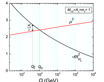
Figure 1: RGE evolutions of $\mu^{2}$ and $-m_{H_{u}}^{2}$ are plotted as functions of the scale $Q$(GeV). The Higgsino mass $\mu$ is chosen to make $Q_{0}=1$ TeV. The proper $Z$ boson mass is evaluated at the scale $Q_{\tilde{t}}$.

The interpretation of Eq.(15) is illustrated in Fig.1. In Fig.1, the SUSY breaking mass parameters in mSUGRA are made to be dimensionless unit since the RGE evolution does not depend on overall scale factor. As it is obvious from the figure, the little hierarchy is characterized by the smallness of the triangle. The little hierarchy problem can be rephrased in terms of the question why the size of the triangle is small. There are two ways to make the triangle small. The vertical tuning corresponds to the tuning of $\mu$ parameter with fixed $M_{H}$ as in the previous section. The $\mu$ parameter tuning is equivalent to tuning $Q_{0}$ after fixing $Q_{\tilde{t}}$. The horizontal adjustment of the triangle corresponds to the tuning of $\ln(Q_{0}/Q_{\tilde{t}})$.

We stress that the smallness of $\mu$ is not crucial for the little hierarchy due to the fact that $m_{H_{u}}^{2}$ and $\mu^{2}$ are canceled at $Q_{0}$. In that sense, the usual fine-tune quantity $\Delta[M_{Z}(\mu)]=M_{Z}^{2}/2\mu^{2}$ does not play a key role to describe fine-tuning in radiative electroweak symmetry breaking when $Q_{0}$ is fixed at a TeV scale. We point out that the horizontal adjusting quantity $\ln(Q_{0}/Q_{\tilde{t}})$ is more important to discuss the little hierarchy in radiative electroweak symmetry breaking. Actually, one can calculate the sensitivity function of $\Delta[M_{Z}(Q_{\tilde{t}})]$ to be

$$\Delta[M_{Z}(Q_{\tilde{t}})]\simeq\frac{\ln\left(\frac{Q_{0}}{Q_{\tilde{t}}}\right)^{\!2}}{\left|1-\ln\left(\frac{Q_{0}}{Q_{\tilde{t}}}\right)^{\!2}\right|}\,.$$ (19)

If $\ln(Q_{0}/Q_{\tilde{t}})\sim 0$, then $\Delta[M_{Z}(Q_{\tilde{t}})]$ is small and $Z$ boson mass is sensitive to $Q_{\tilde{t}}$.

The question is now whether $\ln(Q_{0}/Q_{\tilde{t}})^{2}\mathrel{\mathchoice{\lower 2.58334pt\vbox{\halign{$\m@th\displaystyle\hfil#\hfil$\cr<\crcr\sim\crcr}}}{\lower 2.58334pt\vbox{\halign{$\m@th\textstyle\hfil#\hfil$\cr<\crcr\sim\crcr}}}{\lower 2.58334pt\vbox{\halign{$\m@th\scriptstyle\hfil#\hfil$\cr<\crcr\sim\crcr}}}{\lower 2.58334pt\vbox{\halign{$\m@th\scriptscriptstyle\hfil#\hfil$\cr<\crcr\sim\crcr}}}}O(1)$ is natural. Apparently, there is no reason that $Q_{\tilde{t}}$ is related to $Q_{0}$. For example, let us assume that all the mass parameters (including $\mu$ and $B$) to be proportional to a single mass scale $M_{S}$. Namely, the mass parameters in the model are written as $m_{\tilde{Q}}^{2}=\hat{m}_{\tilde{Q}}^{2}M_{S}^{2}$, $m_{\tilde{g}}=\hat{m}_{\tilde{g}}M_{S}$, $A_{u}=\hat{A}_{u}M_{S}$, $\mu=\hat{\mu}M_{S}$ and so on. The dimensionless coefficients $\hat{m}_{\tilde{Q}}^{2}$, $\hat{m}_{\tilde{g}}$, $\hat{A}_{u}$ etc are determined when we fix a SUSY breaking scenario. The $\mu$ parameter is also proportional to SUSY breaking scale in Giudice-Masiero mechanism [13] in which the $\mu$-term is forbidden in the superpotential by a symmetry and the Higgsino mass originates from the Higgs bilinear term in Kähler potential. In this case, $Q_{0}$ does not depend on $M_{S}$ since RGEs are homogeneous differential equations. The averaged stop mass $Q_{\tilde{t}}$, on the other hand, of course depends on $M_{S}$. Since the scale $Q_{0}$ is determined radiatively, it is hierarchically smaller than the grand unified scale or the Planck scale $M_{P}$. Namely, the scale $Q_{\tilde{t}}$ is a dimensionful parameter, while the scale $Q_{0}$ is expressed as $Q_{0}\sim e^{-4\pi^{2}t}M_{P}$ by a dimensionless $O(1)$ parameter $t$. How can those two scales be related? Actually, in any SUSY breaking scenario, the determination of the coefficients and the overall scale are completely different issues. Why $Q_{0}$ and $Q_{\tilde{t}}$ are so close to make $\ln(Q_{0}/Q_{\tilde{t}})^{2}\mathrel{\mathchoice{\lower 2.58334pt\vbox{\halign{$\m@th\displaystyle\hfil#\hfil$\cr<\crcr\sim\crcr}}}{\lower 2.58334pt\vbox{\halign{$\m@th\textstyle\hfil#\hfil$\cr<\crcr\sim\crcr}}}{\lower 2.58334pt\vbox{\halign{$\m@th\scriptstyle\hfil#\hfil$\cr<\crcr\sim\crcr}}}{\lower 2.58334pt\vbox{\halign{$\m@th\scriptscriptstyle\hfil#\hfil$\cr<\crcr\sim\crcr}}}}O(1)$? This is an essential question of radiative electroweak symmetry breaking and the origin of SUSY breaking. In addition, when $Q_{0}<Q_{\tilde{t}}$, the electroweak symmetry does not break. It is just like living on the edge of a cliff.

4 Landscape of Electroweak Symmetry Breaking Vacua

Anthropic principle teaches us that we need not worry about the fact that $Q_{\tilde{t}}$ appears within the window for electroweak symmetry breaking, Eq.(12). So, the question is whether the little hierarchy is natural among the electroweak symmetry breaking vacua. To see that, we examine the landscape of the electroweak symmetry breaking vacua.

As we have mentioned in the previous section, let us assume that all mass parameters are proportional to single SUSY breaking mass scale such that $m_{\tilde{Q}}^{2}=\hat{m}_{\tilde{Q}}^{2}M_{S}^{2}$, $m_{\tilde{g}}=\hat{m}_{\tilde{g}}M_{S}$, $A_{u}=\hat{A}_{u}M_{S}$, $\mu=\hat{\mu}M_{S}$ and so on. Then, the radiative electroweak symmetry breaking scale $Q_{0}$ does not depend on $M_{S}$ when the dimensionless coefficients are fixed. On the other hand, $Q_{\tilde{t}}$ is naively proportional to $M_{S}$. The SUSY breaking mass scale $M_{S}$ is specified by the $F$-term of a SUSY breaking spurion field $X$, as $M_{S}\propto|F_{X}|/M_{P}$. If any complex value of $F_{X}$ is equally probable, the distribution function of $M_{S}$ is $D[M_{S}]\propto M_{S}$. Therefore, as one of the simplest example, we calculate the distribution function when the distribution of $Q_{\tilde{t}}$ is proportional to $Q_{\tilde{t}}$ after fixing $Q_{0}$.

Now, we calculate the distribution function of the $Z$ boson and the stop mass hierarchy using Eq.(18). The hierarchy $R_{\tilde{t}}\equiv M_{Z}/\bar{m}_{\tilde{t}}$ is given as

$$R_{\tilde{t}}^{2}=\alpha\ln\frac{Q_{0}}{Q_{\tilde{t}}}\,,$$ (20)

where $\bar{m}_{\tilde{t}}$ is an averaged stop mass, $\bar{m}_{\tilde{t}}^{2}=(m_{\tilde{t}_{L}}^{2}+m_{\tilde{t}_{R}}^{2})/2$ and $\alpha$ is the coefficient

$$\alpha\simeq\frac{3}{4\pi^{2}}\left(2+\left(\frac{A_{t}}{\bar{m}_{\tilde{t}}}\right)^{2}\right).$$ (21)

Using the relation, $D[R_{\tilde{t}}]=D[Q_{\tilde{t}}]dQ_{\tilde{t}}/dR_{\tilde{t}}$, we obtain the distribution function of $R_{\tilde{t}}$ as

$$D[R_{\tilde{t}}]=\frac{4}{\alpha}R_{\tilde{t}}\,\exp\left({-2\frac{R_{\tilde{t}}^{2}}{\alpha}}\right),$$ (22)

where we normalize the distribution function to make $\displaystyle\int_{0}^{\infty}D[R_{\tilde{t}}]dR_{\tilde{t}}=1$. When $Q_{\tilde{t}}\ll Q_{0}$, the stability condition will break, but we neglect the condition to calculate the distribution function since the distribution for $Q_{\tilde{t}}\ll Q_{0}$ ($R_{\tilde{t}}\gg 1$) is exponentially suppressed.

Figure 2: The distribution functions $D[R_{\tilde{t}}]$ (left) and $D[R^{2}_{\tilde{t}}]$ (right) are shown.

We plot the distribution function $D[R_{\tilde{t}}]$ in the case $A_{t}/{\bar{m}}_{\tilde{t}}=1$ (namely $\alpha=9/(4\pi^{2})$) in Fig.2. The peak of the distribution is $R_{\tilde{t}}=\sqrt{\alpha}/2\simeq 0.24.$ From the distribution, one can find that a little hierarchy between the stop and the $Z$ boson masses are probable among the electroweak symmetry breaking vacua. When we look at the distribution function of $R_{\tilde{t}}^{2}$ ($2R\cdot D[R^{2}]=D[R]$),

$$D[R^{2}_{\tilde{t}}]=\frac{2}{\alpha}\exp\left(-2\frac{R_{\tilde{t}}^{2}}{\alpha}\right),$$ (23)

it becomes more clear that there is a strong probability for $\ln Q_{0}/Q_{\tilde{t}}\simeq 0$.

Usually, it is said that a small value of $\Delta[f(x)]$ is unwanted since $f$ is sensitive for $x$ and a fine-tuning is needed. In fact, for the $\mu$ distribution in the section 2, the probability function naively corresponds to the sensitivity function. However, we have encountered an example where the probability and the sensitivity have different qualitative features. Namely, the fine-tuning becomes most probable.

One may think that it looks awkward that fine-tuning is preferable. However, it can happen when we consider a distribution. Let us illustrate it for the distribution of $f(x)=a\ln(1/x)$. Assume that any $x$ is equally probable for $0<x<1$. Then $y=f(x)$ is distributed for $y>0$ and the distribution function is obtained as $D[y]\propto\exp(-y/a)$. On the other hand, $\Delta[f(x)]=\ln(1/x)=y/a$. Therefore, $y\sim 0$ is the most probable, while the sensitivity function becomes zero at the point. It can be understood intuitively from the semi-log graph such as in the Fig.1. The vertical lines are dense for larger values of horizontal logarithmic axis. Surely, $y<0$ is more probable than $y>0$ if $x>1$ is allowed. However, if we compare this example with our model of concern, $y<0$ corresponds to the vacua where the electroweak symmetry breaking would not happen. Among the electroweak symmetry breaking vacua, therefore, the fine-tuned vacua are more probable. Furthermore, the distribution for less hierarchy is exponentially suppressed due to the loop factor $\alpha$.

As seen in the Fig.2, the shape of the distribution function looks different in different measures, $dR_{\tilde{t}}$ or $dR_{\tilde{t}}^{2}$. So it is better to use the probability function for a numerical quantity of little hierarchy instead of the distribution function. The probability for $R_{\tilde{t}}>R_{0}$ is given by

$$P[R_{\tilde{t}}>R_{0}]=\int_{R_{0}}^{\infty}D[R_{\tilde{t}}]dR_{\tilde{t}}=\exp\left(-2\frac{R_{0}^{2}}{\alpha}\right).$$ (24)

So, we obtain the probability for $\bar{m}_{\tilde{t}}>2M_{Z}\ (3M_{Z})$ is 89% (62%), and

$$\bar{m}_{\tilde{t}}<(830\ {\rm GeV})\ \sqrt{\frac{3}{2+(A_{t}/\bar{m}_{\tilde{t}})^{2}}}\,,$$ (25)

at 90% probability.

We have assumed that the distribution function of $M_{S}$ is proportional to $M_{S}$ because the SUSY breaking order parameter is complex. When the order parameter is real in the case of $D$-term breaking, the distribution function of $M_{S}$ is constant. In general, if $n$ real components cooperate the overall SUSY breaking scale, the distribution function is $D[M_{S}]\propto M_{S}^{n-1}$ (or $D[M_{S}^{n}]={\rm const}$), and we obtain the probability function as

$$P[R_{\tilde{t}}>R_{0}]=\exp\left(-n\frac{R_{0}^{2}}{\alpha}\right).$$ (26)

In Ref.[7], the authors use an average of $R_{\tilde{t}}^{2}$,

$$\langle R_{\tilde{t}}^{2}\rangle=\int_{0}^{\infty}R_{\tilde{t}}^{2}D[R_{\tilde{t}}]dR_{\tilde{t}}=\frac{\alpha}{n}\,,$$ (27)

to claim the closeness of the $Q_{\tilde{t}}$ and $Q_{0}$. The probability that it is more hierarchical than the average is 63% ($=1-1/e$), namely, it is about two times more probable rather than that of less hierarchy. Therefore, we propose to use the probability to describe the little hierarchy.

Since the sensitivity function is not the proper quantity in the landscape picture distributing the overall SUSY breaking scale, we suggest to use the probability function Eq.(26) to characterize the little hierarchy. We plot the 90% and 95% probability contours (in the case of $n=2$) in the minimal supergravity with $A_{0}=0$ and $\tan\beta=10,40$. To calculate the probability, we only distribute the overall SUSY breaking scale for each $m_{0}/m_{1/2}$ ratio.

As calculated in Eq.(25), the averaged stop mass is less than 1 TeV at 90% probability. We can see from the figure that the 95% probability region can be tested at the LHC and the future dark matter detection experiments since the SUSY particle masses are not very large. This region lies in the allowed parameter space. The parameter space is constrained by the dark matter constraint [14], the lower limit on Higgs mass, LEP bounds on SUSY particles [15], $b\rightarrow s\gamma$ bound [16] and the muon $g-2$ data [17].

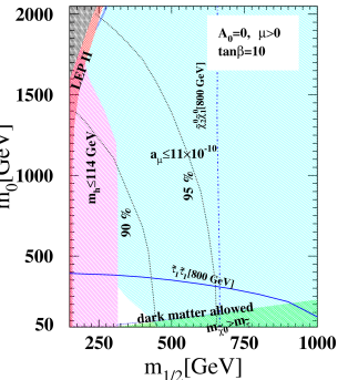
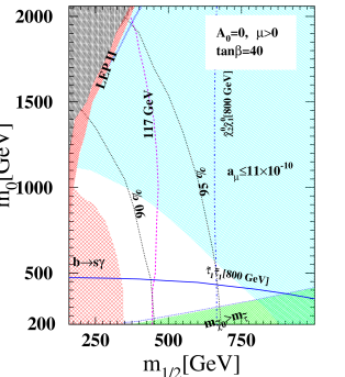
Figure 3: 90% and 95% probability contours (black lines) are shown in the allowed parameter space for $\tan\beta=10$ (left) and $\tan\beta=40$ (right). The blue narrow bands are allowed by dark matter constraints. The lightest Higgs mass $m_{H}\leq 114$ GeV is in the pink shaded region. The red shaded region is disallowed by the LEP data. The lightest supersymmetry particle is charged in the green region. $a_{\mu}\leq 11\times 10^{-10}$ in the light blue shaded region. The brick red hatched region obeys the $2.2\times 10^{-4}<{\rm Br}[b\rightarrow s\gamma]<4.5\times 10^{-4}$ constraint. The blue vertical and horizontal line show the ILC (800 GeV) reach in $\tilde{\chi}^{0}_{2}\tilde{\chi}^{0}_{1}$ and $\tilde{\tau}_{1}\tilde{\tau}_{1}$ final states. The black region is not allowed by radiative electroweak symmetry breaking. We use $m_{t}=172.7$ GeV for this graph.

5 Several Landscapes in Minimal Supergravity

In the minimal supergravity model [2, 3], the parameters are given as ($m_{0},m_{1/2},A_{0},\mu,B$). One usually uses $B$ to determine $\tan\beta$, and uses $\mu$ to solve $M_{Z}$ using Eq.(5) at the weak scale. So far, the parameter set is ($m_{0},m_{1/2},A_{0},\tan\beta,{\rm sgn}(\mu)$). In solving the equation for the $Z$ boson mass by $\mu$, one may need fine-tuning and the probability of fine-tuning is small as we have seen in section 2.

In the landscape, as we have seen in the previous section, the dimensionless parameters ($\hat{m}_{0}$, $\hat{A}_{0}$, $\hat{\mu}$, $\tan\beta$) are given and one dimensionful scale $m_{1/2}$ is distributed, where $\hat{m}_{0}=m_{0}/m_{1/2}$, $\hat{A_{0}}=A_{0}/m_{1/2}$, $\hat{\mu}=\mu/m_{1/2}$. The electroweak symmetry breaking scale $Q_{0}$ is the function of these four dimensionless parameters up to a cutoff scale, $M_{P}$ or $M_{\rm GUT}$. Once these four parameters are fixed, $m_{1/2}$ is consumed to solve $Z$ boson mass and a fine-tuning may be needed. However, the fine-tuning for the little hierarchy has enough probability among the landscape of electroweak symmetry breaking vacua.

The difference in above two results depends on what parameter is distributed in the landscape. In the first case, ($m_{0}$, $A_{0}$, $m_{1/2}$, $\tan\beta$) is fixed and $\mu$ is distributed, and in the latter case, ($\hat{m}_{0}$, $\hat{A}_{0}$, $\hat{\mu}$, $\tan\beta$) is fixed and $m_{1/2}$ is distributed. In the landscape distributed by $\mu$, the fine-tuning vacua is less probable, and thus the small $\mu$ is demanded as in the usual naturalness statement. We emphasize that the usual naturalness statement is not necessarily applied in the landscape distributed by $m_{1/2}$.

In the anthropic picture, the landscape mostly prefers a little hierarchy irrespective of $Q_{0}$. We are interested in the vacua where $Q_{0}$ is at TeV scale in our universe. In the parameter space where $Q_{0}$ is at TeV scale, $\hat{\mu}$ is not necessarily small. Actually, $\hat{\mu}$ is almost determined irrespective of $\hat{m}_{0}$ when $Q_{0}$ is at a TeV scale in the minimal supergravity since $M_{H}^{2}$ has a focus point around the TeV scale [18]. As a result, the $\mu$ parameter and the CP odd Higgs boson mass can be large with enough probability in the landscape contrary to the usual naturalness statement.

We have fixed the scale $Q_{0}$ in our discussion of landscape in the previous section. What happens when $Q_{0}$ is also distributed? To see that, let us study the distribution of $Q_{0}$ as well as the other parameters.

5.1 Landscape of the scale $Q_{0}$

Let us first see the landscape of the scale $Q_{0}$ distributed by $\mu$. The scale is given as

$$\mu^{2}(Q_{0})=M_{H}^{2}(Q_{0})\simeq-m_{H_{u}}^{2}(Q_{0}).$$ (28)

The scale dependence of $\mu$ can be written as $\mu^{2}(Q_{0})=\mu_{0}^{2}I(Q_{0})$. Therefore, when any complex value of $\mu_{0}$ is equally probable ($D[|\mu_{0}|^{2}]={\rm const}$), the distribution of $t_{0}\equiv\ln Q_{0}$ is

$$D[t_{0}]=D[\mu^{2}_{0}]\frac{d\mu_{0}^{2}}{dt_{0}}=c\,\frac{d}{dt_{0}}\frac{{M}_{H}^{2}(t_{0})}{I(t_{0})},$$ (29)

where $c$ is a constant. The $\mu$ parameter may be a function of moduli, e.g. $\mu=f(z)$. Then the $\mu$ distribution is $D[\mu]=D[z]df^{-1}/d\mu$. In the case where $D[\mu^{m}_{0}]={\rm const}$, we obtain

$$D[t_{0}]=c\left(\frac{M_{H}^{2}}{I}\right)^{\frac{m-2}{2}}\frac{d}{dt_{0}}\frac{M_{H}^{2}}{I}.$$ (30)

The maximal value of $Q_{0}$ is the scale where $M_{H}^{2}=0$. We define this scale $Q_{H}$, namely $M_{H}^{2}(Q_{H})=0$. Surely, $Q_{H}$ does not depend on $\mu$ and the overall mass scale. Since the RGE of $m^{2}_{H_{u}}$ becomes larger at lower scale, the large $Q_{0}$-$Q_{H}$ hierarchy ($Q_{0}\ll Q_{H}$) is more probable for $m\geq 2$. However, the little hierarchy between $Z$ boson mass and SUSY breaking masses is not very probable as we have seen in section 2.

5.2 Landscape of the scale $Q_{H}$

How about the $Q_{H}$ landscape? The scale $Q_{H}$ is function of $\hat{m}_{0}$, $\hat{A}_{0}$ (in the unit of $m_{1/2}$) and $\tan\beta$. For simplicity, let us choose $A_{0}=0$ and neglect $\tan\beta$ dependence. We parameterize $\hat{m}_{0}=\tan\theta_{T}$ and any $\theta_{T}$ ($0<\theta_{T}<\pi/2$) is equally probable. The $\theta_{T}$ can be identified to the mixing between dilaton and moduli which breaks SUSY. The scale dependence of $m_{H_{u}}^{2}$ can be written as

$$m_{H_{u}}^{2}(Q)=m_{0}^{2}K_{0}(Q)+m_{1/2}^{2}K_{1/2}(Q).$$ (31)

Then the distribution function of the scale $t_{H}\equiv\ln Q_{H}$ where $m_{H_{u}}(Q_{H})=0$ is

$$D[t_{H}]=c\,\sqrt{\frac{K_{0}}{K_{1/2}}}\frac{K_{0}}{K_{0}+K_{1/2}}\frac{d}{dt}\frac{K_{1/2}}{K_{0}}.$$ (32)

In the minimal supergravity, $Q_{H}$ has a maximal value $Q_{H}^{\rm max}\sim 10^{10}$ GeV for $\hat{m}_{0}=0$ and $K_{1/2}(Q_{H}^{\rm max})=0$, and a minimal value $Q_{H}^{\rm min}\sim 5$ TeV (when $\tan\beta=40$) for large $\hat{m}_{0}$ and $K_{0}(Q_{H}^{\rm min})=0$. We plot the distribution function in Fig.4. The scale $t_{H}$ does not have strong preference except for the scales to be around the minimal and maximal values. The probability around the minimal and maximal values arising from the integration of the distribution function is not very large. Therefore, in the landscape, we do not obtain a typical preference of the hierarchy.

Figure 4: The distribution of $Q_{H}$ is shown when $\hat{m}_{0}=m_{0}/m_{1/2}$ is distributed. $Q_{H}$ is the scale where SUSY breaking Higgs mass squared becomes negative.

5.3 Landscapes of $Q_{\tilde{t}}$ and $Q_{0}$

We distribute both $m_{1/2}$ and $\hat{\mu}$ with $D[m_{1/2}^{2}]=D[\hat{\mu}^{2}]={\rm const}$. The distribution function is given as $dP=D[m_{1/2}^{2}]D[\hat{\mu}^{2}]dm_{1/2}^{2}d\hat{\mu}^{2}$. We note that $d\mu$ and $d\hat{\mu}$ is the same measure up to normalization when $m_{1/2}$ is fixed, but if $m_{1/2}$ is also distributed, those two measures need to be distinguished.

When $m_{1/2}$ and $\hat{\mu}$ are distributed, both $Q_{\tilde{t}}$ and $Q_{0}$ are distributed. The distribution function of $t_{0}$ and $\tilde{t}\equiv\ln Q_{\tilde{t}}$ can be written as $D[t_{0},\tilde{t}]=c\,\theta(t_{0}-\tilde{t})\,e^{2\tilde{t}}\frac{d}{dt}\frac{M_{H}^{2}}{I}|_{t=t_{0}}$, where $\theta$ is a step function. Defining $t_{Z}\equiv t_{0}-\tilde{t}$ ($t_{Z}>0$), we obtain

$$D[t_{0},t_{Z}]=c\,e^{-2t_{Z}}e^{2t_{0}}\left.\frac{d}{dt}\frac{M_{H}^{2}}{I}\right|_{t=t_{0}},$$ (33)

and the distribution function can be decomposed as $D[t_{Z}]\propto e^{-2t_{Z}}$ and $D[t_{0}]\propto e^{2t_{0}}|\frac{d}{dt}M_{H}^{2}/I|$. The hierarchy between the $Z$ boson and stop mass is given as $M_{Z}^{2}/\bar{m}_{\tilde{t}}=\alpha t_{Z}$ as in Eq.(20). The little hierarchy of $M_{Z}$-$\bar{m}_{\tilde{t}}$ is probable from the distribution function $D[t_{Z}]\propto e^{-2t_{Z}}$ in the same way when we just use $m_{1/2}$ distribution.

Since the large $t_{0}$ is strongly probable due to the exponential factor in the distribution function $D[t_{0}]\propto e^{2t_{0}}|\frac{d}{dt}M_{H}^{2}/I|$, the scale $Q_{0}$ is most probably just below the maximal value of $Q_{0}$ which is the scale $Q_{H}$. Therefore, all three scales, $Q_{\tilde{t}}$, $Q_{0}$ and $Q_{H}$ are close by. Since $Q_{0}$ is just below the scale $Q_{H}$, the $\mu$ parameter must be small by definition:

$$\mu^{2}(Q_{0})\simeq\ln\frac{Q_{0}}{Q_{H}}\frac{d}{dt}M_{H}^{2}.$$ (34)

In fact, the small $\mu$ is the most probable as one can see from the distribution function which is calculated as

$$D[\mu^{2}(Q_{0})]\simeq c\left(1+\frac{\dot{\mu}^{2}}{|\dot{M}_{H}^{2}|}\right)\exp\left(-2\frac{\mu^{2}}{|\dot{M}_{H}^{2}|}\right),$$ (35)

where dot represents for $t=\ln Q$ derivative. Therefore, this landscape mostly prefers the little hierarchy with small Higgsino mass, which is a demand from naturalness. For our universe, we have to choose the SUSY breaking scenario to make the $Q_{H}$ to be TeV scale. In the minimal supergravity, $\hat{m}_{0}$ needs to be large to make $Q_{H}$ to be at the TeV scale, which corresponds to the focus point solution [18]. We stress that naturalness is not required in this landscape, but the naturalness vacua are most probable.

We remark that $Q_{H}$ must not be distributed in this landscape, otherwise SUSY breaking scale becomes just below the maximal value of $Q_{H}$, which is $10^{10}$ GeV in minimal supergravity.

5.4 Summary of different Landscapes

We have studied several landscapes to distribute parameters ($m_{1/2}$, $\hat{\mu}$, $\hat{m}_{0}$) in minimal supergravity. The important scales to describe the landscape of electroweak symmetry breaking vacua are stop mass $Q_{\tilde{t}}$, symmetry breaking scale $Q_{0}$ (at $\mu^{2}=M_{H}^{2}$), and the scale $Q_{H}$ where $M_{H}=0$. The scales $Q_{0}$ and $Q_{H}$ do not depend on the overall mass scale which we choose $m_{1/2}$, and $Q_{H}$ does not depend on $\hat{\mu}$.

We consider the following typical landscapes:

1. If we distribute the overall mass scale that is chosen to be $m_{1/2}$, we can obtain a little hierarchy with enough probability irrespective of the sensitivity function. Naturalness (smallness of $\mu$) is not necessary in the landscape.

2. If we distribute $\mu$ and fix the overall scale, the little hierarchy between $Z$ boson mass and SUSY breaking scale is not probable, but the hierarchy between $Q_{0}$-$Q_{H}$ is probable i.e., a large $\mu$ could exist.

3. If we distribute only $\hat{m}_{0}$, we do not obtain any particular probable hierarchy.

4. If we distribute both $m_{1/2}$ and $\hat{\mu}$, it is probable that all three scales are close. Therefore, naturalness vacua with little hierarchy is the most probable. The SUSY breaking scenario needs to be fixed to make $Q_{H}$ (or $Q_{H}^{\rm max}$ if it is distributed) to be TeV scale in our universe. In the mSUGRA model, $\hat{m}_{0}\simeq O(10)$ is required. One can consider specific SUSY breaking models such as in Ref.[19, 20].

6 Conclusion

The absence of the SUSY signals at LEP and Tevatron has pushed up the SUSY particle mass scale compared to the $M_{Z}$ scale. The colored SUSY particles are now around 1 TeV scale in the mSUGRA models and therefore created a little hierarchy between this scale and the $Z$ boson mass scale. It is said that naturalness of the electroweak symmetry breaking requires the smallness of the Higgsino mass $\mu$.

We investigated this situation in the context of landscape of electroweak symmetry breaking vacua. We include radiative symmetry breaking and found that in order to obtain a little hierarchy between $Z$ boson mass and SUSY breaking scale with enough probability, we need to distribute the overall SUSY breaking mass scale. In this landscape, the naturalness (small value of $\mu$) is not required. The Higgsino mass $\mu$ can be large or small and the scale $Q_{0}$ where the electroweak symmetry breaking conditions are satisfied needs to be chosen around 1 TeV in our universe as one of the vacua in the landscape of little hierarchy. In this scenario, the SUSY breaking mass is preferred to be just below the scale $Q_{0}$, in the electroweak symmetry breaking vacua and therefore the little hierarchy can be rationalized.

If $\mu$ is also distributed along with the overall SUSY breaking mass, natural vacua (small $\mu$) is found to be probable among the electroweak symmetry breaking vacua. In this landscape, the scale $Q_{H}$, where the SUSY breaking Higgs mass squared turns negative, has to be selected at a TeV scale in our universe by choosing a SUSY breaking scenario.

If we only distribute $\mu$, the little hierarchy is less probable, and the naturalness is demanded as usually discussed.

We note that the landscape with overall scale distribution supports the little hierarchy with enough probability, but do not support huge hierarchy between SUSY breaking scale and the $Z$ boson mass, such as split SUSY [21] or non-SUSY standard model at low energy where all SUSY particles are decoupled. Actually, the stop mass is less than 3 TeV at 99% probability. We also comment that the vacua with all scalar particles (including Higgs fields) and gauginos being decoupled are enormously probable rather than low energy SUSY vacua in this landscape picture. The proper statement is that the little hierarchy is mostly probable among the low energy SUSY vacua with radiative electroweak symmetry breaking by Higgs mechanism.

References

- [1] S. Dimopoulos and H. Georgi, Nucl. Phys. B 193, 150 (1981); S. Dimopoulos, S. Raby and F. Wilczek, Phys. Rev. D 24, 1681 (1981); N. Sakai, Z. Phys. C 11, 153 (1981); L. E. Ibanez and G. G. Ross, Phys. Lett. B 105, 439 (1981); M. B. Einhorn and D. R. T. Jones, Nucl. Phys. B 196, 475 (1982); W. J. Marciano and G. Senjanovic, Phys. Rev. D 25, 3092 (1982).
- [2] D. Z. Freedman, P. van Nieuwenhuizen and S. Ferrara, Phys. Rev. D 13, 3214 (1976); S. Deser and B. Zumino, Phys. Lett. B 62, 335 (1976); A. H. Chamseddine, R. Arnowitt and P. Nath, Phys. Rev. Lett. 49, 970 (1982).
- [3] R. Barbieri, S. Ferrara and C. A. Savoy, Phys. Lett. B 119, 343 (1982); L. J. Hall, J. D. Lykken and S. Weinberg, Phys. Rev. D 27, 2359 (1983); P. Nath, R. Arnowitt and A. H. Chamseddine, Nucl. Phys. B 227, 121 (1983); For a review, see P. Nilles, H. P. Nilles, Phys. Rept. 110, 1 (1984).
- [4] J. R. Ellis, K. Enqvist, D. V. Nanopoulos and F. Zwirner, Mod. Phys. Lett. A 1, 57 (1986); R. Barbieri and G. F. Giudice, Nucl. Phys. B 306, 63 (1988); G. W. Anderson and D. J. Castano, Phys. Lett. B 347, 300 (1995) [hep-ph/9409419]; K. L. Chan, U. Chattopadhyay and P. Nath, Phys. Rev. D 58, 096004 (1998) [hep-ph/9710473].
- [5] L. Susskind, hep-th/0302219; M. R. Douglas, JHEP 0305, 046 (2003) [hep-th/0303194]; F. Denef and M. R. Douglas, JHEP 0405, 072 (2004) [hep-th/0404116].
- [6] K. Inoue, A. Kakuto, H. Komatsu and S. Takeshita, Prog. Theor. Phys. 68, 927 (1982) [Erratum-ibid. 70, 330 (1983)]; Prog. Theor. Phys. 71, 413 (1984); L. E. Ibanez and G. G. Ross, Phys. Lett. B 110, 215 (1982); L. E. Ibanez, Phys. Lett. B 118, 73 (1982); Nucl. Phys. B 218, 514 (1983); L. Alvarez-Gaume, J. Polchinski and M. B. Wise, Nucl. Phys. B 221, 495 (1983); J. R. Ellis, J. S. Hagelin, D. V. Nanopoulos and K. Tamvakis, Phys. Lett. B 125, 275 (1983).
- [7] G. F. Giudice and R. Rattazzi, Nucl. Phys. B 757, 19 (2006) [hep-ph/0606105].
- [8] K. Choi, K. S. Jeong and K. i. Okumura, JHEP 0509, 039 (2005) [hep-ph/0504037]; K. Choi, K. S. Jeong, T. Kobayashi and K. i. Okumura, Phys. Lett. B 633, 355 (2006) [hep-ph/0508029]; hep-ph/0612258.
- [9] R. Kitano and Y. Nomura, Phys. Lett. B 631, 58 (2005) [hep-ph/0509039]; Phys. Lett. B 632, 162 (2006) [hep-ph/0509221]; Phys. Rev. D 73, 095004 (2006) [hep-ph/0602096]; hep-ph/0606134.
- [10] S. R. Coleman and E. Weinberg, Phys. Rev. D 7, 1888 (1973).
- [11] J. A. Casas, V. Di Clemente and M. Quiros, Nucl. Phys. B 553, 511 (1999) [hep-ph/9809275]; D. V. Gioutsos, Eur. Phys. J. C 17, 675 (2000) [hep-ph/9905278].
- [12] J. R. Ellis, A. B. Lahanas, D. V. Nanopoulos and K. Tamvakis, Phys. Lett. B 134, 429 (1984); J. R. Ellis, C. Kounnas and D. V. Nanopoulos, Phys. Lett. B 143, 410 (1984).
- [13] G. F. Giudice and A. Masiero, Phys. Lett. B 206, 480 (1988).
- [14] D. N. Spergel et al. [WMAP Collaboration], Astrophys. J. Suppl. 148, 175 (2003) [astro-ph/0302209].
- [15] R. Barate et al. [LEP Working Group for Higgs boson searches], Phys. Lett. B 565, 61 (2003) [hep-ex/0306033]; W. M. Yao et al. [Particle Data Group], J. Phys. G 33, 1 (2006).
- [16] M. S. Alam et al. [CLEO Collaboration], Phys. Rev. Lett. 74, 2885 (1995).
- [17] G. W. Bennett et al. [Muon Collaboration], Phys. Rev. Lett. 92, 161802 (2004) [hep-ex/0401008]; S. Eidelman, Talk at ICHEP 2006, Moscow, Russia.
- [18] K. L. Chan, U. Chattopadhyay and P. Nath, Phys. Rev. D 58, 096004 (1998) [hep-ph/9710473]. J. L. Feng, K. T. Matchev and T. Moroi, Phys. Rev. Lett. 84, 2322 (2000) [hep-ph/9908309]; Phys. Rev. D 61, 075005 (2000) [hep-ph/9909334].
- [19] Y. Nomura and D. Poland, hep-ph/0611249.
- [20] R. Dermisek and H. D. Kim, Phys. Rev. Lett. 96, 211803 (2006) [hep-ph/0601036].
- [21] N. Arkani-Hamed and S. Dimopoulos, JHEP 0506, 073 (2005) [hep-th/0405159]; G. F. Giudice and A. Romanino, Nucl. Phys. B 699, 65 (2004) [hep-ph/0406088].