Determination of the Neutrino Mass Hierarchy via the Phase of the Disappearance Oscillation Probability with a Monochromatic $\bar{\nu}_{e}$ Source.

Abstract

The neutrino mass hierarchy can be determined, in principle, by measuring a phase in the disappearance oscillation probability in vacuum, without relying on the matter effect, using a single channel. This phase is not the same for the normal and inverted neutrino mass spectra. In this paper, we give a complete description and physics understanding of the method. The key feature of the method is to detect advancement (normal) or retardation (inverted) of the phase of the atmospheric-scale oscillation relative to the solar-scale oscillation. We then show that this method can be realized with the recently proposed resonant $\bar{\nu}_{e}$ absorption reaction enhanced by Mössbauer effect. The unique feature of this setup is the ultra-monochromaticity of the observed $\bar{\nu}_{e}$’s. Because of this feature the phase advancement or retardation of atmospheric-scale neutrino oscillation is detectable after 20 or more oscillations if the source and the target are made sufficiently compact in size. A quantitative estimate of the sensitivity to mass hierarchy resolution is given. We have also examined how a possible continuation of such experiment can be carried out in order also to achieve high precision (few %) determination of the solar-scale oscillation parameters $\Delta m^{2}_{21}$ and $\theta_{12}$.

I Introduction

Among the remaining unknowns in neutrino physics, resolving the neutrino mass hierarchy may be one of the key importance to our understanding of physics of neutrino masses and the lepton flavor mixing review . Given the significance of the problem, it is natural that many methods are proposed for determining the mass hierarchy. The most conventional one would be to do neutrino and antineutrino comparison in long-baseline (LBL) accelerator based oscillation experiments LBL_matter1 ; LBL_matter2 . Because of the difference in how the matter effect interferes with the vacuum oscillation effect it can signal the sign of $\Delta m^{2}_{31}$, and hence the mass hierarchy. Other less conventional ideas include the methods using atmospheric neutrinos atm-method , $\nu_{e}$ and $\nu_{\mu}$ disappearance channels GJK ; NPZ ; MNPZ , supernova neutrinos SN-method1 ; SN-method2 , and neutrino-less double beta decay double-beta . These lists of references cannot be complete, and some of the other relevant references are quoted therein.

In this paper, we discuss yet another way of determining the neutrino mass hierarchy by a neutrino oscillation disappearance experiment using a single neutrino flavor in vacuum whereas in previous works NPZ ; MNPZ the method required the use of two different disappearance channels close to the first oscillation maximum. The possibility that the neutrino survival probability in vacuum can be sensitive to the neutrino mass hierarchy was first suggested in petcov using reactor neutrinos in the context of high-$\Delta m^{2}$ large mixing angle (LMA) solar neutrino solution. It was also pursued recently in the Hanohano project using a Fourier transform technique hanohano . We present here a complete formulation and physics understanding of the new method to determine the neutrino mass hierarchy.

This method utilizes the feature that the atmospheric-$\Delta m^{2}$ scale oscillation “interferes” with the solar-$\Delta m^{2}$ scale oscillation in a different way depending upon the mass hierarchy. We first carefully re-formulate the difference as an advancement or retardation of the phase of the atmospheric-scale neutrino oscillation relative to the solar-scale oscillation; For the $\nu_{e}$ and $\bar{\nu}_{e}$ disappearance probabilities, the atmospheric oscillation is continuously advanced (retarded) for the normal (inverted) hierarchy. Since the core of the problem exists in extracting long wavelength solar oscillation out of the two short wavelength atmospheric scale oscillations due to $\Delta m^{2}_{32}$ and $\Delta m^{2}_{31}$, it is the critical matter to identify which quantity to be held fixed in defining the mass hierarchy reversal from the normal to the inverted, or vice versa. To our understanding, the only known appropriate quantity to hold is the effective neutrino mass squared difference $\Delta m^{2}_{\text{ee}}$ (see Eq.(4)), the one which is actually observed in $\nu_{e}$ (or $\bar{\nu}_{e}$) disappearance measurement at the first few oscillation maxima and/or minima NPZ . We find it important to have the proper formalism because otherwise the sensitivity to the mass hierarchy resolution can be significantly overestimated.

Then, we point out that an experiment using the resonant $\bar{\nu}_{e}$ absorption reaction mikaelyan enhanced by Mössbauer effect recently proposed by Raghavan Raghavan gives the first concrete realization of the idea. (See early for earlier proposals of Mössbauer enhanced experiments.) Because of the monochromaticity of the $\bar{\nu}_{e}$ beam from the bound state beta decay bahcall , the phase advancement or retardation of atmospheric-scale neutrino oscillation is detectable after 20 or more oscillations if the source and the target are made sufficiently compact in size. The unique feature of this method is the use of this ultra-monochromatic neutrino source thereby sidestepping the very high energy resolution requirement requested with reactor or accelerator neutrinos.

A concrete plan for the experiment may be as follows; In the first stage the atmospheric $\Delta m^{2}_{\text{ee}}$ must be accurately measured in a way described in mina-uchi by a measurement at $\sim$10 m baseline. As we will see, the precision of the measurement must reach sub-percent level in order for this method to work. Then, in the second stage relative phase advancement or retardation of the atmospheric-scale neutrino oscillation must be detected by moving the detector to $\sim$350 m, this is just beyond the solar-scale oscillation distance for 18.6 keV neutrinos. Based on this plan we give a detailed estimate of the sensitivity to the resolution of the mass hierarchy.

Upon finishing the above measurement, it is natural to think about the continuation of the experiment by moving the detector to distances tuned for precision measurement of the oscillation parameters relevant for solar neutrinos, $\Delta m^{2}_{21}$ and $\theta_{12}$. We also give a detailed estimate of the accuracy for the determination of these parameters. It is notable that a resonant $\bar{\nu}_{e}$ absorption experiment could allow to make precise measurements of all mixing parameters that appear in the $\nu_{e}\to\nu_{e}$ oscillation channel: $\theta_{13}$, $\theta_{12}$, $\Delta m^{2}_{21}$, the effective atmospheric $\Delta m^{2}_{\rm ee}$ and the neutrino mass hierarchy.

In Sec. II, we first describe the essence of the method in an explanatory way. We then define our theoretical machinery using the effective $\Delta m^{2}_{\text{ee}}$. We also clarify the basic requirement for the measurement. In Sec. III, we discuss the concrete set up of the experiment and describe our statistical method for the analysis. We then give the analysis results on sensitivity to the mass hierarchy resolution. In Sec. IV, we describe the analysis for the determination of the solar oscillation parameters. In Sec. V, we finish by giving our concluding remarks. In Appendix  A, we give a different interpretation of the phenomena in terms of the effective mass squared differences whereas in Appendix B, we discuss how this method can be applied to the $\nu_{\mu}$ disappearance channel. This possibility has been discussed in gouvea-winter however the baseline required is $L\simeq 11000\left(E/0.6\text{ GeV}\right)$ km.

II How can $\nu_{e}$ disappearance measurement alone signal the neutrino mass hierarchy?

The vacuum $\nu_{e}$ survival probability using $\Delta_{ij}\equiv\Delta m^{2}_{ij}L/4E$ ($\Delta m^{2}_{ij}\equiv m^{2}_{i}-m^{2}_{j}$) as shorthand for the kinematical phase, can be written without any approximation as

$$P(\nu_{e}\rightarrow\nu_{e}) = 1-4|U_{e3}|^{2}|U_{e1}|^{2}\sin^{2}\Delta_{31}-4|U_{e3}|^{2}|U_{e2}|^{2}\sin^{2}\Delta_{32}-P_{\odot},$$ (1)

$$= 1-\frac{1}{2}\sin^{2}2\theta_{13}\left[1-\left(c^{2}_{12}\cos 2\Delta_{31}+s^{2}_{12}\cos 2\Delta_{32}\right)\right]-P_{\odot},$$

where the usual parameterization of the mixing matrix PDG is used with the abbreviations $c_{ij}\equiv\cos\theta_{ij}$ and $s_{ij}\equiv\sin\theta_{ij}$. Here $E$ is the neutrino energy and $L$ is the baseline distance. $P_{\odot}$, as defined by,

$$P_{\odot}\equiv 4|U_{e2}|^{2}|U_{e1}|^{2}\sin^{2}\Delta_{21}=\sin^{2}2\theta_{12}c^{4}_{13}\sin^{2}\Delta_{21},$$ (2)

is the oscillation probability associated with the solar $\Delta m^{2}$ scale. In this paper, we assume the standard three neutrino framework with CPT conservation (except for where we discuss possible CPT violation), which implies that Eq. (1) is also valid for $\bar{\nu}_{e}$.

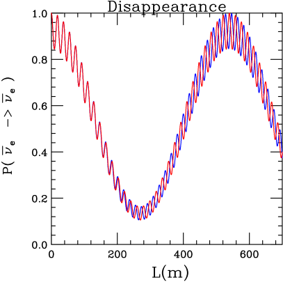
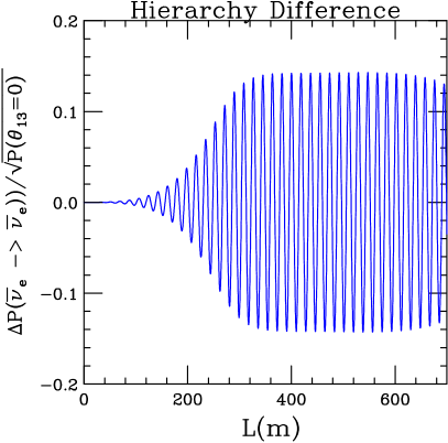
Figure 1: In the left panel, antineutrino survival probability $P(\bar{\nu}_{e}\rightarrow\bar{\nu}_{e})$ is plotted as a function of $L$. The blue and the red curves are for the normal and the inverted mass hierarchies, respectively. In the right panel, $\Delta P/\sqrt{P(\theta_{13}=0)}$, which is defined in the text, is shown. Here the neutrino energy was fixed to 18.6 keV. This choice comes from the experiment we will discuss later in this paper.

The neutrino mass hierarchy can be determined if one knows which kinematical phase, $|\Delta_{31}|$ or $|\Delta_{32}|$, is larger. Namely, if $|\Delta_{31}|>|\Delta_{32}|$ the normal hierarchy is the case, and if $|\Delta_{31}|<|\Delta_{32}|$ the inverted one. How we can know which is larger? When two waves with slight different frequencies travel together there arises the phenomenon of beating. The amplitude of superposed waves beats with the frequency corresponding to the difference of two frequencies. For $\nu_{e}$ disappearance probability, Eq. (1), we have beating because the frequency of the two waves in (1) with $|\Delta_{31}|$ and $|\Delta_{32}|$ differ by the frequency associated with the $|\Delta_{21}|$ characterized by the solar $\Delta m^{2}_{21}$ scale, which is smaller by a factor of $\simeq 30$ compared to the atmospheric $|\Delta_{31}|$ scale. One can decompose the superposed waves into the beating low frequency wave and the high frequency wiggles within the beat. Here, unlike the case addressed in most textbooks of basic physics, the amplitude of the two frequencies is different. Therefore, to tell which of the high frequencies has a larger amplitude, one has to determine whether the phase of the high frequency wiggles advances or retards as the wave evolves. This phase advancement or retardation can tell us whether the neutrino mass hierarchy is normal or inverted using only the disappearance measurement in a single channel, $\nu_{e}\rightarrow\nu_{e}$ in vacuum.

To demonstrate that it is possible, we plot in the left panel of Fig. 1 the oscillation probability $P(\nu_{e}\rightarrow\nu_{e})$ as a function of the distance $L$ from a source. As one can clearly see in the figure, the case of normal hierarchy ($\Delta m^{2}_{31}>0$, blue curve) starts to be distinguished from the case of inverted hierarchy ($\Delta m^{2}_{31}<0$, red curve) at around $L\sim 300$ m because of the advancement of the normal hierarchy’s high frequency wiggles and the retardation of the inverted hierarchy’s high frequency wiggles, i.e. the phase of the high frequency wiggles. What we mean by “beating” may be clearer in the left panel of Fig. 3 where the solar term is switched off.

To see the difference between the oscillation probabilities of the normal and the inverted hierarchies more clearly, we define the quantity

$$\Delta P(\nu_{e}\rightarrow\nu_{e}) \equiv P(\nu_{e}\rightarrow\nu_{e};\Delta m^{2}_{31}>0)-P(\nu_{e}\rightarrow\nu_{e};\Delta m^{2}_{31}<0).$$ (3)

Where the hierarchy flip is defined so that $|\Delta P|$ is minimized for short baseline measurements. (See Sec. II.1 for the precise definition of the hierarchy flip.) We normalize $\Delta P$ by dividing by $\sqrt{P(\theta_{13}=0)}$ since $P(\theta_{13}=0)$ is the “background” for seeing $\theta_{13}$ effects in $\nu_{e}$ disappearance. The quantity $\Delta P/\sqrt{P(\theta_{13}=0)}$ is plotted in the right panel of Fig. 1. The envelope of $|\Delta P|/\sqrt{P(\theta_{13}=0)}$ slowly rises from 0 to a plateau value of $\sin^{2}2\theta_{13}$ at a distance about 25% further from the source than the first solar oscillation maximum ($\Delta_{21}=\pi/2$ occurs when $L=280$ m) and remains reasonably constant at this value beyond the first solar oscillation minimum ($\Delta_{21}=\pi$). Clearly, even though the difference between the hierarchies is very small at short distances it becomes as large as theoretically possible, $\sin^{2}2\theta_{13}$ (see below), at large distances.

II.1 Theoretical framework

To decompose the superposed waves into the beat and wiggle, one has to correctly define the high frequency mode. We choose to do this by defining a short distance effective $\Delta m^{2}$ in the $\nu_{e}$ disappearance channel, see NPZ . It is given by

$$\Delta m^{2}_{\text{ee}}\equiv\cos^{2}\theta_{12}|\Delta m^{2}_{31}|+\sin^{2}\theta_{12}|\Delta m^{2}_{32}|.$$ (4)

This is the only linear combination of $\Delta m^{2}_{31}$ and $\Delta m^{2}_{32}$ that can be determined by a short distance (over the first few atmospheric oscillations) $\nu_{e}$ disappearance experiment. $\Delta m^{2}_{\text{ee}}$ is defined to be positive for both hierarchies. The choice of the atmospheric $\Delta m^{2}$ is crucial; Extraction of the low frequency mode can be done correctly only if the high frequency mode is identified in an appropriate way. See Sec. II.3 for more about it.

Now, we rewrite $P(\nu_{e}\rightarrow\nu_{e})$ without any approximation, using the positive and measurable variables $\Delta_{\text{ee}}\equiv\Delta m^{2}_{\text{ee}}L/4E$ and $\Delta_{21}$ and the phase $\phi_{\odot}$ (which will be given below), as follows:

$$P(\nu_{e}\rightarrow\nu_{e}) = 1-\frac{1}{2}\sin^{2}2\theta_{13}\left[1-\sqrt{1-\sin^{2}2\theta_{12}\sin^{2}\Delta_{21}}~{}\cos(2\Delta_{\text{ee}}\pm\phi_{\odot})\right]-P_{\odot},$$ (5)

where the positive (negative) sign in front of the phase $\phi_{\odot}$ corresponds to the normal (inverted) mass hierarchy; If $\Delta m^{2}_{\text{ee}}$ is precisely determined, the only effect of the hierarchy manifest itself as this sign. Clearly, the amplitude of the $\sin^{2}2\theta_{13}$ oscillations is modulated by $\sqrt{1-\sin^{2}2\theta_{12}\sin^{2}\Delta_{21}}$ which varies from 1 to $\cos 2\theta_{12}$ as the solar kinematic phase, $\Delta_{21}$, changes from $0\,(\text{mod}\,\pi)$ to $\pi/2\,(\text{mod}\,\pi)$. This amplitude modulation is the beat discussed in the previous section.

The phase $\phi_{\odot}$ in Eq. (5) depends only on solar parameters, $\Delta_{21}$ and $\theta_{12}$, and given as,

$$\sin\phi_{\odot} = \frac{c^{2}_{12}~{}\sin(2s^{2}_{12}\Delta_{21})-s^{2}_{12}~{}\sin(2c^{2}_{12}\Delta_{21})}{\sqrt{1-\sin^{2}2\theta_{12}\sin^{2}\Delta_{21}}},$$

$$\cos\phi_{\odot} = \frac{c^{2}_{12}~{}\cos(2s^{2}_{12}\Delta_{21})+s^{2}_{12}~{}\cos(2c^{2}_{12}\Delta_{21})}{\sqrt{1-\sin^{2}2\theta_{12}\sin^{2}\Delta_{21}}}.$$ (6)

Or, alternatively

$$\phi_{\odot}=\arctan(\cos 2\theta_{12}\tan\Delta_{21})-\Delta_{21}\cos 2\theta_{12}.$$ (7)

However, Eq. (6) contains quadrant information not available in Eq. (7). In Fig. 2, we show $\phi_{\odot}$ as a function of $\Delta_{21}$. Note that it is an odd, monotonically increasing function of $\Delta_{21}$.

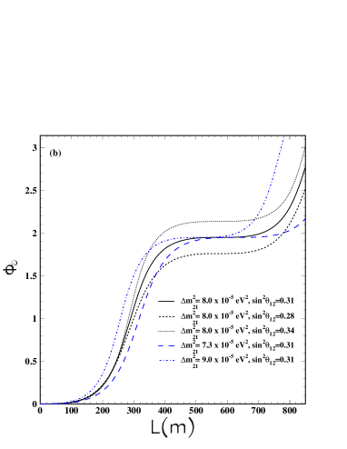
Figure 2: (a) $\phi_{\odot}$ as function of $\Delta_{21}$. $\phi_{\odot}=\pi/2$ when $\Delta_{21}\approx 1.9$.(b) $\phi_{\odot}$ as function of $L$ for various choices of the solar parameters within the current allowed region. $\phi_{\odot}\approx\pi/2$ at about 350 m somewhat independent of the precise values for the solar parameters.

Due to the monotonically increasing nature of $\phi_{\odot}$ and the $\pm$ sign in front of $\phi_{\odot}$, in Eq. (5), for the normal hierarchy the high frequency wiggles undergo a phase advancement as the wave evolves, whereas for the inverted hierarchy there is a phase retardation. It is easy to show that

$$\phi_{\odot}(\Delta_{21}+\pi)=\phi_{\odot}(\Delta_{21})+2\pi\sin^{2}\theta_{12},$$ (8)

i.e. the phase advancement (normal) or retardation (inverted) is $2\pi\sin^{2}\theta_{12}$ for every $\pi$ increase of $\Delta_{21}$. Eqs. (5) and (6) are the foundations of our investigation.

Some important observations are worth emphasizing immediately:

• Only $\Delta_{\text{ee}}$ varies at the atmospheric scale. Everything else, including phase $\phi_{\odot}$, varies at the solar scale. This is a useful distinction because these two scales differ by a factor of $\sim 30$.

• The difference between probabilities corresponding to the two hierarchies (3) is given by

  $${\Delta P\over\sqrt{P(\theta_{13}=0)}} = \sin^{2}2\theta_{13}\sin 2\Delta_{\text{ee}}\sin\phi_{\odot}\,,$$ (9)

  to leading order in $\theta_{13}$. $\Delta P$ becomes visible when the phase $\phi_{\odot}$ develops to order unity. From Fig. 2 this occurs at around the first solar oscillation maximum, ($\Delta_{21}=\pi/2$), in agreement with the features exhibited in Fig. 1. From (9) we also see that the normal and the inverted hierarchies are maximally out of phase when $\phi_{\odot}=\pi/2$. This occurs when

  $$\cot\Delta_{21}\cot(\Delta_{21}\cos 2\theta_{12})=-\cos 2\theta_{12}\,.$$ (10)

  The approximate solution to this equation, for $\theta_{12}$ around 30 degrees, is $\Delta_{21}\approx\frac{\pi}{2}+\cos 2\theta_{12}/(\pi\sin^{2}\theta_{12})$. For $\sin^{2}\theta_{12}=0.31$, Eq. (10) is satisfied when $\Delta_{21}\approx 1.9$, i.e., just beyond the first solar oscillation maximum.

• We notice that by doing transformation $\theta_{12}\rightarrow\pi/2-\theta_{12}$ (or $s_{12}\leftrightarrow c_{12}$) in (6) flips the sign of $\phi_{\odot}$. It means that the mass hierarchy is confused by the presence of the particular type of CPT violation, the subtle one discussed in andre . It occurs because we use the antineutrino channel; If we are able to use the neutrino channel, the problem of confusion does not arise because we know that $\theta_{12}<\pi/4$ from the solar neutrino observation.

II.2 Experimental strategy and requirements to the accuracy of measurement

We now describe our experimental strategy for determining the hierarchy. First one needs to make a very precise measurement of $\Delta m^{2}_{\text{ee}}$ at short distances from the source, at around half the atmospheric oscillation length, $L_{0}/2$ where

$$L_{0}\equiv\frac{4\pi E}{\Delta m^{2}_{\text{ee}}}=18.4\,\left[\frac{E}{18.6\text{ keV}}\right]\left[\frac{\Delta m^{2}_{\text{ee}}}{2.5\times 10^{-3}\text{eV}^{2}}\right]^{-1}\text{m}\,.$$ (11)

Then, one must determine the sign in front of $\phi_{\odot}$ where the phase difference between normal and inverted hierarchy is maximal, i.e. $\Delta_{21}\approx 2$ as can be seen in Fig. 2. With $\Delta_{\text{ee}}/\Delta_{21}\simeq 30$, it can be translated into the distance $L\approx[(2\times 30)/\pi]L_{0}\simeq 20\,L_{0}$ away from the source.

How well do we need to know $\Delta m^{2}_{\text{ee}}$? If we do not know the value of $\Delta m^{2}_{\text{ee}}$ with sufficient precision, one can adjust $\Delta m^{2}_{\text{ee}}$, depending upon the normal (NH) and the inverted (IH) hierarchies, so that the relation

$$2\Delta_{\text{ee}}|_{\text{NH}}+\phi_{\odot}=2\Delta_{\text{ee}}|_{\text{IH}}-\phi_{\odot}$$ (12)

holds at some $L/E$. Then, from Eq. (5) the hierarchy is completely confused as we will explicitly see in Sec. III.1. It can be translated into

$$\frac{\Delta m^{2}_{\text{ee}}|_{\text{IH}}-\Delta m^{2}_{\text{ee}}|_{\text{NH}}}{\Delta m^{2}_{\text{ee}}}\left(\frac{\pi L}{L_{0}}\right)=\phi_{\odot}$$ (13)

which leads to the requirement for the accuracy of measurement of $\Delta m^{2}_{\text{ee}}$ as $\delta(\Delta m^{2}_{\text{ee}})/\Delta m^{2}_{\text{ee}}\raise 1.29167pt\hbox{$\;<$\kern-7.5pt\raise-4.73611pt\hbox{$\sim\;$}}2L_{0}/\pi L\simeq 3$%. This is the critical value at which the hierarchy is completely confused, and if we want to do better, e.g., at least a factor of 3 times better than 3%, the first requirement is $\simeq$1% measurement of $\Delta m^{2}_{\text{ee}}$.

At this point the astute reader will be concerned that we are attempting to determine a oscillation phase after 20 or so oscillations. Aren’t the atmospheric oscillations completely washed out long before 20 $L_{0}$? To observe atmospheric oscillations 20 or so oscillations out, assuming coherence, demands that we can determine $L/E$ per event to high precision. Figure 3 shows how the oscillations are reduced as the resolution on $L/E$ is increased and that a precision better than 1% is required to see oscillation at $\sim$ 20 oscillation lengths from the source.

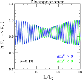
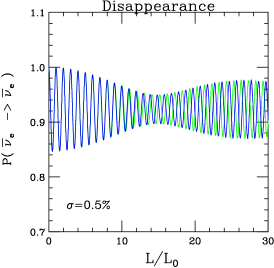
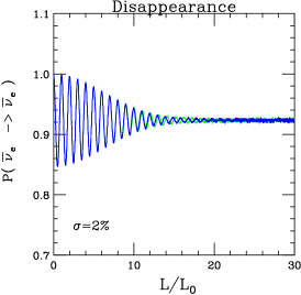
Figure 3: The averaged $P(\nu_{e}\rightarrow\nu_{e})$ versus distance measured in number of oscillation lengths, $L_{0}$. To help with visualization $P_{\odot}=\sin^{2}2\theta_{12}\cos^{4}\theta_{13}\sin^{2}\Delta_{21}$ has been set to zero for these figures. (a) 0.1% Gaussian resolution on $L/E$. (b) 0.5% resolution on $L/E$. (c) 2% resolution on $L/E$. In (b) the oscillations are reduced at 20 or so oscillations out, but still observable. Whereas in (c) the oscillations are averaged out by 15 $L_{0}$.

In summary, to measure the sign of the phase and determine the hierarchy we have two important initial requirements:

• The resolution on $\Delta m^{2}_{\text{ee}}$ measured in a short baseline experiment ($\sim L_{0}/2$ from the source) must be $\simeq$1% or less.

• The resolution on $L/E$ for the long baseline experiment ($\sim$ 20 $L_{0}$ from the source) must be $\simeq$1% or less.

Usually, the neutrino energy cannot be determined experimentally with this accuracy, therefore, these preconditions are very difficult to meet, if not impossible.

II.3 Mass hierarchy reversal and comments on the reactor neutrino method

We have emphasized in the foregoing discussions the importance of identifying the quantity to be held fixed to define the mass hierarchy reversal, and proposed $\Delta m^{2}_{\text{ee}}$ as the solution. In this subsection we want to elaborate this point and clarify how the difference between the normal and the inverted hierarchies can be made artificially larger by choosing different variables to define the hierarchy reversal.

In Fig. 4, presented is the survival probability of electron anti-neutrinos at a baseline of 50 km from a source which is averaged over the uncertainty of energy 3%/$\sqrt{E/\text{MeV}}$ as a function of neutrino energy $E$. It is shown in the left panel of Fig. 4 that if we hold $|\Delta m^{2}_{32}|$ fixed in reversing the hierarchy from the normal to the inverted (as was done in petcov ) the difference between the normal and the inverted hierarchies is clearly visible. However, the obvious distinction seen in the left panel of Fig. 4 disappears if we use $\Delta m^{2}_{\text{ee}}$ to hold when switching between the hierarchies as shown in the middle panel of Fig. 4. A simple explanation for such a marked difference is that by holding $|\Delta m^{2}_{32}|$ fixed in reversing the hierarchy from the normal to the inverted one maps the neutrino mass spectrum into a significantly different one, $|\Delta m^{2}_{31}|_{\text{IH}}=|\Delta m^{2}_{31}|_{\text{NH}}-2\Delta m^{2}_{21}$. (See Appendix A for more about it.) This artificially enhances the difference between the hierarchies, as demonstrated in Fig. 4.

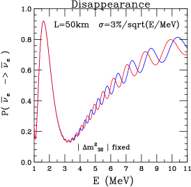
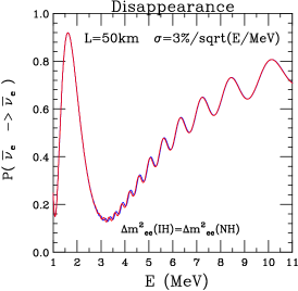
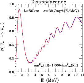
Figure 4: The $\bar{\nu}_{e}$ disappearance probability at 50 km from a reactor source as a function of the neutrino energy. The resolution on the energy is assumed to be 3%/$\sqrt{E/\text{MeV}}$. The blue (light gray) and the red (dark gray) curves are for the normal and the inverted mass hierarchies, respectively. In the left panel $|\Delta m^{2}_{32}|$ is held fixed when the hierarchy is flipped, whereas in the middle panel $\Delta m^{2}_{\text{ee}}$ is held fixed. In the right panel $\Delta m^{2}_{\text{ee}}$ for the inverted hierarchy is 0.6% larger then for the normal hierarchy.

Despite that there exist some discrepancies at energies around 4 MeV, a peak energy of signal events in reactor experiments, the two disappearance probabilities can be made very close to each other over the energy range of 4 to 6 MeV if we allow the value of $\Delta m^{2}_{\text{ee}}$ for the inverted hierarchy to increase by 0.6% relative to the value for the normal hierarchy, as can be seen in the right panel of Fig. 4. The lesson we have learned from this exercise is that unless we know $\Delta m^{2}_{\text{ee}}$ to a sub-percent level, the hierarchy can be easily confused by a tiny shift of the atmospheric $\Delta m^{2}$.

One might want to use neutrinos from reactors to determine the mass hierarchy by the present method, as suggested by the authors of petcov . However, the experimental requirements are very severe in order for this method to work. We believe that the three points discussed above deserve attention if one want to make a reliable estimate of sensitivity to the mass hierarchy resolution with reactor neutrinos; (1) definition of hierarchy reversal, (2) implementation of realistic energy resolution, and (3) robustness of the sensitivity to mass hierarchy resolution against the uncertainty of $\Delta m^{2}_{ee}$.

The recent Hanohano proposal, hanohano , sidesteps some of these requirements by using a sophisticated Fourier transform technique. Detailed analysis around the atmospheric peak in Fourier space can tells us whether $|\Delta m^{2}_{32}|$ is greater or smaller than$|\Delta m^{2}_{31}|$, thus determining the hierarchy. There is no need to explicitly deal with the definition of hierarchy reversal. In this way, the two curves shown in the two right panels of Fig. 4 can, in principle, be distinguished. If this can be achieved in a realistic setting of the experiment, it represents a remarkable advance for reactor neutrino experiments, demonstrating the power of the Fourier transform technique.

III Experimental setup, analysis method and results

Most probably, the unique possibility to satisfy both requirements of the previous section is to make use of monochromatic beam from the bound-state beta decay ${}^{3}\mbox{H}\rightarrow\,^{3}\mbox{He}+\mbox{orbital e}^{-}+\bar{\nu}_{e}$ and detect it by the time-reversed resonant absorption reaction $\bar{\nu}_{e}+^{3}\mbox{He}+\mbox{orbital e}^{-}\rightarrow\,^{3}\mbox{H}$, the idea recently revived by Raghavan Raghavan . For the Mössbauer enhancement to work the method requires $\Delta E/E$ better than $10^{-16}$, a truly monochromatic neutrino beam of 18.6 keV. Thus, the energy spread of the beam in such an experiment is automatically much narrower than what is required.

Having monochromaticity satisfied, the remaining requirement is on the baseline $L$. The short and long baseline measurement are to be done at the distances of $\sim$10 m and $20L_{0}\sim 350$ m from the source, respectively. Then, the requirement on $\Delta L/L$ of, say, 0.3% implies that the size of the source and the target must be limited respectively to $\sim$3 cm and $\sim$1 m in short and long baseline measurement. The former places severe limits on the sizes of the source and the detector. Assuming this requirement can be met, it has been shown by analyzes with several concrete settings that a sensitivity to $\Delta m^{2}_{\text{ee}}$ of $\simeq 0.3~{}(\sin^{2}2\theta_{13}/0.1)^{-1}$% at 1$\sigma$ CL is possible mina-uchi . Therefore, the first requirement listed in Sec. II.2 can be met if $\sin^{2}2\theta_{13}\raise 1.29167pt\hbox{$\;>$\kern-7.5pt\raise-4.73611pt\hbox{$\sim\;$}}$ 0.05.

III.1 Experimental setup and how two-stage measurement works

We consider a possible experimental set up for determination of the neutrino mass hierarchy based on a Mössbauer enhanced $\bar{\nu}_{e}$ absorption experiment Raghavan . By using the revised estimate of the cross section $\sigma_{\text{res}}=0.3\times 10^{-32}\text{cm}^{2}$ Raghavan the event rate is given by

$$R_{\text{enhanced}}=3\times 10^{5}\left(\frac{S\cdot M_{T}}{1\text{MCi}\cdot\text{100 g}}\right)\left(\frac{L}{10~{}\text{m}}\right)^{-2}\text{day}^{-1}.$$ (14)

Therefore, one obtains about one million (2500) events per 3 days (10 days) for 1 MCi source and 100 g ³He target at a baseline distance $L=10$ (350) m. The experiment should be done in two stages; In the first stage, $\Delta m^{2}_{\text{ee}}$ and $\sin^{2}2\theta_{13}$ should be determined very precisely by a measurement at baseline around $\sim$10 m as demonstrated in mina-uchi . We thus do not discuss it further by just assuming the setting with 10 location measurement called the run IIB in mina-uchi . For the second stage, we examine the setting with detectors placed at five locations $L=350\pm(0,5,10)$ m from the source, which covers a complete atmospheric oscillation length. The results of these two stages should be combined as we will discuss bellow.

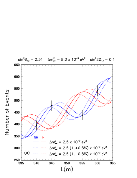
Figure 5: Plotted are the expected number of events to be collected by detectors placed at the distances 340, 345, 350, 355 and 360 m from the source for $\Delta m^{2}_{\text{ee}}=2.5\times 10^{-3}$ eV² and $\sin^{2}2\theta_{13}=0.1$ for the normal hierarchy, indicated by solid circles with error bars. Here $P_{\odot}$ is included (solar parameters are fixed to their best fit values). Expected number of events in the absence of oscillation is assumed to be 2000 at each detector position. The blue (light gray) solid curve which passes through the data points indicates a theoretical expectation assuming the normal hierarchy with $\Delta m^{2}_{\text{ee}}=2.5\times 10^{-3}$ eV² and $\sin^{2}2\theta_{13}=0.1$ whereas the red (dark gray) curve off the data points is the one of inverted hierarchy with same values of $\Delta m^{2}_{\text{ee}}$ and $\theta_{13}$. Assuming that $\Delta m^{2}_{\text{ee}}$ is known to $\pm 0.5$% precision, the thick-dotted (thin-dotted) lines above and below the solid lines are the expectations with $\Delta m^{2}_{\text{ee}}$ 0.5% above (below) that value.

In Fig. 5 we present the expected number of events for $\Delta m^{2}_{\text{ee}}=2.5\times 10^{-3}$ eV² and $\sin^{2}2\theta_{13}=0.1$ at 5 locations mentioned above for the normal hierarchy, for 2000 events at each detector location in the absence of oscillation, which correspond to an exposure of about 20 MCi$\cdot$g$\cdot$day. Throughout our analysis except for that in Sec. IV, we fix the solar parameters to their best fit values as $\sin^{2}\theta_{12}=0.31$ and $\Delta m^{2}_{21}=8.0\times 10^{-5}$ eV² and do not try to vary them. $\Delta m^{2}_{\text{ee}}$ is taken with a tentative expectations for its accuracy, $\Delta m^{2}_{\text{ee}}=2.5\times 10^{-3}(1\pm 0.5$ %) eV². The case of the normal and the inverted hierarchy are plotted by the blue (light gray) and the red (dark gray) curves, respectively. It appears that, if enough statistics is accumulated and $\Delta m^{2}_{\text{ee}}$ is separately measured accurately, the five point measurement, can discriminate between the normal and the inverted hierarchies. The details of the statistical procedure is described in the next subsection.

We show in three panels in Fig. 6 the allowed regions in the $\sin^{2}2\theta_{13}-\Delta m^{2}_{\text{ee}}$ space obtained by the first stage alone (upper panels), by the second stage alone (middle panels), and the one obtained when the first and the second stages are combined (lower panels). The input parameters are taken as $\sin^{2}2\theta_{13}=0.1$, $\Delta m^{2}_{\text{ee}}=2.5\times 10^{-3}$ eV², and the mass hierarchy is assumed to be the normal one. In the first-stage measurement to be done at around the distance $L_{0}/2\simeq 10$ m from the source, $\sin^{2}2\theta_{13}$ as well as $\Delta m^{2}_{\text{ee}}$ can be determined rather precisely. But, there is no sensitivity to the mass hierarchy because the baseline is too short, as is the case of reactor $\theta_{13}$ experiment.

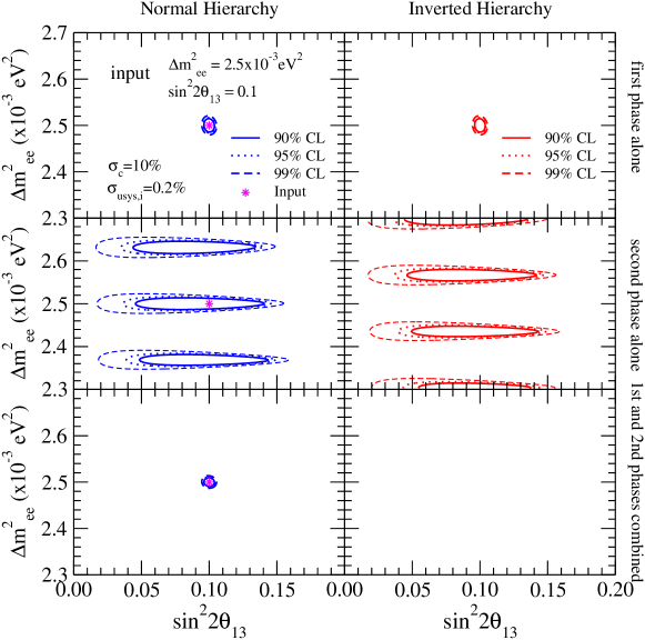
Figure 6: The allowed regions in the $\sin^{2}2\theta_{13}-\Delta m^{2}_{\text{ee}}$ plane obtained by the first stage alone (upper panels), the second stage alone (middle panels) and the combined result of these two stages (lower panels) for the case where the input parameters are $\sin^{2}2\theta_{13}=0.1$, $\Delta m^{2}_{\text{ee}}=2.5\times 10^{-3}$ eV² with the normal hierarchy, based on the $\chi^{2}$ analysis described in Sec. III.2. The solar parameters are fixed to their current best fit values. The first stage is assumed to be performed at 10 positions at around $L\sim 9$ m following the run IIB in mina-uchi whereas the second stage is assumed to be performed at 5 locations at $L=350\pm(0,5,10)$ m from the source. The three closed curves (red, blue, green) from inner to outer denote the ones obtained at 90% CL, 95% CL, and 99 % CL.

The feature of the second-stage experiment presented in the middle panels of Fig. 6 requires some explanations. First of all, there exist many isolated island-like allowed regions. Suppose that $\theta_{13}$ is given from some other experiments. Then, due to the cosine term in Eq. (5) the measurement will give a periodic solution

$$\Delta m^{\prime 2}_{\text{ee}}\approx\Delta m^{2}_{\text{ee}}+\frac{4n\pi E}{L},\ \ (n=\pm 1,\pm 2,...)$$ (15)

for both of the hierarchies. If we take approximation $\phi_{\odot}=\pi/2$, there is a shift $2\pi E/L$ between the adjacent $\Delta m^{2}_{\text{ee}}$ solutions for the normal and the inverted hierarchies. Hence, the solutions of $\Delta m^{2}_{\text{ee}}$ are alternating in the normal and the inverted hierarchies with a constant shift $2\pi E/L$ between the adjacent solutions, the feature clearly visible in the middle panels of Fig. 6. The contours have finite widths, though prolonged, along the $\sin^{2}2\theta_{13}$ direction because the second stage measurement alone can determine $\theta_{13}$ but only with a limited accuracy.

It’s clear that the second stage alone can not determine neither the value of $\Delta m^{2}_{\text{ee}}$ nor the mass hierarchy. However, once the results of the first and the second stages are combined all the fake solutions are eliminated, as demonstrated in the lower panels of Fig. 6. It is evident that $\Delta m^{2}_{\text{ee}}$ must be determined with high accuracy in the first stage measurement.

III.2 Analysis method and definition of $\chi^{2}$

Now we give details of our analysis method. To calculate the sensitivity of the determination of the neutrino mass hierarchy by the first and second stages of the experiment combined, we compute

$$\Delta\chi^{2}_{\text{min}}(\sin^{2}2\theta_{13})=\chi^{2}_{\text{min}}(\rm wrong\;hierarchy)-\chi^{2}_{\text{m}in}(\rm true\;hierarchy)\,,$$ (16)

where $\chi^{2}_{\text{min}}(\rm true/wrong\;hierarchy)$ is the minimum of

$$\chi^{2}(\rm true/wrong\;hierarchy)=\chi^{2}_{1}+\chi^{2}_{2}(\rm true/wrong\;hierarchy)\,,$$ (17)

with the first stage $\chi^{2}$ given by

$$\chi^{2}_{\text{1st}}(\Delta m^{2}_{\text{ee}},\,\sin^{2}2\theta_{13})=\sum_{i,j=1}^{10}\left[\frac{N_{i}^{\text{1-obs}}-N_{i}^{\text{1-theo}}}{N_{i}^{\text{1-theo}}}\right]\,(V^{-1}_{\text{1}})_{ij}\,\left[\frac{N_{j}^{\text{1-obs}}-N_{j}^{\text{1-theo}}}{N_{j}^{\text{1-theo}}}\right]\,,$$ (18)

and the second stage $\chi^{2}$ given by

$$\chi^{2}_{\text{2nd}}(\Delta m^{2}_{\text{ee}},\,\sin^{2}2\theta_{13},\text{sign}(\Delta m^{2}_{31}))=\sum_{i,j=1}^{5}\left[\frac{N_{i}^{\text{2-obs}}-N_{i}^{\text{2-theo}}}{N_{i}^{\text{2-theo}}}\right]\,(V^{-1}_{\text{2-obs}})_{ij}\,\left[\frac{(N_{j}^{\text{2}}-N_{j}^{\text{2-theo}})}{N_{j}^{\text{2-theo}}}\right].$$ (19)

$N_{i}^{\text{1,2-obs}}$ is the number of events at baseline $L_{i}$ for a given input hierarchy and values of the mixing parameters (observed events), while $N_{i}^{\text{1,2-theo}}$ is the theoretically expected number of events at baseline $L_{i}$ for a given set of oscillation parameters. We use, as in Ref. mina-uchi , the correlation matrices

$$(V^{-1}_{\text{1,2}})_{ij}=\frac{\delta_{ij}}{\sigma^{2}_{ui}}-\frac{1}{\sigma^{2}_{ui}\sigma^{2}_{uj}}\frac{\sigma^{2}_{c}}{[1+(\sum_{k}\frac{1}{\sigma^{2}_{uk}})\sigma^{2}_{c}]},$$ (20)

where $\sigma^{2}_{ui}=\sigma^{2}_{\text{usys}}+1/N_{i}^{\text{1,2-th}}$.

The estimation of the uncorrelated systematic uncertainty is the key issue in our sensitivity analysis. In mina-uchi two cases of the error, $\sigma_{\text{usys}}=0.2$ % and 1%, are examined. The former corresponds to the case of movable detector, assuming that a direct extraction or real-time detection of produced ³H atom is possible. The latter is a tentative estimate for the case of multiple identical detectors. We use the correlated systematic uncertainty $\sigma_{c}=10$ %, though the results are insensitive to $\sigma_{c}$. We adopt the same numbers as these for the uncertainties in our analysis for both the first and the second stages of the experiment.

In our $\chi^{2}$ analysis, for simplicity, the solar mixing parameters are fixed to the current best fit values, ignoring their uncertainties. Therefore, the fitting parameters are: $\Delta m^{2}_{\text{ee}}$, $\sin^{2}2\theta_{13}$ and the sign of $\Delta m^{2}_{31}$. Note, however, that $\chi^{2}_{\text{1st}}$ for the first stage has practically no dependence on solar parameters as well as the mass hierarchy due to too short baseline. The current uncertainty on the values of the solar parameter are not so relevant for the determination for the hierarchy because $\phi_{\odot}$ does not depend strongly on them (see Fig. 2b) as pointed out previously.

III.3 Sensitivity to mass hierarchy determination

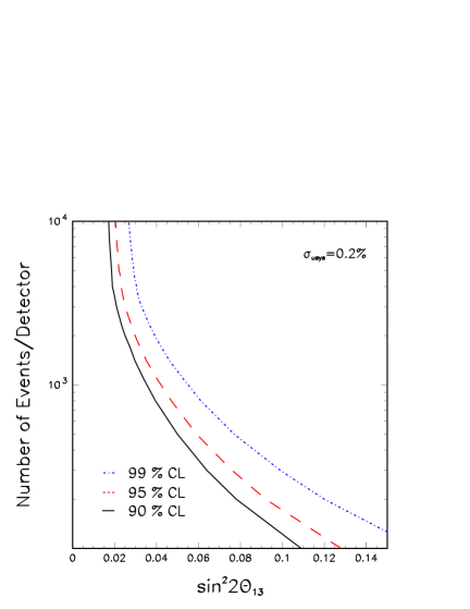
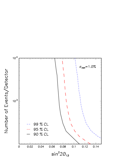
Figure 7: The region of sensitivity to resolving the mass hierarchy in $\sin^{2}2\theta_{13}-$event number (per detector) space. The black solid, the red dashed, and the blue dotted curves denote the region boundary at 90%, 95%, and 99% CL, respectively. The left and right panels are for the cases of uncorrelated systematic uncertainties of 0.2% and 1%, respectively.

Now, we present our estimation of the sensitivity of the two-stage Mössbauer $\bar{\nu}_{e}$ experiment to the determination of the neutrino mass hierarchy. In Fig. 7 we present the region of sensitivity to resolving the mass hierarchy at 90%, 95%, and 99% CL, denoted by the black solid, the red dashed, and the blue dotted curves, respectively. The abscissa is $\sin^{2}2\theta_{13}$ and the ordinate is the number of events per detector in long baseline experiment. Here, 90%, 95%, and 99% CL correspond to $\Delta\chi^{2}_{\text{min}}=\chi^{2}_{\text{min}}(\rm wrong\;hierarchy)-\chi^{2}_{\text{m}in}(\rm true\;hierarchy)$ = 2.71, 3.84 and 6.63, respectively. Left and right panels are for the cases where the uncorrelated systematic uncertainty is 0.2% and 1%, respectively.

Assuming $\sigma_{\text{usys}}=0.2$ %, we can see that the hierarchy can be determined at 90 (99) % CL for $\sin^{2}2\theta_{13}$ down to 0.035 (0.06) for 1000 events and down to 0.025 (0.04) for 2000 events. For a larger error $\sigma_{\text{usys}}=1$%, the critical value of $\sin^{2}2\theta_{13}$ will be $\sim$ 0.08 (0.11) at 90 (99) % CL approximately independent of the number of events larger than $\sim$ 1000. This is caused by the fact that the precision on the determination of $\Delta m^{2}_{\text{ee}}$ at the first stage is highly dependent on this systematic uncertainty mina-uchi .

IV Determination of the Solar Parameters

In the second stage of the Mössbauer experiment, the detectors are placed just after the first solar oscillation maximum in order to determine the mass hierarchy, as we discussed in the previous section. In a possible third stage of the experiment, one could envisage moving the detectors somewhat closer to the source in order to cover the region around this maximum. It will allow us a precise determination of the solar-scale oscillation parameters, $\Delta m^{2}_{21}$ and $\theta_{12}$.

In order to optimize the determination of these parameters, we assume that the measurements will be performed at the following 10 different detector locations,

$$L_{n} = [200+50\,(n-1)]\;{\rm m},$$ (21a)

$$L^{\prime}_{n} = L_{n}-L_{0}/2,\quad\quad n=1,2,..,5.$$ (21b)

First, in order to observe the oscillation driven by the solar $\Delta m_{21}^{2}$, we consider the configuration of 5 detector locations ($L_{n}$) separated by 50 m, ranging from 200 m to 400 m as in Eq. (21a). In this way, we can cover the whole range of solar-scale oscillation before and after the dip due to the oscillation maximum (see Fig. 1). Second, in order to minimize the unwanted effect due to the rapid oscillations driven by the atmospheric $\Delta m_{\text{ee}}^{2}$, we have to place, for each location $L_{n}$, another detector (or move detector to another location) at $L^{\prime}_{n}$ separated from $L_{n}$ by half the atmospheric oscillation length, $L_{0}/2$. See Eq. (21b). The setting of five pairs of detector locations works because the average of the oscillation probabilities corresponding to these two positions $L_{n}$ and $L^{\prime}_{n}$ is, at first approximation, independent of $\theta_{13}$ and $\Delta m_{\text{ee}}^{2}$ and thus is free from any ambiguity associated with the atmospheric oscillations.

In this calculation we assume that the exposure is such that the same number of events (1000) in the absence of oscillation are collected at each detector location. We take the pessimistic value of the systematic uncertainty $\sigma_{\rm usys}=$ 1% instead of 0.2 % because the results do not differ much; The sensitivity is still dominated by the statistics in this regime. As in the previous sections, the input values of the other oscillation parameters are fixed as $\Delta m^{2}_{\text{ee}}=2.5\times 10^{-3}$ eV², $\sin^{2}\theta_{12}=0.31$ and $\Delta m^{2}_{21}=8.0\times 10^{-5}$ eV².

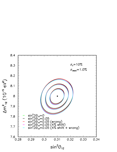
Figure 8: Expected allowed regions in the plane $\sin^{2}\theta_{12}-\Delta m^{2}_{21}$ for 1000 events taken at each detector position at 68.27% (inner curves), 95.0% (middle curves) and 99.73% (outer curves) CL for 2 DOF. We assumed the measurement will be done at 10 different detector locations, $L_{n}=[200+50\;(n-1)]$ m and $L^{\prime}_{n}=L_{n}-L_{0}/2$ with $n=1,2,...,5$. The input values used are: $\sin^{2}\theta_{12}=0.31$, $\Delta m^{2}_{21}=8.0\times 10^{-5}$ eV², $\Delta m^{2}_{\text{ee}}=2.5\times 10^{-3}$ eV². The green and black curves are for the input values of $\sin^{2}2\theta_{13}=0$ and $0.05$, respectively. The other curves are also for $\sin^{2}2\theta_{13}=0.05$ but fitted with: the wrong hierarchy (red), $\Delta m^{2}_{\text{ee}}$ shifted by 4% (magenta) and the wrong hierarchy and $\Delta m^{2}_{\text{ee}}$ shifted by 4% (cyan). Here we have supposed $\sigma_{\text{usys}}=$ 1%.

In Fig. 8 we show how well $\Delta m^{2}_{21}$ and $\sin^{2}\theta_{12}$ can be determined by this experiment. The obtained sensitivity contours with $\sin^{2}\theta_{13}=0$ are presented by the green lines (which practically overlapped with the black ones) in Fig. 8. From this result, we conclude that the precision one can achieve for $\sin^{2}\theta_{12}$ is about 1.6 (4.0) % at 68.27 (99.73) % CL for 2 DOF whereas that for $\Delta m^{2}_{21}$ is about 0.9 (2.2) % at 68.27 (99.73) % CL for 2 DOF. Comparing this result with the sensitivity which can be achieved by the dedicated reactor experiment for the similar number of events studied in Ref. sado+others , the precision we obtained for $\sin^{2}\theta_{12}$ and $\Delta m^{2}_{21}$ in this work are comparable or better, in particular, for $\Delta m^{2}_{21}$ (see e.g. Fig. 5 of the first article in  sado+others ).

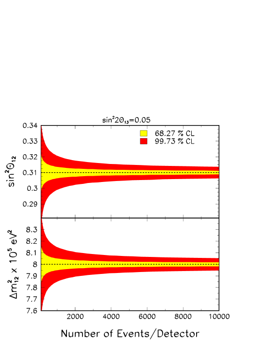
Figure 9: Determination of $\sin^{2}\theta_{12}$ (upper panel) and $\Delta m^{2}_{21}$ (lower panel) as a function of detector exposure at 68.27% and 99.73% CL for 1 DOF. Here $\sigma_{\rm usys}=1\%$. The dashed lines show the input values.

In the above argument, we have assumed that $L_{0}$ (or $\Delta m_{\text{ee}}^{2}$) can be determined very precisely in the first stage of the experiment allowing us to place the detector pair separated exactly by $L_{0}/2$. In reality, however, the determination of $L_{0}$ will always carry some uncertainties. Moreover, if $\sin^{2}2\theta_{13}$ is too small or the uncorrelated systematic uncertainty ($\sigma_{\text{usys}}$) is not small enough, the neutrino mass hierarchy will not be determined in the second stage. Then, the question is; What is the additional ambiguities that occur in determination of the solar oscillation parameters in the presence of these uncertainties? Fortunately, we can show that our choice of detector locations defined in Eqs. (21a) and (21b) guarantees that these uncertainties will not deteriorate the precision in the determination of the solar parameters.

In order to check the stability of the results against the uncertainties mentioned above, we performed a fit by assuming the incorrect mass hierarchy and/or slightly incorrect value of $\Delta m^{2}_{\text{ee}}$ by shifting its value by 4%. The results are shown by the blue, the magenta and the light blue curves in Fig. 8 where we can see that for each CL, all the curves are very close to each other, indicating that our results are quite stable against these uncertainties.

We also examine the stability of the sensitivities to possible nonzero values of $\theta_{13}$. In Fig. 8 we show the sensitivity contours for the input values of $\sin^{2}2\theta_{13}=0.05$ (black curve) in comparison to that with $\sin^{2}2\theta_{13}=0.0$ (green curve). We note that these 2 curves are very close to each other implying that the effect of nonzero $\theta_{13}$ is quite small. We emphasize that this feature is in a marked contrast with any of the alternative methods for measuring $\theta_{12}$, including the reactor sado+others and the solar neutrino methods nakahata . In these methods there is no way, unless determined by some other experiments, to control the errors which comes from nonzero $\theta_{13}$ concha-pena , whereas in our present method, there is a built-in mechanism which eliminates the uncertainties that come from the atmospheric oscillation parameters, in particular from $\theta_{13}$.

In Fig. 9 we show how the precision for 1 DOF of each of the solar parameters improves with statistics, that is, as a function of the number of events that would be collected at each detector in the absence of oscillation. As in the previous plot, we have assumed that $\sigma_{\rm usys}=$ 1%. We observe that until $\sim 1000$ events, the precision improves rapidly as the number of events increase and then after, the rapidness of the improvement become smaller. The ultimate precision which can be achieved in the limit of very large statistics with $\sim 10000$ events (per detector) for $\sigma_{\rm usys}=$ 1% would be $\sim$ 0.4 (1.2) % for 68.27% (99.73%) CL for $\sin^{2}\theta_{12}$ and $\sim$ 0.2 (0.7) % for 68.27% (99.73%) CL for $\Delta m^{2}_{21}$. Notice that measurement of $\Delta m^{2}$ to the accuracy of sub % level is usually not possible because the absolute energy scale of leptons is hard to be determined at such accuracy, and it acts as a limiting factor for reducing the $\Delta m^{2}$ error MNPZ . In our case, monochromaticity of the $\bar{\nu}_{e}$ beam with known energy removes the necessity for such calibration for determining absolute energy scale.

V Concluding Remarks

In this paper, we have shown that the neutrino mass hierarchy can be determined only by a single experiment based on resonant $\bar{\nu}_{e}$ absorption reaction enhanced by the Mössbauer effect. In its first stage, $\Delta m^{2}_{\text{ee}}$ must be accurately determined by $L\sim$10 m measurements. In the second stage of the experiment, the relative phase of the atmospheric oscillation (wiggles) between the normal vs. inverted mass hierarchies, phase advancement or retardation must be discriminated by measurements at $L\sim$350 m. It can be executed thanks to the ultra monochromatic nature of neutrino beam which would allow us to detect relative phase of atmospheric oscillation even after 20 oscillations. We stress that the monochromaticity is special to the resonant $\bar{\nu}_{e}$ absorption reaction, most probably the unique experimental way to realize this principle.

We concluded that assuming $\sigma_{\text{usys}}=0.2$ %, the hierarchy can be determined at 90 (99) % CL for $\sin^{2}2\theta_{13}$ down to 0.035 (0.06) for 1000 events collected at five different positions and down to 0.025 (0.04) for 2000 events. For a larger error $\sigma_{\text{usys}}=1$%, the critical value of $\sin^{2}2\theta_{13}$ will be $\sim$ 0.08 (0.11) at 90 (99) % CL approximately independent of the number of events for more than $\sim$ 1000 events.

We have also shown that in a third stage of the experiment, by positioning detectors in different locations, it is possible to determine the solar-scale parameters too. The precision one can achieve with 1000 events in each detector for $\sin^{2}\theta_{21}$ is about 1.6 (4.0) % at 68.27 (99.73) % CL whereas that for $\Delta m^{2}_{21}$ is about 0.9 (2.2) % at 68.27 (99.73) % CL, all for 2 DOF. The accuracies improve as data taking proceeds and the errors would reduce by a factor of $\simeq 3$ when an order of magnitude larger number of events is taken.

It is in fact remarkable that the experimental set up considered in this paper allows us to make a precise measurement of all the mixing parameters appear in the oscillation probability for $\nu_{e}\to\nu_{e}$ channel, $\theta_{12}$, $\theta_{13}$, $\Delta m^{2}_{21}$, $\Delta m^{2}_{\text{ee}}$ and the neutrino mass hierarchy only by a single experiment, independent of any other experiments. The only parameters inaccessible by the method are $\theta_{23}$ and the CP phase $\delta$, but precision measurement of the other mixing parameters will certainly help in determining these parameters by other experiments.

Some remarks are in order:

• As noted in Sec. II.1, our method of determining the mass hierarchy can be confused by the CPT violation of the type with $\theta_{12}$ in different octants in the neutrino and the antineutrino sectors. It in turn implies that once the mass hierarchy is determined by some other means, the measurement we propose in this paper can be regarded as testing that particular type of CPT violation.

• Due to the capability of resolving atmospheric wiggles even after 20 atmospheric oscillations away from the source, this experiment could be sensitive to other dynamics various which differ from the standard three flavor mass induced oscillation one. In particular, one can perhaps probe mechanisms such as: neutrino decay decay , decoherence decoh , mixing with sterile neutrinos sterile , violation of Lorentz invariance or the equivalence principle VEPVLI , long-range leptonic forces LR , extra-dimensions extradim .

Finally, we emphasize that realizing the proposed Mössbauer $\bar{\nu}_{e}$ experiment is crucial in order to make all the discussions in this paper meaningful. The principle of the experiment is well formulated by having the decay producing source $\bar{\nu}_{e}$ and the absorption reaction in the target as T-conjugate channels with each other, allowing mutual cancellation of large part of the atomic shift Raghavan ; raghavan_now2006 . Nonetheless, it still remains unclear to what extent the ³He atom in the target experiences exactly the same environment as the ³H atom in the source potzel_snow2006 . This point has to be (and will be) investigated in a systematic way. If the experiment is indeed realizable it will certainly open a new window for neutrino experiments which can explore the neutrino properties in otherwise inaccessible manner.

Appendix A The Effective Atmospheric $\Delta m^{2}$

The advancement or retardation of the phase, $\phi_{\odot}$, could be interpreted as a change in the effective atmospheric $\Delta m^{2}$. Such an effective atmospheric $\Delta m^{2}$, at $L/E$, is naturally defined by

$$\Delta m^{2}_{\text{eff}}(L/E) \equiv \frac{d~{}(2\Delta_{\text{ee}}\pm\phi_{\odot})}{d~{}(L/2E)}=\Delta m^{2}_{\text{ee}}\pm\frac{1}{2}~{}\Delta m^{2}_{21}\cos 2\theta_{12}~{}\frac{\sin^{2}2\theta_{12}\sin^{2}\Delta_{21}}{1-\sin^{2}2\theta_{12}\sin^{2}\Delta_{21}}$$

$$= \left(\frac{c^{2}_{12}-\frac{1}{2}\sin^{2}2\theta_{12}\sin^{2}\Delta_{21}}{1-\sin^{2}2\theta_{12}\sin^{2}\Delta_{21}}\right)|\Delta m^{2}_{31}|+\left(\frac{s^{2}_{12}-\frac{1}{2}\sin^{2}2\theta_{12}\sin^{2}\Delta_{21}}{1-\sin^{2}2\theta_{12}\sin^{2}\Delta_{21}}\right)|\Delta m^{2}_{32}|.$$

Where the positive (negative) sign, in Eq. (A), is for the normal (inverted) hierarchy. For $\Delta_{21}\ll 1$ we recover $\Delta m^{2}_{\text{ee}}$, since this is in essence its definition, see Ref. NPZ for details. Thus Eq. (A) is the generalization of $\Delta m^{2}_{\text{ee}}$ to arbitrary $L/E$. In Fig. 10 we show the variation of $\Delta m^{2}_{\text{eff}}$ as a function of baseline for both the normal and inverted hierarchies. The extrema of the difference between $\Delta m^{2}_{\text{eff}}(L/E)$ and $\Delta m^{2}_{\text{ee}}$ are given by

$$\frac{1}{2}~{}\Delta m^{2}_{21}\cos 2\theta_{12}~{}\frac{\sin^{2}2\theta_{12}\sin^{2}\Delta_{21}}{1-\sin^{2}2\theta_{12}\sin^{2}\Delta_{21}} = \left\{\begin{array}[]{ll}0&{\rm at}~{}\Delta_{21}=n\pi\\ \frac{1}{2}~{}\frac{\sin^{2}2\theta_{12}}{\cos 2\theta_{12}}~{}\Delta m^{2}_{21}&{\rm at}~{}\Delta_{21}=(2n-1)\pi/2.\end{array}\right.$$ (25)

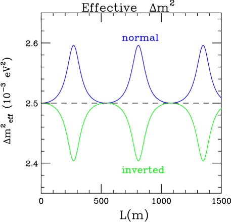
Figure 10: $\Delta m^{2}_{\text{eff}}$ as function of baseline at 18.6 keV neutrino energy for both the normal and inverted hierarchies. The dashed line is $\Delta m^{2}_{\text{ee}}$ which has been assumed to be the same for the normal and inverted hierarchies for this plot. In general, unless $\Delta m^{2}_{\text{ee}}$ is determined precisely it need not take exactly the same value for both hierarchies. The maximum difference between $\Delta m^{2}_{\text{eff}}$ and $\Delta m^{2}_{\text{ee}}$ occurs at the solar oscillation maxima, i.e. when $\Delta_{21}=(2n-1)\pi/2$.

As the oscillations go through the solar maxima, the fractional increase (decrease) in the effective atmospheric $\Delta m^{2}$ is

$$\frac{1}{2}~{}\frac{\sin^{2}2\theta_{12}}{\cos 2\theta_{12}}~{}\frac{\Delta m^{2}_{21}}{\Delta m^{2}_{\text{ee}}}\approx 4\%\,,$$ (26)

for the normal (inverted) hierarchy. It is the accumulated effect of this small difference in the effective atmospheric $\Delta m^{2}$ for the normal and inverted hierarchies that leads to the observable phase difference shown in Fig. 1. Since

$$\frac{1}{2}\int_{0}^{L/E}d(L/E)~{}\Delta m^{2}_{\text{eff}}(L/E)=(2\Delta_{\text{ee}}\pm\phi_{\odot})|_{L/E},$$ (27)

as it must.

Appendix B $\nu_{\mu}$ Disappearance

For $\nu_{\mu}$ disappearance in vacuum, most of the results of this paper can be applied, using the following translation

$$\sin^{2}\theta_{12}\Rightarrow\frac{|U_{\mu 2}|^{2}}{|U_{\mu 1}|^{2}+|U_{\mu 2}|^{2}}\quad {\rm and} \quad\sin^{2}\theta_{13}\Rightarrow|U_{\mu 3}|^{2}.$$ (28)

With this translation the atmospheric $\Delta m^{2}_{\mu\mu}$ and phase, $\phi^{\mu}_{\odot}$, are given by

$$\Delta m^{2}_{\mu\mu} \equiv \frac{|U_{\mu 1}|^{2}|\Delta m^{2}_{31}|+|U_{\mu 2}|^{2}|\Delta m^{2}_{32}|}{|U_{\mu 1}|^{2}+|U_{\mu 1}|^{2}}$$ (29)

$${\rm and}\quad\phi^{\mu}_{\odot} = \arctan\left(\frac{|U_{\mu 1}|^{2}-|U_{\mu 2}|^{2}}{|U_{\mu 1}|^{2}+|U_{\mu 2}|^{2}}\tan\Delta_{21}\right)-\frac{|U_{\mu 1}|^{2}-|U_{\mu 2}|^{2}}{|U_{\mu 1}|^{2}+|U_{\mu 2}|^{2}}\Delta_{21}.$$ (30)

Then

$$P(\nu_{\mu}\rightarrow\nu_{\mu})=1-4|U_{\mu 2}|^{2}|U_{\mu 1}|^{2}\sin^{2}\Delta_{21}$$

$$-2|U_{\mu 3}|^{2}(1-|U_{\mu 3}|^{2})\left[1-\sqrt{1-\frac{4|U_{\mu 1}|^{2}|U_{\mu 2}|^{2}}{(|U_{\mu 1}|^{2}+|U_{\mu 2}|^{2})^{2}}\sin^{2}\Delta_{21}}~{}\cos(2\Delta_{\mu\mu}\pm\phi^{\mu}_{\odot})\right].$$ (31)

Since numerically

$$\frac{|U_{\mu 1}|^{2}-|U_{\mu 2}|^{2}}{|U_{\mu 1}|^{2}+|U_{\mu 2}|^{2}}\approx-\cos 2\theta_{12}$$ (32)

the phase for $\nu_{\mu}$ disappearance is approximately minus the phase for $\nu_{e}$ disappearance, i.e.

$$\phi^{\mu}_{\odot}\approx-\phi^{e}_{\odot}.$$ (33)

Therefore the normal hierarchy is retarded while the inverted hierarchy is advanced. This is the opposite sign to what happens for $\nu_{e}$ disappearance but the rate of change is approximately the same.

The effective atmospheric $\Delta m^{2}$ for $\nu_{\mu}$ disappearance at any $L/E$ is given by

$$\Delta m^{2}_{\text{eff}}(\mu\mu) = \left[\frac{|U_{\mu 1}|^{2}(|U_{\mu 1}|^{2}+|U_{\mu 2}|^{2})-2|U_{\mu 1}|^{2}|U_{\mu 2}|^{2}\sin^{2}\Delta_{21}}{(|U_{\mu 1}|^{2}+|U_{\mu 2}|^{2})^{2}-4|U_{\mu 1}|^{2}|U_{\mu 2}|^{2}\sin^{2}\Delta_{21}}\right]|\Delta m^{2}_{31}|$$ (34)

$$\quad+\left[\frac{|U_{\mu 2}|^{2}(|U_{\mu 1}|^{2}+|U_{\mu 2}|^{2})-2|U_{\mu 1}|^{2}|U_{\mu 2}|^{2}\sin^{2}\Delta_{21}}{(|U_{\mu 1}|^{2}+|U_{\mu 2}|^{2})^{2}-4|U_{\mu 1}|^{2}|U_{\mu 2}|^{2}\sin^{2}\Delta_{21}}\right]|\Delta m^{2}_{32}|.$$

Again for small $\Delta_{21}$ this reduces to $\Delta m^{2}_{\mu\mu}$ given by Eq. (29).

For $\nu_{\tau}$ disappearance, just replace $|U_{\mu j}|^{2}$ with $|U_{\tau j}|^{2}$ in the equations of this appendix.

References

- (1) For a recent review, see R. N. Mohapatra and A. Y. Smirnov, Ann. Rev. Nucl. Part. Sci. 56, 569 (2006) [arXiv:hep-ph/0603118].
- (2) V. D. Barger, S. Geer, R. Raja and K. Whisnant, Phys. Lett. B 485, 379 (2000) [arXiv:hep-ph/0004208]; A. Cervera, A. Donini, M. B. Gavela, J. J. Gomez Cadenas, P. Hernandez, O. Mena and S. Rigolin, Nucl. Phys. B 579, 17 (2000) [Erratum-ibid. B 593, 731 (2001)] [arXiv:hep-ph/0002108]; H. Minakata and H. Nunokawa, JHEP 0110, 001 (2001) [arXiv:hep-ph/0108085]. P. Huber, M. Lindner and W. Winter, Nucl. Phys. B 645, 3 (2002) [arXiv:hep-ph/0204352]; V. Barger, D. Marfatia and K. Whisnant, Phys. Rev. D 65, 073023 (2002) [arXiv:hep-ph/0112119]; H. Minakata, H. Nunokawa and S. J. Parke, Phys. Rev. D 68, 013010 (2003) [arXiv:hep-ph/0301210]; O. Mena and S. J. Parke, Phys. Rev. D 70, 093011 (2004) [arXiv:hep-ph/0408070]; O. Mena Requejo, S. Palomares-Ruiz and S. Pascoli, Phys. Rev. D 72, 053002 (2005) [arXiv:hep-ph/0504015]. M. Ishitsuka, T. Kajita, H. Minakata and H. Nunokawa, Phys. Rev. D 72, 033003 (2005) [arXiv:hep-ph/0504026].
- (3) D. Beavis et al., arXiv:hep-ex/0205040; M. V. Diwan et al., Phys. Rev. D 68, 012002 (2003) [arXiv:hep-ph/0303081]; V. Barger, M. Dierckxsens, M. Diwan, P. Huber, C. Lewis, D. Marfatia and B. Viren, Phys. Rev. D 74, 073004 (2006) [arXiv:hep-ph/0607177]; R. Gandhi, P. Ghoshal, S. Goswami, P. Mehta and S. Uma Sankar, Phys. Rev. D 73, 053001 (2006) [arXiv:hep-ph/0411252].
- (4) T. Kajita, Talk given at Next Generation of Nucleon Decay and Neutrino Detectors (NNN05), Aussois, Savoie, France, April 7-9, 2005. http://nnn05.in2p3.fr/; S. Palomares-Ruiz and S. T. Petcov, Nucl. Phys. B 712, 392 (2005) [arXiv:hep-ph/0406096]; S. T. Petcov and T. Schwetz, Nucl. Phys. B 740, 1 (2006) [arXiv:hep-ph/0511277]; R. Gandhi, P. Ghoshal, S. Goswami, P. Mehta and S. Uma Sankar, arXiv:hep-ph/0506145.
- (5) A. de Gouvea, J. Jenkins and B. Kayser, Phys. Rev. D 71, 113009 (2005) [arXiv:hep-ph/0503079];
- (6) H. Nunokawa, S. J. Parke and R. Zukanovich Funchal, Phys. Rev. D 72, 013009 (2005) [arXiv:hep-ph/0503283].
- (7) H. Minakata, H. Nunokawa, S. J. Parke and R. Zukanovich Funchal, Phys. Rev. D 74, 053008 (2006) [arXiv:hep-ph/0607284].
- (8) A. S. Dighe and A. Y. Smirnov, Phys. Rev. D 62, 033007 (2000) [arXiv:hep-ph/9907423]; H. Minakata and H. Nunokawa, Phys. Lett. B 504, 301 (2001) [arXiv:hep-ph/0010240]; C. Lunardini and A. Y. Smirnov, JCAP 0306, 009 (2003) [arXiv:hep-ph/0302033]; V. Barger, P. Huber and D. Marfatia, Phys. Lett. B 617, 167 (2005) [arXiv:hep-ph/0501184].
- (9) A. S. Dighe, M. T. Keil and G. G. Raffelt, JCAP 0306, 005 (2003) [arXiv:hep-ph/0303210]; ibid. 0306, 006 (2003) [arXiv:hep-ph/0304150]; R. Tomas, M. Kachelriess, G. Raffelt, A. Dighe, H. T. Janka and L. Scheck, JCAP 0409, 015 (2004) [arXiv:astro-ph/0407132].
- (10) S. Pascoli, S. T. Petcov and T. Schwetz, Nucl. Phys. B 734, 24 (2006) [arXiv:hep-ph/0505226]; S. Choubey and W. Rodejohann, Phys. Rev. D 72, 033016 (2005) [arXiv:hep-ph/0506102].
- (11) S. T. Petcov and M. Piai, Phys. Lett. B 533, 94 (2002) [arXiv:hep-ph/0112074]. S. Choubey, S. T. Petcov and M. Piai, Phys. Rev. D 68, 113006 (2003) [arXiv:hep-ph/0306017].
- (12) J. Learned, S. Dye, S. Pakvasa and R. Svoboda, arXiv:hep-ex/0612022.
- (13) L. A. Mikaelyan, B. G. Tsinoev, and A. A. Borovoi, Sov. J. Nucl. Phys. 6, 254 (1968) [Yad. Fiz. 6, 349 (1967)].
- (14) R. S. Raghavan, arXiv:hep-ph/0601079.
- (15) W. M. Visscher, Phys. Rev. 116, 1581 (1959); W. P. Kells and J. P. Schiffer, Phys. Rev. C 28, 2162 (1983).
- (16) J. N. Bahcall, Phys. Rev. 124, 495 (1961).
- (17) H. Minakata and S. Uchinami, New J. Phys. 8, 143 (2006) [arXiv:hep-ph/0602046].
- (18) A. de Gouvea and W. Winter, Phys. Rev. D 73, 033003 (2006) [arXiv:hep-ph/0509359].
- (19) W. M. Yao et al. [Particle Data Group], J. Phys. G 33,1 (2006).
- (20) A. de Gouvea and C. Pena-Garay, Phys. Rev. D 71, 093002 (2005) [arXiv:hep-ph/0406301].
- (21) H. Minakata, H. Nunokawa, W. J. C. Teves and R. Zukanovich Funchal, Phys. Rev. D 71, 013005 (2005) [arXiv:hep-ph/0407326]; Nucl. Phys. Proc. Suppl. 145, 45 (2005) [arXiv:hep-ph/0501250]; A. Bandyopadhyay, S. Choubey, S. Goswami and S. T. Petcov, Phys. Rev. D 72, 033013 (2005) [arXiv:hep-ph/0410283]; J. F. Kopp, M. Lindner, A. Merle and M. Rolinec, arXiv:hep-ph/0606151; S. T. Petcov and T. Schwetz, arXiv:hep-ph/0607155.
- (22) M. Nakahata, Talk at the 5th Workshop on “Neutrino Oscillations and their Origin” (NOON2004), February 11-15, 2004, Odaiba, Tokyo, Japan. http://www-sk.icrr.u-tokyo.ac.jp/noon2004/
- (23) M. C. Gonzalez-Garcia and C. Peña-Garay, Phys. Lett. B 527, 199 (2002) [arXiv:hep-ph/0111432].
- (24) M. C. Gonzalez-Garcia and M. Maltoni, Phys. Rev. D 70, 033010 (2004) [arXiv:hep-ph/0404085]; R. Foot, C. N. Leung and O. Yasuda, Phys. Lett. B 443, 185 (1998) [arXiv:hep-ph/9809458].
- (25) J. F. Beacom and N. F. Bell, Phys. Rev. D 65, 113009 (2002) [arXiv:hep-ph/0204111].
- (26) F. Benatti and R. Floreanini, JHEP 0002, 032 (2000) [arXiv:hep-ph/0002221]; F. Benatti and R. Floreanini, Phys. Rev. D 64, 085015 (2001) [arXiv:hep-ph/0105303]; A. M. Gago, E. M. Santos, W. J. C. Teves and R. Zukanovich Funchal, Phys. Rev. D 63, 073001 (2001) [arXiv:hep-ph/0009222]; ibid, arXiv:hep-ph/0208166.
- (27) M. Cirelli, G. Marandella, A. Strumia and F. Vissani, Nucl. Phys. B 708, 215 (2005) [arXiv:hep-ph/0403158]; A. Y. Smirnov and R. Zukanovich Funchal, Phys. Rev. D 74, 013001 (2006)[arXiv:hep-ph/0603009].
- (28) M. Gasperini, Phys. Rev. D 38 (1988) 2635; M. Gasperini, Phys. Rev. D 39, 3606 (1989); S. L. Glashow, A. Halprin, P. I. Krastev, C. N. Leung and J. T. Pantaleone, Phys. Rev. D 56, 2433 (1997) [arXiv:hep-ph/9703454]; S. R. Coleman and S. L. Glashow, Phys. Rev. D 59, 116008 (1999) [arXiv:hep-ph/9812418]; H. Minakata and H. Nunokawa, Phys. Rev. D 51, 6625 (1995) [arXiv:hep-ph/9405239]; G. L. Fogli, E. Lisi, A. Marrone and G. Scioscia, Phys. Rev. D 60, 053006 (1999) [arXiv:hep-ph/9904248].
- (29) L. Okun, Sov. J. Nucl. Phys. 10, 206 (1969), ibid, Phys. Lett. B 382, 389 (1996); J. A. Grifols and E. Masso, Phys. Lett. B 396, 201 (1997) [arXiv:astro-ph/9610205]; J. A. Grifols and E. Masso, Phys. Lett. B 579, 123 (2004) [arXiv:hep-ph/0311141]; M. C. Gonzalez-Garcia, P. C. de Holanda, E. Masso and R. Zukanovich Funchal, JCAP 0701, 005 (2007) [arXiv:hep-ph/0609094].
- (30) G. R. Dvali and A. Y. Smirnov, Nucl. Phys. B 563, 63 (1999) [arXiv:hep-ph/9904211].
- (31) R. S. Raghavan, talk given at Neutrino Oscillation Workshop (NOW2006), Conca Specchiulla, Otranto, Lecce, Italy, September 9-16, 2006, avilable at http://www.ba.infn.it/now/now2006/
- (32) W. Potzel, Phys. Scripta T127, 85 (2006).