Searching for the Kaluza-Klein Graviton in Bulk RS Models

The best-studied version of the RS1 model has all the Standard Model particles confined to the TeV brane. However, recent variants have the Standard Model fermions and gauge bosons located in the bulk five-dimensional spacetime. We study the potential reach of the LHC in searching for the lightest KK partner of the graviton in the most promising such models in which the right-handed top is localized very near the TeV brane and the light fermions are localized near the Planck brane. We consider both detection and the establishment of the spin-2 nature of the resonance should it be found.

1 Introduction

RS models with Standard Model particles in the bulk are a viable possibility for two reasons. The first is that the solution to the hierarchy problem requires only that the Higgs particle is on the TeV brane. Standard Model particles can be either in the bulk or on the brane. The second important feature of RS1 is that the higher-dimensional space, the fourth spatial dimension, is quite small, only of order 35 times the AdS length. Because of this feature, gauge bosons can be in the bulk without the coupling being too strong, since the forces are not very highly diluted. Such models, with the Standard Model in the bulk and only the Higgs sector on the TeV brane, have phenomenological advantages that include possibilities for avoiding precision constraints from light quark interactions, allowing high-scale unification of gauge couplings, and a natural hierarchy of masses[1].

However, studies of the phenomenological consequences of the Kaluza-Klein mode of the graviton in RS theories have focused primarily on the scenario where all Standard Model matter resides on the TeV brane (e.g. [2, 3]), or where the Standard Model gauge fields and fermions are in the bulk but the top and lighter fermions are all localized at the same place in the bulk [4, 5]. In more realistic models, top quarks are localized near the TeV brane and right-handed isospin [6] is gauged. In these models, precision electroweak constraints are weaker with the consequence that a new decay signature - KK graviton decay to tops - becomes significant. Previously, electoweak constraints put the graviton mass above 23 TeV for tops localized very near the TeV brane[4]. The weakened constraints from the specific model [6] are almost (but not quite) weak enough to allow an observable KK graviton, and we expect that a modest amount of model-building could lower them further.

If indeed the Standard Model fields are in the bulk, the first set of resonances to be discovered will most likely be KK-gluons [7], and possibly other spin-1 KK excitations of the SM gauge boson. However, although the spin-1 resonance would be quite an exciting discovery, it will not be sufficient to determine the underlying nature of the model. It will have the properties of a resonance from a strongly interacting theory that is coupled primarily to the right-handed top quark, and it might not be readily distinguished on its own from a purely four-dimensional model. Discovery of the spin-2 resonance, though not conclusive either, will demonstrate that a Randall-Sundrum type of setup is a more likely description of new physics.

In this paper, we set out to study the phenomenology of the RS KK graviton when the light quarks are localized near the Planck brane but the top quarks are localized very near the TeV brane, as would be expected in any bulk model which with a sufficiently large top quark mass. We will discuss the collider reach of the KK resonance, as well as ways of determining its properties. We will not make any assumptions about the minimum value of the KK mass (as are implied by electroweak constraints) but will simply leave the mass as a free parameter to see the sensitivity of direct KK graviton searches. In calculating the collider reach, we assume 100 fb${}^{-}1$ luminosity and perfect top tagging. For realistic case with some top tag efficiency and potentially with larger luminosity, the estimate of reach could be obtained from our study easily by scaling.

We find that the primary production mode is through KK gluon annihilation, which can lead to measurable KK graviton resonances up to about 1.4 TeV, about one-quarter the mass reach of the model with SM particles confined to the TeV brane. However, the angular distribution of the decay products when the KK graviton is produced through the annihilation of two spin-1 gluons is quite distinctive, and should allow for angular determination with fewer particles than would be necessary in the model with SM particles bound to the brane. Furthermore, even at large values of the AdS curvature scale, approaching the Planck scale, we find that the KK graviton has a very narrow width. This is not true in models with fermions on the brane, since in that case the KK graviton can decay to a large number of light fermion degrees of freedom. This distinctive feature should be an advantage that partially compensates for the lower production rate of the KK gravitons in any given mass range.

2 Production and decay

We are interested in the production and decay of KK gravitons in an RS model where all Standard Model fields except for the Higgs boson propagate in the bulk, and the light fermions are localized near the Planck brane whereas the right-handed top quark is localized near the TeV brane. The KK graviton is also localized near the TeV brane, and in the dual CFT this means that it is a composite state with the large N scaling properties of a glueball. Thus it couples most strongly to other composite states – the Higgs boson, the top quark, other KK modes, and to a lesser extent, gauge boson zero modes, whose interactions are suppressed from the 5d point of view by the volume of the fifth dimension. The KK graviton couples very weakly to light quarks and leptons, because they are localized near the Planck brane (or in the CFT, they are elementary fields) in order to explain their small Yukawa couplings and masses and also to shield the theory from large operators violating precision electroweak constraints.

Thus we expect that hadron colliders will produce KK gravitons through gluon annihilation, and that these gravitons will decay to Higgs bosons, Ws, Zs, top quarks, and other KK states, the lightest of which are always lighter than the gravitons. Although production through WW fusion might be possible, we find that it is numerically smaller than production through gluons.

2.1 Setup

In this section, we derive the relevant interaction terms. The coupling constants depend on the overlap of the particle wavefunctions in the extra dimension, and for further details of these calculations we refer the reader to [4]. We take $k=1/L$ to be the AdS curvature scale and $r_{c}$ the proper size of the extra dimension. The effective cut-off on the theory is then $\mu_{TeV}=ke^{-\pi kr_{c}}$, and all interactions with the KK graviton are suppressed by this scale. $k$ is taken near the Planck scale $M_{4}\equiv\frac{1}{\sqrt{8\pi G_{N}}}$, and we leave their ratio $M_{4}/k=M_{4}L$ a free parameter unless otherwise stated. $M_{4}L$ is proportional to the $N$ of the dual CFT. We define $\nu=m/k$, where $m$ is the bulk mass for fermion fields; this parameter determines where the lightest mode of the fermion is localized in the bulk, or equivalently, its admixture of composite CFT states. We will refer to the localization parameter $\nu$ for the top-right quark as $\nu_{t,R}$, and in order to get a heavy top quark, $\nu_{t,R}$ will be greater than $\nu$ for the lighter fermions. Although we are motivated by the Agashe et. al. paper, we are not confined by their parameter choice and will allow $nu_{t,R}$ to vary over a wide range. All couplings to the KK graviton can be written in the form [4]

$$C_{XXG}\int d^{4}xh_{\mu\nu}T^{\mu\nu}_{XX}$$ (1)

where $XX$ indicates either a pair of fermions or gauge fields, $h_{\mu\nu}$ is the field for the KK-graviton, and $T^{\mu\nu}$ is the effective 4-d energy momentum tensor. The relevant couplings for KK graviton production and decay are the graviton coupling to two zero-mode gluons, to a top-anti-top pair, to two scalars, and to a top and a KK anti-top. In each case, the stress-energy tensor $T_{\mu\nu}$ takes the form

$$T_{\mu\nu}=2\frac{\partial\mathcal{L}}{\partial g^{\mu\nu}}-g_{\mu\nu}\mathcal{L}$$ (2)

and the $g_{\mu\nu}\mathcal{L}$ piece can be ignored since the KK graviton polarizations are traceless.

The mass spectrum of the KK modes also enters the form of the couplings. The KK masses take the form $x_{n}^{X}\mu_{TeV}$, where $x_{n}^{X}$ is a root of the boundary condition for the specific particle. For gravitons, the boundary condition is $J_{1}(x)=0$, and the first root is $x_{1}^{G}=3.83$. For gauge bosons when $k\pi r_{c}=35$, the first root is $x_{1}^{A}=2.45$. For fermions, the boundary condition is

$$\frac{J_{-(\nu+\frac{1}{2})}(x_{n}^{L}\epsilon)}{Y_{-(\nu+\frac{1}{2})}(x_{n}^{L}\epsilon)}=\frac{J_{-(\nu+\frac{1}{2})}(x_{n}^{L})}{Y_{-(\nu+\frac{1}{2})}(x_{n}^{L})}$$ (3)

For $\nu>-1/2$, this condition is approximately $tan(\nu\pi)=tan(x_{n}^{L}+\nu\pi/2)$, which implies

$$x_{n}^{L}\approx\pi(n+\nu/2)\qquad(\nu>-1/2)$$ (4)

$XX$	$T_{XX}^{\mu\nu}$	$c_{XXG}$
$ss$ (scalars)	$\frac{1}{2}\partial^{\mu}\phi\partial^{\nu}\phi$	$c_{ssG}=\frac{2}{(M_{4}L)\mu_{TeV}}$
$f\bar{f}$ (fermions)	$i\psi^{\dagger}\bar{\sigma}^{\mu}D^{\nu}\psi$	$c_{f\bar{f}G}=\frac{1}{(M_{4}L)\mu_{TeV}}\left(\frac{1+2\nu}{1-e^{-\pi kr_{c}(1+2\nu)}}\right)\frac{\int_{0}^{1}dy\ y^{2+2\nu}J_{2}(3.83y)}{J_{2}(3.83)}$
$t\bar{t}_{1}$ (top+KK-top)	$i\psi^{\dagger}\bar{\sigma}^{\mu}D^{\nu}\psi$	$c_{f\bar{f}G}^{101}=\frac{1}{(M_{4}L)\mu_{TeV}}\sqrt{\frac{2(1+2\nu)}{1-\epsilon^{1+2\nu}}}\int_{0}^{1}dyy^{\nu+5/2}\frac{J_{\nu-1/2}(x_{1}^{L}y)}{J_{\nu-1/2}(x_{1}^{L})}\frac{J_{2}(3.83y)}{|J_{2}(3.83)|}$
$gg$ (gluons)	$F^{\mu\rho}F^{\nu}_{\ \rho}$	$c_{ggG}=\frac{1}{(\pi kr_{c})(M_{4}L)\mu_{TeV}}\frac{\int_{0}^{1}dy\ yJ_{2}(3.83y)}{J_{2}(3.83)}\approx\frac{0.47}{(\pi kr_{c})(M_{4}L)\mu_{TeV}}$

Table 1: All couplings to the graviton are of the form $c_{XXG}h_{\mu\nu}T^{\mu\nu}_{XX}$. Terms in $T_{\mu\nu}$ proportional to $\eta_{\mu\nu}$ have been dropped, since $h_{\mu\nu}$ is traceless.

We collect the interactions together in Table 1. The $\eta_{\mu\nu}\mathcal{L}$ term is dropped in the expression for $T_{\mu\nu}$. Some of the qualitative features of the couplings are readily understandable. In all the couplings, the suppression by $(M_{4}L)\propto N$ arises because the KK graviton has the $N$ scaling of a glueball state. The factor of $1/\mu_{TeV}$ is the local $UV$ scale, and it serves as a cutoff. The suppression by $\pi kr_{c}$ in $c_{ggG}$ follows because the gauge field has a flat wave function, indicating that its couplings to the brane-localized KK graviton modes are suppressed by the volume of the bulk. The fermion coupling $c_{f\bar{f}G}$ has a strong dependence on whether the fermion bulk wavefunction is localized near the TeV brane or the Planck brane. This dependence is contained in the factor in parentheses (the bessel function integral only varies by about a factor of 2 as $\nu$ varies from $-1$ to $1$). Note that for generic $\nu>-1/2$, relevant for heavy fermions like the top, which are located near the TeV brane, the factor in parentheses is of order one. For $\nu$ very close to $-1/2$ it is approximately $1/(\pi kr_{c})$, again the volume suppression of a flat wave function. For $\nu<-1/2$, relevant for light fermions near the Planck brane, it is exponentially small.

The coefficient $c_{ssG}$ for a scalar on the TeV brane is relevant to both the Higgs and the longitudinal components of the W and Z. This follows from the Goldstone Boson Equivalence theorem, as we review in appendix A.

2.2 Electroweak Constraints

A specific example is provided by the model of Agashe et al [6], where an additional gauged $SU(2)$ isospin in the bulk suppresses contributions to the Peskin-Takeuchi $T$ parameter. In this model, the constraints from the $S$- and $T$-parameters are of roughly equal importance, the contribution to $S$ is

$$S=2\pi\left(\frac{v}{\mu_{TeV}}\right)^{2}=0.20\left(\frac{5.15\ \mathrm{TeV}}{m_{grav}}\right)^{2}.$$ (5)

However, note that the second equality follows from the tree level relation between the KK-graviton and KK-gauge boson masses in this particular model, so the constraint on the mass of the KK graviton is indirect. The Higgs makes an additional positive contribution to the $S$ parameter. The $1\sigma$ error on $S$ is about 0.10 [8]. In this model $m_{grav}\lesssim 5$ TeV will result in too large a value for $S$. Negative contributions to $S$ can however partially cancel this contribution, permitting lower values for the graviton mass. Also, brane kinetic terms for the graviton can lower its mass relative to the cut-off scale $\mu_{TeV}$, making precision electroweak constraints less restrictive for KK graviton phenomenology. A substantial brane kinetic term would alter couplings and could lead to interesting phenomenology, but we will not consider this scenario further.

In fact, there is some theoretical prejudice for a lower cutoff scale, and therefore a smaller KK graviton mass, since this sets a minimum level of fine-tuning for the Higgs mass. In particular, if the loop contributions to the Higgs mass are cut off at the Planck scale, then the Higgs vev is

$$v\sim\frac{(M_{4}L)\mu_{TeV}}{\sqrt{2\lambda}}$$ (6)

where $\lambda$ is the Higgs quartic coupling. So, despite the electroweak constraints on the specific model described above, we will consider $\mu_{TeV}$ as small as 240 GeV, the standard model Higgs vev. There are direct constraints that rule out such a small $\mu_{TeV}$, but in order to be as model independent as possible, we will begin with this theoretically motivated minimum value for $\mu_{TeV}$ in our scan of parameter space.

2.3 Cross Sections

The largest contributions to KK graviton production (and decay) come from $gg\to G\to f\bar{f}$ and $gg\to G\to\phi\phi$, where the scalar final states are appropriate for either the Higgs boson or for longitudinal Ws and Zs via the Goldstone boson equivalence theorem. The KK graviton propagator is

$$D^{\mu\nu,\lambda\sigma}(k)=\frac{G_{\mu\lambda}G_{\nu\sigma}+G_{\mu\sigma}G_{\nu\lambda}-\frac{2}{3}G_{\mu\nu}G_{\lambda\sigma}}{2(k^{2}-m^{2})}$$ (7)

with

$$G_{\alpha\beta}=g_{\alpha\beta}-\frac{k_{\alpha}k_{\beta}}{m^{2}}$$ (8)

Note that $D$ is traceless over $\mu\nu$ and $\lambda\sigma$, so the KK graviton does not couple to the trace of $T_{\mu\nu}$ as expected. The matrix element for $gg\rightarrow G\rightarrow t\bar{t}$ can be calculated by contracting

$$\mathcal{M} = T_{gluon}^{\mu\nu}D_{\mu\nu,\lambda\sigma}T_{top}^{\lambda\sigma}$$ (9)

We compute the cross section and integrate over phase space numerically. The resulting cross-section for KK graviton production is shown in Fig. 1. Note that it gives only the cross-section for production and does not include an additional branching ratio for subsequent decays, given by the widths calculated in the next section. As we can see, the production cross section (assuming 100 $fb^{-1}$) peters out at about 4 TeV. We will compare to background in the following section to get a better idea of the discovery reach.

The KK gravitons can also be produced by W boson fusion (WBF), though this is only a small fraction of gluon fusion cross-section. For comparison, the cross-section calculated by Monte Carlo integration of the WBF process is also given in Fig. 1.

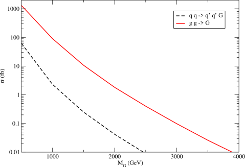
Figure 1: Cross section of KK graviton production with $M_{4}L=2.5$. Both the cross-section from gluon fusion $gg\rightarrow G$ and W boson fusion $qq\rightarrow q^{\prime}q^{\prime}WW\rightarrow q^{\prime}q^{\prime}G$ are shown.

2.4 Decay Rates/Width

The width of KK-graviton is dominated by the top quark (due to the large coupling to the right-handed top quark) and the TeV brane scalars (the Higgs boson and longitudinal W’s and Z’s). Other decay modes are suppressed by the volume factor $1/(\pi kr_{c})^{2}\sim 1/900$. The total width due to all four real scalar degrees of freedom is

$$\Gamma_{\rm Z_{L},W_{L},h}=\frac{1}{(M_{4}L)^{2}\mu_{TeV}^{2}}\frac{m_{grav}^{3}}{240\pi}=\left(\frac{2.5}{M_{4}L}\right)^{2}\frac{m_{grav}}{320}$$ (10)

For the $t_{R}$ quark contribution to the width, we find

$$\Gamma_{\rm top}=\frac{1}{(M_{4}L)^{2}\mu_{TeV}^{2}}\left(\frac{1+2\nu_{t,R}}{1-e^{-\pi kr_{c}(1+2\nu_{t,R})}}\frac{\int_{0}^{1}dy\ y^{2+2\nu_{t,R}}J_{2}(3.83y)}{J_{2}(3.83)}\right)^{2}\frac{3m_{grav}^{3}}{320\pi}$$ (11)

which is about $m_{grav}/320$ for $M_{4}L=2.5$ and $\nu_{t,R}=1$. The branching ratios are plotted in figure 2.

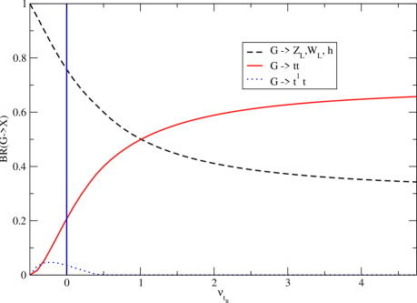
Figure 2: Branching Ratios for graviton decay to scalars and quarks as a function of the top-right localization parameter $\nu_{t,R}$. At $-0.5<\nu_{t,R}<-0.2$, the dominant decay is to the Higgs and longitudinal gauge bosons $Z_{L},W_{L}^{\pm}$. At $\nu_{t,R}>-0.2$, the dominant decay is to $t\bar{t}$. The decay to a zero-mode top and a KK anti-top is kinematically allowed in the range $-0.5<\nu_{t,R}<0.5$. The line at $\nu_{t,R}$ corresponds to the specific choice made in  [6].

For a range of possible $\nu_{t,R}$, the decay to a KK top and a zero-mode top will also be allowed. From equation (4), the mass of the KK top is approximately $(1+\nu_{t,R}/2)\pi\mu_{TeV}$; the mass will be less than the KK graviton mass $3.83\mu_{TeV}$ for $\nu_{t,R}<1/2$. Below this value, the decay width is

$$\Gamma_{t^{1}t}=\frac{1}{(M_{4}L)^{2}\mu_{TeV}^{2}}\left(\frac{2(1+2\nu_{t,R})}{1-\epsilon^{2\nu_{t,R}+1}}\right)\left(\int_{0}^{1}dyy^{\nu_{t,R}+5/2}\frac{J_{\nu_{t,R}-1/2}(x_{1}^{L}y)}{J_{\nu_{t,R}-1/2}(x_{1}^{L})}\frac{J_{2}(3.83y)}{|J_{2}(3.83)|}\right)^{2}\frac{3m_{grav}^{3}}{320\pi}\left|\frac{2p_{f}}{m_{grav}}\right|$$ (12)

where $p_{f}$ is the spatial momentum of either outgoing decay product. This kinematic factor vanishes when the zero mode top and KK top mass sum to the KK graviton mass, so the decay shuts off at a little below $\nu_{t,R}=1/2$.

Although for small $M_{4}L$ the widths become large, this is the most favorable limit for discovery, because the production rate also grows in this limit. In fact, the widths do not even become very large for small $M_{4}L$, and even for $M_{4}L=1$ and $\nu_{t,R}=2$, the width is only six percent of the KK graviton mass. This is distinctly different from the case when the Standard Model is on the brane and the graviton can decay to a wide array of light fermions. With the Standard Model fermions on the brane, at $M_{4}L$ less than about 2, the KK graviton cross-section flattens out and the tower of KK modes blur together, no longer appearing as individual resonances [4].

3 Discovery Reach

Before discussing the discovery reach of the KK-graviton, we first consider potential backgrounds. As discussed above, $gg\rightarrow G^{1}\rightarrow t\bar{t}$ is the dominant mode so $t\bar{t}$ production from the Standard Model is the chief background and is the one we consider in our discovery reach estimates below.

Another potential source of background could be KK gauge Bosons, which also decay into $t\bar{t}$ final states. The most important example is the KK-gluon, which has a much larger production cross-section and could therefore be one of the the major backgrounds through the KK-gluon $\rightarrow t\bar{t}$ channel. However, we expect the invariant masses of the two resonances should be quite different. With no brane kinetic terms for the gauge boson, the masses of the first KK gluon resonance and the first KK graviton resonance differ by a factor of 1.5 (this is also true for the masses of the first KK graviton and the second KK gluon), which is larger the width of the KK-gluon. Also, as we will discuss in section 4, the angular distribution of the decay products is different and should help distinguish the spin-1 and spin-2 modes. For these reasons, we have not included the effect of KK-gluon in our study of discovery reach.

The channel for graviton decay to scalars (i.e. Higgs and longitudinal W’s and Z’s) has a smaller branching ratio in the region $\nu_{t,R}\gtrsim 1$, $\sim 30\%$ in the model of Ref. [6]. On the other hand, it could be the dominant mode in the region $-1/2<\nu_{t,R}<1$. The existence of such a decay channel could be very important in distinguishing KK-graviton channel from KK-gluon production, since KK-gluon does not decay into such states. Since the size of this channel is somewhat model dependent, we will not take it into account in the following analysis. We expect it will enhance the discovery potential for the KK-graviton in a generic setup.

Note that an important difference between a KK-gluon and a heavy Higgs state, in addition to their spins, is the relative decay to weak gauge bosons. Both of them decay into $t\bar{t}$ as well as $WW$, $ZZ$. For the Higgs, due to the longitudinal enhancement and the fact that the Higgs mass is proportional to its self-coupling, decays into gauge bosons are dominant. However, there is no such enhancement for the KK-graviton and $t\bar{t}$ tends to be a somewhat larger channel.

The rate for KK graviton production as function of the mass of the KK-graviton is shown in Fig. 1. Comparing with the SM $t\bar{t}$ background, we obtain the reach for discovery, shown in Fig. 3. For $\nu_{t,R}=0$, the reach as a function of $M_{4}L$ is roughly parameterized by $m_{grav}=2.8TeV\times e^{-0.55(M_{4}L)+0.061(M_{4}L)^{2}}$, and for $\nu_{t,R}=10.0$, by $m_{grav}=3.86TeV\times e^{-0.45(M_{4}L)+0.040(M_{4}L)^{2}}$. There is no special significance to the form of this parameterization. We have assumed 100% efficient top reconstruction. The branching ratio to tops decreases with decreasing $\nu_{t,R}$, so we have plotted the reach for several possible values of $\nu_{t,R}$. The KK-graviton resonance is extremely narrow, even at small $M_{4}L$, which cuts down on the background. However, the narrow resonance will be smeared out by uncertainty in the measurement of the invariant mass of the KK resonance. Thus, even with a very narrow width, the resonance will have to contend with background events whose invariant mass is within a few percent of the graviton mass. We have estimated the effect of this uncertainty by taking the background to be all $t\bar{t}$ events within 3.0 % $m_{grav}$ of the graviton mass, i.e., we have we used the smeared width as the window in which we compare signal vs background. The smearing we have used $\sigma=E\times 3\%$ is a typical value for ATLAS ([12], Ch. 9).

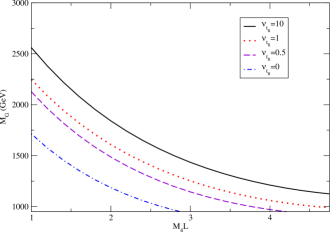
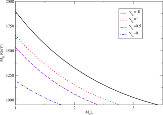
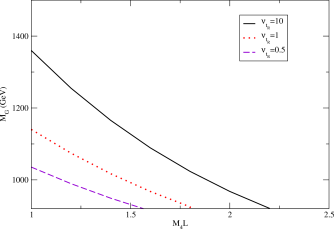
Figure 3: The $s/\sqrt{b}=5$ reach as a function of graviton mass and the parameter $(M_{4}L)$. From top to bottom, the reach is shown for 100%, 10%, and 1% efficient top identification. Different levels of top IR localization are shown, $\nu_{t,R}=10.0,1.0,0.5,0.0$. Larger $\nu_{t,R}$ corresponds to a more IR-localized $t_{R}$.

3.1 Energetic Top ID in $t\bar{t}$ final state

Realistically, we will have to include top identification efficiencies for both the signal and the background. Our signal significance, assuming the efficiency for signal and background are roughly the same, will scale down as the square root of the efficiency. Of course, any top identification method will also introduce fakes from other Standard Model processes, and these will effect the signal significance. A detailed study of these effects is beyond the scope of this paper. In this section, we will discuss new kinematical features of $t\bar{t}$ decaying from a heavy resonance, which will bring about uncertainties in top identification. We comment on possible ways of developing alternative methods of identifying tops in this type of processes. Due to such uncertainties and potential room for improvement, we present the KK-graviton discovery reach for a set of benchmark values of top identifcation efficiencies.

Studies focused on identifying SM $t\bar{t}$ produced near threshold typically yield a low efficiency [12], [13], [14], [15], [16]. For example, in the ATLAS study, the combined efficiency of the semi-leptonic and pure leptonic channel is about $10\%$ [14]. Since we are interested in a region which is far away from the $t\bar{t}$ production threshold, we expect the characteristics of the tops will be different. Top identification in this kinematical regime is critical to KK graviton discovery.

The simplest method for top identification would be to construct the invariant mass of the top quarks from their well separated decay products [11, 12, 13]. Doing this requires $\Delta R$, which measures the angle between the $b$ quark and lepton (for semileptonic decay) or the maximal angle with the jet (for purely hadronic decay), to be greater than 0.4 so that the final states are identified as separate jets and a reasonably accurate invariant mass can be calculated. In Figure 4, we show a Monte Carlo for the expected $\Delta R$ for various values of the KK graviton mass. We see that in all cases where we can hope to find the KK graviton resonance, a sizable fraction of the events have sufficiently large separation, which is very promising [19].

This method might well suffice for top identification in the mass regime for which discovery is possible. To enhance statistics, in addition to the conventional method, we can imagine other methods for top identification. In the case of a heavier KK-graviton, we expect a sizable amount of the event will have one or two top quarks highly collimated, especially if we use a somewhat larger cone size, for example 0.7 for $m_{grav}\gtrsim 2.5TeV$, see Fig. 4. If so, we expect they will show up in the form of one or two massive jets, which typically have a lepton in them. Without reliable top identification to distinguish it from a QCD jet, we will have to deal with a much bigger jet background that would make the collimated top quarks unobservable. One possibility is that we could use a massive jet algorithm, for example [17], so that all the decay products of each top that fall within the jet cone have a large invariant mass. However, QCD could also produce massive jets via off-shell partons and its contribution could be significant [18]. For this reason, an alternative method, based on the different substructure of top jets and QCD jets could be useful. Such substructure could be probed, for example, by using finer granularity on the tracks which would provide additional information on the substructure of the top-like objects. Given the importance of the energetic top signal, we consider further detailed study on the experimental viability of such a signature to be very worthwhile.

There could be room for improvement in the top identification efficiency. First of all, the top quarks produced from the KK resonance will have significantly different kinematics compared with the threshold production region considered in the studies [12], [13], [14], [15], [16]. For example, the top quarks produced from KK graviton decay will tend to be much harder ($p_{T}^{t}\sim 0.5m_{\rm reson}$), and therefore less trigger suppressed. On the other hand, large boosts will tend to make the top decay products more collimated. However, as can be seen from Figure 4, within the range of mass we are interested in, this does not represents a significant reduction in the signal rate.

Notice that our focus is on identifying $t\bar{t}$ resonance, rather than fully reconstructing all the decay products of top quark. Therefore, one could also explore alternative strategies, such as applying a looser definition of the top quark, including less focus on b-tagging and a relaxed W reconstruction condition. For highly boosted top quarks, one could also attempt to improve the efficiency by identifying the tops as massive fat jets with some substructure. Of course, all of these methods will introduce new backgrounds which need to be included in the analysis.

Since the top identification efficiency is uncertain, in figure 3 we have plotted the KK-graviton discovery reach for efficiencies of $1\%$ (the minimum expected), $10\%$ (as in the quoted studies), and $100\%$. We see that for $1\%$ efficiency, the reach is typically around $m_{\textrm{grav}}\sim$ 1 TeV. Results for any other efficiency could be obtained by scaling $s/\sqrt{b}$ by $\sqrt{\frac{\textrm{eff}_{1}}{\textrm{eff}_{2}}}$. Since the cross-section approximately satisfies $\sigma\propto(M_{4}L)^{-2}$, this can be compensated for by a rescaling of $M_{4}L\rightarrow M_{4}L\left(\frac{\textrm{eff}_{1}}{\textrm{eff}_{2}}\right)^{1/4}$. For example, a reach of $m_{\textrm{grav}}=2$ TeV at $M_{4}L=1.8$ with 100% efficient top identification corresponds to the same reach at $M_{4}L=1$ with 10% efficiency, as one can verify by inspection.

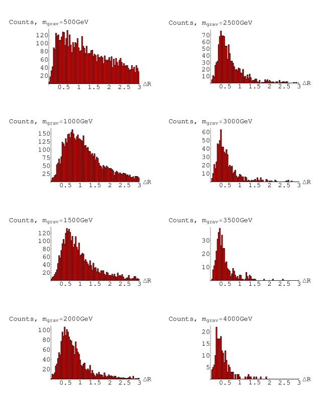
Figure 4: Distributions of $\Delta R$ of top decay products for various KK masses.

4 Spin measurement

The channel $q\bar{q}\rightarrow V\rightarrow{t\bar{t}}$ will have the characteristic distribution of $1+\cos^{2}\theta$ since it is dominated by the transverse mode of vector boson $V$. On the other hand, the KK-graviton, produced through gluon fusion, will have a $1-cos^{4}\theta$ dependence. This leads to a distinct difference from a spin-1 resonance in the cross-section near forward and backward scattering and could in principle allow one to rule out a spin-1 particle with $\mathcal{O}(100)$ reconstructed top pairs. A generic sample of 100 $t\bar{t}$ events, binned in 10 bins from $\cos\theta=-1$ to $\cos\theta=+1$, is shown in Figure 5. The $\chi^{2}/ndof$ for the spin-2,spin-1, and spin-0 distributions shown is 0.99, 3.7, and 2.1, respectively, where the number of degrees of freedom is $ndof=10$. The expected number of bins is shown for a spin-2, spin-1, or spin-0 resonance. The resolution is lower at near forward or backward scattering, requiring a cut on pseudo-rapidity $\eta>2.5$. We have taken this into account by conservatively assuming all gluons are as boosted as kinematically allowed, so we cut out events with $\eta>2.5-\ln 2$ in the graviton rest frame. As a result, some events have been cut from all three distributions in the two extreme bins. A spin-0 distribution is more difficult to rule out than a spin-1 distribution, and would require more events.

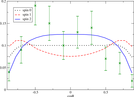
Figure 5: Generic Sample of 100 $gg\rightarrow G\rightarrow t\bar{t}$ events. The results of a Monte Carlo of 100 spin-2 events are shown on top of the expected results for a spin-0, spin-1, and spin-2 resonance. Events have been removed both from the expected curves and the Monte Carlo events if they are too close to forward or backward scattering to be likely to be observed (that is, if pseudo-rapidity $\eta>2.5-\ln 2$).

The fact that the cross-section $\sigma_{gg\rightarrow G\rightarrow t\bar{t}}$ vanishes at $\cos\theta=\pm 1$ follows from conservation of angular momentum. Of the five polarizations for the KK graviton, only the three with $L_{z}=\pm 2,0$ can be produced by the gluons. Moreover, the incoming and outgoing state must have total angular momentum $l=2$, so the KK graviton cannot decay to an s-wave top-pair, but instead must decay to a p-wave top pair. The only p-wave spherical harmonic that does not vanish along the z-axis is $Y_{10}$, so the spatial wave function cannot contribute to the value of $l_{z}$ and thus the tops cannot couple to the $L_{z}=\pm 2$ polarizations. Furthermore, the coupling $\bar{v}(p)\gamma^{\mu}u(p^{\prime})$ vanishes when the quarks have the same helicity, so there is no coupling to the $L_{z}=0$ polarization either. Thus the total cross-section vanishes along the z-axis, as shown in Figure 5.

Note that the fact that the KK-graviton has spin 2 could be used to our advantage in top identification – it may be possible to cut down on background by using the angular distribution of the tops to preferentially select the central region of phase space in figure 5.

5 Conclusion

We have considered the LHC signatures of a KK graviton within the context of RSI, when the top quarks are localized very near the TeV brane and the lighter quarks are localized near the Planck brane. We computed the cross-section for KK gravitons in this model and the discovery reach from $t\bar{t}$ pairs. We find that the KK graviton resonance is very narrow, its width being less than a few percent of its mass even for $M_{4}/k$ very close to 1, which is distinctly different from the case when all fermions are localized on the brane and there is a large number of possible decays for the graviton. The dominant production/decay mechanism is gluons $\rightarrow$ graviton $\rightarrow t\bar{t}$, and in this case the angular distribution of the cross-section is easier to distinguish from that of a spin-1 resonance than in models with fermions on the brane. The reason is that conservation of angular momentum forces the cross-section to vanish at forward and backward scattering for a spin-2 resonance, whereas the cross-section increases at forward and backward scattering for a spin-1 resonance. We find that the spin-2 distribution can be resolved with $\sim 100$ events. In on-the-brane models, the dominant production/decay mechanism is fermions $\rightarrow$ graviton $\rightarrow$ fermions, and the spin-2 nature of the graviton is not as obvious. In other models, where the left handed quark doublet of the third generation is largely composite, both the rate of KK-graviton production and its branching ratio to top and bottom quarks could be larger. Thus KK-graviton phenomenology in these models deserves further study.

We find that the collider reach for detection is $m_{grav}\lesssim 1.7TeV$, and depends on the AdS curvature scale. Detecting the graviton at the limits of the collider reach depends on efficient reconstruction of the top decay products, and further work is necessary to determine how efficiently this can be done in practice. Because the tops result from the decay of a very massive graviton, they will be highly boosted and thus their decay products come out in a narrow cone (0.4 $\lesssim\delta R\lesssim 2.0$, depending on the KK graviton mass).

Note Added

Shortly after this work was submitted, there appeared the closely related work [20], focusing on KK graviton decays to W’s, and arguing that a slightly lower limit on $M_{4}L$ is allowed than that considered here.

Appendix A Goldstone Boson Equivalence on the Brane

The coupling between the W bosons and the graviton is difficult to calculate in the 5d theory. A precise calculation would involve writing down the 5d equations of motion for the gauge fields (which have no bulk mass term), writing down the symmetry-breaking Higgs terms on the TeV brane, and solving for the wavefunctions and mass eigenmodes satisfying the modified boundary conditions. Then, these would be integrated against the graviton wavefunction. The rough picture for the 5d wavefunctions is that, before symmetry-breaking, the gauge bosons start out with flat wavefunctions and the Higgs starts out with a delta function wavefunction on the brane. After symmetry-breaking, the gauge bosons eat a Higgs, and their wavefunctions are still mostly flat in the bulk but dip sharply near the brane.

Figure 6: When the Higgs gets a vev, the boundary conditions for the wavefunction of the W boson are modified, and the wavefunction dips down near the TeV brane.

A much easier and more transparent method is to go directly to the effective KK theory before including the effects of symmetry-breaking. Then, the W bosons pick up a mass from the usual Higgs mechanism in 4d, and their couplings are determined from the Higgs couplings by the usual Goldstone boson equivalence theorem, which states

$$\epsilon_{\mu_{1}}\epsilon_{\mu_{2}}\dots\epsilon_{\mu_{n}}\Gamma^{\mu_{1}\mu_{2}\dots\mu_{n}}=\Gamma$$ (13)

where $\Gamma^{\mu_{1}\mu_{2}\dots\mu_{n}}$ is the vertex for $n$ W bosons, $\epsilon^{\mu_{i}}$ are the longitudinal polarization vectors, and $\Gamma$ is the vertex for $n$ Higgses. This can be seen directly at the level of the lagrangian as well. The Higgs kinetic and interaction term are

$$\mathcal{L}\supset(\partial H)^{2}+c_{ssG}\partial_{\mu}H\partial_{\nu}Hh^{\mu\nu}$$ (14)

where $c_{ssG}$ is calculated using only the graviton wavefunction. Gauge invariance then constrains the W interaction terms to arise by promoting coordinate derivatives to covariant derivatives:

$$L\supset\left((\partial_{\mu}-i\frac{g_{5}\psi(\pi)}{2}W_{\mu})H\right)^{2}+c_{ssG}\left(\partial_{\mu}H-i\frac{g_{5}\psi(\pi)}{2}W_{\mu}H\right)\left(\partial_{\nu}H-i\frac{g_{5}\psi(\pi)}{2}W_{\nu}H\right)h^{\mu\nu}$$ (15)

The factor $\psi(\pi)$ is the W wavefunction evaluated on the TeV brane. We can absorb this factor into the coupling:

$$g_{4}=g_{5}\psi(\pi)$$ (16)

If $v=\langle H\rangle$ is the Higgs vev, then the mass term for W and the coupling to the graviton can be written

$$\mathcal{L} \supset \left(\frac{g_{4}v}{2}\right)^{2}W^{2}+c_{ssG}\left(\frac{g_{4}v}{2}\right)^{2}W_{\mu}W_{\nu}h^{\mu\nu}$$ (17)

$$c_{ssG} = \frac{2}{(M_{4}L)\mu_{TeV}}$$ (18)

so it is manifest that the coupling of the W to the graviton is just $c_{ssG}$ times the mass-squared. At high energies, the longitudinal polarization $\epsilon^{\mu}=\frac{p^{\mu}}{m_{W}}+\mathcal{O}\left(\frac{m_{w}}{E_{p}}\right)$, so the W coupling to the graviton acts exactly as a Higgs.

Appendix B Loops

In principle, there are contributions from top loops that could enhance the production cross section for KK gravitons. These contributions could be relevant because the top coupling to the KK graviton is much stronger than the gluon coupling, which is suppressed by a volume factor $\pi kr_{c}$.

The KK description of RS is a (Wilsonian) effective field theory defined below the scale $N\mu_{TeV}$. We can write the relevant interactions very schematically as

$$L\supset\frac{c_{1}}{N\mu_{TeV}}F_{\mu\rho}F_{\nu}^{\rho}h^{\mu\nu}+\frac{c_{2}}{N\nu_{TeV}}h^{\mu\nu}i\psi^{\dagger}\bar{\sigma}_{\mu}D_{\nu}\psi$$ (19)

To make predictions, we would in principle match this EFT to a UV description at some matching scale $\mu_{match}$, and then we would use the RG running of $c_{1}$ and $c_{2}$ to make predictions at any other scale (and we would also have other $c_{i}$’s for higher order interactions).

However, in our case we do not have an accessible UV description. All we have is a tree-level matching condition at an unknown matching scale, assumed to be of order the cutoff. This seems to set a limit on the precision of our predictions. For instance, consider the amplitude for two gluons and a KK graviton, which is schematically given as

$$A=\frac{p^{2}}{N\mu_{TeV}}\left(c_{1}(\mu)+\frac{g^{2}c_{2}(\mu)}{16\pi^{2}}\right)$$ (20)

where $\mu$ is the relevant scale. Clearly if the $c_{2}$ contribution is much smaller than the contribution from $c_{1}$, then we should ignore it. However, if

$$c_{1}(\mu_{match})\ll\frac{g^{2}c_{2}}{16\pi^{2}}$$ (21)

then it would be very unnatural to ignore the loop correction from $c_{2}$, because even if $c_{1}$ is very small at some scale, it will be regenerated by $c_{2}$. In our case this is especially true, because we do not even know $\mu_{match}$. Thus the loop contribution sets a natural lower bound on $c_{1}$. Now if

$$c_{1}(\mu_{match})\gtrsim\frac{g^{2}c_{2}}{16\pi^{2}}$$ (22)

then we can include the loop correction, but it does not seem to make our analysis more precise. This is because we only know $c_{1}$ at tree level, while there are unknown corrections to it from the one-loop matching at $\mu_{match}$ and from the RG running of the coefficient $c_{1}$, and these are of the same order as the loop.

In our case, we found that the top loop contribution is smaller than the tree level gluon contribution, although they are roughly of the same order of magnitude. This can be viewed as an additional source of error in our analysis.

Appendix C Analytic Cross-section Estimates

C.1 W Boson Fusion

We are interested in approximating the cross-section for $q_{1}q_{2}\rightarrow q^{\prime}_{1}q^{\prime}_{2}WW\rightarrow q^{\prime}_{1}q^{\prime}_{2}G$, where $G$ is a graviton. The fermion-fermion-W vertex is

$$\frac{g_{w}}{\sqrt{2}}\bar{u}(q)\gamma^{\mu}\left(\frac{1-\gamma^{5}}{2}\right)u(q^{\prime})W_{\mu}$$

and the WWG vertex is

$$\epsilon^{\mu\nu}W_{\mu}W_{\nu}m_{w}^{2}c_{ssG}$$

We work in the rest frame of the incoming quarks, so their 4-momentum is

$$q_{1}+q_{2}=(2E,0,0,0)$$

It is convenient to parameterize the outgoing quark energies and the difference in their directions by

$$E_{1}^{\prime} = (1-\eta)E$$

$$E_{2}^{\prime} = (1-\zeta)E$$

$$\cos\theta = -\hat{p}^{\prime}_{1}\cdot\hat{p}^{\prime}_{2}$$ (23)

Denoting the graviton momentum as $k^{\mu}$, its 3-momentum is

$$\vec{l}^{2} = (\vec{p}^{\prime}_{1}+\vec{p}^{\prime}_{2})^{2}=E_{g}^{2}-m_{g}^{2}$$ (24)

and after some algebra, we find

$$\cos\theta = 1-\frac{2(\eta\zeta-m_{g}^{2}/4E^{2})}{(1-\eta)(1-\zeta)}$$ (25)

The kinematic bounds on $\eta$ and $\zeta$ are therefore $\eta\zeta>m_{g}^{2}/4E^{2}$ and $\eta+\zeta<1+m_{g}^{2}/4E^{2}$. We parameterize the outgoing quark directions by

$$\hat{q}^{\prime}_{1} = (\cos\alpha\cos\beta,\sin\alpha,-\sin\beta\cos\alpha)$$

$$\hat{q}^{\prime}_{2} = -\hat{q}^{\prime}_{1}(\alpha\rightarrow\alpha-\theta)$$ (26)

We denote the W momenta as $k_{1}=q_{1}-q^{\prime}_{1}$ and $k_{2}=q_{2}-q^{\prime}_{2}$. The matrix element squared, averaged over initial spins and summed over final ones, is therefore

$$|M|^{2} = \frac{g^{4}}{2}(q_{1\mu}q^{\prime}_{1\mu^{\prime}}-q_{1}\cdot q^{\prime}_{1}g_{\mu\mu^{\prime}}+q_{1\mu^{\prime}}q^{\prime}_{1\mu})(q_{2\nu}q^{\prime}_{2\nu^{\prime}}-q_{2}\cdot q^{\prime}_{2}g_{\nu\nu^{\prime}}+q_{2\nu^{\prime}}q^{\prime}_{2\nu})$$ (27)

$$\times \left(\frac{1}{k_{1}^{2}-m_{w}^{2}}\right)^{2}\left(\frac{1}{k_{2}^{2}-m_{w}^{2}}\right)^{2}D_{\mu\nu;\mu^{\prime}\nu^{\prime}}$$

where $D_{\mu\nu;\mu^{\prime}\nu^{\prime}}$ is the sum over graviton polarizations, equal to the numerator of the graviton propagator:

$$D_{\mu\nu;\mu^{\prime}\nu^{\prime}} = \frac{1}{2}\left(G_{\mu\mu^{\prime}}G_{\nu\nu^{\prime}}+G_{\mu\nu^{\prime}}G_{\mu^{\prime}\nu}-\frac{2}{3}G_{\mu\mu^{\prime}}G_{\nu\nu^{\prime}}\right)$$

$$G_{\mu\nu} = g_{\mu\nu}-\frac{k_{\mu}k_{\nu}}{m_{g}^{2}}$$ (28)

The W propagators can be simplified:

$$k_{1}^{2}-m_{w}^{2} = 2E^{2}(1-\eta)\left(x+\cos\alpha\sin\beta\right)$$

$$k_{2}^{2}-m_{w}^{2} = 2E^{2}(1-\zeta)\left(y+\cos(\alpha-\theta)\sin\beta\right)$$

$$x = 1+\frac{m_{w}^{2}}{2E^{2}(1-\eta)}$$

$$y = 1+\frac{m_{w}^{2}}{2E^{2}(1-\zeta)}$$ (29)

When $E\gg m_{w}$, there is a near-divergence in the W propagators that is cut off by the W mass, and the dominant contribution to the cross-section comes from $\theta\sim 0$ and $\cos\alpha\sin\beta=-1$. We can expand $\alpha$ around $\pi$ and $\beta$ around $\pi/2$:

$$\alpha = \pi-\nu$$

$$\beta = \pi/2-\epsilon$$

$$\cos\alpha \sim -1+\frac{1}{2}\nu^{2}$$

$$\sin\beta \sim 1-\frac{1}{2}\epsilon^{2}$$

$$\cos(\alpha-\theta) \sim -1+\frac{1}{2}(\nu+\theta)^{2}$$ (30)

We are left with an expression that is still relatively complicated. We start by focusing on the $\nu-$,$\epsilon-$, and $\theta$-dependence:

$$d\sigma \propto J(\theta)=16\int d\nu d\epsilon\left(\frac{1+\mathcal{O}(\nu^{2},\epsilon^{2})}{2(x-1)+(\nu^{2}+\epsilon^{2})}\right)^{2}\left(\frac{1+\mathcal{O}(\nu^{2},\epsilon^{2})}{2(y-1)+((\nu+\theta)^{2}+\epsilon^{2})}\right)^{2}$$ (31)

The leading order term can be evaluated exactly. The $\mathcal{O}(\nu^{2},\epsilon^{2})$ terms diverge individually (of course, they are part of an expansion of $\cos$ so they do not diverge if summed up) so we will drop them. They would lead to a partial cancellation, since we are essentially approximating $\cos\nu=1-\frac{1}{2}\nu^{2}+\dots$ by $\cos\nu=1$ near $\nu=0$ in the numerator. This amounts to keeping the angular dependence of only the $(k_{1}^{2}-m_{w}^{2})^{-2}(k_{2}^{2}-m_{w}^{2})^{-2}$ piece in the amplitude. These are the terms responsible for the divergence (in the limit $E\gg m_{w}$) when the W’s are collinear. Consequently, the remaining terms get their dominant contribution from $\theta=0$, so we approximate $J\propto\delta(\theta^{2})$, with proportionality contant given by

$$\int d\theta^{2}J = 2\int\theta d\theta J=\frac{1}{\pi}\int d^{2}\theta J$$ (32)

$$= \frac{16}{\pi}\int\frac{d\nu d\epsilon}{(2(x-1)+(\nu^{2}+\epsilon^{2}))^{2}}\int\frac{d\theta_{x}d\theta_{y}}{(2(y-1)+((\nu+\theta_{x})^{2}+(\epsilon+\theta_{y})^{2})^{2}}$$

$$= \frac{4\pi}{(x-1)(y-1)}$$

So, in this approximation,

$$J = \int d\alpha d\cos\beta\left(\frac{1}{k_{1}^{2}-m_{w}^{2}}\right)^{2}\left(\frac{1}{k_{2}^{2}-m_{w}^{2}}\right)^{2}$$ (33)

$$= \frac{4\pi}{(x-1)(y-1)}\delta(\theta^{2})$$

The rest of $d\sigma$ can now be evaluated at this level of approximation by a straightforward but tedious computation, since $\alpha=\pi,\beta=\pi/2$ and $\theta=0$:

$$(k_{1}^{2}-m_{w}^{2})^{2}(k_{2}^{2}-m_{w}^{2})d\sigma = \frac{16}{3}E^{4}(1-\zeta)(1-\eta)(1-\zeta\eta+\zeta^{2}\eta^{2})\times\left(g^{4}2^{-10}\pi^{-4}m_{w}^{4}c_{ssG}^{2}\right)$$ (34)

Putting everything together and using $\theta^{2}=\frac{4(\eta\zeta-m_{g}^{2}/4E^{2})}{(1-\eta)(1-\zeta)}$ from above, we get

$$\sigma = \int_{m_{g}^{2}/4E^{2}}^{1}d\eta\int_{m_{g}^{2}/4E^{2}}^{1+(m_{g}^{2}/4E^{2})-\eta}d\zeta\frac{g^{4}}{2^{12}\pi^{4}}\frac{16\pi}{3}\frac{1}{m_{w}^{4}}(1-\zeta\eta+\zeta^{2}\eta^{2})\delta(\frac{4(\eta\zeta-m_{g}^{2}/4E^{2})}{(1-\eta)(1-\zeta)}m_{w}^{4}c_{ssG}^{2}$$ (35)

$$= \frac{g^{4}}{(3)2^{10}\pi^{3}}c_{ssG}^{2}(1-\hat{\tau}+\hat{\tau}^{2})\left((1+\hat{\tau})\log\left(\frac{1}{\hat{\tau}}\right)-2(1-\hat{\tau})\right)$$

where $\hat{\tau}=\frac{m_{g}^{2}}{4E^{2}}=\frac{m_{g}^{2}}{\hat{s}}$. This contains the usual luminosity function $-((1+\hat{\tau})\log(\hat{\tau})+2(1-\hat{\tau}))$ for effective longitudinal W’s, as well as an additional piece from the spin structure of the resonance. We convolve this with the fermion luminosity function

$$\frac{\partial\mathcal{L}}{\partial\tau} = 2\int_{\tau}^{1}\frac{dx}{x}f_{+}(x)f_{-}(\tau/x)d\tau$$ (36)

where $f_{+}$ is the sum of pdfs for the positively charged fermions and $f_{-}$ is for the negatively charged ones. The cross-section is then

$$\int_{\hat{\tau}}^{1}\frac{\partial\mathcal{L}}{\partial\tau}(\tau)\sigma(\tau)$$

To evaluate this numerically, we used the CTEQ5M parton distribution functions in their Mathematica distribution package[10]. We compare this with the results of the Monte Carlo integration below:

$m_{grav}$ (TeV)	$\sigma_{est}$ (fb)	$\sigma_{prog}$ (fb)	$m_{grav}$ (TeV)	$\sigma_{est}$ (fb)	$\sigma_{prog}$ (fb)
0.5	47	62	2.5	0.012	0.0089
1.0	2.3	2.3	3.0	0.0029	0.0022
1.5	0.29	0.25	3.5	0.00079	0.00056
2.0	0.053	0.042	4.0	0.00022	0.00016

For the convenience of the reader, we found that the CTEQ5M pdf’s at an energy scale $Q=200TeV$ can be parameterized by

$$xg(x) = \frac{1.549e^{-3.113x^{1/3}}(1-x)^{5.448}}{x^{0.5270}}$$

$$xu(x) = \frac{0.02596e^{7.667\sqrt{x}}(1-x)^{7.273}}{x^{0.6125}}$$

$$xd(x) = \frac{0.04735e^{4.309\sqrt{x}}(1-x)^{6.203}}{x^{0.5267}}$$

C.2 Gluon Fusion

Since the gluon fusion is a two-to-two decay, it can be evaluated exactly. The amplitude is

$$\mathcal{M} = T_{gluon}^{\mu\nu}D_{\mu\nu;\mu^{\prime}\nu^{\prime}}T^{\mu^{\prime}\nu^{\prime}}_{top}$$ (37)

This implies that the cross-section is

$$\frac{d\sigma}{d\cos\theta} = \frac{5}{64}\frac{m_{g}^{4}}{\hat{s}}(1-\cos^{4}\theta)c_{AAG}^{2}\frac{m_{g}^{-3}\Gamma_{t\bar{t}}}{\left(\frac{\hat{s}}{m_{g}^{2}}-1\right)^{2}+\frac{\Gamma_{\rm tot}^{2}}{m_{g}^{2}}}$$ (38)

Integrating over $\cos\theta$, we find

$$\sigma = \frac{1}{8}\frac{\tau}{\hat{\tau}}\left(\frac{0.47}{(35)(2.5)(m_{g}/3.83)}\right)^{2}\frac{m_{g}\Gamma_{t\bar{t}}}{\left(\frac{\hat{\tau}}{\tau}-1\right)^{2}+\frac{\Gamma^{2}}{m_{g}^{2}}}$$ (39)

To get the full cross-section, we convolve this with the gluon luminosity function:

$$\sigma_{tot} = \int_{\hat{\tau}}^{1}\frac{\partial\mathcal{L}}{\partial\tau}\sigma(\hat{\tau},\tau)d\tau$$ (40)

Comparison with the Monte Carlo integration is shown below (setting $\Gamma_{t\bar{t}}=\Gamma_{\rm tot}$, so this calculates the total graviton production cross-section, without the branching ratio of subsequent decay to tops):

$m_{grav}$ (TeV)	$\sigma_{est}$ (fb)	$\sigma_{prog}$ (fb)	$m_{grav}$ (TeV)	$\sigma_{est}$ (fb)	$\sigma_{prog}$ (fb)
0.5	2500	1300	2.5	0.32	0.40
1.0	85	91	3.0	0.078	0.098
1.5	9.0	11.	3.5	0.021	0.026
2.0	1.5	1.8	4.0	0.0061	0.0077

References

- [1] L. Randall and R. Sundrum, Phys. Rev. Lett. 83, 3370 (1999) [arXiv:hep-ph/9905221]. L. Randall and R. Sundrum, Phys. Rev. Lett. 83, 4690 (1999) [arXiv:hep-th/9906064].
- [2] H. Davoudiasl, J. L. Hewett and T. G. Rizzo, Phys. Rev. Lett. 84, 2080 (2000) [arXiv:hep-ph/9909255].
- [3] H. Davoudiasl, Int. J. Mod. Phys. A 15, 2613 (2000) [arXiv:hep-ph/0001248].
- [4] H. Davoudiasl, J. L. Hewett and T. G. Rizzo, Phys. Rev. D 63, 075004 (2001) [arXiv:hep-ph/0006041].
- [5] A. Pomarol, Phys. Lett. B 486, 153 (2000) [arXiv:hep-ph/9911294].
- [6] K. Agashe, A. Delgado, M. J. May and R. Sundrum, JHEP 0308, 050 (2003) [arXiv:hep-ph/0308036].
- [7] K. Agashe, A. Belyaev, T. Krupovnickas, G. Perez and J. Virzi, arXiv:hep-ph/0612015. B. Lillie, L. Randall, L.-T. Wang, to appear
- [8] W. M. Yao et al. [Particle Data Group], J. Phys. G 33, 1 (2006).
- [9] R. N. Cahn, Nucl. Phys. B 255, 341 (1985)
- [10] J. Pumplin, D. R. Stump, J. Huston, H. L. Lai, P. Nadolsky and W. K. Tung, JHEP 0207, 012 (2002) [arXiv:hep-ph/0201195].
- [11] B. Abbott et al. [D0 Collaboration], Phys. Rev. D 58, 052001 (1998) [arXiv:hep-ex/9801025]. F. Abe et al. [CDF Collaboration], Phys. Rev. Lett. 80, 2767 (1998) [arXiv:hep-ex/9801014].
-
[12]
“ATLAS: Detector and physics performance technical design report. Volume
1,”
CERN-LHCC-99-14.
“ATLAS detector and physics performance. Technical design report. Vol. 2,” CERN-LHCC-99-15 -
[13]
CMS Techinical Design Report V.1., CERN-LHCC-2006-001,
CMS Techinical Design Report V.2., CERN-LHCC-2006-021 - [14] F. Hubaut, E. Monnier, P. Pralavorio, K. Smolek and V. Simak, Eur. Phys. J. C 44S2, 13 (2005) [arXiv:hep-ex/0508061].
- [15] M. Baarmand, H. Mermerkaya and I. Vodopianov,
- [16] L. March, E. Ros and B. Salvachua, phys-pub-2006-002
- [17] J. M. Butterworth, B. E. Cox and J. R. Forshaw, Phys. Rev. D 65, 096014 (2002) [arXiv:hep-ph/0201098].
- [18] J. M. Campbell, J. W. Huston and W. J. Stirling, arXiv:hep-ph/0611148.
- [19] V. Barger, T. Han and D. G. E. Walker, arXiv:hep-ph/0612016.
- [20] K. Agashe, H. Davoudiasl, G. Perez and A. Soni, “Warped Gravitons at the LHC and Beyond,” arXiv:hep-ph/0701186.