Inflaton Fragmentation After $\lambda\phi^{4}$ Inflation

Abstract

We use lattice simulations to examine the detailed dynamics of inflaton fragmentation during and after preheating in $\lambda\phi^{4}$ chaotic inflation. The dynamics are qualitatively similar to preheating after $m^{2}\phi^{2}$ inflation, involving the exponential growth and subsequent expansion and collision of bubble-like inhomogeneities of the inflaton and other scalar fields. During this stage fluctuations of the fields become strongly non-Gaussian. In the quartic theory, the conformal nature of the theory allows us to extend our simulations to much greater times than is possible for the quadratic model. With these longer simulations we have been able to determine the time scale on which Gaussianity is restored, which occurs after a time on the order of a thousand inflaton oscillations.

I Introduction

After inflation the energy density of the nearly homogeneous inflaton field decays into fluctuations of the inflaton and other fields. In many simple models of inflation this process begins with an exponentially rapid stage of decay that produces highly inhomogeneous, nonthermal field fluctuations. In large field chaotic inflation models preheating occurs via parametric resonance, which has been analyzed both analytically (see e.g. KLS ) and numerically KT . This preheating stage is followed by a short, violent transition that leads to a regime of Kolmogorov turbulence MT .

In bubbles this transition stage was studied for a model with inflaton potential $V=(1/2)m^{2}\phi^{2}$. It was found there that parametric resonance leads to growth of fluctuations in the peaks of the initial random gaussian field, giving rise to a quasi-stable standing wave pattern of bubbles and nodes. This growth continues until backreaction makes parametric resonance inefficient, after which these bubbles expand and collide, thus bringing the entire space into the strongly inhomogeneous regime. It was found there that the fluctuations produced during preheating are strongly non-Gaussian, and that this non-Gaussianity persists long after the end of parametric resonance.

For technical reasons discussed below, the simulations performed in bubbles could not be continued long enough to determine the ultimate fate of these non-Gaussian perturbations. In this paper we explore these same questions in a quartic model with an inflaton potential $V=(1/4)\lambda\phi^{4}$. In this model it is possible to run the simulations to much later times and we were thus able to see the field statistics return to Gaussianity.

In section II we describe the model we are using and our numerical simulations. In section III we present the results of our simulations and discuss their implications.

II The Model

We consider the potential

$$V={1\over 4}\lambda\phi^{4}+{1\over 2}g^{2}\phi^{2}\chi^{2}$$ (1)

where $\phi$ is the inflaton and $\chi$ is another scalar field that is coupled to it. We use LATTICEEASY FT to solve the classical equations of motion for the two fields

$$\ddot{\phi}+3H\dot{\phi}-{1\over a^{2}}\nabla^{2}\phi+\left(\lambda\phi^{2}+g^{2}\chi^{2}\right)\phi = 0$$ (2)

$$\ddot{\chi}+3H\dot{\chi}-{1\over a^{2}}\nabla^{2}\chi+g^{2}\phi^{2}\chi = 0.$$ (3)

Oscillations of the zeromode of $\phi$ after inflation lead to parametrically resonant amplification of modes of $\chi$ within certain resonance bands. These amplified modes of $\chi$ in turn excite fluctuations of $\phi$.

LATTICEEASY uses a comoving grid, meaning the wavelength of produced fluctuations remains constant in program coordinates. In a quadratic model this comoving growth causes a problem for compuater simulations because the physical wavelength $m^{-1}$ at which modes are preferentially produced shrinks in these comoving variables. As the universe expands the grid spacing needs to remain small enough to accurately capture this physical length scale. Once the universe has expanded enough to violate this criterion, it is no longer possible to continue the simulation with any accuracy.

In the quartic model, however, the parameters $\lambda$ and $g$ are unitless and there is no fixed physical length scale in the problem. By defining a new set of variables $\phi_{pr}\equiv\phi/a$ and $\tau\equiv at$ the equations of motion can be recast as

$${\phi_{pr}^{\prime\prime}}-\nabla^{2}\phi_{pr}+\left(\lambda\phi_{pr}^{2}+g^{2}\chi_{pr}^{2}\right)\phi_{pr}+\Delta = 0$$ (4)

$${\chi_{pr}^{\prime\prime}}-\nabla^{2}\chi_{pr}+g^{2}\phi_{pr}^{2}\chi_{pr}+\Delta = 0$$ (5)

where primes represent differentiation with respect to $\tau$ and $\Delta$ represents derivatives of the scale factor that vanish for a radiation equation of state, an approximation that is very accurate for this model. In other words we can scale expansion out of the equations, and can thus simulate to much later times than would be possible for a quadratic model.

The simulations shown in this paper were done on a three dimensional grid of $128^{3}$ or $256^{3}$ gridpoints. The simulations start at the end of inflation when the mean value of the inflaton is $\phi_{0}=0.342M_{p}$. Times are reported in units of $1/(\sqrt{\lambda}\phi_{0})$ and field values are reported in units of $\phi_{0}$. All of the results shown in this paper are for $\lambda=9\times 10^{-14}$ and $g^{2}/\lambda=200$.

III Inflaton Fragmentation: Results and Conclusions

Figures 2 and 2 show the growth of fluctuations of the fields $\phi$ and $\chi$. The information in these plots is well known. The field $\chi$ grows exponentially. Some time after the growth of $\chi$ starts fluctuations of the field $\phi$ begins growing with twice the exponent of $\chi$. These plots are included here primarily as a reference for seeing where in the process of preheating the fields are at each of the times shown in the plots below.

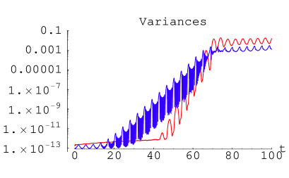
Figure 1: Variances of the fields $\phi$ (red) and $\chi$ (blue). (For black and white viewing, $\chi$ begins growing earlier; $\phi$ begins later but quickly catches up to $\chi$.)

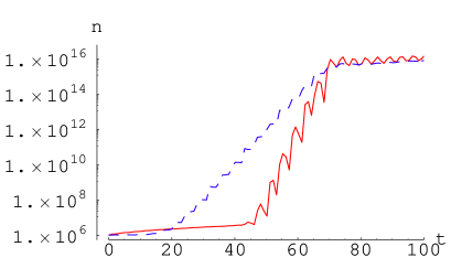
Figure 2: Number density for $\phi$ (red, solid) and $\chi$ (blue, dashed).

Figure 3 shows the growth of fluctuations of the $\chi$ field during preheating. For clarity the figures show values only on a one dimensional slice through the lattice. The initial conditions used for the model are gaussian random fluctuations with expectation values

$$\langle|\phi_{k}|^{2}\rangle={1\over 2\sqrt{k^{2}+m_{eff}^{2}}},$$ (6)

intended to simulate quantum vacuum fluctuations KT ; PS . See the LATTICEEASY documentation latticeeasyweb for more details. As parametric resonance begins fluctuations of the field begin to grow exponentially. Note that the vertical scale on the different frames of 3 is not constant. Since parametric resonance only excites modes with momenta below a certain cutoff ($k^{*}\sim(g^{2}\lambda)^{1/4}\phi_{0}$ GKLS ), the short wavelength fluctuations rapidly become insignificant. The longer wavelength modes, however, remain almost entirely unchanged except for their overall scale. In other words the spatial distribution of the fluctuations produced during preheating simply mimics the spatial distribution of the infrared modes of $\chi$ that were present before preheating.

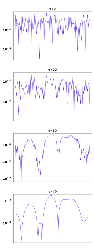
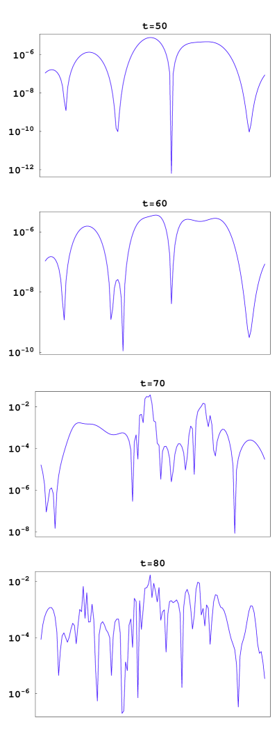
Figure 3: Values of the field $\chi$ on a 1D slice through the lattice.

Fluctuations of $\phi$ are not produced until later, but when they appear they grow due to interactions with the amplified $\chi$ fluctuations, so the peaks of $\delta\phi$ mostly correspond to the peaks of the initial random gaussian field $\chi$. Figure 4 shows a snapshot of $\phi$ and $\chi$ fluctuations shortly after the $\phi$ fluctuations have started to grow. The fluctuations of $\phi$ are for the most part in the same places as the fluctuations of $\chi$; the correlation between $\delta\phi^{2}$ and $\delta\chi^{2}$ in this plot is 0.72. However, the oscillation frequencies are different for the two fields so the fluctuations are in general not in phase, as can be seen in the plot.

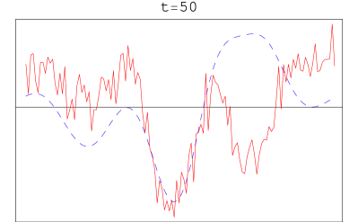
Figure 4: Values of field fluctuations $\delta\phi$ (red, solid) and $\delta\chi$ (blue, dashed) on a 1D slice through the lattice. Because the scale of $\delta\chi$ is much larger than $\delta\phi$ at the time shown, fluctuations of both fields are normalized to the same standard deviation.

Finally, we considered the field statistics for these field fluctuations. It is known that fluctuations produced during preheating are non-Gaussian (see e.g. KLS ). We measure the Gaussianity of the fields through the kurtosis, $3\langle f^{2}\rangle^{2}/\langle f^{4}\rangle$. It is a necessary but not sufficient condition for Gaussianity that this quantity be equal to one. Figure 5 shows the evolution of this quantity for fields $\phi$ and $\chi$. As noted in bubbles the fluctuations become non-Gaussian during preheating and begin slowly tending towards Gaussianity thereafter. We see here that Gaussianity is restored after a time of order of a thousand inflaton oscillations.

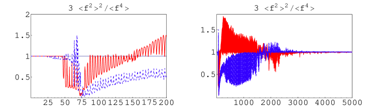
Figure 5: Kurtosis for the fields $\phi$ (red, solid) and $\chi$ (blue, dashed). The plot on the left shows the development of non-Gaussianity during preheating. The plot on the right shows a much larger time scale on which the return to Gaussianity can be seen.

We can understand this timing with a rough analytical estimate. Perturbatively the time scale for rescattering is given by $t_{r}\sim 1/(n\sigma)$ where $n$ and $\sigma$ are the number density and scattering cross sections for the gas of particles. The cross section can be estimated as $\sigma\sim g^{2}/k^{*2}$, where $k^{*}\sim(g^{2}\lambda)^{1/4}\phi_{0}$ is the typical particle momentum produced during preheating. To estimate the number density we can take $n\sim\rho/k^{*}\sim g^{2}<\phi^{2}><\chi^{2}>/k^{*}$. Putting all of this together

$$\sqrt{\lambda}\phi_{0}t_{r}\sim{1\over(g^{2}/\lambda)^{5/4}\langle\left(\phi/\phi_{0}\right)^{2}\rangle\langle\left(\chi/\phi_{0}\right)^{2}\rangle}.$$ (7)

Shortly after preheating the variances $\langle\left(\phi/\phi_{0}\right)^{2}\rangle$ and $\langle\left(\chi/\phi_{0}\right)^{2}\rangle$ are both approximately $10^{-3}$, so the rescattering time is of order

$$\sqrt{\lambda}\phi_{0}t_{r}\sim{1\over(200)^{5/4}10^{-6}}\sim 1000.$$ (8)

In other words the time that we found is required to restore Gaussianity has the expected order of magnitude.

In a lattice simulation all classical dynamics are automatically taken into account, so the Gaussianity of the fields is irrelevant to the accuracy of the simulation. While lattice simulations are excellent for describing preheating and the evolution shortly afterwards, they can not be extended to time scales long enough to describe the stages of turbulence and thermalization. Many approximation techniques are thus employed to describe these epochs (see e.g. MT and references therein), and for these it is often important to know the field statistics. Our results suggest that techniques that assume Gaussianity should not be employed immediately after preheating, but they also suggest that it can be possible to extend lattice simulations long enough to get through the non-Gaussian stage and thus overlap with the subsequent period that can be well described in other ways.

We would like to thank Lev Kofman for useful discussions and advice. This work was supported by NSF grant PHY-0456631.

References

- (1) L. A. Kofman, A. D. Linde and A. A. Starobinsky, Phys. Rev. Lett. 73, 3195 (1994); Phys. Rev. D 56, 3258 (1997).
- (2) S. Y. Khlebnikov and I. I. Tkachev, Phys. Rev. Lett. 77, 219 (1996) [arXiv:hep-ph/9603378].
- (3) R. Micha and I. I. Tkachev, Phys. Rev. D 70, 043538 (2004) [hep-ph/0403101].
- (4) G. N. Felder and L. Kofman, arXiv:hep-ph/0606256.
- (5) G. Felder and I. Tkachev, “LATTICEEASY: A program for lattice simulations of scalar fields in an expanding universe,” hep-ph/0011159.
- (6) D. Polarski and A. A. Starobinsky, Class. Quant. Grav. 13, 377 (1996) [arXiv:gr-qc/9504030].
- (7) http://www.science.smith.edu/departments/Physics/fstaff/gfelder/latticeeasy/.
- (8) P. B. Greene, L. Kofman, A. D. Linde and A. A. Starobinsky, Phys. Rev. D 56, 6175 (1997) [arXiv:hep-ph/9705347].