Neural network determination of parton distributions: the nonsinglet case

Abstract:

We provide a determination of the isotriplet quark distribution from available deep–inelastic data using neural networks. We give a general introduction to the neural network approach to parton distributions, which provides a solution to the problem of constructing a faithful and unbiased probability distribution of parton densities based on available experimental information. We discuss in detail the techniques which are necessary in order to construct a Monte Carlo representation of the data, to construct and evolve neural parton distributions, and to train them in such a way that the correct statistical features of the data are reproduced. We present the results of the application of this method to the determination of the nonsinglet quark distribution up to next–to–next–to–leading order, and compare them with those obtained using other approaches.

1 Introduction

The needs of precision physics at hadron colliders have determined a revolution in the approach to the determination of parton distributions functions (PDFs) over the last few years. While the Tevatron has been providing data for a variety of hard hadronic processes which establish the validity and accuracy of perturbative factorization and parton universality to a level which is now comparable to that of precision tests of the standard model in the electroweak sector, LHC, now behind the corner, will require, essentially for the first time, a precision approach to the structure of the nucleon in the context of searches for new physics [1]. Over a decade of experimental effort, especially in deep-inelastic experiments, first and foremost at the HERA collider [2], but also from neutrino beams and with muon beams on a fixed target, has provided us with an unprecedented amount of information which makes such a precision approach possible. However, we have now reached a stage in which the development of new theoretical and phenomenological analysis tools is needed [3].

The main recent development in the determination of parton distributions has been the availability of sets of parton distributions with errors [4, 5, 6]. Previously, errors on PDFs where crudely estimated by varying some sets of parameters, or comparing different determinations, and generally considered to be negligible in comparison to other sources of theoretical or experimental error. Now, the simultaneous progress in higher-order theoretical calculations and experimental results has made this simple–minded approach obsolete: a bona fide estimate of the error on PDFs has become necessary.

This is a difficult problem, not only because of the usual difficulties in accounting properly for theoretical uncertainties (such as higher order perturbative corrections) which are non-gaussian and hard to estimate, and in collecting and propagating uncertainties contained in large experimental covariance matrices, but also because a PDF set is a set of functions, and therefore one is faced with the problem of constructing an error — a probability measure — on a space of functions [7]. This is clearly an ill-posed problem, because one is trying to infer an infinite amount of information from a finite set of data points: it can be made tractable only by introducing some theoretical assumptions.

The standard approach to this problem is based on the choice of a specific functional form: the infinite–dimensional problem of determining a function is projected onto the finite–dimensional space of parameters which determine the given parametrization. Errors on PDFs are then essentially error ellipsoids in the finite–dimensional parameter space, which at least in principle can be determined by standard covariance matrix techniques. Based on this approach, three sets of PDFs with errors have been produced over the last few years [4, 5, 6]. The most obvious shortcoming of this sort of approach is that the choice of a parametrization is potentially a source of bias. More subtle problems are related to non-gaussian errors (either theoretical and experimental) and incompatible data, which render a simple maximum likelihood fit impossible or unreliable.

These difficulties are apparent in the available sets of PDFs with errors, especially when they are compared with each other. Indeed, the direct determination of error bands as one–sigma contours seems to be possible only if a limited set of data is fitted. In particular, straightforward determination of errors as one–sigma contours has succeeded in a global PDF fit to deep-inelastic data only [4], but as soon as new data (specifically from the Drell-Yan process) are added to this fit, their errors must be suitably rescaled [2]. Global fits to all available data are instead typically constructed by determining a priori a suitable “tolerance criterion”, by inspection of the quality of the fit to all available data [5]. For example, one may determine the tolerance criterion by considering the spread of 90% confidence intervals for various experiments, as one moves away from the minimum of the $\chi^{2}$ along eigenvectors of the Hessian matrix, and taking the envelope of the resulting ranges. In practice, this suggests that a reasonable estimate of the one-sigma contours for PDFs can be obtained by selecting an appropriately large value of $\Delta\chi^{2}$, such as $\Delta\chi^{2}=100$ [5, 6]. Even so, results obtained using different parton sets for relevant physical observables, such as W+Higgs production at the LHC, are sometimes found to disagree within their stated error bands [2, 8]. The origin of these difficulties is most likely a combination of several factors: inconsistencies between different pieces of experimental data, underestimation of some experimental errors, bias due to specific choices of parton parametrization, and non-gaussian errors, especially in the space of parameters of individual parton parametrizations.

These difficulties have stimulated various proposals for new approaches to the determination of parton distributions, in particular with the aim of minimizing the bias related to the choice of a specific functional form, and trying instead to reconstruct the probability density in the full functional space of parton distributions. An interesting suggestion [7] is to use Bayesian inference based on the data in order to update the existing prior knowledge of PDFs, as summarized e.g. by a Monte Carlo sample based on an existing parton set. Although promising preliminary results have been obtained, no parton set based on this approach has been published yet.

An alternative suggestion has been presented in Ref. [9]. The basic idea is to combine a Monte Carlo sampling of the probability measure on the space of functions that one is trying to determine (as in the approach of Ref. [7]) with the use of neural networks as universal unbiased interpolating functions. In a Monte Carlo approach, the function with error — the up quark distribution, say — is given as a Monte Carlo sample of replicas of the function, so that any statistical property of the underlying distribution can be derived from the given sample. For example, the average value of the function at some point is simply found as the average over the replicas, its error as the variance and so on. In a neural network approach, each function in the sample in turn is given by a neural network which, when fed the values of the kinematic variables as input, returns the value of the function itself as output. The underlying idea is that neural networks can be used as universal unbiased interpolators: starting from a Monte Carlo representation of the probability density at the points where it is known because there are data, they can be used to produce a representation of the probability density everywhere in the data region, and even to study the extrapolation outside it, and its breakdown.

In Refs. [9, 10] this strategy was tried off on a somewhat simpler problem, namely, the construction of a parametrization of existing data on the deep–inelastic structure function $F_{2}(x,Q^{2})$ of the proton and neutron. In such case, one is only testing that the method can be used to construct a faithful representation of the probability density in a space of functions, based on the measurement of the function at a finite discrete number of points. The method was proven to be fast and robust, to be amenable to detailed statistical studies, and to be in many respects superior to conventional parametrizations of structure functions based on a fixed functional form. However, the determination of a parton set involves the significant complication of having to go from one or more physical observables to a set of parton distributions. In order to achieve the result, one must tackle various problems, such as deconvolution of hard coefficient functions and resolution of evolution equations, and several further subtleties such as the treatment of higher twist corrections and heavy quark thresholds. All these issues are of course rather well understood in the context of parton determinations, but their implementation in a neural Monte Carlo framework is nontrivial, both in principle and in practice.

In this paper, we present a first determination of the nonsinglet quark distribution from deep-inelastic data based on neural networks. This result is the first step towards the determination of a full parton distribution set. Furthermore, almost all of the technical complications required for the construction of a neural parton arise and have to be tackled already in the nonsinglet case. Hence, this paper is a comprehensive introduction to neural parton fitting.

The paper is organized as follows. In Sect. 2 we review the approach of Refs. [9, 10] to the construction of a neural network parametrization of a function based on its experimental sampling at a finite set of points, we describe its application to the construction of a parton set, thereby outlining the general strategy of the method, and we summarize the main features of our approach and thus of our results. In Sect. 3 we construct a Monte Carlo representation of the information contained in the data, and test for its statistical accuracy. In Sect. 4 we discuss a novel strategy to determine the evolution of parton distributions and to combine them with perturbative coefficients in order to determine the structure functions, which combines the speed and reliability of Mellin $N$-space evolution methods with the flexibility of $x$-space evolution methods with respect to the choice of parton parametrization. In Sect. 5 we turn to the neural networks which are used to parametrize parton distributions, we discuss their features, the training procedure whereby they are fitted to the data, and the way this training is stopped before the noise in the data starts affecting the results of the fit. In Sect. 6 we present our reference next-to-leading order determination of the nonsinglet quark distribution, we test for the accuracy of our estimate of central value and statistical uncertainty, and we verify the stability of our result upon the minimization strategy. We discuss in particular how we arrive at an accurate determination of the statistical properties (specifically the uncertainty) of this determination. Potential sources of theoretical uncertainty, in particular higher twists and higher orders, are discussed in Sect. 7, while in Sect. 8 our reference result is compared to results obtained at different perturbative orders (leading and next-to-next-to-leading) and to alternative existing determinations.

2 General strategy

The method developed in Ref. [9] provides a general framework for the parametrization of physical observables by means of neural networks. This method has since then been successfully applied to a diverse variety of physical problems: structure functions [10], spectral functions for $\tau$ decays [11], energy spectra of B decays [12], and cosmic ray neutrino fluxes [13], thereby proving its flexibility and robustness. Its application to parton distributions is based on the same underlying concepts, but it is significantly more intricate for a variety of reasons to be discussed shortly, the most obvious being that parton distributions are not directly physical observable quantities.

The general underlying strategy of this approach is summarized in the flow-chart of Fig. 1, and, as in Ref. [9], it involves two distinct stages in order to go from the data to the parton parametrization. In the first stage, a Monte Carlo sample of replicas of the data (“artificial data”) is generated. These can be viewed as a sampling of the probability measure on the space of physical observables (structure functions, cross sections, etc.) at the discrete points where data exist. In the second stage one uses neural networks to interpolate between points where data exist. When constructing a parton set, this second stage in turn consists of two sub-steps: the determination of physical observables from parton distributions (“evolution”), and the comparison of the physical observables thus computed to the data in order to tune the best-fit form of input neural parton distribution (“training of the neural network”). Combining these two steps, the space of physical observables is mapped onto the space of parton distributions, so the experimental information on the former can be interpolated by neural networks in the latter. Let us now describe each stage in turn, both in general and in the specific case discussed in this paper.

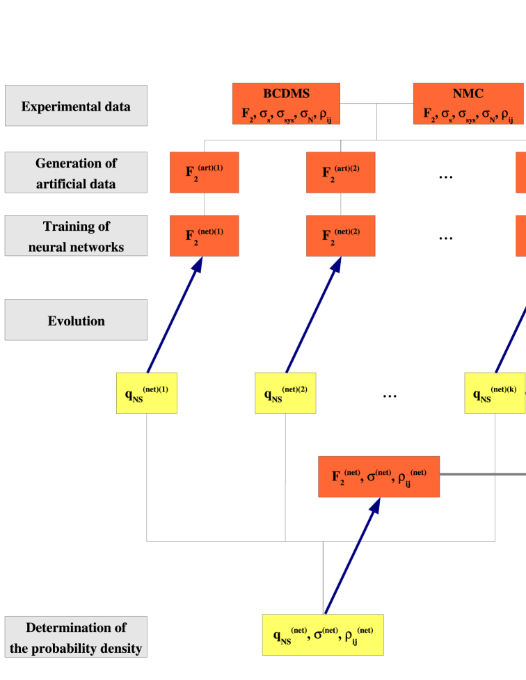
Figure 1: Flow-chart for the construction of a neural parton set.

The starting experimental data in general consist of the determination of several physical observables in distinct experiments, each of which provides the measurement of the relevant quantity at a discrete set of values of the kinematical variables. In general, there will be a nontrivial set of correlations between determination of different quantities: e.g., different observables determined at different points may be correlated both between observables and between points. In the current nonsinglet fit, we will consider a single observable, namely the nonsinglet nucleon structure function defined as

$$F_{2}^{\mathrm{NS}}(x,Q^{2})\equiv F_{2}^{p}(x,Q^{2})-F_{2}^{d}(x,Q^{2})\ ,$$ (1)

in terms of the proton and deuteron structure functions.

The purpose of the artificial data generation is to produce a Monte Carlo set of ‘pseudo–data’, i.e. $N_{\mathrm{rep}}$ replicas of the original set of $N_{\mathrm{dat}}$ data points:

$$F^{(\mathrm{art})(k)}_{i};\qquad k=1,\dots,N_{\mathrm{rep}},\quad i=1,\dots,N_{\mathrm{dat}},$$ (2)

where $F_{i}$ denotes one individual measurement: in our specific case, a measurement of $F^{\mathrm{NS}}_{2}(x_{i},Q^{2}_{i})$. The $N_{\mathrm{rep}}$ sets of $N_{\mathrm{dat}}$ points are distributed according to an $N_{\mathrm{dat}}$–dimensional multi-gaussian distribution about the original points, with expectation values equal to the central experimental values, and error and covariance equal to the corresponding experimental quantities. Because the distribution of the experimental data coincides (for a flat prior) with the probability distribution of the value of the structure function at the points where it has been measured [14, 15], this Monte Carlo set gives a sampling of the probability measure at those points. We can then generate arbitrarily many sets of pseudo–data, and choose the number of sets $N_{\mathrm{rep}}$ in such a way that the properties of the Monte Carlo sample reproduce those of the original data set to arbitrary accuracy. For example, we can check that averages, variance and covariance of the pseudo-data reproduce central values and covariance matrix elements of the original data. This step is denoted by ’Tests exp-art’ in Fig. 1. Note that experimental errors (including correlated systematics) must be treated as gaussian since this is what experimental collaborations provide: the relevant issue is whether an underlying non-gaussian distribution of best-fit parton distributions can be obtained as a result of the fitting procedure. Whereas this might be problematic if errors are determined as one–sigma contours for a given parametrization, the Monte Carlo method gives considerably more flexibility, as we now show.

The second step consists of training $N_{\mathrm{rep}}$ sets of neural networks. Each set contains all the parton distributions which are being determined, as a function of $x$ at a given reference scale $Q_{0}^{2}$, and is based on all the data in one single replica of the original data set. Thus, each set will contain $N_{\mathrm{pdf}}$ parton distributions, determined from $N_{\mathrm{dat}}$ data. The number of independent parton distributions is $1\leq N_{\mathrm{pdf}}\leq 13$, and it will depend on the specific data set which is used in the parton determination. At most, there can be six quark and antiquark distributions and one gluon distribution, but in practice not all of these may be accessible with a given set of data. Specifically, in the nonsinglet fit discussed in this paper we will consider the simplest possible case, in which each set contains only one parton distribution, namely the C-even nonsinglet quark distribution

$$q_{\mathrm{NS}}(x,Q_{0}^{2})\equiv\left[u(x,Q_{0}^{2})+\bar{u}(x,Q_{0}^{2})-(d(x,Q_{0}^{2})+\bar{d}(x,Q_{0}^{2}))\right].$$ (3)

As in any parton fit, in order to compare the parton distributions with the data, the PDFs must be evolved from the reference scale $Q_{0}^{2}$ to the scale at which data are given, and combined with hard partonic cross sections in order to obtain physical observables. Unlike in most parton fits (such as e.g. [6, 5, 4]), however, each parton distribution is parametrized by a neural network, rather than by a fixed functional form. Then, the $N_{\mathrm{dat}}$ data in each replica are used to determine the $N_{\mathrm{pdf}}$ neural networks of the corresponding set. At the end of the procedure, we end up with $N_{\mathrm{rep}}$ sets of $N_{\mathrm{pdf}}$ parton distributions, with each PDF given by a neural network. The $N_{\mathrm{rep}}$ replicas of each parton distribution provide the corresponding probability density: for example, the mean value of the parton distribution at the starting scale for a given value of $x$ is found by averaging over the replicas, and the uncertainty on this value is the variance of the values given by the replicas.

The fit of the parton distributions to each replica of the data is performed by maximum likelihood, by minimizing an error function, which coincides with the $\chi^{2}$ of the experimental points when compared to their theoretical determination obtained using the given set of parton distributions. The $\chi^{2}$ is computed by fully including the covariance matrix of the correlated experimental uncertainties (with a suitable treatment of normalization errors [14]), as we shall discuss in more detail in Sect. 5.1 below. Unlike in conventional determinations of parton distributions with errors [6, 5, 4], however, the covariance matrices of the best–fit parameters are irrelevant and need not be computed. The uncertainty on the final result is found from the variance of the Monte Carlo sample. This eliminates the problem of choosing the value of $\Delta\chi^{2}$ which corresponds to a one-sigma contour in the space of parameters, a problem which becomes nontrivial in the presence of incompatible data, underestimated errors, or unknown systematics, and which therefore plagues current global fits [6, 5].

Rather, one only has to make sure that each neural network provides a consistent fit to its corresponding replica. If the underlying data are incompatible or have underestimated errors, the best fit might be worse than one would expect with properly estimated gaussian errors — for instance in the presence of underestimated errors it will have typically a value of $\chi^{2}$ per degree of freedom larger than one. If, on the contrary, experimental errors have been overestimated, the final $\chi^{2}$ can turn out to be smaller than one per degree of freedom. Neural networks are ideally suited for providing a fit in this situation, based on the reasonable assumption of smoothness: for example, incompatible data or data with underestimated errors will naturally be fitted less accurately by the neural network [9]. Also, this allows for non-gaussian behavior of experimental uncertainties. Indeed, whereas a neural network with sufficiently large architecture can fit any compatible set of data, the choice of a suitable stopping criterion ensures that only the information contained in the data is fitted, but not the noise. This can be done by verifying that the quality of the fit of data which have been used in the fitting procedure is the same as the quality of the fit to data which have not been used for fitting.

It is then possible to verify that each neural network has the correct statistical features. This step is denoted by ’Tests net-art’ in Fig. 1. Finally, the self-consistency of the Monte Carlo sample can be tested in order to ascertain that it leads to consistent estimates of the uncertainty on the final parton distributions, for example by verifying that the value of the parton distribution extracted from different replicas indeed behaves as a random variable with the stated variance. This step is denoted by ’Tests net-net’ in Fig. 1. This set of tests allow us to make sure that the Monte Carlo sample of neural networks provides a faithful and consistent representation of the information contained in the data on the probability measure in the space of parton distributions, and in particular that the value of parton distributions and their correlated uncertainties are correctly estimated.

Because of the use of neural networks for the parametrization of the parton distributions, two technical aspects of our fitting procedure differ from what is done in standard parton fits. The first is the method which is used in order to evolve parton distributions by solving the QCD evolution equations. Indeed, we solve evolution equations in Mellin moment space $N$ [16], since this allows for a fast and accurate numerical solution. However, this method is usually applied to parton parametrizations such that the Mellin transform of the initial parton distribution can be computed analytically: a numerical approach is not viable because in the region where the inverse Mellin transform of the solution exists, the Mellin transform of the initial condition does not converge. But a neural network is a complicated nonlinear function whose Mellin transform cannot be determined analytically in closed form. The alternative of parametrizing directly the initial parton distributions in $N$ moment space is unpalatable, because one would need a parametrization in the complex plane of the $N$ variable, whereas neural networks are most conveniently defined on a compact space, such as $0\leq x\leq 1$.

Therefore, we are led to introduce a novel technique, which consists of determining the $x$–space evolution kernel (Green function) from the $N$ space solution, in such a way that any parton distribution can be evolved by convolution with this universal kernel. This method combines the speed and reliability of the $N$–space solution method, with the advantages of parametrizing the parton distribution in $x$ space. Furthermore, because the kernel is universal (i.e. independent of the specific boundary condition which is evolved) it can be computed beforehand to arbitrarily high accuracy and stored; the result can then be used during the fitting procedure, thus leading to an extremely efficient evolution. This evolution method will be discussed in detail in Sect. 4.

The other technical peculiarity which is motivated by the use of neural networks is the choice of the minimization algorithm. Because of the nonlinear dependence of the neural network on its parameters, and the nonlocal dependence of the measured quantities on the neural network (cross sections are expressed as convolution of the initial distribution with evolution kernels and coefficient functions), a genetic algorithm turns out to be the most efficient minimization method. The use of a genetic algorithm is particularly convenient when seeking a minimum in a very wide space with potentially many local minima, because the method handles a population of solutions rather than traversing a path in the space of solutions. The minimization method will be discussed in detail in Sect. 5.

At the end of the minimization we end up with a Monte Carlo sample of neural networks which provides our best representation of the measure in the space of parton distribution. Generally, we expect [9, 10] the uncertainty on our final result to be somewhat smaller than the uncertainty on the input data, because the information contained in several data points is combined. The properties of this measure can be tested against the input data by using it to compute means, variance and covariances which can be compared to the input experimental ones which have been used in the parton determination. Also, the stability of the result can be tested by excluding some data points from the fit and checking that the best-fit result predicts them correctly. These tests are denoted by ’Tests net-exp’ in Fig. 1, and they conclude our determination.

3 Experimental data and Monte Carlo generation

3.1 Experimental data and kinematical cuts

The nonsinglet parton distribution $q_{\mathrm{NS}}(x,Q_{0}^{2})$ can be extracted from experimental data on proton and deuteron structure functions $F_{2}^{p}(x,Q^{2})$ and $F_{2}^{d}(x,Q^{2})$. A detailed discussion of all the available data was given in Refs. [9, 10]. In short, early SLAC data have extremely large uncertainties, while data from JLAB and the E665 collaboration [17] are mostly at low $Q^{2}$ and are almost entirely excluded by our kinematic cuts. This leaves us with the data published by the NMC [18] and BCDMS [19, 20] collaborations. We refer to [9] for a discussion of the kinematical and statistical features of these data, in particular for the details of their correlated systematics.

Once the systematics are known, the experimental covariance matrix for each experiment can be easily computed

$${\rm cov}_{ij}=\left(\sum_{p=1}^{N_{\mathrm{sys}}}\sigma_{i,p}\sigma_{j,p}+F_{i}F_{j}\sigma_{N}^{2}\right)+\delta_{ij}\sigma_{i,s}^{2}\ ,$$ (4)

where $F_{i}$, $F_{j}$ are central values, $\sigma_{i,p}$ are the $N_{\mathrm{sys}}$ correlated systematic errors, $\sigma_{N}$ is the total normalization uncertainty, and $\sigma_{i,s}$ is the statistical uncertainty. The correlation matrix is given by

$$\rho_{ij}={{{\rm cov}_{ij}}\over{\sigma_{i,\mathrm{tot}}\sigma_{j,\mathrm{tot}}}}\ ,$$ (5)

where the total error $\sigma_{i,\mathrm{tot}}$ for the $i$-th point is given by

$$\sigma_{i,\mathrm{tot}}=\sqrt{\sigma_{i,s}^{2}+\sigma_{i,c}^{2}+F_{i}^{2}\sigma_{N}^{2}}\$$ (6)

and the total correlated uncertainty $\sigma_{i,c}$ is the sum of all correlated systematics

$$\sigma_{i,c}^{2}=\sum_{p=1}^{N_{\mathrm{sys}}}\sigma_{i,p}^{2}\ .$$ (7)

In order to keep higher twist corrections under control, only data with $Q^{2}>$ 3 GeV² are retained. No separate cut in the invariant mass of the final state $W^{2}$ turns out to be necessary. A discussion on the motivation for this choice of cuts and the possible effect of their variation will be given in Sect. 6.

A scatter plot of the NMC and BCDMS data in the $(x,Q^{2})$ plane is displayed in Fig. 2, with points excluded due to the $Q^{2}$ cut marked with diamonds. Note that all these excluded data points belong to the NMC experiment. In Table 1, the statistical features of the data (after the cut) are summarized.

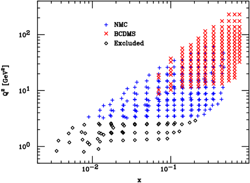
Figure 2: Kinematical coverage of the available experimental data on the nonsinglet structure function in the $(x,Q^{2})$ plane.

Experiment	$x$ range	$Q^{2}$ range	$N_{\mathrm{dat}}$	$\left\langle\sigma_{s}\right\rangle$	$\left\langle\sigma_{c}\right\rangle$	$\left\langle{{\sigma_{c}}\over{\sigma_{s}}}\right\rangle$	$\left\langle\sigma_{N}\right\rangle$	$\left\langle\sigma_{\mathrm{tot}}\right\rangle$	$\left\langle\rho\right\rangle$	$\left\langle\mathrm{cov}\right\rangle$
NMC	$9.0~{}10^{-3}~{}-~{}4.7~{}10^{-1}$	$3.2-61$ GeV2	229	103.2	85.6	0.75	72.5	157.5	0.038	0.199
BCDMS	$7.0~{}10^{-2}~{}-~{}7.5~{}10^{-1}$	$8.7-230$ GeV2	254	22.3	12.2	0.50	22.3	37.3	0.163	0.085

Table 1: Experimental data included in this analysis. All values of $\sigma$ and cov are given as percentages. Averages over all data points are noted with brackets $\langle\rangle$.

$F_{2}^{\mathrm{NS}}(x,Q^{2})$
$N_{\mathrm{rep}}$	10	100	1000
$\left\langle PE\left[\left\langle F^{(\mathrm{art})}\right\rangle_{\mathrm{rep}}\right]\right\rangle$	20%	6.4%	1.3%
$r\left[F^{(\mathrm{art})}\right]$	0.97	0.99	0.99
$\left\langle V\left[\sigma^{(\mathrm{art})}\right]\right\rangle_{\mathrm{dat}}$	$6.1~{}10^{-5}$	$1.9~{}10^{-5}$	$6.7~{}10^{-6}$
$\left\langle PE\left[\sigma^{(\mathrm{art})}\right]\right\rangle_{\mathrm{dat}}$	33%	11%	3%
$\left\langle\sigma^{(\mathrm{art})}\right\rangle_{\mathrm{dat}}$	0.011	0.011	0.011
$r\left[\sigma^{(\mathrm{art})}\right]$	0.94	0.99	0.99
$\left\langle V\left[\rho^{(\mathrm{art})}\right]\right\rangle_{\mathrm{dat}}$	$0.10$	$9.4~{}10^{-3}$	$1.0~{}10^{-3}$
$\left\langle\rho^{(\mathrm{art})}\right\rangle_{\mathrm{dat}}$	0.182	0.097	0.100
$r\left[\rho^{(\mathrm{art})}\right]$	0.47	0.79	0.97
$\left\langle V\left[\mathrm{cov}^{(\mathrm{art})}\right]\right\rangle_{\mathrm{dat}}$	$5.5~{}10^{-9}$	$1.7~{}10^{-10}$	$5.7~{}10^{-11}$
$\left\langle\mathrm{cov}^{(\mathrm{art})}\right\rangle_{\mathrm{dat}}$	$1.3~{}10^{-5}$	$7.6~{}10^{-6}$	$8.1~{}10^{-6}$
$r\left[\mathrm{cov}^{(\mathrm{art})}\right]$	0.41	0.81	0.98

Table 2: Comparison between experimental and Monte Carlo data. The experimental data have $\left\langle\sigma^{(\mathrm{exp})}\right\rangle_{\mathrm{dat}}=0.011$, $\left\langle\rho^{(\mathrm{exp})}\right\rangle_{\mathrm{dat}}=0.107$ and $\left\langle\mathrm{cov}^{(\mathrm{exp})}\right\rangle_{\mathrm{dat}}=8.6~{}10^{-6}$.

3.2 Monte Carlo generation

The first step in our approach, as discussed in Sect. 2, is to generate a Monte Carlo sample of replicas of the experimental data. Each Monte Carlo replica of the original experimental data is generated as a multi-gaussian distribution. More precisely, for each data point $F_{i}^{\rm(exp)}\equiv F_{2}^{\mathrm{NS}}(x_{i},Q^{2}_{i})$ we generate $k=1,\ldots,N_{\mathrm{rep}}$ artificial points $F^{(\mathrm{art})(k)}$ as follows

$$F_{i}^{(\mathrm{art})(k)}=\left(1+r_{N}^{(k)}\sigma_{N}\right)\left(F_{i}^{\rm(\mathrm{exp})}+\sum_{p=1}^{N_{\mathrm{sys}}}r_{p}^{(k)}\sigma_{i,p}+r_{i}^{(k)}\sigma_{i,s}\right)\ ,\ k=1,\ldots,N_{\mathrm{rep}}\ ,$$ (8)

using independent univariate gaussian random numbers $r^{(k)}$ for each independent error source.

The value of $N_{\mathrm{rep}}$ is determined in such a way that the Monte Carlo set of replicas models faithfully the probability distribution of the data in the original set. A quantitative comparison can be performed by defining suitable statistical estimators (see Appendix B). Results are presented in Table 2. The results show that a sample of 1000 replicas is sufficient to ensure average scatter correlations of 99% and accuracies of a few percent on structure functions, errors and correlations.

Normalization errors are not included in the covariance matrix on the same footing as other sources of systematics since, as by now well known [14], this would bias the fit. Rather, normalization errors are included by rescaling all errors (statistical $\sigma_{i,s}$ and each systematic $\sigma_{i,p}$) independently for each replica by a factor

$$\overline{\sigma}_{i,s}^{(k)} = (1+r^{(k)}_{N}\sigma_{N})\sigma_{i,s}\ ,$$

$$\overline{\sigma}_{i,p}^{(k)} = (1+r^{(k)}_{N}\sigma_{N})\sigma_{i,p}\qquad p=1\ ,\ldots,N_{\mathrm{sys}}\ ,$$ (9)

where $r^{(k)}_{N}$ is the random variable Eq. (8) associated to the normalization uncertainty. The covariance matrix is then given by

$${\overline{\mathrm{cov}}^{(k)}}_{ij}=\left(\sum_{p=1}^{N_{\mathrm{sys}}}{\overline{\sigma}^{(k)}}_{i,p}{\overline{\sigma}^{(k)}}_{j,p}\right)+\delta_{ij}{\overline{\sigma}^{(k)2}}_{i,s}\ ,$$ (10)

in terms of the rescaled uncertainties.

4 From parton distributions to physical observables

The nonsinglet structure function $F_{2}^{\mathrm{NS}}(x,Q^{2})$ Eq. (1) is determined from the nonsinglet quark distribution $q_{\mathrm{NS}}(x,Q_{0}^{2})$ Eq. (3) at a reference scale $Q_{0}^{2}$ by first evolving the parton distribution to the scale $Q^{2}$ by means of QCD evolution equations, and then convoluting it with the appropriate hard coefficient function $C_{\mathrm{NS}}(x,\alpha_{s}\left(Q^{2}\right))$:

$$F_{2}^{\mathrm{NS}}(x,Q^{2})={{1}\over{6}}x\int_{x}^{1}{{dy}\over{y}}C_{\mathrm{NS}}(y,\alpha_{s}\left(Q^{2}\right))q_{\mathrm{NS}}\left({{x}\over{y}},Q^{2}\right)\ .$$ (11)

Both coefficient functions and the anomalous dimensions which drive perturbative evolution are now known up to next-to-next-to leading order (and in fact the coefficient function up to NNNLO [21]). Therefore, we will provide determinations of the parton distributions at leading (LO), next-to-leading (NLO) and next-to-next-to leading order (NNLO). In this section we will discuss in detail the methods that we use in order to actually determine the structure function from the input parton distribution, specifically the resolution of evolution equations. Only the nonsinglet case will be discussed explicitly, while the (straightforward) generalization to the singlet case will be discussed in a forthcoming publication.

4.1 Leading-twist evolution and coefficient functions

As well known, QCD evolution equations are most easily written for Mellin moments of the parton distributions, defined as

$$q_{\mathrm{NS}}(N,Q^{2})\equiv\int_{0}^{1}\!dx\,x^{N-1}q_{\mathrm{NS}}(x,Q^{2})\ ,$$ (12)

where by slight abuse of notation we denote the function and its transform with the same symbol. They take the form

$${{d}\over{d\ln Q^{2}}}q_{\mathrm{NS}}(N,Q^{2})={{\alpha_{s}\left(Q^{2}\right)}\over{4\pi}}\gamma_{\mathrm{NS}}(N,\alpha_{s}\left(Q^{2}\right))\,q_{\mathrm{NS}}(N,Q^{2})\ ,$$ (13)

where the anomalous dimension can be expanded in powers of $\alpha_{s}\left(Q^{2}\right)$ as

$$\gamma_{\mathrm{NS}}(N,\alpha_{s}\left(Q^{2}\right))=\gamma^{(0)}_{\mathrm{NS}}(N)+{{\alpha_{s}\left(Q^{2}\right)}\over{4\pi}}\gamma^{(1)}_{\mathrm{NS}}(N)+\left({{\alpha_{s}\left(Q^{2}\right)}\over{4\pi}}\right)^{2}\gamma^{(2)}_{\mathrm{NS}}(N)+\dots$$ (14)

The NNLO contribution has been computed recently in Ref. [22]. Defining analogously the Mellin transforms of coefficient function and structure function, the latter is given by

$$F_{2}^{\mathrm{NS}}(N-1,Q^{2})={{1}\over{6}}C_{\mathrm{NS}}(N,\alpha_{s}\left(Q^{2}\right))q_{\mathrm{NS}}\left(N,Q^{2}\right),$$ (15)

with the perturbative expansion of the coefficient function

$$C_{\mathrm{NS}}(N,\alpha_{s}\left(Q^{2}\right))=1+{{\alpha_{s}\left(Q^{2}\right)}\over{4\pi}}C_{\mathrm{NS}}^{(1)}(N)+\left({{\alpha_{s}\left(Q^{2}\right)}\over{4\pi}}\right)^{2}C_{\mathrm{NS}}^{(2)}(N)+\dots.$$ (16)

It appears therefore especially convenient [16, 23] to determine the structure function in Mellin space and then invert the Mellin transform, since the $N$ space expression of the structure function can be determined in closed form, and the problem is reduced to the computation of the single Mellin inversion integral. In $x$-space instead one has to solve an integro–differential equation. Even though efficient numerical methods have been developed for the resolution of the integro-differential form of the evolution equation (see e.g. [24, 25]), the only genuine advantage of an $x$–space approach is the possibility to work directly with an $x$–space parametrization of parton distributions. As discussed in Sect. 2, this option is especially convenient when using neural networks, since these are most easily defined as function on a compact space such as $0\leq x\leq 1$.

However, we observe that the solution to the evolution equation (13) has the form

$$q_{\mathrm{NS}}(N,Q^{2})=\Gamma(N,\alpha_{s}\left(Q^{2}\right),\alpha_{s}\left(Q^{2}_{0}\right))q_{\mathrm{NS}}(N,Q^{2}_{0})\ ,$$ (17)

where the evolution kernel $\Gamma(N,\alpha_{s}\left(Q^{2}\right),\alpha_{s}\left(Q^{2}_{0}\right))$ is entirely determined by the anomalous dimension $\gamma_{\mathrm{NS}}(N,\alpha_{s}\left(Q^{2}\right))$, and it does not depend on the boundary condition $q_{\mathrm{NS}}(N,Q^{2}_{0})$. Hence, if we take an inverse Mellin transform of Eq. (17) we get

$$q_{\mathrm{NS}}(x,Q^{2})=\int_{x}^{1}{{dy}\over{y}}\Gamma(y,\alpha_{s}\left(Q^{2}\right),\alpha_{s}\left(Q^{2}_{0}\right))q_{\mathrm{NS}}\left({{x}\over{y}},Q_{0}^{2}\right).$$ (18)

We can then determine the kernel $\Gamma(x,\alpha_{s}\left(Q^{2}\right),\alpha_{s}\left(Q^{2}_{0}\right))$ explicitly by Mellin inversion, and use it to evolve any $x$–space parton distribution using Eq. (18). The only complication is related to the large-$x$ behavior of the kernel $\Gamma(x,\alpha_{s}\left(Q^{2}\right),\alpha_{s}\left(Q^{2}_{0}\right))$.

Furthermore, we can express the structure function in terms of the initial quark distribution as

$$F_{2}^{\mathrm{NS}}(N-1,Q^{2})={{1}\over{6}}\widetilde{\Gamma}(N,\alpha_{s}\left(Q^{2}\right),\alpha_{s}\left(Q^{2}_{0}\right))\,q_{\mathrm{NS}}(N,Q^{2}_{0})\ ,$$ (19)

where

$$\widetilde{\Gamma}(N,\alpha_{s}\left(Q^{2}\right),\alpha_{s}\left(Q^{2}_{0}\right))\equiv C_{\mathrm{NS}}(N,\alpha_{s}\left(Q^{2}\right))\Gamma(N,\alpha_{s}\left(Q^{2}\right),\alpha_{s}\left(Q^{2}_{0}\right)),$$ (20)

i.e. absorbing the coefficient function in a redefined evolution kernel. Again, we can determine the Mellin inverse of this redefined kernel, and use it to obtain the measured structure function from the initial $x$–space parton distribution as

$$F_{2}^{\mathrm{NS}}(x,Q^{2})={{1}\over{6}}x\int_{x}^{1}{{dy}\over{y}}\tilde{\Gamma}(y,\alpha_{s}\left(Q^{2}\right),\alpha_{s}\left(Q^{2}_{0}\right))\,q_{\mathrm{NS}}\left({{x}\over{y}},Q_{0}^{2}\right)\ .$$ (21)

The evolution kernels can be computed, interpolated to arbitrary accuracy and stored, and then used to evolve the initial PDF or determine the structure function from it through the computation of a single real convolution integral, eqs. (18) and (21).

4.2 Solution of the evolution equation in $N$ space

We determine the evolution kernel up to NNLO in terms of the running coupling, for which we take the expanded solution of the renormalization group equation, i.e., up to NNLO

$$\alpha_{s}\left(Q^{2}\right) = \alpha_{s}\left(Q^{2}\right)_{LO}\Bigg{[}1+\alpha_{s}\left(Q^{2}\right)_{LO}\left[\alpha_{s}\left(Q^{2}\right)_{LO}-\alpha_{s}\left(M_{Z}^{2}\right)\right](b_{2}-b_{1}^{2})$$ (22)

$$+ \alpha_{s}\left(Q^{2}\right)_{NLO}b_{1}\ln{{\alpha_{s}\left(Q^{2}\right)_{NLO}}\over{\alpha_{s}\left(M_{Z}^{2}\right)}}\Bigg{]},$$

with

$$\alpha_{s}\left(Q^{2}\right)_{NLO}=\alpha_{s}\left(Q^{2}\right)_{LO}\left[1-b_{1}\alpha_{s}\left(Q^{2}\right)_{LO}\ln\left(1+\beta_{0}\alpha_{s}\left(M_{Z}^{2}\right)\ln{{Q^{2}}\over{M_{Z}^{2}}}\right)\right]\ ,$$ (23)

$$\alpha_{s}\left(Q^{2}\right)_{LO}={{\alpha_{s}\left(M_{Z}^{2}\right)}\over{1+\beta_{0}\alpha_{s}\left(M_{Z}^{2}\right)\ln{{Q^{2}}\over{M_{Z}^{2}}}}},$$ (24)

and the beta function coefficients given by

$$Q^{2}{{da_{s}(Q^{2})}\over{dQ^{2}}}=-\sum_{k=0}^{2}\beta_{k}a_{s}(Q^{2})^{k+2},\qquad a_{s}(Q^{2})={{\alpha_{s}(Q^{2})}\over{4\pi}}\,,$$ (25)

where

$$\beta_{0} = 11-{{2}\over{3}}N_{f}\ ,$$ (26)

$$\beta_{1} = 102-{{38}\over{3}}N_{f}\ ,$$ (27)

$$\beta_{2} = {{2857}\over{2}}-{{5033}\over{18}}N_{f}+{{325}\over{54}}N_{f}^{2}\ ,$$ (28)

and $b_{i}\equiv\beta_{i}/\beta_{0}$. We will use the current PDG [26] average value of $\alpha_{s}\left(Q^{2}\right)$, namely

$$\alpha_{s}(M_{Z}^{2})=0.118\pm 0.002$$ (29)

with $M_{Z}=91.187$ GeV.

The evolution factor is then explicitly given by

$$\Gamma(N,\alpha_{s}\left(Q^{2}\right),\alpha_{s}\left(Q^{2}_{0}\right))=\left({{\alpha_{s}\left(Q^{2}\right)}\over{\alpha_{s}\left(Q^{2}_{0}\right)}}\right)^{-\gamma^{(0)}(N)/\beta_{0}}\Bigg{(}1-\left(a_{s}(Q^{2})-a_{s}(Q^{2}_{0})\right)U_{\mathrm{NS}}^{(1)}(N)$$

$$\qquad+\left(a^{2}_{s}(Q^{2})-a^{2}_{s}(Q^{2}_{0})\right)U_{\mathrm{NS}}^{(2)}(N)-a_{s}(Q^{2})a_{s}(Q_{0}^{2})\left(U_{\mathrm{NS}}^{(1)}(N)\right)^{2}\Bigg{)}\ ,$$ (30)

where (adopting the notations and conventions of Ref. [23]) we have introduced nonsinglet evolution coefficients

$$U_{\mathrm{NS}}^{(1)}(N)=-{{1}\over{\beta_{0}}}\left(\gamma^{(1)}(N)-b_{1}\gamma^{(0)}(N)\right)\ ,$$ (31)

$$U_{\mathrm{NS}}^{(2)}(N)=-{{1}\over{2}}\left[{{1}\over{\beta_{0}}}\gamma^{(2)}(N)-b_{1}U_{\mathrm{NS}}^{(1)}-{{b_{2}}\over{\beta_{0}}}\gamma^{(0)}(N)-\left(U_{\mathrm{NS}}^{(1)}(N)\right)^{2}\right]\,.$$ (32)

At NNLO, both the strong coupling and the parton distributions are discontinuous when crossing heavy quark thresholds. We set the thresholds $m_{c}=1.4~{}{\rm GeV}$, $m_{b}=4.5~{}{\rm GeV}$ and $m_{t}=175~{}{\rm GeV}$ with, at NNLO, the discontinuity

$$\alpha_{s,f+1}(m_{f}^{2})=\alpha_{s,f}(m_{f}^{2})+\left({{C_{2}}\over{4\pi}}\right)^{2}\alpha_{s,f}(m_{f}^{2})^{3}\ ,$$ (33)

where $C_{2}=14/3$ [27]. We match parton distributions at threshold as

$$q_{\mathrm{NS}}^{(n_{f}+1)}(N,m_{h}^{2})=q_{\mathrm{NS}}^{(n_{f})}(N,m_{h}^{2})\ .$$ (34)

Heavy quark mass terms are included in the hard coefficients, and in the nonsinglet sector they vanish up to NLO, while at NNLO they are not known (though they can be approximated from their large $x$ behavior [28]). Therefore, we defer the inclusion of heavy quark mass effects to a forthcoming full fit including the singlet contribution, hence, for all practical purposes, we use a zero–mass variable flavour number scheme in the nonsinglet sector. Note that because of this, the nonsinglet structure function $F_{2}^{\mathrm{NS}}$ has a NNLO discontinuity at the heavy quark thresholds.

4.3 Evolution kernel in $x$-space

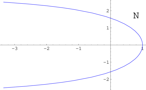
Figure 3: The path in the complex N-space followed by the Talbot integration path, Eq. (36) for $r=1$.

The $x$–space evolution factor is determined by numerical computation of the Mellin inverse

$$\Gamma(x,\alpha_{s}\left(Q^{2}\right),\alpha_{s}\left(Q^{2}_{0}\right))=\int_{c-i\infty}^{c+i\infty}{{dN}\over{2\pi i}}x^{-N}\Gamma(N,\alpha_{s}\left(Q^{2}\right),\alpha_{s}\left(Q^{2}_{0}\right))\ ,$$ (35)

of the $N$ space evolution factor $\Gamma(N,\alpha_{s}\left(Q^{2}\right),\alpha_{s}\left(Q^{2}_{0}\right))$, Eq. (4.2), as well as of the associate $\tilde{\Gamma}(N,\alpha_{s}\left(Q^{2}\right),\alpha_{s}\left(Q^{2}_{0}\right))$, Eq. (20). The numerical computation of the Mellin inversion integral is delicate, because the oscillatory behavior of the integrand at large $x$ is not damped by multiplication by an initial PDF. This problem is mitigated by a suitable choice of integration path. We choose the Talbot path, defined by the condition

$$N(\theta)=r\theta\left(1/\tan\theta+i\right),\quad-\pi\leq\theta\leq\pi\ ,$$ (36)

with $r$ a constant, shown in Fig. 3.

To further improve the numerical efficiency the Fixed Talbot algorithm can be used [29] where the integral is replaced by the sum

$$\Gamma\left(x\right)={{r}\over{M}}\left[{{1}\over{2}}\Gamma\left(N=r\right)x^{-r}+\sum_{k=1}^{M-1}\mathrm{Re}\left[x^{-N\left(\theta_{k}\right)}\Gamma\left(N\left(\theta_{k}\right)\right)\left(1+i\sigma\left(\theta_{k}\right)\right)\right]\right]$$ (37)

where $\sigma\left(\theta\right)\equiv\theta+\left(\theta/\tan\theta-1\right)/\tan\theta$, and $\theta_{k}=k\pi/M$, and $r=2M/\left(5\ln 1/x\right)$. It can be shown that $M$ is the relative accuracy, i.e. the number of accurate digits. We shall take $M=16$. The $x-$space evolution kernel $\Gamma(x)$ determined thus is displayed in Fig. 5, at different perturbative orders and in Fig. 5 for different values of $Q^{2}$.

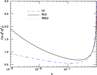
Figure 4: Non-singlet evolution kernel $\Gamma(x)$ computed at different perturbative orders in the kinematical region relevant to nonsinglet evolution. The evolution scales are $Q_{0}^{2}=2$ GeV² and $Q^{2}=10^{4}$ GeV².

Figure 5: Same as Fig. 5 for the LO dependence of the evolution factor on the evolution length $Q^{2}$. As in the previous case, $Q_{0}^{2}=2$ GeV².

The determination of the evolution kernel presented so far only holds for $x<1$. As well known (see Appendix A), the Mellin inverse of the anomalous dimension Eq. (14) only exists for $x<1$, while at $x=1$ it behaves as a distribution. Because the $N$–space evolution kernel is obtained by exponentiating the anomalous dimension, its Mellin transform must be defined through its action on a test function. In particular, we must check that integration over the kernel converges as $x\to 1$. To this purpose, we define a subtracted kernel $\Gamma^{(+)}(x,\alpha_{s}\left(Q^{2}\right),\alpha_{s}\left(Q^{2}_{0}\right))$

$$\Gamma(x,\alpha_{s}\left(Q^{2}\right),\alpha_{s}\left(Q^{2}_{0}\right)) = \Gamma^{(+)}(x,\alpha_{s}\left(Q^{2}\right),\alpha_{s}\left(Q^{2}_{0}\right))+G\delta(1-x)\ ,$$ (38)

$$\Gamma^{(+)}(x,\alpha_{s}\left(Q^{2}\right),\alpha_{s}\left(Q^{2}_{0}\right)) \equiv \Gamma(x,\alpha_{s}\left(Q^{2}\right),\alpha_{s}\left(Q^{2}_{0}\right))-G\delta(1-x).$$ (39)

The constant $G$ is defined as

$$G\equiv\int_{0}^{1}dx\Gamma(x,\alpha_{s}\left(Q^{2}\right),\alpha_{s}\left(Q^{2}_{0}\right))=\Gamma(N,\alpha_{s}\left(Q^{2}\right),\alpha_{s}\left(Q^{2}_{0}\right))\Big{|}_{N=1}\ ,$$ (40)

where $\Gamma(N,\alpha_{s}\left(Q^{2}\right),\alpha_{s}\left(Q^{2}_{0}\right))$ is given by Eq. (4.2), and it converges at $N=1$.

The evolution equation, Eq.( 18), in terms of the subtracted kernel takes the form

$$q(x,Q^{2}) = Gq(x,Q_{0}^{2})+\int_{x}^{1}{{dy}\over{y}}\Gamma^{(+)}(y,\alpha_{s}\left(Q^{2}\right),\alpha_{s}\left(Q^{2}_{0}\right))q\left({{x}\over{y}},Q_{0}^{2}\right)$$ (41)

$$= q(x,Q_{0}^{2})\left(G-\int_{0}^{x}dy\Gamma(y,\alpha_{s}\left(Q^{2}\right),\alpha_{s}\left(Q^{2}_{0}\right))\right)$$

$$+ \int_{x}^{1}{{dy}\over{y}}\Gamma(y,\alpha_{s}\left(Q^{2}\right),\alpha_{s}\left(Q^{2}_{0}\right))\left(q\left({{x}\over{y}},Q_{0}^{2}\right)-yq(x,Q_{0}^{2})\right).$$

It is easy to prove that all integrals in Eq. (41) converge and can be computed numerically, exploiting the fact that the behavior of the evolution kernel in the large $x$ limit is known from soft gluon resummation arguments. An explicit proof is given in Appendix A.

Hence we will use Eq. (41) to determine the evolution of the quark distribution. The numerical accuracy of this method is tested by comparing it to the benchmark evolution tables first presented in Ref. [30] and recently updated including the full NNLO anomalous dimension in Ref. [2]. In order to allow for a direct comparison to the benchmark tables, we modify some of our final choices in the solution of the evolution equations. Specifically, we fix the number of flavors (to $n_{f}=4$) and we keep the NLO contributions to the evolution factor Eq. (4.2) in unexpanded form. With these choices, we determine the evolution of the $u$ valence parton distribution. The results and the accuracy of this benchmark are shown in Table 3, where we use the same parameters as in [30, 2]. More details about the benchmarking of QCD evolution codes can be found in Ref. [2]. We find an accuracy of order $\mathcal{O}\left(10^{-5}\right)$, comparable to that of current evolution codes. The same result has been obtained for the $d$ valence distribution. Comparable accuracy is expected in $C$–even evolution, relevant for our paper (not included in the benchmark [30])

x	$xu_{v}(x,Q^{2}_{0})$ (LH)	$xu_{v}(x,Q^{2}_{0})$ (NNPDF)	Rel. error
Leading order
$10^{-7}$	$5.7722~{}10^{-5}$	$5.7722~{}10^{-5}$	$3.3760~{}10^{-6}$
$10^{-6}$	$3.3373~{}10^{-4}$	$3.3373~{}10^{-4}$	$1.6880~{}10^{-6}$
$10^{-5}$	$1.8724~{}10^{-3}$	$1.8724~{}10^{-3}$	$1.9212~{}10^{-6}$
$10^{-4}$	$1.0057~{}10^{-2}$	$1.0057~{}10^{-2}$	$1.4095~{}10^{-6}$
$10^{-3}$	$5.0392~{}10^{-2}$	$5.0392~{}10^{-2}$	$2.6145~{}10^{-6}$
$10^{-2}$	$2.1955~{}10^{-1}$	$2.1955~{}10^{-1}$	$3.1065~{}10^{-6}$
$0.1$	$5.7267~{}10^{-1}$	$5.7267~{}10^{-1}$	$6.4524~{}10^{-6}$
$0.3$	$3.7925~{}10^{-1}$	$3.7925~{}10^{-1}$	$9.2674~{}10^{-6}$
$0.5$	$1.3476~{}10^{-1}$	$1.3476~{}10^{-1}$	$1.1307~{}10^{-5}$
$0.7$	$2.3123~{}10^{-2}$	$2.3122~{}10^{-2}$	$2.1165~{}10^{-5}$
$0.9$	$4.3443~{}10^{-4}$	$4.3440~{}10^{-4}$	$6.3630~{}10^{-5}$
Next-to-Leading order
$10^{-7}$	$1.0616~{}10^{-4}$	$1.0616~{}10^{-4}$	$2.1462~{}10^{-6}$
$10^{-6}$	$5.4177~{}10^{-4}$	$5.4177~{}10^{-4}$	$8.7799~{}10^{-6}$
$10^{-5}$	$2.6870~{}10^{-3}$	$2.6870~{}10^{-3}$	$9.7796~{}10^{-6}$
$10^{-4}$	$1.2841~{}10^{-2}$	$1.2841~{}10^{-2}$	$1.3380~{}10^{-5}$
$10^{-3}$	$5.7926~{}10^{-2}$	$5.7926~{}10^{-2}$	$8.5063~{}10^{-6}$
$10^{-2}$	$2.3026~{}10^{-1}$	$2.3026~{}10^{-1}$	$3.0757~{}10^{-7}$
$0.1$	$5.5452~{}10^{-1}$	$5.5452~{}10^{-1}$	$7.6419~{}10^{-7}$
$0.3$	$3.5393~{}10^{-1}$	$3.5393~{}10^{-1}$	$2.6979~{}10^{-6}$
$0.5$	$1.2271~{}10^{-1}$	$1.2271~{}10^{-1}$	$2.4466~{}10^{-5}$
$0.7$	$2.0429~{}10^{-2}$	$2.0429~{}10^{-2}$	$1.4810~{}10^{-5}$
$0.9$	$3.6096~{}10^{-4}$	$3.6094~{}10^{-4}$	$6.0762~{}10^{-5}$
Next-to-Next-to-Leading order
$10^{-7}$	$1.5287~{}10^{-4}$	$1.5287~{}10^{-4}$	$1.5497~{}10^{-5}$
$10^{-6}$	$6.9176~{}10^{-4}$	$6.9176~{}10^{-4}$	$5.0711~{}10^{-6}$
$10^{-5}$	$3.0981~{}10^{-3}$	$3.0981~{}10^{-3}$	$9.5455~{}10^{-6}$
$10^{-4}$	$1.3722~{}10^{-2}$	$1.3722~{}10^{-2}$	$1.8022~{}10^{-5}$
$10^{-3}$	$5.9160~{}10^{-2}$	$5.9160~{}10^{-2}$	$5.0631~{}10^{-6}$
$10^{-2}$	$2.3078~{}10^{-1}$	$2.3078~{}10^{-1}$	$2.4853~{}10^{-6}$
$0.1$	$5.5177~{}10^{-1}$	$5.5177~{}10^{-1}$	$2.4747~{}10^{-6}$
$0.3$	$3.5071~{}10^{-1}$	$3.5071~{}10^{-1}$	$2.8430~{}10^{-7}$
$0.5$	$1.2117~{}10^{-1}$	$1.2117~{}10^{-1}$	$3.5893~{}10^{-5}$
$0.7$	$2.0077~{}10^{-2}$	$2.0077~{}10^{-2}$	$5.5823~{}10^{-6}$
$0.9$	$3.5111~{}10^{-4}$	$3.5109~{}10^{-4}$	$5.8172~{}10^{-5}$

Table 3: Comparison of the Les Houches parton evolution benchmark results (LH) with our results (NNPDF).

The solution of the evolution equation through the determination of an evolution factor is particularly efficient because of the universality of the evolution factor itself, i.e., its independence of the specific boundary condition which is being evolved. Hence, the evolution factor can be precomputed and stored, and then used during the process of parton fitting or when evolving different parton distributions, without having to recompute it each time.

This fact can be exploited in an optimal way during parton fitting and parton evolution. In parton fitting, a given boundary condition must be evolved many times up to the fixed pairs of values of $(x,Q^{2})$ at which data are available (in our case, those shown in Fig. 2). Namely, for the $i$-th data point, one must compute $q(x_{i},Q^{2}_{i})$ given by Eq. (41). The constant $G$ Eq. (40) (which depends only on $Q^{2}_{i}$) can be precomputed and stored for all required values of $Q^{2}$. Furthermore, the numerical determination of the integral over $y$ on the right–hand side of Eq. (41) involves the determination of the integrand at a set of values of $y=y_{ki}$, which in turn depend on the given values of $x_{i},Q^{2}_{i}$: $y_{ki}=y_{ki}(x_{i},Q^{2}_{i})$. The integrand is fully determined by knowledge of the following values of initial parton distribution and of the evolution kernel:

$$\Gamma_{ik} \equiv \Gamma(y_{ik},\alpha_{s}(Q_{i}^{2}),\alpha_{s}\left(Q^{2}_{0}\right))$$ (42)

$$\tilde{q}_{ik} \equiv q\left({{x_{i}}\over{y_{ik}}},Q_{0}^{2}\right)-y_{ik}q(x_{i},Q_{0}^{2}).$$ (43)

The most computing–intensive task is the determination of the values $\Gamma_{ik}$ Eq. (42) of evolution kernel. We have precomputed and stored these values for all the necessary values of $x_{i}$, $Q^{2}_{i}$ and $y_{ik}$. In practice, we use gaussian integration with $N_{\rm pt}=16\left(2^{N_{\rm it}+1}-1\right)$ points and determine the values of $y$ accordingly. In Table 4 we show the percentage deviation $\epsilon$ of the left-hand side of Eq. (41), when compared to what is obtained from the use of a library routine with nominal percentage accuracy of $10^{-5}$. It is apparent that $N_{\rm it}=4$, i.e. integration with about 500 points is sufficient to reach this accuracy.

$N_{\rm it}$	$\left\langle\epsilon\right\rangle$	$\sigma_{\epsilon}$	$\epsilon_{\rm max}$	# of points with $\epsilon\geq 5~{}10^{-5}$.
1	$2.4~{}10^{-2}$	$8.5~{}10^{-2}$	$6.6~{}10^{-1}$	21.3%
2	$1.3~{}10^{-4}$	$6.2~{}10^{-4}$	$4.0~{}10^{-3}$	7.2%
4	$1.6~{}10^{-5}$	$1.5~{}10^{-4}$	$3.3~{}10^{-3}$	5.4%
6	$1.6~{}10^{-5}$	$1.5~{}10^{-4}$	$3.3~{}10^{-3}$	5.4%

Table 4: Relative accuracy $\epsilon$ (see text) in the result obtained for NLO evolution as a function of the number of points $N_{\rm pt}=16\left(2^{N_{\rm it}+1}-1\right)$ used for gaussian integration.

This method is of course only convenient when evolving up to a fixed set of points in the $(x,Q^{2})$ plane. When evolving up a parton distribution, e.g. in order to input it to some other computation, it is instead convenient to precompute a full interpolation of the kernel $\Gamma(x,\alpha_{s}\left(Q^{2}\right),\alpha_{s}\left(Q^{2}_{0}\right))$. Evolution is then reduced to the determination of the convolution Eq. (41) of this kernel with the parton distribution. This is somewhat less efficient than the previous method because it requires the computation of this convolution over the interpolation each time a point is evolved, but it already avoids the main bottleneck, namely, the Mellin inversion of the kernel. We have interpolated the kernel $\Gamma(x,\alpha_{s}\left(Q^{2}\right),\alpha_{s}\left(Q^{2}_{0}\right))$ and its integral up to $x$ which appears in the first term of Eq. (41), using Chebyshev polynomials.

In order to speed up the interpolation, the leading large $x$ behavior determined at each perturbative order (as described in Appendix A) is divided out before interpolating, which considerably smoothes the large $x$ growth of $\Gamma(x,\alpha_{s}\left(Q^{2}\right),\alpha_{s}\left(Q^{2}_{0}\right))$. We have found that the use of 200 polynomials for the interpolation considered above produces results with a precision of $\mathcal{O}\left(10^{-5}\right)$, for all the $(x,Q^{2})$ range covered by experimental data. This accuracy is enough for present purposes and it could be improved by increasing the number of polynomials. In Table 5 we compare results obtained with the interpolated evolution factors to the exact evolution for different values of $x$, with the input parton distribution set equal to our best-fit nonsinglet neural parton distribution, to be described in Sect. 6.

x	$F_{2}^{\mathrm{NS}}(x,Q^{2})$ (Exact)	$F_{2}^{\mathrm{NS}}(x,Q^{2}))$ (Interpolated)	Rel. error
Next-to-Next-to-Leading order
$10^{-3}$	$3.7288~{}10^{-2}$	$3.7288~{}10^{-2}$	$1~{}10^{-6}$
$10^{-2}$	$1.1750~{}10^{-2}$	$1.1750~{}10^{-2}$	$7~{}10^{-6}$
$0.1$	$3.3497~{}10^{-2}$	$3.3497~{}10^{-2}$	$1~{}10^{-5}$
$0.3$	$4.4425~{}10^{-2}$	$4.4425~{}10^{-2}$	$3~{}10^{-7}$
$0.5$	$2.2159~{}10^{-2}$	$2.2159~{}10^{-2}$	$3~{}10^{-5}$
$0.7$	$4.7996~{}10^{-3}$	$4.7996~{}10^{-2}$	$6~{}10^{-5}$
$0.9$	$1.5031~{}10^{-4}$	$1.5030~{}10^{-4}$	$9~{}10^{-5}$

Table 5: Comparison of the results for exact evolution at NNLO with coefficient function to to results obtained interpolated evolution (see text). Evolution is performed from $Q_{0}^{2}=2~{}\mathrm{GeV}^{2}$ to $Q^{2}=230~{}\mathrm{GeV}^{2}$. The input is taken to be equal to the final central fit discussed in Sect. 6.

We shall choose $Q_{0}^{2}=2~{}{\rm GeV}^{2}$ as a starting scale for perturbative evolution. We have explicitly checked the independence of the results with respect this choice.

4.4 Target mass corrections and higher twists

Even though we discard data at very low $Q^{2}$ data in order to minimize the impact of higher twist corrections, target-mass corrections [31], which are the dominant higher twist corrections and are known in closed form should be included in order to increase the accuracy in the low–$Q^{2}$ region. The twist-four (i.e. next-to-leading twist) structure function with the inclusion of target-mass corrections is given by

$$F_{2}^{\rm NLT}(x,Q^{2})={{x^{2}}\over{\tau^{3/2}}}{{F_{2}^{\rm LT}(\xi_{\rm TMC},Q^{2})}\over{\xi^{2}_{\rm TMC}}}+6{{M^{2}}\over{Q^{2}}}{{x^{3}}\over{\tau^{2}}}I_{2}(\xi_{\rm TMC},Q^{2})\ ,$$ (44)

where

$$I_{2}(\xi_{\rm TMC},Q^{2})=\int_{\xi_{\rm TMC}}^{1}dz{{F_{2}^{\rm LT}(z,Q^{2})}\over{z^{2}}}\ ,$$ (45)

$$\xi_{\rm TMC}={{2x}\over{1+\sqrt{\tau}}},\qquad\tau=1+{{4M^{2}x^{2}}\over{Q^{2}}},$$ (46)

where $F_{2}^{LT}(x,Q^{2})$ is the leading–twist expression Eq. (11).

Fitting directly Eq. (44) to the data is impractical, because the nonsinglet quark distribution to be determined appears in the $I_{2}$ integral. Rather, it is more convenient to view the contribution proportional to $I_{2}$ in Eq. (44) as a correction to be applied to the data. Namely, we re-express $F_{2}^{\rm LT}$ in the $I_{2}$ integral in terms of the full $F_{2}$, i.e., to the next-to-leading twist level we simply replace $F_{2}^{\rm LT}$ in $I_{2}$ with $F_{2}$. Therefore, in practice, the function

$$\Phi_{2}(x,Q^{2})\equiv{{x^{2}}\over{\tau^{3/2}}}{{F_{2}^{\rm LT}(\xi_{\rm TMC},Q^{2})}\over{\xi^{2}_{\rm TMC}}}$$ (47)

is fitted to the corrected data:

$$F_{2}^{\rm\mathrm{dat}-TMC}(x,Q^{2})\equiv F_{2}^{\mathrm{dat}}(x,Q^{2})-6{{M^{2}x^{3}}\over{Q^{2}\tau^{2}}}\int_{\xi}^{1}{{dz}\over{z^{2}}}F_{2}^{\mathrm{dat}}\left(z,Q^{2}\right).$$ (48)

The integral over the experimentally measured structure function $F_{2}^{\mathrm{dat}}$ can be determined using the interpolation of the data based on neural networks which was constructed in Ref. [9]. Each pseudo-data point is then corrected using Eq. (48), and the fit procedes as outlined in the previous sections, with $F_{2}$ replaced by $\Phi_{2}$.

Further higher-twist corrections are due to the contribution of subleading twist operators in the Wilson expansion. A possible next-to-leading twist contribution from these terms can be parametrized as

$$F_{2}^{\rm NLT}(x,Q^{2})=F_{2}^{\rm LT}(x,Q^{2})\left(1+{{HT(x)}\over{Q^{2}}}\right).$$ (49)

We will then assess the size of these corrections by parametrizing the function $HT(x)$ with a neural network and fitting it to the data, as we will discuss in Sect. 7.2.

5 Neural networks

Neural networks, which we use in order to parametrize parton distributions, are nonlinear maps between input $\xi_{i}^{(1)}$ and output $\xi_{i}^{(L)}$ variables, i.e. they are just a particularly convenient set of interpolating functions. Like other sets of functions (such as e.g. orthogonal polynomials), neural networks, in the limit of infinite size, can reproduce any continuous function. However, the standard sets of basis function impose, upon truncation, a specific bias on the form of the fitted function: for example, polynomials of fixed degree can only have a maximum number of nodes and stationary points, and so on. This makes it difficult to obtain an unbiased representation of an unknown function.

Whereas clearly finite-size neural networks also impose a limitation on the set of functions that they can reproduce, their nonlinear nature makes it possible to make sure that this is not a source of bias. In particular, it is possible to show that stability of the fit is obtained, in that increasing the size of the neural network the results of the fit do not change. Very crudely speaking, this is a consequence of the fact that the smoothness of the fitted function decreases during the fitting process. As a consequence, it is possible to stop the fitting procedure before one attains the lowest value of the $\chi^{2}$ (or other figure of merit), when the fit is optimized according to suitable statistical stopping criterion, but before statistical fluctuations are fitted. It is then possible to check that the result is independent of the size of the neural network: eventually, as the size increases, the best-fit result becomes independent of it. This is to be contrasted with standard fits, where one reaches the lowest $\chi^{2}$ compatible with the given functional form, and eventually if one increases the size of the fitting function no stable fit can be obtained.

The critical aspects of the construction of a neural network parametrization are thus its form, its fitting (also called training) algorithm, and the criterion which is used to stop the training at the best fit. We now discuss in turn these points, by presenting both the general strategy and specific choices.

5.1 Structure

We use multi-layer feed-forward neural networks, schematically depicted in Fig. 6. In these neural networks, neurons are arranged into layers $l=1,\ldots,L$, with $j=1,\dots,n_{l}$ neurons per layer. The output is given by neurons in the last layer, as a function of the output of all neurons in the previous layer, which in turn is a function of the output of all neurons in the previous layer and so on, starting from the first layer, which provides the input. The output $\xi_{j}^{(l)}$ of each neuron ($j$-th neuron of the $l$-th layer) is given by a nonlinear activation function $g(x)$:

$$\xi^{(l)}_{i}=g\left(h_{i}^{(l)}\right)\ ,\quad i=1,\ldots,n_{l}\ ,\quad\ l=2,\ldots,L,$$ (50)

evaluated as a linear combination of the output $\xi_{j}^{(l-1)}$ of all networks in the previous layers,

$$h_{i}^{(l)}=\sum_{j=1}^{n_{l-1}}\omega_{ij}^{(l)}\xi_{j}^{(l-1)}-\theta_{i}\ ,$$ (51)

where $\omega_{ij}$ (weights) and $\theta_{i}$ (thresholds) are free parameters to be determined by the fitting procedure, and $g(x)$ is taken to be a sigmoid in the inner layers,

$$g(x)={{1}\over{1+\exp(-x)}}\ ,$$ (52)

and linear $g(x)=x$ for the last layer.

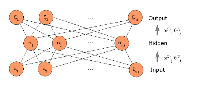
Figure 6: Schematic diagram of a feed-forward neural network.

In practice, it turns out to be convenient to rescale both the input and the output of the neural network, in such a way that they both take values between $0$ and $1$: this avoids having weights $\omega_{ij}$ whose numerical values span many orders of magnitude. We have explicitly checked independence with respect to reasonable variations of this rescaling.

In short, the neural network outputs the values $\xi_{j}^{(l)}$ as a function of the input values $\xi_{j}^{(1)}$ and the parameters $\omega_{ij}$, $\theta_{i}$. The training of the neural network consists of the determination of the best–fit values of these parameters given a set of input-output patterns (data).

As discussed previously in detail [9], the choice of the architecture of the neural network cannot be derived from general rules and it must be tailored to each specific problem. One can roughly guess the size of the neural network based on rules of thumb, then verify by actual fitting which is the critical size above which results become independent of the size of the networks. Finally, one chooses a size which is somewhat larger than the critical one, in order to make sure that results are unbiased.

In previous work [9], it was found that a neural network with two hidden layers and architecture 4-5-3-1 is adequate for a fit of the nonsinglet structure function $F_{2}(x,Q^{2})$. The neural network has four inputs because it turns out to be more efficient to take simultaneously as input both $x$, $Q^{2}$, and their logs $\ln x$, $\ln Q^{2}$. In the present case, the neural network only fits the nonsinglet quark distribution at the initial scale, so only two input neurons for $x$ and $\ln x$ are required. We then retain the same large architecture, which is surely redundant given that now only a function of a single variable is fitted. This leads us to the architecture 2-5-3-1. Stability of the results upon this choice will be tested in Sect. 6.3.

The neural network with this structure can be used to parametrize the nonsinglet quark distribution directly. However, it turns out to be convenient to actually relate the neural network to the quark distribution through a suitable factor. This can be viewed as preprocessing of the data: if the function to be fitted is known to be dominated by some behavior in a given region, it may be convenient to only fit the deviation from this behavior.

In our case, it is known that the PDF has to satisfy the kinematical constraint $q_{\mathrm{NS}}(x=1,Q_{0}^{2})=0.$ Standard counting rules [32] as well as existing parton fits further suggests that the structure function drops as a power as $x\to 1$ (up to logarithmic corrections): typically $q_{\mathrm{NS}}(x=1,Q_{0}^{2})\mathrel{\mathop{\sim}\limits_{\scriptscriptstyle{x\rightarrow 1}}}(1-x)^{3}.$ This suggests that it might be useful to divide out this expected leading behavior as $x\to 1$. The vanishing constraint at $x=1$ is then implemented automatically, which is more efficient than the solution adopted in previous work [9, 10], where the constraint was adopted by adding a Lagrange multiplier, i.e., in practice, artificial points at $F_{2}(x=1,Q^{2})=0$ with various values of $Q^{2}$.

Furthermore, the output of the neural network is by construction bounded. The last layer is a linear function of its input, which in turn has as its largest value the sum of weights, given that $\xi_{j}^{(n_{l}-1)}$ in turn are bounded, $\xi_{j}^{(n_{l}-1)}\leq 1$, according to Eq. (52). However, both current parton fits as well as Regge theory arguments [32] suggest that $q_{\mathrm{NS}}(x,Q_{0}^{2})$ blows up as $x\to 0$. Even though, of course, this growth is cut off by the fact that the data only extend down to a minimum value of $x$, and not to $x=0$, this behavior leads to substantial variation of the PDF in the measured region as $x$ decreases, and it is therefore advantageous to divide it out.

Therefore, we parametrize the nonsinglet parton distribution as

$$q_{\mathrm{NS}}(x,Q_{0}^{2})={{(1-x)^{3}}\over{x}}{\rm NN}(x)\ ,$$ (53)

where ${\rm NN}(x)$ is the neural network discussed above. Independence of the results on the various choices discussed in this section, in particular architecture and pre-processing, will be checked explicitly and discussed in the next section.

5.2 Training

The procedure of fitting (or training, as it is usually called in the context of neural networks) is based on the minimization of a suitable figure of merit. As discussed in Sect. 2, we fit to each replica of the data a nonsinglet quark distribution by maximum likelihood, i.e. we minimize the error function

$$E^{(k)}\left[{\bf\omega}\right]={{1}\over{N_{\mathrm{dat}}}}\sum_{i,j=1}^{N_{\mathrm{dat}}}\left(F_{i}^{(\mathrm{art})(k)}-F_{i}^{(\mathrm{net})(k)}\right)\left(\left(\mathrm{\overline{cov}}\right)^{-1}\right)_{ij}\left(F_{j}^{(\mathrm{art})(k)}-F_{j}^{(\mathrm{net})(k)}\right),$$ (54)

where $F_{i}^{(\mathrm{net})(k)}$ is determined in terms of the nonsinglet quark distribution at the reference scale $Q_{0}^{2}$ by Eq. (21), and the quark distribution at the reference scale is given by a neural network Eq. (53). The covariance matrix $\mathrm{\overline{cov}}^{(k)}$ is defined in Eq. (10) and it does not include normalization errors, as discussed in Sect. 3.2. Note that $E^{(k)}$ is a property of each individual replica, whereas the quality of the global fit is given by the $\chi^{2}$ computed from the averages over the sample of trained neural networks, namely

$$\chi^{2}={{1}\over{N_{\mathrm{dat}}}}\sum_{i,j=1}^{N_{\mathrm{dat}}}\left(F_{i}^{(\exp)}-\left\langle F_{i}^{(\mathrm{net})}\right\rangle_{\mathrm{rep}}\right)\left(\left(\mathrm{cov}\right)^{-1}\right)_{ij}\left(F_{j}^{(\exp)}-\left\langle F_{j}^{(\mathrm{net})}\right\rangle_{\mathrm{rep}}\right),$$ (55)

where now the covariance matrix, defined in Eq.( 4), includes normalization uncertainties.

The error function Eq. (54) can be minimized with a variety of techniques, including standard steepest–descent in the space of parameters. The back-propagation method, which was used in Refs. [9, 10] and is often advantageous for neural network training, cannot be adopted here because the measured quantity (the observed value of the structure function) depends non-locally on the neural network, i.e. it depends on the value of the parton distribution for several values of the input variable $x$. It turns out to be convenient to use a genetic algorithm [33] as a minimization method, as already done in Refs. [10, 11].

The genetic algorithm applied to our problem works in the following way, for each replica and repeating the whole procedure for each replica, i.e. $N_{\mathrm{rep}}$ times (we shall omit for simplicity the index $k$ which identifies the individual replica). The state of the neural network is represented by the weight vector

$${\bf\omega}=\left(\omega_{1},\omega_{2},\ldots,\omega_{N_{\mathrm{par}}}\right)\ .$$ (56)

where each element $\omega_{i}$ corresponds to a weight $\omega^{(l)}_{ij}$ or threshold $\theta_{i}$, and $N_{\mathrm{par}}$ indicates the total number of weights nd thresholds. A set of $N_{\mathrm{mut}}$ copies of the state vector is then generated. Minimization is performed in steps usually referred to as generations (training cycles in ref .[10]). At each generation, a new set of copies of the weight vectors is obtained by means of two operations. First (mutation) a randomly chosen element of the state vector ${\bf\omega}$) is replaced by a new value, according to the rule

$$\omega_{k}\to\omega_{k}+\eta\left(r-{{1}\over{2}}\right)\ ,$$ (57)

where $r$ is a uniform random number between 0 and 1 and $\eta$ (mutation rate) is a free parameter of the minimization algorithm which can be optimized either for the given problem, or dynamically during the minimization. Second (selection) a set of vectors with low values of the error Eq.( 54) are selected out of the total population of $N_{\mathrm{mut}}$ individuals, and use to replace the original vector. The simplest option is to select the $N_{\mathrm{sel}}<N_{\mathrm{mut}}$ vectors with lowest error. Methods based on probabilistic selection, such as those used Ref. [10], explore more efficiently the space of possible mutations. Moreover, in order to avoid the local minima and increase the training speed, we have introduced multiple mutations. Specifically, we have found that one additional mutation with probability 50% and two additional mutations with probability 20% produce a significant improvement of the convergence rate.

The procedure is iterated until the vector with smallest value of the error function of the set for each generation meets a suitable convergence criterion, to be discussed in the next subsection. Note that at each generation the value of the error function never increases. The main advantage of genetic minimization is that it works on a population of solutions, rather than tracing the progress of one point through parameter space. Thus, many regions of parameter space are explored simultaneously, thereby lowering the possibility of getting trapped in local minima. Usually, this procedure is further supplemented by crossing within the chains of mutated parameters (see e.g. Ref. [10]). However, this is not necessary in our case since, thanks to a dedicated preprocessing, mutations alone are enough to reach satisfactory minima. Moreover, the use of Monte Carlo replicas should avoid hitting the same minimum twice.

Here, genetic minimization is applied to an initial set of parameters chosen at random. In fact, in order to fully explore the space of parameters, it turns out to be advantageous to first choose at random the range of parameters, and then their values in this range. In practice, the range is chosen at random between

$$\left[-\left\langle\omega\right\rangle-\sigma_{\omega},\left\langle\omega\right\rangle+\sigma_{\omega}\right]\ ,$$ (58)

and

$$\left[-\left\langle\omega\right\rangle+\sigma_{\omega},\left\langle\omega\right\rangle-\sigma_{\omega}\right]\ ,$$ (59)

where $\left\langle\omega\right\rangle$ and $\sigma_{\omega}$ are the average and variance of the weights computed from the set of best-fit networks obtained in a previous fit. The value of the mutation rate is chosen to be $\eta=8$, and the probabilistic algorithm of Ref. [9] is adopted. While these choices are optimized to obtain fast convergence, we have checked that they do not influence the final results.

Finally, because we have to deal with data sets coming from different experiments and with different features, it turns out to be advantageous to adopt weighted training, in order to ensure that the fit to all experiments is of comparable quality. To this purpose [10], more weight is given to experiments with a larger value of $E$. Namely, the function $E_{\mathrm{min}}$ to be minimized is given by

$$E_{\mathrm{min}}={{1}\over{N_{\mathrm{dat}}}}\sum_{j=1}^{N_{\rm exp}}p_{j}N_{\mathrm{dat},j}E_{j}\ ,$$ (60)

where $N_{\mathrm{dat},j}$ is the number of data points and $E_{j}$ the value of the error function defined in Eq. (54) but restricted to the points coming from the $j-th$ experiment, and the weights $p_{j}$ are adjusted dynamically according to

$$p_{j}=\left({{E_{j}}\over{E_{\mathrm{max}}}}\right),$$ (61)

where $E_{\mathrm{max}}$ is the highest amongst the values of $E_{j}$. In order to avoid introducing artificial instabilities, the re-weighting is only used if the ratio on the right–hand side of Eq. (61) differs significantly from one. In practice, no reweighting is implemented if $c_{\rm min}<E_{NMC}/E_{BCDMS}<c_{\rm max}$, with $c_{\rm min}=0.78$ and $c_{\rm max}=1.22$.

5.3 Stopping

As we explained already, the crucial feature which guarantees a bias-free fit is the possibility of stopping the training not at the lowest value of the figure of merit (which might depend on the functional form of the fitting function), but rather when suitable criteria are met. These criteria should single out the point where the fit reproduces the information contained in the data, but not the statistical noise. Namely, the best fit should have the lowest possible value of the figure of merit compatible with the requirement of not overlearning, i.e. not fitting statistical fluctuations. In previous work [9, 10], this was done by determining an optimal training length. The present case is more subtle, because on the one hand the fitted function is much more constrained by the data, on the other hand, the quantity which is being fitted is not directly observable. This makes it harder to distinguish overlearning from an actual improvement in the fit.

We therefore adopt the following criterion. We separate the data set into two disjoint sets. We then minimize the error function, Eq. (54) computed only with the data points of the first set (training set, henceforth). During the minimization process, we compute the error function from the data of the second set (validation set, henceforth). The best fit has been reached when the validation error function ceases to decrease. Overlearning, in particular, corresponds to a situation where the training error function keeps decreasing while the validation one does not, thereby signaling that the fit is merely reproducing the fluctuations of the specific training set. The procedure is reliable and it does not lead to loss of information if both the training and the validation set reproduce the features of the full data set. This can be simply achieved on average by choosing a different random partition for each replica of the data, and then checking that the number of replicas is sufficiently large. Similar methods have been widely used in various applications of neural networks, and in high–energy physics e.g. in Ref. [34].

In practice, we implement this stopping criterion as follows. We define a training fraction $f_{\mathrm{tr}}=N_{\mathrm{tr}}/N_{\mathrm{dat}}$ (with default value $f_{\mathrm{tr}}=0.5$) and for each replica we select at random a fraction $f_{\mathrm{tr}}$ of points for each experiment, which we use for training, while the remaining points are assigned to a validation set. We then compute separately the corresponding training and validation covariance matrices. The training error function $E^{(k)}_{\mathrm{tr}}$ Eq. (54) is minimized using a genetic algorithm, and at each generation of the genetic minimization the validation error function $E^{(k)}_{\mathrm{val}}(l)$ is computed as a function of the generation index $l$. Having chosen a fixed fraction of points separately for each experiment allows for weighted training. Both $E^{(k)}_{\mathrm{tr}}$ and $E^{(k)}_{\mathrm{val}}(l)$ are computed neglecting cross–correlations between data in the validation and the training set: we have verified that this is a small correction anyway.

We then let the training proceed at least until $E^{(k)}_{\mathrm{tr}}$ has reached the threshold value $E^{(k)}_{\mathrm{tr}}=E_{\mathrm{min}}$. We choose as default the value $E_{\mathrm{min}}=3$ . This ensures that the training does not stop due to fluctuations in the early stages. Beyond this point, i.e. if $E^{(k)}_{\mathrm{tr}}\leq E_{\mathrm{min}}$, the training is stopped at the $l$-th generation if the training error function decreases,

$${{\left\langle E_{\rm tr}(l)\right\rangle}\over{\left\langle E_{\rm tr}(l-N_{\rm sm})\right\rangle}}<1$$ (62)

while the validation error function

$${{\left\langle E^{(k)}_{\mathrm{val}}\left(l\right)\right\rangle}\over{\left\langle E^{(k)}_{\mathrm{val}}\left(l-N_{\mathrm{sm}}\right)\right\rangle}}\geq 1\ ,$$ (63)

where

$$\left\langle E^{(k)}_{\mathrm{val}}\right\rangle\left(l\right)\equiv{{1}\over{N_{\mathrm{sm}}}}\sum_{i=l-N_{\mathrm{sm}}+1}^{l}E^{(k)}_{\mathrm{val}}(i)\ ,$$ (64)

with $E^{(k)}_{\mathrm{val}}(i)$ the validation error function for the $i-$th GA generation, and similarly for the training error. In other words, the training is stopped if the value of the validation error function averaged over $N_{\mathrm{sm}}$ generation starts increasing, while the training error function decreases. This last condition must be imposed (despite the fact that with a genetic algorithm the figure of merit always decreases) because of weighted training: when the weighting is readjusted the error function could increase locally. We take $N_{\mathrm{sm}}=4$ as a default value. This averaging of the figures of merit along the training is analogous to the determination of moving averages, widely used especially in financial dynamics.

Finally, we have introduced an upper length to the training process, i.e. a maximum number of generation $N_{\mathrm{gen}}$, chosen to correspond to a very long training such that the validation error function is no longer expected to decrease. The default value is $N_{\mathrm{gen}}=800$. In practice, the criterion condition (63) was always met well before this point except in a tiny number of cases.

6 Results

We present our best-fit result for the nonsinglet quark distribution and its statistical features, and in particular we show that it provides a consistent estimate of both central values and errors. We will then show its stability upon variation of the fitting procedure.

6.1 Next-to-leading order results: central values

Figure 7: The best-fit NLO nonsinglet quark distribution $q_{\rm\mathrm{NS}}(x,Q_{0}^{2})$ in the large-$x$ region. The MRST, CTEQ and Alekhin determinations are also shown for comparison. In this and subsequent plots of $q_{\rm\mathrm{NS}}$ we take $Q^{2}=Q_{0}^{2}=2$ GeV².

Figure 8: The best-fit NLO nonsinglet quark distribution $q_{\rm\mathrm{NS}}(x,Q_{0}^{2})$ in the small-$x$ region. The MRST, CTEQ and Alekhin determinations are also shown for comparison.

The result obtained from a set of $N_{\mathrm{rep}}=1000$ neural networks trained to replicas of the data with the method described above, using the NLO expressions of the coefficient function and anomalous dimension is displayed in Figs. 7 and  8. The error band corresponds to a one–sigma contour. The distributions of values of the error function $E$ Eq. (54) for the training and validation samples are displayed in Fig. 9. These distributions are poissonian (gaussian) to good approximation, and both are peaked around a similar value, thereby showing that the quality of the fit for points included or not included in the fit is equally good. The distribution of training lengths is shown in Fig. 10. It is poissonian to good approximation, and it shows that convergence is reached after a small number of generations of the genetic algorithm, much smaller than the maximum $N_{\mathrm{gen}}$ which is only reached in a tiny number of cases.

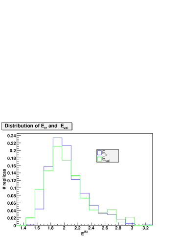
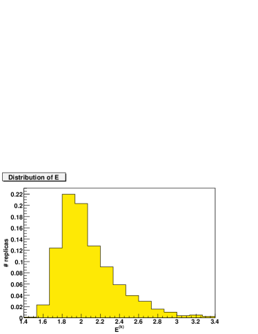
Figure 9: Distribution of values of the error function $E$ Eq. (54) at the stopping point for the training and validation samples (left), and for the full data sample (right).

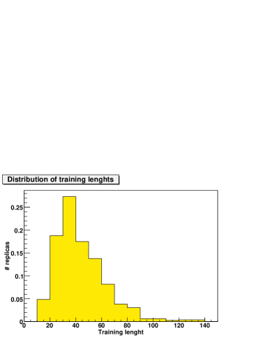
Figure 10: Distribution of training lengths.

The distribution of values of the error function $E$ Eq. (54) for the total data set is displayed in Fig. 9, while the statistical properties of the fit are summarized in Table 6. Note that, because the quantities listed in the table characterize the comparison of the fit to the data (see Appendix B for the definitions), they are determined from the structure function $F_{2}^{\rm\mathrm{NS}}$ rather than the quark distribution itself. The error functions of each fit are distributed to good approximation in a gaussian way about the value $\langle E\rangle=2.27$ given in Table 6. A value $\langle E\rangle\approx 2$ is expected for a good fit because if errors are correctly estimated, the average standard deviation of true values about the measured value should equal the total uncertainty, but replicas are generated about the measured values so their average standard deviation about the true values should be twice the total uncertainty. However, the fit to each individual replica should be closer to the true value, because of the availability of many data points at various values of $Q^{2}$ which are combined by the fit. Indeed, the average error of the fit is much smaller than the average experimental error: $\left\langle\sigma^{(\mathrm{net})}\right\rangle_{\mathrm{dat}}\ll\left\langle\sigma^{(\exp)}\right\rangle_{\mathrm{dat}}$ (see Table 6).

The fact that the figure of merit for the global fit Eq. (55) takes the value $\chi^{2}\approx 1$ shows that the central value of the fit, after averaging over replicas, is distributed about the measured values as one expects of the correct distribution of true values, namely, with variance equal to the experimental error (which is much larger than the error on the fit itself as we just discussed). Note that, strictly speaking, the total number of independent degrees of freedom is somewhat smaller than the total number of points. However, the number of effective free parameters of the neural network is rather smaller than the total number of weights and thresholds, because our choice of stopping criterion ensures that the neural network is redundant. Hence, the number of degrees of freedom is at most by a few percent smaller than $N_{\mathrm{dat}}$ (and the correctly estimated $\chi^{2}$ accordingly larger), which is smaller than the uncertainty on $\chi^{2}$ due to statistical fluctuations, which is of order of $N_{\mathrm{dat}}^{-1/2}$. However, as a consequence of this, we expect the value of $\chi^{2}/N_{\mathrm{dat}}$ to be systematically lower than one by a few percent for an optimal fit. This expectation will be borne out by our results.

	Total	NMC	BCDMS
$\chi^{2}_{\mathrm{tot}}$	0.75	0.72	0.78
$\left\langle E\right\rangle$	2.27	1.99	2.52
$r\left[F_{2}^{\mathrm{NS}}\right]$	0.81	0.66	0.95
$\left\langle\sigma^{(\exp)}\right\rangle_{\mathrm{dat}}$	0.011	0.017	0.006
$\left\langle\sigma^{(\mathrm{net})}\right\rangle_{\mathrm{dat}}$	0.006	0.009	0.004
$r\left[\sigma^{(\mathrm{net})}\right]$	0.59	-0.04	0.86
$\left\langle\rho^{(\exp)}\right\rangle_{\mathrm{dat}}$	0.11	0.39	0.16
$\left\langle\rho^{(\mathrm{net})}\right\rangle_{\mathrm{dat}}$	0.46	0.42	0.50
$r\left[\rho^{(\mathrm{net})}\right]$	0.15	0.25	0.04
$\left\langle{\rm cov}^{(\exp)}\right\rangle_{\mathrm{dat}}$	$8.6~{}10^{-6}$	$1.0~{}10^{-5}$	$7.2~{}10^{-6}$
$\left\langle{\rm cov}^{(\mathrm{net})}\right\rangle_{\mathrm{dat}}$	$2.1~{}10^{-5}$	$3.8~{}10^{-5}$	$6.9~{}10^{-6}$
$r\left[{\rm cov}^{(\mathrm{net})}\right]$	0.24	0.23	0.57

Table 6: Statistical estimators for the final sample of $N_{\mathrm{rep}}=1000$ neural networks, both for the total data points and for the individual experiments incorporated in the fit (NMC and BCDMS).

We conclude that the central fit is correctly estimated.

6.2 Next-to-leading order results: uncertainties

Because experimental errors are much larger than the error on the fit, the values of $\left\langle E\right\rangle$ and $\chi^{2}$ discussed in Sect. 6.1 do not test for the accuracy of the one–sigma error band on the central fit. We can check for the correctness of the latter by studying the fluctuation of predictions obtained from different sets of replicas. To this purpose, we note that we can view the prediction $q_{i}$ obtained for the central values of the quark distribution by averaging over $N_{\mathrm{rep}}$ replicas, as a random variable, whose variance is given by

$$V[q_{i}]={{\sigma^{2}_{q_{i}}}\over{N_{\mathrm{rep}}}},$$ (65)

in terms of the variance $\sigma^{2}_{q_{i}}$ of the set of replicas. We can define an average distance $d[q]$ as the root–mean square difference between values of $q_{i}$ obtained by averaging over different set of replicas, normalized to the variance Eq. (65) (see appendix B). If the error on $q$ is correctly estimated, the average of $d[q]$, determined for different points, must approach one. We can similarly view the standard deviation of each data point $\sigma^{2}_{q_{i}}$, and test for their statistical accuracy by computing the corresponding distances.

$N_{\mathrm{rep}}$	10	100	500
$\left\langle d\left[q\right]\right\rangle_{\mathrm{dat}}$	1.02	0.96	0.92
$\left\langle d\left[q\right]\right\rangle_{\mathrm{extra}}$	1.11	0.99	0.85
$\left\langle d\left[\sigma_{q}\right]\right\rangle_{\mathrm{dat}}$	0.93	0.88	0.93
$\left\langle d\left[\sigma_{q}\right]\right\rangle_{\mathrm{extra}}$	1.13	0.97	0.91

Table 7: Stability estimators as a function of the number of trained replicas $N_{\mathrm{rep}}$.

Hence, we test for accuracy of estimates of errors and correlations by computing this distance for the quark distribution $q_{i}$ (determined as an average over neural networks) and the error on it $\sigma^{2}_{q_{i}}$ (determined as variance of the networks). The distance is determined between results obtained from a set of $N_{\rm rep}$ replicas each. The computation is performed for 14 points linearly spaced in $x$ in the data region ($0.05\leq x\leq 0.75$) and then averaged, and similarly for the same number of points logarithmically spaced in the extrapolation region ($10^{-3}\leq x\leq 10^{-2}$). In order for the result to be significant we must make sure that its standard deviation $\sigma_{d}$ is not too large. However, because $d$ is a standard deviation itself (normalized to its expected value), $\sigma_{d}$ only scales as $n^{-1/4}$ with the number of points $n$, so $\sigma_{d}\sim 0.5$. On the other hand, increasing the number of points will not help because, of course, two values of $q(x)$ and $q(x^{\prime})$ are highly correlated when $x$ and $x^{\prime}$ are close to each other. Thus, we obtain stability by repeating the computation for different random choices of two sets of $N_{\mathrm{rep}}$ replicas among the starting $2N_{\mathrm{rep}}$ ones, and averaging the results, which reduces the standard deviation according to Eq. (65). We average over 1000 sets, so that $\sigma_{d}\sim 0.01$.

Results with increasing values of $N_{\mathrm{rep}}$ are shown in Table 7. The distance already converges to the expected value of one, to percent accuracy, when $N_{\rm rep}=10$. Note that, because of Eq. 65, the expected distance decreases as ${{1}\over{\sqrt{N_{\rm rep}}}}$: the stability of the result we get when the number of replicas is further increased from 100 to 500 shows that this behaviour is indeed observed in our sample of neural networks.

6.3 Stability upon variation of the neural network structure

After verifying that our results are statistically consistent, we wish to check that they do not depend on the details of the fitting procedure. We do this by determining the distance discussed in Sect. 6.2, but now computed for a pair of fits which differ in fitting procedure. Independence is verified if the distance equals its value predicted on statistical grounds (i.e. that which would be obtained from pairs of replicas coming from the same fit). Specifically, the computation is done by taking $N_{\mathrm{rep}}=50$, and then averaging over 1000 different choices of these 50 replicas among a total set of $N_{\mathrm{rep}}=100$ replicas. Note that, because of Eq. 65, this verifies independence of the fitting procedure to an accuracy which is by a factor $\sqrt{50}$ smaller than the uncertainty on the central value.

Architecture	2-4-3-1
$\chi^{2}$	0.75
$\left\langle d\left[q\right]\right\rangle_{\mathrm{dat}}$	0.9
$\left\langle d\left[q\right]\right\rangle_{\mathrm{extra}}$	0.9
$\left\langle d\left[\sigma_{q}\right]\right\rangle_{\mathrm{dat}}$	0.9
$\left\langle d\left[\sigma_{q}\right]\right\rangle_{\mathrm{extra}}$	1.4

Table 8: Independence of the architecture of the neural networks.

The first check is to verify that our results are indeed independent of the neural network architecture. We have compared the results of the fit with the reference architecture 2-5-3-1 with the results of a similar fit with a smaller neural network architecture 2-4-3-1. The result of this comparison can be seen in Table 8. This confirms that we have achieved independence of the number of parameters used, both in the data and in the extrapolation region, a property that is very difficult to achieve in standard parton fits with fixed functional form.

Next, we estimate the dependence of the results on the different kind of preprocessing, namely, on the values of the exponents $m$ and $n$

$$q_{\mathrm{NS}}(x,Q^{2}_{0})={{(1-x)^{m}}\over{x^{n}}}NN(x)\ ,$$ (66)

when varied about the default values $m=3$ and $n=1$. In Table 9 we display the dependence of the $\chi^{2}$, computed from a set of $N_{\mathrm{rep}}=100$ replicas, and the stability of the fit when $1\leq m\leq 4$ (with $n=1$ fixed) and when $0.5\leq n\leq 1.25$ (with $m=3$ fixed). It appears that the fit is reasonably stable if $2.5\leq m\leq 3.5$ and $0.5\leq n\leq 1.25$: central values in the data region fluctuate less than three $\sigma$ while the uncertainty is stable. The central fit starts changing in a statistically significant way when $m$ and $n$ are varied outside these bounds. However, in such case the quality of the fit, as measured by the $\chi^{2}$, deteriorates considerably. Hence, we conclude that the fit is independent of the choice of $m,n$ provided these are kept within a range which allows for an optimal quality of the fit.

Fits within the stability region of the preprocessing exponents are compared in Fig. 11. Stability of central values and errors in the data and extrapolation region are apparent. Note that the distance Eq. (65) is computed with $N_{\mathrm{rep}}=50$, hence the distance of the central values equals about 15% of the error band displayed in the plot.

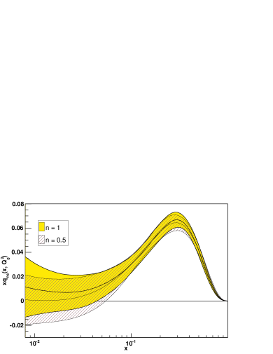
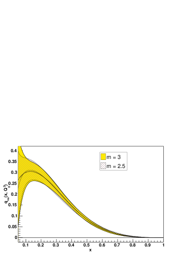
Figure 11: Dependence of the results on the preprocessing exponents $m$, $n$, Eq. (66)

$(m,n)$	(1,1)	(2,1)	(2.5,1)	(3,1)	(3.5,1)	(4,1)
$\chi^{2}$	0.85	0.94	0.83	0.75	0.77	0.84
$\left\langle d\left[q\right]\right\rangle_{\mathrm{dat}}$	4.5	4.6	2.9	-	3.3	6.1
$\left\langle d\left[q\right]\right\rangle_{\mathrm{extra}}$	0.8	0.8	0.8	-	0.8	0.8
$\left\langle d\left[\sigma_{q}\right]\right\rangle_{\mathrm{dat}}$	2.0	1.7	1.2	-	1.2	1.5
$\left\langle d\left[\sigma_{q}\right]\right\rangle_{\mathrm{extra}}$	1.9	2.0	1.3	-	1.0	1.1

$(m,n)$	(3,0.5)	(3,0.75)	(3,0.9)	(3,1)	(3,1.1)	(3,1.25)
$\chi^{2}$	0.79	0.77	0.74	0.75	0.76	0.77
$\left\langle d\left[q\right]\right\rangle_{\mathrm{dat}}$	2.5	2.1	1.0	-	1.2	1.6
$\left\langle d\left[q\right]\right\rangle_{\mathrm{extra}}$	1.2	0.8	0.9	-	1.9	1.5
$\left\langle d\left[\sigma_{q}\right]\right\rangle_{\mathrm{dat}}$	1.3	1.3	0.9	-	1.0	1.3
$\left\langle d\left[\sigma_{q}\right]\right\rangle_{\mathrm{extra}}$	1.0	1.3	1.2	-	1.8	2.5

Table 9: Dependence on the preprocessing exponents.

7 Theoretical uncertainties

So far we have checked that our fit reproduces correctly the information contained in the data, and thus that the error band computed from it is statistically consistent. A priori, there are further sources of theoretical error related to use of perturbative QCD in the fitting procedure: specifically those related to higher order perturbative corrections and to higher twist terms. In this section we will show that these theoretical errors are in fact negligible. All tests in this section, as in Sect. 6.3 are done by computing the $\chi^{2}$ from a set of 100 replicas, and the distance by taking $N_{\mathrm{rep}}=50$, and then averaging over 1000 different choices of these 50 replicas among a total set of $N_{\mathrm{rep}}=100$ replicas.

7.1 Dependence on kinematic cuts

We first discuss the dependence of results for the nonsinglet parton distribution $q_{\mathrm{NS}}(x,Q^{2})$ on the kinematical cut in $Q^{2}$. In Fig. 12 and Table 10 we compare results obtained when the value $Q_{\min}^{2}$ is raised to $Q_{\mathrm{min}}^{2}=9$ GeV², to results obtained with the default value $Q_{\mathrm{min}}^{2}=3$ GeV². Removing the data points in the region 3 GeV${}^{2}\leq Q^{2}\leq 9$ GeV² eliminates the bulk of the NMC measurements, i.e. (see Fig. 2) essentially all data with $x<0.1$.

As a consequence, uncertainties increase sizably in the small-$x$ region. However, results are remarkably stable in the large $x$ region. In Tab. 10 we compare results in three different kinematical regions: where the two fits with different kinematical cuts have data (region I, $0.2\leq x\leq 0.75$), where only the fit with $Q^{2}_{\mathrm{min}}=3$ GeV² has data (region II, $0.05\leq x\leq 0.1$) and finally the region where both fits extrapolate (region III, $x\leq 10^{-2}$). Not only in region I the two fits agree completely, but even in region II, whereas the uncertainty bands increases considerably, the central fit is essentially unaffected. This proves the remarkable stability of our results.

	$x\leq 10^{-2}$	$5~{}10^{-2}\leq x\leq 0.1$	$0.2\leq x\leq 0.75$
$\left\langle d\left[q\right]\right\rangle$	0.6	0.8	0.9
$\left\langle d\left[\sigma\right]\right\rangle$	2.7	3.2	1.4

Table 10: Comparison of fits with different kinematical cuts. The fit with $Q_{\mathrm{min}}^{2}=3~{}\mathrm{GeV}^{2}$ (reference) is compared to the fit with $Q_{\mathrm{min}}^{2}=9~{}\mathrm{GeV}^{2}$ in three different regions of $x$.

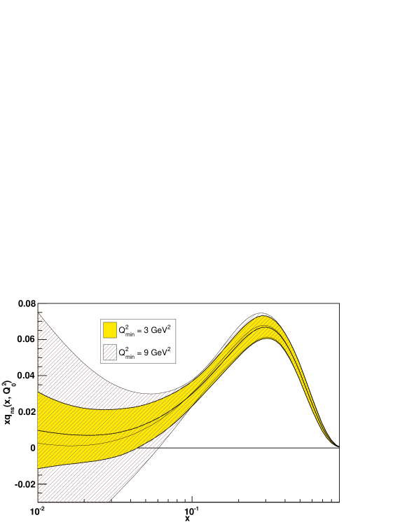
Figure 12: Results for $xq_{\mathrm{NS}}(x,Q_{0}^{2})$ with two different kinematical cuts in $Q^{2}$.

7.2 Higher twists

Fit	$Q_{\min}^{2}=3~{}\mathrm{GeV}^{2}$+HT	$Q_{\min}^{2}=5~{}\mathrm{GeV}^{2}$	$Q_{\min}^{2}=5~{}\mathrm{GeV}^{2}$+HT
$\chi^{2}$	0.76	0.79	0.78
$\left\langle d\left[q\right]\right\rangle_{\mathrm{dat}}$	2.9	0.8	3.2
$\left\langle d\left[q\right]\right\rangle_{\mathrm{extra}}$	1.4	0.8	0.9
$\left\langle d\left[\sigma_{q}\right]\right\rangle_{\mathrm{dat}}$	1.2	1.5	1.9
$\left\langle d\left[\sigma_{q}\right]\right\rangle_{\mathrm{extra}}$	1.3	1.8	2.3

Table 11: Results of the higher-twist analysis. Stability is computed relative to the default NLO fit.

We now test for the possible role of higher twist terms, on top of the target–mass corrections which are already included in our default fit as discussed in Sect. 4.4. To this purpose, we switch on a twist–four contribution according to Eq. (49), and parametrize $HT(x)$ with a 1-2-1 neural network. In Table 11 we compare the $\chi^{2}$ obtained by including this higher twist term to that obtained by raising the cut in $Q^{2}$. On the one hand, we see that including higher-twist corrections without raising the $Q^{2}$ does not lead to any improvement in the quality of the fit. On the other hand, we see that if the $Q^{2}$ is raised, the $\chi^{2}$ also does not improve — in fact it deteriorates slightly, in a way which is unaffected by the inclusion of higher twist terms.

We take the lack of improvement in $\chi^{2}$ when either the cut is raised, or higher twist terms are included, as an indication of the fact that there is no evidence whatsoever for higher twist terms even with our lower default cut. The slight deterioration in $\chi^{2}$ when the $Q^{2}$ cut is raised is likely to be related to the fact that experimental uncertainties in the small–$Q^{2}$ region (i.e. experimental uncertainties on NMC data) are somewhat overestimated.

We conclude that there is no evidence for higher twists for nonsinglet $F_{2}^{\mathrm{NS}}$ data with $Q^{2}>3$ GeV².

7.3 Higher orders and the value of the strong coupling

So far we have discussed the determination of the nonsinglet parton distribution through a NLO analysis. We now compare these results to those obtained at one less and one more perturbative order. Hence, we produce a full LO fit, with $\alpha_{s}\left(M_{Z}^{2}\right)=0.130$ and a full NNLO fit, with $\alpha_{s}\left(M_{Z}^{2}\right)=0.115$. The results of these fits are compared to the NLO ones in Table 12. No variation of the quality of the fit is found between different perturbative orders: the values of $\chi^{2}$ and $\left\langle\sigma^{(\mathrm{net})}\right\rangle_{\mathrm{dat}}$ are unaffected by the perturbative order at which the computation is performed. Indeed, only very small improvements of the $\chi^{2}$ when going from LO to NLO and NNLO have been found in recent nonsinglet fits [35, 36].

This means that the effects of higher–order corrections are entirely reabsorbed in a change of the initial quark distribution. This change is statistically significant when going from LO to NLO: the central values moves by $d\approx 10$ (see Tab. 12), i.e. by about half the error on the central value. Indeed, we have verified that if Tab. 12 is recomputed using a set of $N_{\mathrm{rep}}=50$ replicas, we get $\left\langle d\left[q\right]\right\rangle_{\mathrm{dat}}=3.2$ for the LO fit. This means that the LO and NLO central values differ by a fixed amount, independent of the number of replicas used to determine the central value, therefore if we normalize to the standard deviation Eq. 65 the result grows as $\sqrt{N_{\mathrm{rep}}}$. No statistically significant difference in central values is observed when going from NLO to NNLO. Hence, our result supports the conclusion [35] that nonsinglet data are insufficient to provide evidence for higher–order perturbative corrections. These results are apparent in Fig. 13, where the LO, NLO and NNLO fits are compared.

Perturbative order	LO	NLO	NNLO
$\chi^{2}$	0.751	0.750	0.754
$\left\langle d\left[q\right]\right\rangle_{\mathrm{dat}}$	10.2	-	2.6
$\left\langle d\left[q\right]\right\rangle_{\mathrm{extra}}$	1.2	-	1.2
$\left\langle d\left[\sigma_{q}\right]\right\rangle_{\mathrm{dat}}$	2.2	-	3.0
$\left\langle d\left[\sigma_{q}\right]\right\rangle_{\mathrm{extra}}$	1.3	-	1.3
$\left\langle\sigma^{(\mathrm{net})}\right\rangle_{\mathrm{dat}}$	$0.51~{}10^{-2}$	$0.62~{}10^{-2}$	$0.49~{}10^{-2}$

Table 12: Quantitative comparison of fits at different perturbative orders. The distance is computed relative to the NLO fit using a set of $N_{\mathrm{rep}}=500$ replicas.

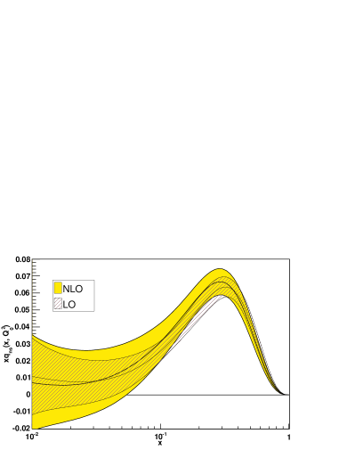
Figure 13: Comparison of a LO fit (left) and a NNLO fit (right) to the reference NLO fit.

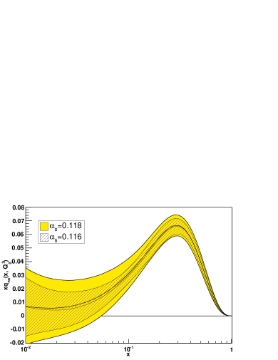
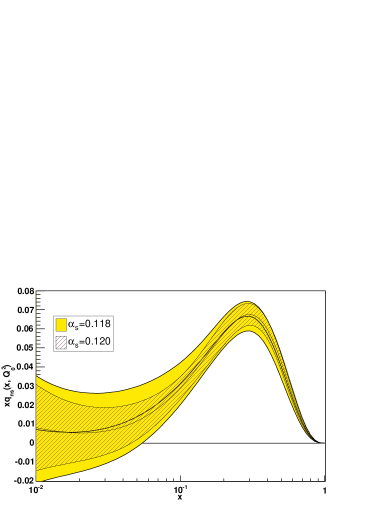
Figure 14: Comparison of the reference fit to fits with a lower (left) or higher (right) value of $\alpha_{s}\left(M_{Z}^{2}\right)$

$\alpha_{s}(M_{Z}^{2})$	0.116	0.118	0.120
$\chi^{2}$	0.743	0.750	0.744
$\left\langle d\left[q\right]\right\rangle_{\mathrm{dat}}$	3.8	-	4.1
$\left\langle d\left[q\right]\right\rangle_{\mathrm{extra}}$	0.8	-	0.7
$\left\langle d\left[\sigma_{q}\right]\right\rangle_{\mathrm{dat}}$	1.6	-	2.4
$\left\langle d\left[\sigma_{q}\right]\right\rangle_{\mathrm{extra}}$	1.4	-	1.5
$\left\langle\sigma^{(\mathrm{net})}\right\rangle_{\mathrm{dat}}$	$0.52~{}10^{-2}$	$0.62~{}10^{-2}$	$0.53~{}10^{-2}$

Table 13: Quantitative comparison of fits at NLO with different values of $\alpha_{s}(M_{Z}^{2})$.

The fact that NLO corrections have a negligible impact on the fit suggests that the fit is only weakly dependent on the value of $\alpha_{s}\left(M_{Z}^{2}\right)$. We have repeated our NLO fit while varying the value of $\alpha_{s}\left(M_{Z}^{2}\right)$ by one sigma about its central value, i.e. with $\alpha_{s}\left(M_{Z}^{2}\right)=0.116$ and $\alpha_{s}\left(M_{Z}^{2}\right)=0.120$. Comparison to the central fit (Fig. 14 and Tab. 13) shows that the variation of the central fit due to the change in $\alpha_{s}\left(M_{Z}^{2}\right)$ in this range has marginal statistical significance: $\left\langle d\left[q\right]\right\rangle_{\mathrm{dat}}\sqrt{N_{\mathrm{dat}}}\approx 0.2$, i.e., the central fit moves by about a fifth of a standard deviation when $\alpha_{s}\left(M_{Z}^{2}\right)$ is varied in this range. This variation, though small, appears to be stable: if 50 replicas are used we get $\left\langle d\left[q\right]\right\rangle_{\mathrm{dat}}=1.3$ for $\alpha_{s}\left(M_{Z}^{2}\right)=0.116$ and $\left\langle d\left[q\right]\right\rangle_{\mathrm{dat}}=1.1$ for $\alpha_{s}\left(M_{Z}^{2}\right)=0.120$, corresponding to the same value of $\left\langle d\left[q\right]\right\rangle_{\mathrm{dat}}\sqrt{N_{\mathrm{dat}}}\approx 0.2$. The variation of the $\chi^{2}$ in this range is also marginal and it does not show a clear trend. We conclude that a NLO determination of $\alpha_{s}$ based on nonsinglet data only is in principle possible, but it is necessarily affected by an uncertainty which is sizably larger than the error $0.002$ on the PDG average. A smaller value for this uncertainty would be a likely indication of an underestimate of the uncertainty related to the choice of parton parametrization.

8 The structure function

We finally turn to results for the physically measurable structure function $F_{2}^{\rm\mathrm{NS}}(x,Q^{2})$, which we compare to the data and to results obtained in various other approaches.

8.1 Comparison to data and other parton fits

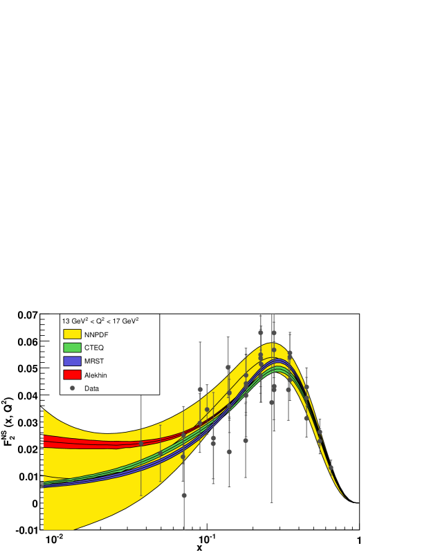
Figure 15: Our NLO determination of the nonsinglet structure function $F_{2}^{\mathrm{NS}}(x,Q^{2})$ at fixed $Q^{2}=15$ GeV² compared to all data with $13\leq Q^{2}\leq 17$ GeV². Determinations by other groups are also shown.

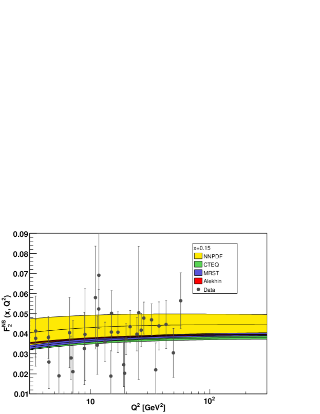
Figure 16: Our NLO determination of the nonsinglet structure function $F_{2}^{\mathrm{NS}}(x,Q^{2})$ as a function of $Q^{2}$ for $x=0.15$, compared to all data in the range $0.13\leq x\leq 0.17$. Determinations by other groups are also shown.

In Figs. 15 and 16 we show a comparison of our results for the nonsinglet structure function $F_{2}^{\mathrm{NS}}(x,Q^{2})$ as a function of $x$ at fixed $Q^{2}=15$ GeV² compared to all data with $13\leq Q^{2}\leq 17$ GeV², and as a function of $Q^{2}$ at fixed $x=0.15$, compared to all data in the range $0.13\leq x\leq 0.17$. In the same figure, we also show the structure function obtained from the results of the global fits of the CTEQ [5] and MRST [6] collaborations and the fit to deep-inelastic data by Alekhin [4].

The uncertainty in the final structure function is much smaller than that on the data, thanks to the theoretical information from perturbative evolution. Nevertheless, the uncertainty in our determination, especially at small $x$, is rather larger than that found in previous analyses. One may wonder whether this is due to the fact that the global analyses are based on a wider set of data. However, in the small $x$ region, where the difference between the uncertainty on our result and that found by other groups is most striking, none of the data contained in these global fits can constrain $q_{\mathrm{NS}}(x,Q_{0}^{2})$, on top of the data on $F_{2}^{\mathrm{NS}}(x,Q^{2})$ which we also include. This suggests that the smaller error band obtained by these groups may be due to parametrization bias or uncertainty underestimation.

Be that as it may, wheras all available fits are within our error band, our central result disagrees with these fits, which in turn disagree with each other within respective errors, even in the valence region $0.1\leq x\leq 0.3$.

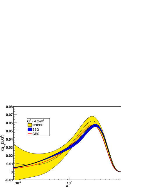
Figure 17: Comparison of our NNLO fit with the results of the nonsinglet fits of Refs. [36] and [35].

Finally, it is interesting to compare our NNLO determination of the nonsinglet parton distribution to the results of some recent NNLO fits to nonsinglet DIS data [35, 36] (see Fig. 17). Results are analogous to those found when comparing to global fits.

8.2 Comparison to neural $F_{2}^{\mathrm{NS}}(x,Q^{2})$

In Ref. [9] the nonsinglet structure function $F_{2}^{\mathrm{NS}}(x,Q^{2})$ was directly parametrized with neural networks as a function of its two arguments, instead of being obtained by evolving a parton distribution. The results of that analysis are compared to the present NLO determination in Fig. 18. The comparison shows that the uncertainty on the determination of Ref. [9] is already smaller than that of the data, because of the requirement of smoothness of the function which is fitted to them, as discussed in detail in Ref. [9]. However, thanks to the extra information from perturbative evolution, the uncertainty is further reduced by a considerable amount when fitting the structure function. Also, it is apparent that thanks to this error reduction, a more detailed determination of the shape of $F_{2}^{\mathrm{NS}}$ is possible. We also display the pull (see Appendix B) between these two determinations, which shows that they are in perfect agreement within one sigma in the region where there are data: whenever the pull increases in modulo above one, no data are available.

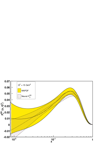
Figure 18: Comparison of the structure function $F_{2}^{\mathrm{NS}}(x,Q^{2})$ obtained from our NLO $q_{\mathrm{NS}}(x,Q_{0}^{2})$ with the NNPDF parametrization of $F_{2}^{\mathrm{NS}}(x,Q^{2})$ at $Q^{2}=15$ GeV²: structure function (left) and pull (right). The pull at $Q^{2}=55$ GeV² is also shown (lower curve at large $x$).

9 Conclusions and outlook

In this paper we have provided a first determination of a parton distribution within an approach based on the use of neural networks coupled to a Monte Carlo representation of the probability density in the space of structure functions.

Our final results take the form of a Monte Carlo sample of neural networks. The nonsinglet parton distribution $q_{\mathrm{NS}}(x,Q_{0}^{2})$ and its statistical moments (errors, correlations and so on) can be determined by averaging over this sample. These results together with driver FORTRAN code can be downloaded from the web site http://sophia.ecm.ub.es/nnpdf/.

The main distinctive features of our determination of the isotriplet quark distribution when compared to that obtained in other fits are the following:

• Our fit is demonstrably independent of the parametrization, and the uncertainty on it has the correct statistical behavior which one expects of an unbiased statistical estimator.

• The uncertainty is greatly reduced in comparison to that on the data, and also to that obtained in fits [9] which do not exploit the constraint of perturbative parton evolution.

• The error band on our result, especially at small $x$, is rather larger than that of other fits, and in fact it includes these other fits even when they disagree with each other.

• The quality of fits at LO, NLO and NNLO is the same: difference in perturbative order can be reabsorbed in the choice of boundary condition.

Our approach is designed to tackle some of the most serious problems that plague current global parton fits, namely, the difficulty of keeping under control the bias due to the choice of parametrization, problems in combining different data sets, and the problem of determining faithfully the uncertainty on the final result. This first application to the determination of a single parton distribution from all structure function data shows that the approach is viable and successful. Its ultimate success or failure will be in its application to a global parton fit from all available data.

Appendix A Large $x$ behavior of the evolution factor

At leading order in $\alpha_{s}\left(Q^{2}\right)$, in the large $x$ limit, the dominant contribution to the evolution kernel comes from the large $N$ limit of the LO anomalous dimension, given by

$$\Gamma(x)=\int_{-i\infty}^{+i\infty}{{dN}\over{2\pi i}}x^{-N}\left({{\alpha_{s}\left(Q^{2}\right)}\over{\alpha_{s}\left(Q^{2}_{0}\right)}}\right)^{C_{F}\ln N/\pi\beta_{0}}.$$ (67)

The inverse Mellin transformation can be performed to all logarithmic orders using the formulas of Ref. [37], with the result

$$\Gamma(x) = \sum_{n=1}^{\infty}{{\Delta^{(n-1)}(1)}\over{(n-1)!}}\left[{{1}\over{1-x}}{{d^{n}}\over{d\ln^{n}(1-x)}}\left({{\alpha_{s}\left(Q^{2}\right)}\over{\alpha_{s}\left(Q^{2}_{0}\right)}}\right)^{C_{F}\ln(1-x)/\pi\beta_{0}}\right]_{+}+\mathcal{O}((1-x)^{0})$$ (68)

$$= \Delta\left({{C_{F}}\over{\pi\beta_{0}}}\ln\left({{\alpha_{s}\left(Q^{2}_{0}\right)}\over{\alpha_{s}\left(Q^{2}\right)}}\right)\right)\left[(1-x)^{-1+{{C_{F}}\over{\beta_{0}\pi}}\ln\left({{\alpha_{s}\left(Q^{2}_{0}\right)}\over{\alpha_{s}\left(Q^{2}\right)}}\right)}\right]_{+}+\mathcal{O}((1-x)^{0})\ .$$

where $\Delta(\eta)=1/\Gamma(\eta)$. If $Q^{2}>Q_{0}^{2}$ the exponent of $1-x$ in Eq. (68) is larger than one, thereby ensuring that, thanks to the $+$ prescription, $\Gamma(x)$ is integrable. This in particular implies that all integrals in Eq. (41) exist. Note that in the $Q^{2}\to\infty$ limit the $\Delta$ prefactor vanishes, consistent with asymptotic freedom.

Appendix B Statistical estimators

We define statistical estimators that are used to asses the quality of both the Monte Carlo replica generation (replica averages) and the neural network training (neural network averages and statistical distance). The superscripts $(\mathrm{dat})$, $(\mathrm{art})$ and $(\mathrm{net})$ refer respectively to the original data, to the $N_{\mathrm{rep}}$ Monte Carlo replicas of the data, and to the $N_{\mathrm{rep}}$ neural networks. The subscripts $\mathrm{rep}$ and $\mathrm{dat}$ refer respectively to whether averages are taken by summing over all replicas or over all data.

• Replica averages

  • Average over the number of replicas for each experimental point $i$

    $$\left\langle F_{i}^{(\mathrm{art})}\right\rangle_{\mathrm{rep}}={{1}\over{N_{\mathrm{rep}}}}\sum_{k=1}^{N_{\mathrm{rep}}}F_{i}^{(\mathrm{art})(k)}\ .$$ (69)

  • Associated variance

    $$\sigma_{i}^{(\mathrm{art})}=\sqrt{{{N_{\mathrm{rep}}}\over{N_{\mathrm{rep}}-1}}\left(\left\langle\left(F_{i}^{(\mathrm{art})}\right)^{2}\right\rangle_{\mathrm{rep}}-\left\langle F_{i}^{(\mathrm{art})}\right\rangle^{2}_{\mathrm{rep}}\right)}\ .$$ (70)

  • Associated covariance

    $$\rho_{ij}^{(\mathrm{art})}={{N_{\mathrm{rep}}}\over{N_{\mathrm{rep}}-1}}{{\left\langle F_{i}^{(\mathrm{art})}F_{j}^{(\mathrm{art})}\right\rangle_{\mathrm{rep}}-\left\langle F_{i}^{(\mathrm{art})}\right\rangle_{\mathrm{rep}}\left\langle F_{j}^{(\mathrm{art})}\right\rangle_{\mathrm{rep}}}\over{\sigma_{i}^{(\mathrm{art})}\sigma_{j}^{(\mathrm{art})}}}\ .$$ (71)

    $$\mathrm{cov}_{ij}^{(\mathrm{art})}=\rho_{ij}^{(\mathrm{art})}\sigma_{i}^{(\mathrm{art})}\sigma_{j}^{(\mathrm{art})}\ .$$ (72)

  • Percentage error on central values over the $N_{\mathrm{dat}}$ data points.

    $$\left\langle PE\left[\left\langle F^{(\mathrm{art})}\right\rangle_{\mathrm{rep}}\right]\right\rangle_{\mathrm{dat}}={{1}\over{N_{\mathrm{dat}}}}\sum_{i=1}^{N_{\mathrm{dat}}}\left[{{\left\langle F_{i}^{(\mathrm{art})}\right\rangle_{\mathrm{rep}}-F_{i}^{(\mathrm{exp})}}\over{F_{i}^{(\mathrm{exp})}}}\right]\ .$$ (73)

    We define analogously $\left\langle PE\left[\left\langle\sigma^{(\mathrm{art})}\right\rangle_{\mathrm{rep}}\right]\right\rangle_{\mathrm{dat}}$.

  • Scatter correlation:

    $$r\left[F^{(\mathrm{art})}\right]={{\left\langle F^{(\mathrm{exp})}\left\langle F^{(\mathrm{art})}\right\rangle_{\mathrm{rep}}\right\rangle_{\mathrm{dat}}-\left\langle F^{(\mathrm{exp})}\right\rangle_{\mathrm{dat}}\left\langle\left\langle F^{(\mathrm{art})}\right\rangle_{\mathrm{rep}}\right\rangle_{\mathrm{dat}}}\over{\sigma_{s}^{(\mathrm{exp})}\sigma_{s}^{(\mathrm{art})}}}\,$$ (74)

    where the scatter variances are defined as

    $$\sigma_{s}^{(\mathrm{exp})}=\sqrt{\left\langle\left(F^{(\exp)}\right)^{2}\right\rangle_{\mathrm{dat}}-\left(\left\langle F^{(\exp)}\right\rangle_{\mathrm{dat}}\right)^{2}}\,$$ (75)

    $$\sigma_{s}^{(\mathrm{art})}=\sqrt{\left\langle\left(\left\langle F^{(\mathrm{art})}\right\rangle_{\mathrm{rep}}\right)^{2}\right\rangle_{\mathrm{dat}}-\left(\left\langle\left\langle F^{(\mathrm{art})}\right\rangle_{\mathrm{rep}}\right\rangle_{\mathrm{dat}}\right)^{2}}\ .$$ (76)

    We define analogously $r\left[\sigma^{(\mathrm{art})}\right]$, $r\left[\rho^{(\mathrm{art})}\right]$ and $r\left[\mathrm{cov}^{(\mathrm{art})}\right]$. Note that the scatter correlation and scatter variance are not related to the variance and correlation Eqs. (70)-(72).

  • Average variance:

    $$\left\langle\sigma^{(\mathrm{art})}\right\rangle_{\mathrm{dat}}={{1}\over{N_{\mathrm{dat}}}}\sum_{i=1}^{N_{\mathrm{dat}}}\sigma_{i}^{(\mathrm{art})}\ .$$ (77)

    We define analogously $\left\langle\rho^{(\mathrm{art})}\right\rangle_{\mathrm{dat}}$ and $\left\langle\mathrm{cov}^{(\mathrm{art})}\right\rangle_{\mathrm{dat}}$, as well as the corresponding experimental quantities.

• Neural network averages

  • Average error over networks

    $$\left\langle E\right\rangle={{1}\over{N_{\mathrm{rep}}}}\sum_{k=1}^{N_{\mathrm{rep}}}{E}^{(k)}\ ,$$ (78)

    where ${E}^{(k)}$ is given by Eq. (54).

  • Average over neural networks for each experimental point $i$

    $$\left\langle F_{i}^{(\mathrm{net})}\right\rangle_{\mathrm{rep}}={{1}\over{N_{\mathrm{rep}}}}\sum_{k=1}^{N_{\mathrm{rep}}}F_{i}^{(\mathrm{net})(k)},$$ (79)

    where $F_{i}^{(\mathrm{net})}$ is the value of the nonsinglet structure function computed using Eq. (21) from the neural network parametrization of the nonsinglet quark distribution at the values of $x$ and $Q^{2}$ which correspond to the $i$-th data point

  • Associated variance

    $$\sigma_{i}^{(\mathrm{net})}=\sqrt{{{N_{\mathrm{rep}}}\over{N_{\mathrm{rep}}-1}}\left(\left\langle\left(F_{i}^{(\mathrm{net})}\right)^{2}\right\rangle_{\mathrm{rep}}-\left\langle F_{i}^{(\mathrm{net})}\right\rangle^{2}_{\mathrm{rep}}\right)}\ .$$ (80)

  • Associated covariance

    $$\rho_{ij}^{(\mathrm{net})}={{N_{\mathrm{rep}}}\over{N_{\mathrm{rep}}-1}}{{\left\langle F_{i}^{(\mathrm{net})}F_{j}^{(\mathrm{net})}\right\rangle_{\mathrm{rep}}-\left\langle F_{i}^{(\mathrm{net})}\right\rangle_{\mathrm{rep}}\left\langle F_{j}^{(\mathrm{net})}\right\rangle_{\mathrm{rep}}}\over{\sigma_{i}^{(\mathrm{net})}\sigma_{j}^{(\mathrm{net})}}}\ .$$ (81)

    $$\mathrm{cov}_{ij}^{(\mathrm{net})}=\rho_{ij}^{(\mathrm{net})}\sigma_{i}^{(\mathrm{net})}\sigma_{j}^{(\mathrm{net})}\ .$$ (82)

    The corresponding means over the $N_{\mathrm{dat}}$ data points are computed using the analogue of Eq. (77).

  • Scatter correlation

    $$r\left[F^{(\mathrm{net})}\right]={{\left\langle F^{(\mathrm{exp})}\left\langle F^{(\mathrm{net})}\right\rangle_{\mathrm{rep}}\right\rangle_{\mathrm{dat}}-\left\langle F^{(\mathrm{exp})}\right\rangle_{\mathrm{dat}}\left\langle\left\langle F^{(\mathrm{net})}\right\rangle_{\mathrm{rep}}\right\rangle_{\mathrm{dat}}}\over{\sigma_{s}^{(\mathrm{exp})}\sigma_{s}^{(\mathrm{net})}}}\ .$$ (83)

    We define analogously $\left\langle\rho^{(\mathrm{net})}\right\rangle_{\mathrm{dat}}$ and $\left\langle\mathrm{cov}^{(\mathrm{net})}\right\rangle_{\mathrm{dat}}$.

• Distance between samples

  • Distance between different sets of neural nets

    $$\left\langle d[q]\right\rangle=\sqrt{\left\langle{{\left(\left\langle q_{i}\right\rangle_{\mathrm{(1)}}-\left\langle q_{i}\right\rangle_{\mathrm{(2)}}\right)^{2}}\over{\sigma^{2}[q_{i}^{\mathrm{(1)}}]+\sigma^{2}[q_{i}^{\mathrm{(2)}}]}}\right\rangle_{\mathrm{dat}}},$$ (84)

    with

    $$\left\langle q_{i}\right\rangle_{\mathrm{(1)}} = {{1}\over{N^{\mathrm{(1)}}_{\mathrm{rep}}}}\sum_{k=1}^{N^{\mathrm{(1)}}_{\mathrm{rep}}}q_{ik}^{\mathrm{(1)}}$$ (85)

    $$\sigma^{2}[q_{i}^{\mathrm{(1)}}] = {{1}\over{N^{\mathrm{(1)}}_{\mathrm{rep}}(N^{\mathrm{(1)}}_{\mathrm{rep}}-1)}}\sum_{k=1}^{N^{\mathrm{(1)}}_{\mathrm{rep}}}\left(q_{ik}^{\mathrm{(1)}}-\left\langle q_{i}\right\rangle_{\mathrm{(1)}}\right)^{2},$$ (86)

    where $q_{ik}^{\mathrm{(1)}}$ is the value of the nonsinglet quark distribution for the $i$-th data point computed for the $k$-th replica from a set of $N^{\mathrm{(1)}}_{\mathrm{rep}}$ neural networks, and likewise $q_{ik}^{\mathrm{(2)}}$ is the value computed for the $k$-th replica from a second set of $N^{\mathrm{(2)}}_{\mathrm{rep}}$ neural networks.

  • The distance between errors and correlations is defined using Eq. (84), but with the average value Eq. (85) replaced by the variance

    $$\sigma_{i}^{(\mathrm{net})}=\sqrt{{{N_{\mathrm{(1)}}}\over{N_{\mathrm{(1)}}-1}}\left(\left\langle\left(q_{i}\right)^{2}\right\rangle_{\mathrm{(1)}}-\left\langle q_{i}\right\rangle^{2}_{\mathrm{(1)}}\right)},$$ (87)

    and similarly for the covariance. Note that the distance is just the square root of the sample variance normalized to the variance of which it is an unbiased estimator (see Ref. [15], in particular for a discussion of the variance of $d$).

• Pull

  If $F^{(a)}_{2}(x,Q^{2})$ and $F^{(b)}_{2}(x,Q^{2})$ are two different determinations of the structure function, each affected respectively by uncertainty $\sigma_{(a)}(x,Q^{2})$ and $\sigma_{(b)}(x,Q^{2})$, the pull is defined as

  $$\left\langle P(x,Q^{2})\right\rangle={{\left(F^{(a)}_{2}(x,Q^{2})-F^{(b)}_{2}(x,Q^{2})\right)}\over{\sqrt{\sigma^{2}_{(a)}(x,Q^{2})+\sigma_{(b)}^{2}(x,Q^{2})}}}.$$ (88)

References

- [1] S. Catani et al., Qcd, hep-ph/0005025.
- [2] M. Dittmar et al., Parton distributions: Summary report, hep-ph/0511119.
- [3] S. Forte, Structure functions and parton distributions, Nucl. Phys. A755 (2005) 100–110, [hep-ph/0502073].
- [4] S. Alekhin, Parton distributions from deep-inelastic scattering data, Phys. Rev. D68 (2003) 014002, [hep-ph/0211096].
- [5] J. Pumplin et al., New generation of parton distributions with uncertainties from global qcd analysis, JHEP 07 (2002) 012, [hep-ph/0201195].
- [6] A. D. Martin, R. G. Roberts, W. J. Stirling, and R. S. Thorne, Uncertainties of predictions from parton distributions. i: Experimental errors. ((t)), Eur. Phys. J. C28 (2003) 455–473, [hep-ph/0211080].
- [7] W. T. Giele, S. A. Keller, and D. A. Kosower, Parton distribution function uncertainties, hep-ph/0104052.
- [8] A. Djouadi and S. Ferrag, Pdf uncertainties in higgs production at hadron colliders, Phys. Lett. B586 (2004) 345–352, [hep-ph/0310209].
- [9] S. Forte, L. Garrido, J. I. Latorre, and A. Piccione, Neural network parametrization of deep-inelastic structure functions, JHEP 05 (2002) 062, [hep-ph/0204232].
- [10] NNPDF Collaboration, L. Del Debbio, S. Forte, J. I. Latorre, A. Piccione, and J. Rojo, Unbiased determination of the proton structure function f2(p) with faithful uncertainty estimation, JHEP 03 (2005) 080, [hep-ph/0501067].
- [11] J. Rojo and J. I. Latorre, Neural network parametrization of spectral functions from hadronic tau decays and determination of qcd vacuum condensates, JHEP 01 (2004) 055, [hep-ph/0401047].
- [12] J. Rojo, Neural network parametrization of the lepton energy spectrum in semileptonic b meson decays, JHEP 05 (2006) 040, [hep-ph/0601229].
- [13] M. C. Gonzalez-Garcia, M. Maltoni, and J. Rojo, Determination of the atmospheric neutrino fluxes from atmospheric neutrino data, JHEP 10 (2006) 075, [hep-ph/0607324].
- [14] G. D’Agostini, Bayesian reasoning in data analysis: A critical introduction, . New Jersey, USA: World Scientific (2003) 329 p.
- [15] G. Cowan, Statistical data analysis, Oxford Science Publications (2002).
- [16] M. Diemoz, F. Ferroni, E. Longo, and G. Martinelli, Parton densities from deep inelastic scattering to hadronic processes at super collider energies, Z. Phys. C39 (1988) 21.
- [17] E665 Collaboration, M. R. Adams et al., Proton and deuteron structure functions in muon scattering at 470-gev, Phys. Rev. D54 (1996) 3006–3056.
- [18] New Muon Collaboration, M. Arneodo et al., Measurement of the proton and deuteron structure functions, f2(p) and f2(d), and of the ratio sigma(l)/sigma(t), Nucl. Phys. B483 (1997) 3–43, [hep-ph/9610231].
- [19] BCDMS Collaboration, A. C. Benvenuti et al., A high statistics measurement of the proton structure functions f(2) (x, q**2) and r from deep inelastic muon scattering at high q**2, Phys. Lett. B223 (1989) 485.
- [20] BCDMS Collaboration, A. C. Benvenuti et al., A high statistics measurement of the deuteron structure functions f2 (x, q**2) and r from deep inelastic muon scattering at high q**2, Phys. Lett. B237 (1990) 592.
- [21] J. A. M. Vermaseren, A. Vogt, and S. Moch, The third-order qcd corrections to deep-inelastic scattering by photon exchange, Nucl. Phys. B724 (2005) 3–182, [hep-ph/0504242].
- [22] S. Moch, J. A. M. Vermaseren, and A. Vogt, The three-loop splitting functions in qcd: The non-singlet case, Nucl. Phys. B688 (2004) 101–134, [hep-ph/0403192].
- [23] A. Vogt, Efficient evolution of unpolarized and polarized parton distributions with qcd-pegasus, Comput. Phys. Commun. 170 (2005) 65–92, [hep-ph/0408244].
- [24] M. Botje, Qcdnum manual, http://www.nikhef.nl/~h24/qcdnum/.
- [25] G. P. Salam, Hoppet manual, http://hepforge.cedar.ac.uk/hoppet/.
- [26] Particle Data Group Collaboration, W. M. Yao et al., Review of particle physics, J. Phys. G33 (2006) 1–1232.
- [27] K. G. Chetyrkin, B. A. Kniehl, and M. Steinhauser, Strong coupling constant with flavour thresholds at four loops in the ms-bar scheme, Phys. Rev. Lett. 79 (1997) 2184–2187, [hep-ph/9706430].
- [28] R. S. Thorne, A variable-flavour number scheme for nnlo, Phys. Rev. D73 (2006) 054019, [hep-ph/0601245].
- [29] J. Abate and P. Valko, Multi-precision laplace transform inversion, International Journal for Numerical Methods in Engineering 60 (2003) 979–993.
- [30] W. Giele et al., The qcd/sm working group: Summary report, hep-ph/0204316.
- [31] H. Georgi and H. D. Politzer, Freedom at moderate energies: Masses in color dynamics, Phys. Rev. D14 (1976) 1829.
- [32] R. G. Roberts, The Structure of the proton: Deep inelastic scattering. Cambridge, UK: Univ. Pr., 1990.
- [33] Y. A. Kanev, Application of neural networks and genetic algorithms in high-energy physics, . UMI-99-05968.
- [34] L. Lonnblad, C. Peterson, and T. Rognvaldsson, Using neural networks to identify jets, Nucl. Phys. B349 (1991) 675–702.
- [35] M. Gluck, E. Reya, and C. Schuck, Non-singlet qcd analysis of f2(x,q**2) up to nnlo, Nucl. Phys. B754 (2006) 178–186, [hep-ph/0604116].
- [36] J. Blumlein, H. Bottcher, and A. Guffanti, Non-singlet qcd analysis of deep inelastic world data at o(alpha(s)**3), hep-ph/0607200.
- [37] S. Forte and G. Ridolfi, Renormalization group approach to soft gluon resummation, Nucl. Phys. B650 (2003) 229–270, [hep-ph/0209154].