Bicocca–FT–07–1

KA–TP–01–2007

SFB–CPP–07–02

hep-ph/0701105

Next-to-leading order QCD corrections to $W^{+}Z$ and $W^{-}Z$ production via
vector-boson fusion

Giuseppe Bozzi¹, Barbara Jäger^1,2, Carlo Oleari³ and Dieter Zeppenfeld^{1 1} Institut für Theoretische Physik, Universität Karlsruhe, P.O.Box 6980, 76128 Karlsruhe, Germany

² RIKEN, Radiation Laboratory, 2-1 Hirosawa, Wako, 351-0198 Saitama, Japan
³ Università di Milano-Bicocca and INFN Sezione di Milano-Bicocca 20126 Milano, Italy

We present the calculation of the next-to-leading order QCD corrections to electroweak $pp\,\mbox{$\rightarrow$}\,e^{+}\nu_{e}\,\mu^{+}\mu^{-}jj$ and $pp\,\mbox{$\rightarrow$}\,e^{-}\bar{\nu}_{e}\,\mu^{+}\mu^{-}jj$ production at the CERN LHC in the form of a fully flexible parton-level Monte Carlo program. The QCD corrections to the total cross sections are modest, changing the leading-order results by less than 10%. At the Born level, the shape of kinematic distributions can depend significantly on the choice of factorization scale. This theoretical uncertainty is strongly reduced by the inclusion of the next-to-leading order QCD corrections.

— 3:37

1 Introduction

One of the primary goals of the CERN Large Hadron Collider (LHC) is a detailed understanding of the mechanism of electroweak (EW) symmetry breaking. In this context, vector-boson fusion (VBF) processes constitute an interesting class of reactions. Higgs production in VBF (i.e., the reaction $qq\,\mbox{$\rightarrow$}\,qqH$) is discussed as a possible discovery mode of a Standard Model Higgs boson [1, 2, 3]. Once the Higgs boson has been found, VBF will be used to determine its CP properties [4] and constrain its couplings to gauge bosons and fermions [5]. In the absence of a light Higgs boson, gauge-boson pair-production in VBF is of particular importance, as this reaction gives access to the scattering of longitudinally polarized vector bosons via the subprocess $V_{L}V_{L}\,\mbox{$\rightarrow$}\,V_{L}V_{L}$ and is therefore intimately related to the mechanism of electroweak symmetry breaking (here $V$ refers to a $W^{\pm}$ or a $Z$ boson). Typical signatures of “new physics”, such as strong electroweak symmetry breaking, show up as enhancements over the predicted Standard Model production rates in the cross sections for EW $qq\,\mbox{$\rightarrow$}\,qqVV$ production at high center-of-mass energies. Accurate predictions for EW $VV\,jj$ production are therefore needed not only in estimates of backgrounds to the Higgs signal in VBF, but also for the search of physics beyond the Standard Model [6].

In a set of previous publications, we have presented next-to-leading order (NLO) QCD predictions for $W^{+}W^{-}jj$ and $ZZjj$ production in VBF [7, 8] in the form of flexible parton-level Monte Carlo programs, allowing for the calculation of kinematic distributions and the implementation of realistic experimental acceptance cuts. With the present article, we extend our work to include EW $W^{\pm}Zjj$ production.

$W^{\pm}Zjj$ production via VBF at hadron colliders was considered in [9] in the framework of the “effective $W$ approximation” (EWA)[10]. The EWA treats the incoming gauge bosons as on-shell particles and does not give access to the kinematic distributions of the final-state jets characteristic for VBF-type reactions. Going beyond the EWA, a full tree-level calculation of $qq\,\mbox{$\rightarrow$}\,qqWZ$ processes, including $W$ and $Z$ leptonic decay correlations, has been presented in [11] and in turn been applied to the investigation of strongly-interacting gauge-boson systems in Ref. [12].

We extend these calculations by presenting the complete NLO QCD predictions for $pp\,\mbox{$\rightarrow$}\,e^{+}\nu_{e}\,\mu^{+}\mu^{-}jj$ and $pp\,\mbox{$\rightarrow$}\,e^{-}\bar{\nu}_{e}\,\mu^{+}\mu^{-}jj$. We consider all resonant and non-resonant Feynman diagrams giving rise to the specified leptonic final state by $t$-channel weak-boson exchange at order $\mathcal{O}(\alpha_{s}\alpha^{6})$. Contributions from weak-boson exchange in the $s$-channel are strongly suppressed in the phase-space regions where VBF can be observed experimentally and therefore disregarded throughout. Gauge invariance requires us not only to consider “true” VBF diagrams, where the leptons are produced via gauge-boson exchange in the $t$-channel, but also graphs with one or two gauge bosons emitted from either quark line (see Fig. 1). We do not specifically require the charged leptons to stem from a $Z$ boson, but also take $\gamma\,\mbox{$\rightarrow$}\,\ell^{+}\ell^{-}$ contributions into account. For simplicity, we refer to the $pp\,\mbox{$\rightarrow$}\,e^{+}\nu_{e}\,\mu^{+}\mu^{-}jj$ and $pp\,\mbox{$\rightarrow$}\,e^{-}\bar{\nu}_{e}\,\mu^{+}\mu^{-}jj$ processes computed in this way as “EW $W^{\pm}Zjj$” production in the following.

The outline of this article is as follows. The technical framework of our calculation is described in Sec. 2. In Sec. 3 we discuss the phenomenological results obtained with the parton-level Monte Carlo program which we have developed. Conclusions are given in Sec. 4.

2 Calculational framework

The computation of NLO QCD corrections to EW $W^{\pm}Zjj$ production is performed in complete analogy to our earlier work on $W^{+}W^{-}jj$ and $ZZjj$ production in VBF [7, 8]. For clarity, we briefly repeat the basic steps of the calculation and focus on the aspects specific to $W^{\pm}Zjj$ production in the following.

For the evaluation of partonic matrix elements we employ the amplitude techniques of [13], supplemented by the use of “leptonic tensors” as elaborated in some detail in Refs. [7, 8]. In the case of $pp\mbox{$\rightarrow$}e^{+}\nu_{e}\,\mu^{+}\mu^{-}jj$ scattering, 210 diagrams contribute to any subprocess with a specific combination of quark flavors at leading order (LO). A few representative graphs for the channel $us\,\mbox{$\rightarrow$}\,ds\,e^{+}\nu_{e}\,\mu^{+}\mu^{-}$ are depicted in Fig. 1. Here and in the following, $V$ labels $\gamma$ or $Z$ exchange.

Figure 1: The six Feynman-graph topologies contributing to the Born process $us\,\mbox{$\rightarrow$}\,ds\,e^{+}\nu_{e}\,\mu^{+}\mu^{-}$. Not shown are the diagrams analogous to (a), (b), (c), (d), and (f), with $W^{+}$ and/or $V$ emission off the lower quark line and $t$-channel $W$ exchange (this one is illustrated in Fig. 2). $V$ denotes a $Z$ boson or a photon.

All diagrams can be grouped in six different topologies, which correspond to the following configurations:

• two external vector bosons are emitted from the same quark line and subsequently decay into lepton pairs [topology (a)].

• two external vector bosons are emitted from different quark lines and subsequently decay into lepton pairs [topology (b)]. This topology also includes $t$-channel $W$ exchange and $W^{+}$ emission off the $s$ quark line.

• one external vector boson is emitted from a quark line, while the production of the remaining lepton pair is described by the sub-amplitudes $VV\mbox{$\rightarrow$}\mu^{+}\mu^{-}$, $W^{+}W^{-}\mbox{$\rightarrow$}\mu^{+}\mu^{-}$, or $W^{+}V\,\mbox{$\rightarrow$}\,e^{+}\nu_{e}$ [topologies (c) or (d)], which are characterized by the leptonic tensors $T_{VV,\mu}^{\alpha\beta}$, $T_{WW,\mu}^{\alpha\beta}$, and $T_{WV,e}^{\alpha\beta}$, where $\alpha,\beta$ denote the Lorentz indices carried by the internal vector bosons and $V$ is a $Z$ boson or a photon.

• all leptons are produced in the subprocess $W^{+}V\,\mbox{$\rightarrow$}\,e^{+}\nu_{e}\,\mu^{+}\mu^{-}$, described by the leptonic tensor $L_{WV}^{\alpha\beta}$ [topology (e), which is the vector boson fusion topology].

• all leptons are produced in the subprocess $W^{+}\,\mbox{$\rightarrow$}\,e^{+}\nu_{e}\,\mu^{+}\mu^{-}$, giving rise to the tensor $\Gamma_{W}^{\alpha}$ [topology (f)].

The leptonic tensors are indicated by the cross-hatched blobs in Fig. 1 and they correspond to a sum of Feynman diagrams involving electroweak bosons and leptons only. Their use for diagrams of the same topology but with differences in quark propagators allows us to organize the calculation in a modular and efficient way. Building blocks that agree in several diagrams are computed only once per phase-space point rather than separately for each graph. Furthermore, a future implementation of new-physics effects in the bosonic/leptonic sector is straightforward in this framework. The partonic matrix elements for $pp\mbox{$\rightarrow$}e^{-}\bar{\nu}_{e}\,\mu^{+}\mu^{-}jj$ are evaluated in complete analogy to the $pp\,\mbox{$\rightarrow$}\,e^{+}\nu_{e}\,\mu^{+}\mu^{-}jj$ channel. They give rise to new leptonic tensors for the sub-amplitudes $W^{-}V\,\mbox{$\rightarrow$}\,e^{-}\bar{\nu}_{e}$, $W^{-}V\,\mbox{$\rightarrow$}\,e^{-}\bar{\nu}_{e}\,\mu^{+}\mu^{-}$ and $W^{-}\,\mbox{$\rightarrow$}\,e^{-}\bar{\nu}_{e}\,\mu^{+}\mu^{-}$.

In either case, contributions from anti-quark initiated processes such as $u\bar{s}\,\mbox{$\rightarrow$}\,d\bar{s}\,e^{+}\nu_{e}\,\mu^{+}\mu^{-}$, obtained by crossing the above diagrams, are fully taken into account. However, graphs comprising vector-boson exchange in the $s$-channel with subsequent decay into a pair of jets are neglected throughout, as they are strongly suppressed in the phase-space regions where VBF can be observed experimentally. For identical-flavor combinations, besides $t$-channel also $u$-channel exchange diagrams arise. After the application of typical VBF cuts, the interference of $t$- and $u$-channel contributions becomes negligible [14] and is therefore disregarded in our calculation.

The calculation of NLO QCD corrections to EW $W^{+}Zjj$ and $W^{-}Zjj$ production via VBF is based on the dipole subtraction formalism, in the version proposed by Catani and Seymour [15]. Since the QCD structure of these reactions is identical to the related case of Higgs production in VBF, the counter-terms are of the same form and can be readily adapted from Ref. [16]. The real-emission contributions are computed in analogy to the LO matrix elements discussed above. In addition to quark and anti-quark initiated processes with extra gluon emission, such as $us\mbox{$\rightarrow$}dsg\,e^{+}\nu_{e}\,\mu^{+}\mu^{-}$, channels with a gluon in the initial state (e.g. $ug\,\mbox{$\rightarrow$}\,ds\bar{s}\,e^{+}\nu_{e}\,\mu^{+}\mu^{-}$) have to be considered. The virtual contributions, obtained from the interference of one-loop diagrams with the Born amplitude, are computed in the dimensional reduction scheme [17] in $d=4-2\epsilon$ space-time dimensions. They include self-energy, triangle, box and pentagon corrections on either the upper or the lower quark line. Contributions from graphs with gluons attached to both the upper and lower quark lines vanish at order $\alpha_{s}$, within our approximations, due to color conservation. The interference of all the one-loop corrections along a quark line, ${\cal M}_{V}$, with the Born amplitude, ${\cal M}_{B}$, yields the contribution

$$2\mathop{\rm Re}\left[{\cal M}_{V}{\cal M}_{B}^{*}\right] = |{\cal M}_{B}|^{2}\frac{\alpha_{s}(\mu_{R})}{2\pi}C_{F}\left(\frac{4\pi\mu_{R}^{2}}{Q^{2}}\right)^{\epsilon}\Gamma(1+\epsilon)$$

$$\times\left[-\frac{2}{\epsilon^{2}}-\frac{3}{\epsilon}+c_{\rm virt}\right]\ +2\mathop{\rm Re}\left[\widetilde{\cal M}_{V}{\cal M}_{B}^{*}\right]\,,$$

where $Q$ is the momentum transfer between the initial- and the final-state quark, $\mu_{R}$ is the renormalization scale, $C_{F}=4/3$, $c_{\rm virt}=\pi^{2}/3-7$, and $\widetilde{\cal M}_{V}$ is a completely finite remainder. Since we have two distinct classes of virtual corrections, along the upper and the lower quark line, we have two replicas of Eq. (2). Each comes with its own distinct momentum transfer, $Q^{2}$.

The poles in (2) are canceled by respective singularities in the phase-space integrated counter-terms, which in the notation of Ref. [15] are given by

$$\langle\mathcal{I}(\epsilon)\rangle=|{\cal M}_{B}|^{2}\frac{\alpha_{s}(\mu_{R})}{2\pi}C_{F}\left(\frac{4\pi\mu_{R}^{2}}{Q^{2}}\right)^{\epsilon}\Gamma(1+\epsilon)\left[\frac{2}{\epsilon^{2}}+\frac{3}{\epsilon}+9-\frac{4}{3}\pi^{2}\right]\;.$$ (2.2)

Special care has to be taken in the numerical evaluation of the remainder, $\widetilde{\cal M}_{V}$, which can be computed in $d=4$ dimensions. We have calculated the two-, three-, and four-point tensor integrals contributing to $\widetilde{\cal M}_{V}$ by a Passarino-Veltman reduction procedure [18], which is stable in the phase space regions covered by VBF-type reactions. For pentagon contributions, however, this technique gives rise to numerical instabilities, if kinematical invariants, such as the Gram determinant, become small. We have therefore resorted to the reduction scheme proposed by Denner and Dittmaier for the tensor reduction of pentagon integrals [19]. In order to tag remaining numerical instabilities of the pentagon contributions, we check Ward identities between pentagon and box graphs for each pentagon contribution. The fraction of events for which numerical instabilities lead to violations exceeding 10% can be brought down to the permille-level. The respective phase-space points are disregarded for the calculation of the finite parts of the pentagon contributions and the remaining pentagon part is compensated for this loss. In Ref. [7] it has been shown that this gauge check procedure ensures stable results for the virtual corrections, while the error induced by the approximation is far below the numerical accuracy of our Monte Carlo program.

In addition to the stability tests for the pentagon diagrams, we have performed extensive checks for the LO and the real-emission amplitudes as well as for the total cross sections obtained with our parton-level Monte Carlo program. We have compared the Born amplitude and the real-emission diagrams with the fully automatically generated results provided by MadGraph [20] and found complete agreement. The real-emission contributions are QCD gauge invariant. Finally, our total LO cross sections for EW $e^{+}\nu_{e}\,\mu^{+}\mu^{-}jj$ and $e^{-}\bar{\nu}_{e}\,\mu^{+}\mu^{-}jj$ production with a minimal set of cuts agree with the respective results obtained by MadEvent.

3 Predictions for the LHC

The cross-section contributions discussed above have been implemented in fully-flexible parton-level Monte Carlo programs for EW $W^{+}Zjj$ and $W^{-}Zjj$ production at NLO QCD accuracy in the vbfnlo framework that has been developed for the study of EW $Hjj$, $Zjj$, $W^{\pm}jj$, $W^{+}W^{-}jj$, $ZZjj$ and slepton pair production [16, 21, 7, 8, 22].

We use the CTEQ6M parton distribution functions with $\alpha_{s}(m_{Z})=0.118$ at NLO, and the CTEQ6L1 set at LO [23]. In our calculation, quark masses are set to zero throughout and contributions from external top or bottom quarks are neglected.

For the Cabibbo-Kobayashi-Maskawa matrix, $V_{CKM}$, we have used a diagonal form, equal to the identity matrix, which is equivalent to employing the exact $V_{CKM}$, when the summation over final-state quark flavors is performed and when quark masses are neglected.

Figure 2: Feynman-graph topology contributing to the Born process $us\,\mbox{$\rightarrow$}\,ds\,e^{+}\nu_{e}\,\mu^{+}\mu^{-}$ via $W$ exchange in the $t$-channel. The $s$-quark on the lower quark line is transformed into an up-type quark ($i=u,c,t$) by the attached weak bosons.

In fact, using the scattering $us\mbox{$\rightarrow$}ds\,e^{+}\nu_{e}\,\mu^{+}\mu^{-}$ as a template, and referring to the topologies illustrated in Figs. 1 and 2, we can see that

• the diagrams depicted in Figs. 1 are all proportional to $V_{ud}$

• the diagrams depicted in Fig. 2 are proportional to $V_{ud}V^{\dagger}_{si}V_{is}$ where $i=u,c,t$. In the approximation of zero top and charm mass, the sum $\sum_{i=u,c,t}V^{\dagger}_{si}V_{is}$ factorizes, and, due to unitarity, it is equal to 1. The correction due to finite top quark mass is proportional to $|V_{st}|^{2}\approx 10^{-3}$ and entirely negligible.

The squared matrix element for the scattering $us\mbox{$\rightarrow$}ds\,e^{+}\nu_{e}\,\mu^{+}\mu^{-}$ is then proportional to $|V_{ud}|^{2}$. If we do not detect the final-state quark flavors, all the processes $us\mbox{$\rightarrow$}ds\,e^{+}\nu_{e}\,\mu^{+}\mu^{-}$, $us\mbox{$\rightarrow$}ss\,e^{+}\nu_{e}\,\mu^{+}\mu^{-}$ and $us\mbox{$\rightarrow$}bs\,e^{+}\nu_{e}\,\mu^{+}\mu^{-}$ contribute to $pp\,\mbox{$\rightarrow$}\,e^{+}\nu_{e}\,\mu^{+}\mu^{-}jj$ scattering. The sum over these three sub-processes is proportional to

$$|V_{ud}|^{2}+|V_{us}|^{2}+|V_{ub}|^{2}$$ (3.1)

which is equal to 1 by unitarity.

In order to treat massive vector-boson propagators in a consistent and electromagnetically gauge-invariant way, we resort to a modified version of the complex-mass scheme [24] which has already been used in Refs. [21, 7, 8, 22]. We globally replace gauge boson masses in propagators by $m_{V}^{2}\,\mbox{$\rightarrow$}\,m_{V}^{2}-im_{V}\Gamma_{V}$, while retaining a real value for $\sin^{2}\theta_{W}$.

We have chosen $m_{Z}=91.188$ GeV, $m_{W}=80.419$ GeV and the measured value of $G_{F}=1.166\times 10^{-5}/$GeV² as electroweak input parameters, from which we obtain $\alpha_{QED}=1/132.51$ and $\sin^{2}\theta_{W}=0.2223$ using LO electroweak relations. In order to reconstruct jets from final-state partons, we use the $k_{T}$ algorithm [25, 26] with resolution parameter $D=0.8$.

We apply generic cuts that are typical for VBF studies at the LHC [3] and require at least two hard jets with

$$p_{Tj}\geq 20~{}{\rm GeV}\,,\qquad\qquad|y_{j}|\leq 4.5\,,$$ (3.2)

where $y_{j}$ is the rapidity of the (massive) jet momentum which is reconstructed as the four-vector sum of massless partons of pseudorapidity $|\eta|<5$. The two reconstructed jets of highest transverse momentum are called “tagging jets”.

In the following, we consider the specific leptonic final states $e^{+}\nu_{e}\mu^{+}\mu^{-}$ and $e^{-}\bar{\nu}_{e}\mu^{+}\mu^{-}$. Results for four-lepton final states with any relevant combination of electrons or muons and the associated neutrino (i.e. $e^{+}\nu_{e}\mu^{+}\mu^{-}$, $\mu^{+}\nu_{\mu}e^{+}e^{-}$, $e^{+}\nu_{e}e^{+}e^{-}$, $\mu^{+}\nu_{\mu}\mu^{+}\mu^{-}$ in the $W^{+}Zjj$ case and accordingly for $W^{-}Zjj$ production) can, apart from negligible identical lepton interference effects, be obtained thereof by multiplying our predictions by a factor of four.

To ensure that the charged leptons are well observable, we demand

$$p_{T\ell}\geq 20~{}{\rm GeV}\,,\qquad|\eta_{\ell}|\leq 2.5\,,\qquad\triangle R_{j\ell}\geq 0.4\,,$$

$$m_{\ell\ell}\geq 15~{}{\rm GeV}\,,\qquad\triangle R_{\ell\ell}\geq 0.2\,,$$ (3.3)

where $\triangle R_{j\ell}$ and $\triangle R_{\ell\ell}$ denote the jet-lepton and (charged) lepton-lepton separation in the rapidity-azimuthal angle plane and $m_{\ell\ell}$ is the invariant mass of a same-flavor charged lepton pair. In addition, the charged leptons need to fall between the rapidities of the two tagging jets

$$y_{j,min}<\eta_{\ell}<y_{j,max}\,.$$ (3.4)

Backgrounds to VBF are significantly reduced by requiring a large rapidity separation of the two tagging jets. We therefore impose the cut

$$\Delta y_{jj}=|y_{j_{1}}-y_{j_{2}}|>4\;$$ (3.5)

and require the tagging jets to reside in opposite detector hemispheres,

$$y_{j_{1}}\times y_{j_{2}}<0\,,$$ (3.6)

with an invariant mass

$$M_{jj}>600~{}{\rm GeV}\;.$$ (3.7)

With these cuts, the LO differential cross section for EW $W^{\pm}Zjj$ production via VBF is finite, since finite scattering angles for the two quark jets are enforced. At NLO, initial-state singularities due to collinear $q\,\mbox{$\rightarrow$}\,qg$ and $g\,\mbox{$\rightarrow$}\,q\bar{q}$ splitting can arise. These are taken care of by factorizing them into the respective quark and gluon distribution functions of the proton. Additional divergences stemming from the $t$-channel exchange of low-virtuality photons in real-emission diagrams are avoided by imposing a cut on the virtuality of the photon, $Q_{\gamma,min}^{2}=4$ GeV². Events that do not satisfy the $Q_{\gamma,min}^{2}$ constraint would give rise to a $q\rightarrow q\gamma$ collinear singularity, which is part of the corrections to $p\gamma\mbox{$\rightarrow$}W^{\pm}Zjj$ and is not taken into account here. In the related case of $W^{+}jj$ production via VBF [21] it was found that the NLO QCD cross section within typical VBF cuts is quite insensitive to the photon cutoff, changing by a mere 0.2 % when $Q_{\gamma,min}^{2}$ is lowered from 4 GeV² to 0.1 GeV².

The total cross section, $\sigma_{\rm cuts}$, for EW $W^{+}Zjj$ production within the cuts of Eqs. (3.2)–(3.7) and for a Higgs mass of $m_{H}=120$ GeV is displayed in Fig. 3

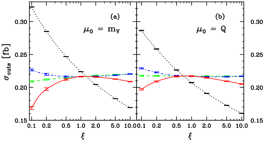
Figure 3: Dependence of the total $pp\,\mbox{$\rightarrow$}\,e^{+}\nu_{e}\,\mu^{+}\mu^{-}jj$ cross section at the LHC on the factorization and renormalization scales for two different choices of $\mu_{0}$. The NLO curves show $\sigma_{\rm cuts}^{\rm NLO}$ as a function of the scale parameter $\xi$ for three different cases: $\mu_{R}=\mu_{F}=\xi\mu_{0}$ (solid red), $\mu_{F}=\xi\mu_{0}$ and $\mu_{R}=\mu_{0}$ (dot-dashed blue), $\mu_{R}=\xi\mu_{0}$ and $\mu_{F}=\mu_{0}$ (dashed green). The LO cross sections depend only on $\mu_{F}$ (dotted black).

for different values of the renormalization and factorization scales, $\mu_{R}$ and $\mu_{F}$, which are taken as multiples of the mass scale $\mu_{0}$,

$$\mu_{R}=\xi_{R}\,\mu_{0}\;,\qquad\qquad\mu_{F}=\xi_{F}\,\mu_{0}\;.$$ (3.8)

In panel (a), $\mu_{0}$ is taken as the average vector boson mass involved in the reaction, $m_{V}=(m_{Z}+m_{W})/2$. In panel (b), $\mu_{0}=Q$, where $Q$ (see Eq. (2)) is the momentum transfer carried by the exchanged vector boson in VBF graphs as in Fig. 1(e), more precisely the vector boson attached to the upper (lower) quark line for QCD corrections and parton densities of the upper (lower) line. The LO cross section is of order $\alpha_{s}^{0}\alpha^{6}$ and therefore depends on the factorization scale only, which is set to $\mu_{F}=\xi\,\mu_{0}$ (dotted black curves). For $\sigma_{\rm cuts}^{\rm NLO}$ we show three cases: $\xi_{F}=\xi_{R}=\xi$ (solid red lines), $\xi_{F}=\xi,\xi_{R}=1$ (dot-dashed blue lines) and $\xi_{F}=1,\xi_{R}=\xi$ (dashed green lines). In the range $0.5\leq\xi\leq 2$ the variation of the NLO cross section amounts to only up to 2% in all cases for both choices of $\mu_{0}$. The scale dependence of the LO cross section over the entire range of $\xi$ is somewhat less pronounced for $\mu_{0}=Q$ than for $\mu_{0}=m_{V}$. The $K$ factors, $K=\sigma_{\rm NLO}/\sigma_{\rm LO}$, are given by $K=0.97$ for $\mu_{F}=\mu_{R}=m_{V}$ and $K=1.04$ for $\mu_{F}=\mu_{R}=Q$. These findings indicate that both choices, $\mu_{F}=m_{V}$ and $\mu_{F}=Q$, in $\sigma_{\rm cuts}^{\rm LO}$  yield a good estimate for the total cross section within typical VBF cuts. We will see below, however, that the NLO shape of some kinematical distributions can be approximated better by setting $\mu_{F}=Q$ in the corresponding LO predictions.

	$\sigma_{\rm cuts}^{\rm LO}$$(\mu_{0}=m_{V})$	$\sigma_{\rm cuts}^{\rm NLO}$$(\mu_{0}=m_{V})$	$\sigma_{\rm cuts}^{\rm LO}$$(\mu_{0}=Q)$	$\sigma_{\rm cuts}^{\rm NLO}$$(\mu_{0}=Q)$
$W^{+}Zjj$	$0.224$ fb	$0.217$ fb	$0.208$ fb	$0.217$ fb
$W^{-}Zjj$	$0.122$ fb	$0.120$ fb	$0.114$ fb	$0.120$ fb

Table 1: Total cross sections for $pp\mbox{$\rightarrow$}e^{+}\nu_{e}\,\mu^{+}\mu^{-}jj$ and $pp\mbox{$\rightarrow$}e^{-}\bar{\nu}_{e}\,\mu^{+}\mu^{-}jj$ via VBF at LO and NLO within the cuts of Eqs. (3.2)–(3.7) for the scale choices $\mu_{F}=\mu_{R}=m_{V}$ and $\mu_{F}=\mu_{R}=Q$. The statistical errors of the quoted results are at the permille level and therefore not given explicitly.

For reference, we list the values of $\sigma_{\rm cuts}$ at LO and NLO for $e^{+}\nu_{e}\,\mu^{+}\mu^{-}jj$ and $e^{-}\bar{\nu}_{e}\,\mu^{+}\mu^{-}jj$ production in VBF for the two scale choices, $\mu_{0}=m_{V}$ and $\mu_{0}=Q$ with $\xi_{R}=\xi_{F}=1$, in Tab. 1. In the following, we focus on $W^{+}Zjj$ production in VBF. The qualitative features of EW $W^{-}Zjj$ production are completely analogous.

Of particular importance for future LHC analyses are precise predictions for jet distributions and estimates of their residual theoretical uncertainties. In Fig. 4

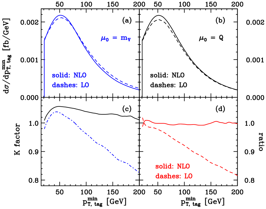
Figure 4: Transverse-momentum distribution of the tagging jet with the lowest $p_{T}$ in EW $e^{+}\nu_{e}\,\mu^{+}\mu^{-}jj$ production at the LHC for two different choices of $\mu_{0}$ [panels (a) and (b)]. Panel (c) shows the dynamical $K$ factors defined in Eq. (3.9) for $\mu_{0}=m_{V}$ (dot-dashed blue line) and $\mu_{0}=Q$ (solid black line). In panel (d) we have plotted the ratio $[d\sigma/dp_{T,{\rm tag}}^{\rm min}(\mu_{0}=m_{V})/[d\sigma/dp_{T,{\rm tag}}^{\rm min}(\mu_{0}=Q)]$ at LO (dashed red line) and NLO (solid red line).

we therefore present the transverse momentum distribution of the tagging jet with the lowest $p_{T}$ in EW $e^{+}\nu_{e}\,\mu^{+}\mu^{-}\,jj$ production for $\mu_{0}=m_{V}$ (a) and $\mu_{0}=Q$ (b) at LO and NLO (dashed and solid lines). Due to the cut (3.7) imposed on $M_{jj}$, contributions from events with low-$p_{T}$ tagging jets are suppressed and the peak of $d\sigma/dp_{T,{\rm tag}}^{\rm min}$ is located at about $p_{T}=50$ GeV. Therefore, increasing the $p_{Tj}$ cut of Eq. (3.2) to 30 or even 40 GeV would lead to only a modest decrease in the total cross section, an option which may be needed for high luminosity running. To emphasize the impact of NLO corrections, in panel (c) we show the dynamical $K$ factors, which are defined as

$$K(x)=\frac{d\sigma_{\rm NLO}/dx}{d\sigma_{\rm LO}/dx}\;$$ (3.9)

for the two scale choices discussed above. Panel (d) illustrates the LO and NLO ratios of the $p_{T}$ distributions for $\mu_{0}=m_{V}$ and $\mu_{0}=Q$,

$$\frac{d\sigma/dp_{T,{\rm tag}}^{\rm min}(\mu_{0}=m_{V})}{d\sigma/dp_{T,{\rm tag}}^{\rm min}(\mu_{0}=Q)}\;.$$ (3.10)

For a fixed scale $\mu_{0}=m_{V}$, the shape of the LO curve differs considerably from the NLO distribution, as indicated by a $K$ factor varying between $1.04$ and $0.8$. On the other hand, only a moderate change in shape results for a dynamical scale such as $\mu_{0}=Q$. The ratio of the $p_{T}$ distributions with the different scales reveals that the NLO result is barely sensitive to the choice of scale. However, setting $\mu_{F}=Q$ in the LO distributions appears to give a better estimate of the respective NLO results than the choice $\mu_{F}=m_{V}$. This feature is also present in NLO QCD calculations for deep inelastic scattering, which constitutes the dominant part of the VBF configurations.

The invariant-mass distribution of the tagging jet pair for $e^{+}\nu_{e}\,\mu^{+}\mu^{-}jj$ production is shown in Fig. 5

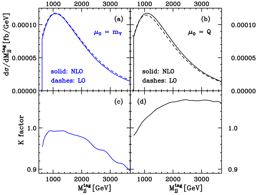
Figure 5: Invariant-mass distribution of the tagging jets in EW $e^{+}\nu_{e}\,\mu^{+}\mu^{-}jj$ production at the LHC for two different choices of $\mu_{0}$ [panels (a) and (b)]. Panels (c) and (d) show the dynamical $K$ factors defined in Eq. (3.9) for $\mu_{0}=m_{V}$ (blue line) and $\mu_{0}=Q$ (black line).

for $\mu_{0}=m_{V}$ and $\mu_{0}=Q$. Due to the $M_{jj}$ cut of Eq. (3.7) the cross section vanishes for $M_{jj}<600$ GeV. As for the $p_{T}$ distribution, very similar NLO results are obtained for the two scale choices, while the shapes of the LO curves differ somewhat. For the dynamical scale choice, $\mu_{0}=Q$, the LO result lies below the NLO curve, while in the case of a fixed scale, $\mu_{0}=m_{V}$, the LO curve exceeds the NLO prediction over the entire range of $M_{jj}$. The different effect of the two scales can be explained by the spectrum of $Q$ which ranges to values higher than $m_{V}$. Since the parton distribution functions $f(x,\mu_{F})$ in VBF-type reactions are probed at rather large $x$, in the process under investigation they decrease with increasing $\mu_{F}$ and are therefore smaller for typical values of $Q$ than for $m_{V}$. At NLO, this decrease is counterbalanced by respective contributions in the partonic cross sections and the theoretical uncertainty associated with the choice of factorization scale is reduced.

Figure 6

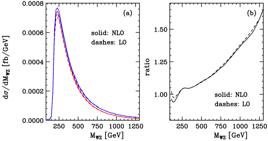
Figure 6: Panel (a) shows the LO (dashed) and NLO (solid) distributions of the four-lepton invariant-mass in EW $e^{+}\nu_{e}\,\mu^{+}\mu^{-}jj$ production at the LHC for Higgs masses of $m_{H}=120$ GeV (red lower lines) and $m_{H}=10$ TeV (blue upper lines). In panel (b), the ratio of the distributions for the different Higgs masses is displayed for the LO and the NLO results. The factorization and renormalization scales are taken as $\mu_{F}=\mu_{R}=Q$.

shows the four lepton invariant mass distribution in EW $e^{+}\nu_{e}\,\mu^{+}\mu^{-}jj$ production with $M_{WZ}$ being defined as

$$M_{WZ}=\sqrt{(p_{e^{+}}+p_{\nu_{e}}+p_{\mu^{+}}+p_{\mu^{-}})^{2}}$$ (3.11)

for two different values of the Higgs boson mass, $m_{H}=120$ GeV and $m_{H}=10$ TeV. For the latter choice, contributions from Higgs boson exchange diagrams are effectively eliminated, i.e. results correspond to a “Higgsless model”. Since in $W^{\pm}Zjj$ production processes the Higgs boson does not appear in the $s$-channel but only as a $t$-channel exchange boson, no pronounced resonance behavior as, for example, in the $ZZjj$ channel, is expected. Panel (a) shows that, indeed, similar shapes are obtained for both choices of $m_{H}$. The ratio of the two distributions,

$$\frac{d\sigma/dM_{WZ}(m_{H}=10~{}\mathrm{TeV})}{d\sigma/dM_{WZ}(m_{H}=120~{}\mathrm{GeV})}\;,$$ (3.12)

displayed in panel (b), reveals, however, a rise in the cross section for large $M_{WZ}$, if the Higgs boson becomes very heavy.

4 Conclusions

In this article we have described the calculation of the NLO QCD corrections to EW $e^{+}\nu_{e}\,\mu^{+}\mu^{-}jj$ and $e^{-}\bar{\nu}_{e}\,\mu^{+}\mu^{-}jj$ production at the LHC, and their implementation in a fully flexible parton-level Monte Carlo program that allows for the computation of kinematic distributions within realistic experimental cuts. We found that the scale uncertainties of the NLO predictions for total cross sections are at the 2% level, which indicates that the perturbative calculation is under excellent control. Care has to be taken, however, if NLO distributions are to be approximated by LO results, as shapes can change considerably when going from LO to NLO. In this regard, a “proper” choice of factorization scale can help. We found that, with a factorization scale chosen as the momentum transfer, $Q$, of the $t$-channel electroweak boson, the LO calculation can better reproduce the shape of NLO distributions than when taking a fixed scale, $\mu_{F}=m_{V}$.

References

- [1] ATLAS Collaboration, ATLAS TDR, Report No. CERN/LHCC/99-15 (1999); E. Richter-Was and M. Sapinski, Acta Phys. Pol. B 30, 1001 (1999); B. P. Kersevan and E. Richter-Was, Eur. Phys. J. C 25, 379 (2002) [arXiv:hep-ph/0203148].
- [2] G. L. Bayatian et al., CMS TDR, Report No. CERN/LHCC/2006-021 (2006); R. Kinnunen and D. Denegri, CMS Note No. 1997/057; R. Kinnunen and A. Nikitenko, Report No. CMS TN/97-106; R. Kinnunen and D. Denegri, arXiv:hep-ph/9907291.
- [3] D. L. Rainwater, PhD thesis, arXiv:hep-ph/9908378; D. Rainwater and D. Zeppenfeld, Phys. Rev. D 60, 113004 (1999) [Erratum-ibid. D 61, 099901 (2000)] [arXiv:hep-ph/9906218]; N. Kauer, T. Plehn, D. Rainwater, and D. Zeppenfeld, Phys. Lett. B 503, 113 (2001) [arXiv:hep-ph/0012351].
- [4] T. Plehn, D. Rainwater, and D. Zeppenfeld, Phys. Rev. Lett. 88, 051801 (2002); V. Hankele, G. Klämke, D. Zeppenfeld, arXiv:hep-ph/0605117; V. Hankele, G. Klämke, D. Zeppenfeld, and T. Figy, Phys. Rev. D 74, 095001 (2006) [arXiv: hep-ph/0609075].
- [5] D. Zeppenfeld, R. Kinnunen, A. Nikitenko, and E. Richter-Was, Phys. Rev. D 62, 013009 (2000) [arXiv:hep-ph/0002036]; D. Zeppenfeld, in Proc. of the APS/DPF/DPB Summer Study on the Future of Particle Physics, Snowmass, 2001 edited by N. Graf, eConf C010630, p. 123 (2001) [arXiv:hep-ph/0203123]; A. Belyaev and L. Reina, JHEP 0208, 041 (2002) [arXiv:hep-ph/0205270]; M. Dührssen et al., Phys. Rev. D 70, 113009 (2004) [arXiv:hep-ph/0406323].
- [6] Some recent work and reviews can be found in : O. J. P. Eboli, M. C. Gonzalez-Garcia, and J. K. Mizukoshi, Phys. Rev. D 74, 073005 (2006) [arXiv:hep-ph/0606118]; T. L. Barklow et al., arXiv:hep-ph/9704217; M. S. Chanowitz, Czech. J. Phys. 55, B45 (2005) [arXiv:hep-ph/0412203] and references therein.
- [7] B. Jäger, C. Oleari, and D. Zeppenfeld, JHEP 0607, 015 (2006) [arXiv:hep-ph/0603177].
- [8] B. Jäger, C. Oleari, and D. Zeppenfeld, Phys. Rev. D 73 113006 (2006) [arXiv:hep-ph/0604200]; B. Jäger, C. Oleari, and D. Zeppenfeld, arXiv:hep-ph/0608272.
- [9] A. Dobado, M. J. Herrero, and J. Terron, Z. Phys. C 50, 465 (1991).
- [10] R. N. Cahn and S. Dawson, Phys. Lett. B 136, 196 (1984) [Erratum-ibid. B 138, 464 (1984)]; S. Dawson, Nucl. Phys. B249, 42 (1985); M. J. Duncan, G. L. Kane, and W. W. Repko, Nucl. Phys. B272, 517 (1986).
- [11] V. D. Barger, K. Cheung, T. Han, A. Stange, and D. Zeppenfeld, Phys. Rev. D 46 2028 (1992).
- [12] J. Bagger et al., Phys. Rev. D 49, 1246 (1994) [arXiv:hep-ph/9306256]; J. Bagger et al., Phys. Rev. D 52, 3878 (1995) [arXiv:hep-ph/9504426].
- [13] K. Hagiwara and D. Zeppenfeld, Nucl. Phys. B274, 1 (1986); K. Hagiwara and D. Zeppenfeld, Nucl. Phys. B313, 560 (1989).
- [14] C. Georg, Diploma thesis, Universität Karlsruhe (2005), http://www-itp.physik.uni-karlsruhe.de/diplomatheses.de.shtml.
- [15] S. Catani and M. H. Seymour, Nucl. Phys. B485, 291 (1997) [Erratum-ibid. B510, 503 (1997)] [arXiv:hep-ph/9605323].
- [16] T. Figy, C. Oleari, and D. Zeppenfeld, Phys. Rev. D 68, 073005 (2003) [arXiv:hep-ph/0306109].
- [17] Warren Siegel, Phys. Lett. B 84, 193 (1979); Warren Siegel, Phys. Lett. B 94, 37 (1980).
- [18] G. Passarino and M. J. Veltman, Nucl. Phys. B160, 151 (1979).
- [19] A. Denner and S. Dittmaier, Nucl. Phys. B658, 175 (2003) [arXiv:hep-ph/0212259]; Nucl. Phys. B734, 62 (2006) [arXiv:hep-ph/0509141].
- [20] T. Stelzer and W. F. Long, Comput. Phys. Commun. 81, 357 (1994) [arXiv:hep-ph/9401258]; F. Maltoni and T. Stelzer, JHEP 0302, 027 (2003) [arXiv:hep-ph/0208156].
- [21] C. Oleari and D. Zeppenfeld, Phys. Rev. D 69, 093004 (2004) [arXiv:hep-ph/0310156].
- [22] P. Konar and D. Zeppenfeld, arXiv:hep-ph/0612119.
- [23] J. Pumplin, D. R. Stump, J. Huston, H. L. Lai, P. Nadolsky, and W. K. Tung, JHEP 0207, 012 (2002) [arXiv:hep-ph/0201195].
- [24] A. Denner, S. Dittmaier, M. Roth, and D. Wackeroth, Nucl. Phys. B560, 33 (1999) [arXiv:hep-ph/9904472].
- [25] S. Catani, Yu. L. Dokshitzer, and B. R. Webber, Phys. Lett. B 285 291 (1992); S. Catani, Yu. L. Dokshitzer, M. H. Seymour, and B. R. Webber, Nucl. Phys. B406 187 (1993); S. D. Ellis and D. E. Soper, Phys. Rev. D 48 3160 (1993).
- [26] G. C. Blazey et al., arXiv:hep-ex/0005012.