Abstract

We reconsider thermal production of gravitinos in the early universe, adding to previously considered $2\to 2$ gauge scatterings: a) production via $1\to 2$ decays, allowed by thermal masses: this is the main new effect; b) the effect of the top Yukawa coupling; c) a proper treatment of the reheating process. Our final result behaves physically (larger couplings give a larger rate) and is twice larger than previous results, implying e.g. a twice stronger constraint on the reheating temperature. Accessory results about (supersymmetric) theories at finite temperature and gravitino couplings might have some interest.

1 Introduction

We compute the abundance of gravitinos thermally produced in the early universe at temperature $T$. In the usual scenario where sparticles around the weak scale keep it naturally small, this process implies an important constraint on the maximal reheating temperature, possibly saturated if such gravitinos are all observed Dark Matter (DM). If instead sparticles exist much above the weak scale, gravitino production is one of their very few experimental implications that survive.

The gravitino production thermal rate was previously computed in [gravitinoCosmo, Buch] at leading order in the gauge couplings $g_{3}$ (and $g_{2},g_{Y}$ in [postBuch]; we will add effects due the top Yukawa coupling, which also has a sizeable value). This roughly amounts to compute $2\to 2$ scatterings (like gluon + gluon $\to$ gluon $\to$ gluino + gravitino), with thermal effects ignored everywhere expect in the propagator of the virtual intermediate gluon: a massless gluon exchanged in the $t$-channel gives an infinite cross-section because it mediates a long-range Coulomb-like force; the resulting logarithmic divergence is cut off by the thermal mass of the gluon, $m\sim gT$, leaving a $\ln T/m$. The explicit expression for the number of scatterings per space-time volume, at leading order in the dominant QCD gauge coupling, was found to be [Buch, postBuch]

$$\gamma_{\rm scattering}=\frac{T^{6}}{2\pi^{3}\bar{M}_{\rm Pl}^{2}}\left(1+\frac{M_{3}^{2}}{3m_{3/2}^{2}}\right)f(g_{3}),\qquad f(g_{3})=\frac{320.}{\pi^{2}}g_{3}^{2}\ln\frac{1.2}{g_{3}}$$ (1.1)

where $\bar{M}_{\rm Pl}=2.4~{}10^{18}\,{\rm GeV}$ is the reduced Planck mass, $M_{3}$ is gluino mass and $m_{3/2}$ is the gravitino mass. This production rate unphysically decreases for $g_{3}\,\raise 1.29167pt\hbox{$>$\kern-7.5pt\lower 4.30554pt\hbox{$\sim$}}\,0.7$ becoming negative for $g_{3}\,\raise 1.29167pt\hbox{$>$\kern-7.5pt\lower 4.30554pt\hbox{$\sim$}}\,1.2$. Fig. 1 shows that the physical value, $g_{3}\approx 0.85$ at $T\sim 10^{10}\,{\rm GeV}$, lies in the region where the leading-order rate function $f(g_{3})$ (dashed line) is unreliable. Fig. 1 also illustrates our final result (to be precisely described in section 4.2): $f$ will be replaced by the continuous lines, which agree with the leading order result at $g\sim m/T\ll 1$ and differ at $g\sim 1$.

Let us now explain why the leading-order approximation in (1.1) starts to be inadequate already at $g\sim 0.7$. In thermal field theory higher order corrections are usually suppressed by $g/\pi$: somewhat worse than the usual expansion coefficient $(g/\pi)^{2}$ at $T=0$, but still typically good enough at $g\sim 0.7$. Naïve power counting fails (without signaling a breaking of the perturbative expansion) when some new phenomenon only starts entering at higher orders, and this is what happens in the case of gravitino production: a new simpler process gives corrections of relative order $(g\pi)^{2}$. The gravitino couples to two particles with different thermal masses: gluon/gluino, and quark/squark. Since thermal masses grow like $T$, this gives rise to a new process with a rate growing like $T^{6}$: gravitino production via decays, such as gluon $\to$ gluino + gravitino, whose rate can be crudely estimated as

$$\gamma_{\rm decay}\sim\frac{m}{T}\frac{T^{3}\Gamma}{\pi^{2}}\sim\frac{m^{4}T^{2}}{\pi^{3}\bar{M}_{\rm Pl}^{2}}\sim\frac{g^{4}}{\pi^{3}}\frac{T^{6}}{\bar{M}_{\rm Pl}^{2}}$$ (1.2)

Indeed $\gamma_{\rm decay}$ is of course proportional to the decay rate at rest $\Gamma\sim m^{3}/\pi\bar{M}^{2}_{\rm Pl}$; which is slowed down by the Lorentz dilatation $m/T$ factor; the $T^{3}$ takes care of dimensions, and less $\pi$ are present at the denominator because a $1\to 2$ decay involves less particles than a $2\to 2$ scattering. So, despite being higher order in $g$, the decay rate can be enhanced by a phase space factor $\pi^{2}$. Subsequent higher order corrections should be suppressed by the usual $g/\pi$ factors. Our goal is including such enhanced higher order terms, and this finite-temperature computation is practically feasible because a decay is a simple enough process.

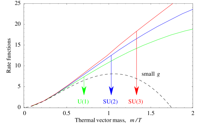
Figure 1: Functions $f_{3}$, $f_{2}$ and $f_{1}$ that, as summarized in section 4.2, describe our result for the gravitino production rate from ${\rm SU}(3)_{c}$ (upper continuous curve, in red), ${\rm SU}(2)_{L}$ (middle continuous curve, in blue), ${\rm U}(1)_{Y}$ (lower continuous curve, in green) gauge interactions. The arrows indicate the MSSM values of the thermal mass at $T\sim 10^{9}\,{\rm GeV}$. The lower dashed curve shows the result from [Buch], which agrees with our result in the limit of small gauge coupling, and behaves unphysically for relevant ${\cal O}(1)$ values of the MSSM gauge couplings.

So far we explained the physical picture in a simple intuitive way. A more precise technical language is necessary to present how we will proceed. To get the gravitino production rate we actually compute the imaginary part of the gravitino propagator in the thermal plasma. Thermal effects distort the dispersion relations $E(k)$ of gluons, gluinos, quarks, squarks by i) adding a thermal mass $E^{2}=k^{2}+m^{2}(k)$ to the modes already existing at zero temperature; ii) by introducing new collective excitations (gluons with longitudinal polarization, gluinos with ‘wrong’ helicity, …) with their own dispersion relation; iii) beyond the two poles mentioned above, the spectral densities of particles in a thermal plasma also develop a ‘continuum’ contribution, that can be thought of as a parton-like distribution, with a continuum range of masses. Physically it arises because particles can exchange energy with the plasma.

In previous works [Buch, postBuch] the gluon thermal mass was taken into account to regulate infra-red divergences encountered in scattering rates, and the contribution of the gluon ‘continuum’ was computed using a standard technique introduced in axion computations [BY], that allows to extract the rate at leading order in $g$. This was achieved by introducing an arbitrary splitting scale $k$ that obeys $gT\ll k\ll T$.

We will not use this technique: because its validity is doubtful for $g_{3}\approx 0.85$, and because we actually want to include the enhanced higher order terms, taking into account that a gravitino (unlike an axion) couples to two particles with different thermal masses. We will instead compute the decay diagram (D in fig. 3) using resummed finite-temperature propagators for gluons, gluinos, quarks, squarks. The perturbative expansion of this diagram D contains the two-loop diagrams in fig. 3: their imaginary parts correspond to well-defined combinations of scattering processes, as dictated by cutting rules. This fixes how scatterings must be subtracted in order to avoid overcountings of effects already described by thermal masses via diagram D. In section 2 we compute the subtracted scattering rates, in section 4 we compute the gravitino production rate via ‘decay’, and in section 5 we add the rate due to the top quark Yukawa coupling.

In section 6 we sum these effects and compute the gravitino abundance writing a set of Boltzmann equations that describe the reheating process, previously approximated assuming a maximal temperature equal to the reheating temperature $T_{\rm RH}$. Our results are summarized in the conclusions, section 7.

In the passing we address some issues related to finite-temperature and to supersymmetry. In section 3 we list explicit values for thermal masses for all particles and sparticles, noticing that they obey some supersymmetric relation. Appendix A gives a (non uselessly) fully precise summary of gravitino interactions, and in appendices B, LABEL:thermalF we collect full expressions for the thermal corrections to vector and fermion propagators.

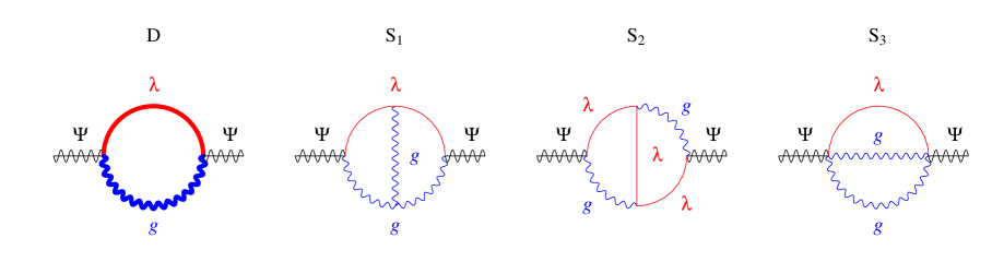
Figure 2: Some Feynman diagrams that contribute to the imaginary part of the gravitino propagator. Thick lines denote resummed thermal propagators for the gluon $g$ and gluino $\lambda$. We do not plot diagrams involving quarks $q$ and squarks $\tilde{q}$, but they are of course included in our computation.

Figure 3: Two-loop Feynman diagrams that appear in the expansion of diagram ${\rm D}$, that resums all higher loop diagrams with iterated one-loop corrections to gluon and gluino propagators.

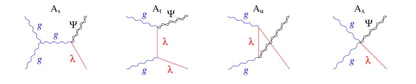
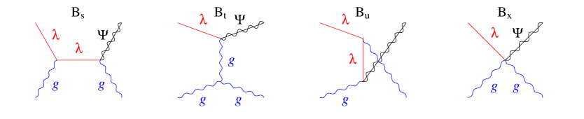
Figure 4: Feynman diagrams that contribute to $gg\to\lambda\Psi$ scatterings.

Figure 5: Feynman diagrams that contribute to $g\lambda\to g\Psi$ scatterings.

2 Subtracted scattering rate

Gravitinos $\Psi_{\mu}$ with momentum $P=(E,\mbox{\normalsize\boldmath$p$})$ are produced via their coupling $\bar{\Psi}_{\mu}S^{\mu}/{2\bar{M}_{\mathrm{Pl}}}$, where $S^{\mu}$ is the supercurrent of the visible sector of a supersymmetric theory, here assumed to be the MSSM. The visible sector is thermalized, while the gravitino is not, since its coupling to the MSSM plasma is weak. According to the general formalism of thermal field theory [LeBellac], the production rate of such a weakly interacting fermion is related to the imaginary part of its propagator $\Pi$ as

$$\gamma=\frac{dN}{dV\,dt}=-2\int d\vec{P}\,f_{F}(E)\mathop{\rm Im}\Pi=\int d\vec{P}~{}\Pi^{<}(P),\qquad d\vec{P}\equiv\frac{d^{3}p}{2E(2\pi)^{3}}.$$ (2.1)

Here $\Pi^{<}$ is the non time-ordered gravitino propagator summed over its polarizations i.e. traced with the gravitino polarization tensor $\Pi_{\mu\nu}$ (appendix A gives explicit expressions):

$$\Pi^{<}(P)=\frac{1}{4\bar{M}_{\mathrm{Pl}}^{2}}\mathop{\rm Tr}\big{[}\Pi_{\mu\nu}(P)\langle S^{\nu}(P){\bar{S}}^{\mu}(-P)\rangle_{T}\big{]}$$ (2.2)

where $\langle\cdots\rangle_{T}$ denotes thermal average. We employ $\Pi^{<}$ because it gives slightly cleaner formulæ than $\mathop{\rm Im}\Pi$. Eq. (2.1) is valid at leading order in the gravitino coupling $\bar{M}_{\mathrm{Pl}}^{-1}$, and to all orders in the MSSM couplings, $g_{Y,2,3}$ and $\lambda_{t}$. Extracting predictions from (2.1) is limited only by our ability to evaluate (2.2).

Thermal field theory cutting rules allow to see that, at leading order in the MSSM couplings, eq. (2.1) is equivalent to summing rates for the various tree-level processes that lead to gravitino production. At tree level this formalism is more cumbersome than a direct computation of production rates. However, in this paper we want to take into account finite temperature corrections to the MSSM particle propagators arising at one loop level: eq. (2.1) becomes more convenient because it cleanly dictates how one must resolve ambiguities encountered in scattering computations that arise because Lorentz invariance is broken by the thermal plasma.

Fig. 3 shows some main Feynman diagrams that contribute to $\mathop{\rm Im}\Pi$. What we actually compute in this paper is the first one-loop diagram ‘D’, using the Feynman gauge resummed finite-temperature propagators for the gluon and gluino in the loop. Therefore it describes a sum of an infinite number of multi-loop diagrams: the lowest-order ones are shown in fig. 3. Resummation is needed because thermal effect drastically change the gluon and gluino propagators, in particular opening a phase space for decays, such as $g\rightarrow\lambda\Psi$ and/or $\lambda\rightarrow g\Psi$. Clearly diagram D contains this decay process. However, by cutting fig. 3, one sees that diagram D also describes some of the $2\rightarrow 2$ scattering processes computed in previous analyses [Buch]. Therefore, before starting the computation, we clarify this issue showing how the total gravitino production rate is obtained.

The total scattering rate is the sum of various $2\to 2$ processes A, B, C,…, listed in table 1. Each process is the modulus squared of the sum of a few amplitudes, corresponding to the single Feynman diagrams, that we label as $s,t,u,x$:

$$\gamma_{\mathrm{scattering}}=|A_{s}+A_{t}+A_{u}+A_{x}|^{2}+|B_{s}+B_{t}+B_{u}+B_{x}|^{2}+\cdots.$$

This notation indicates that often 4 diagrams contribute to a given process: 3 diagrams are generated by $s$, $t$ and $u$-channel exchange of some particle among two vertices ($g_{3}$ and $1/M_{\mathrm{Pl}}$), and a fourth diagram arises from a quartic supergravity vertex with coupling $g/M_{\mathrm{Pl}}$. Fig. 5 and 5 show concrete examples of the 4 diagrams that contribute to $gg\to\Psi\lambda$ and to $g\lambda\to\Psi g$ scatterings, respectively. The latter rate is logarithmically infra-red (IR) divergent, because diagram B${}_{t}$ is mediated by $t$-channel gluon exchange, that describes a Coulomb-like scattering.

The main result can be obtained by careful visual inspection of cutting rules: diagram D describes the sum $|A_{s}|^{2}+|A_{t}|^{2}+|A_{u}|^{2}+|B_{s}|^{2}+|B_{t}|^{2}+|B_{u}|^{2}+\cdots$ of the modulus squared of all $2\to 2$ diagrams that contain the gauge coupling $g_{3}$. $2\to 2$ scattering rates generated by supergravity quartic vertices are instead described by diagrams like S${}_{3}$ in fig. 3. Some cuts of the two loop diagrams like S${}_{1}$ and S${}_{2}$ describe the interference terms among the various Feynman diagrams. (Notice that the imaginary part of a single two-loop diagram can describe contributions to different scattering processes). Other cuts of these diagrams describe one loop corrections to the gravitino vertices, that do not give any leading order contribution if thermal masses are neglected. Thermal masses open a phase space for $1\to 2$ processes (we can neglect the decay rate generated by zero-temperature masses $m$, since we are interested in $T\gg m$), and we will later argue that we can still neglect thermal corrections to the gravitino vertex.

	process		$|\mathscr{A}|^{2}_{\mathrm{full}}$	$|\mathscr{A}|^{2}_{\mathrm{subtracted}}$
F	$\lambda\lambda$ $\to$	$\lambda\Psi$	$-8C{(s^{2}+t^{2}+u^{2})^{2}}/{stu}$	0
A	$gg$ $\to$	$\lambda\Psi$	$\phantom{+}4C(s+2t+2t^{2}/s)$	$-2sC$
B	$g\lambda$ $\to$	$g\Psi$	$-4C(t+2s+2s^{2}/t)$	$\phantom{+}2tC$
H	$\tilde{q}\lambda$ $\to$	$\tilde{q}\Psi$	$-2C^{\prime}(t+2s+2{s^{2}}/{t})$	$-tC^{\prime}$
J	$\tilde{q}\bar{\tilde{q}}$ $\to$	$\lambda\Psi$	$\phantom{+}2C^{\prime}(s+2t+2{t^{2}}/{s})$	$\phantom{+}sC^{\prime}$
C	$\tilde{q}g$ $\to$	$q\Psi$	$\phantom{+}2sC^{\prime}$	0
D	$gq$ $\to$	$\tilde{q}\Psi$	$-2tC^{\prime}$	0
E	$\bar{\tilde{q}}q$ $\to$	$g\Psi$	$-2tC^{\prime}$	0
G	$q\lambda$ $\to$	$q\Psi$	$-4C^{\prime}(s+{s^{2}}/{t})$	0
I	$q\bar{q}$ $\to$	$\lambda\Psi$	$-4C^{\prime}(t+{t^{2}}/{s})$	0

Table 1: Squared matrix elements for gravitino ($\Psi$) production in units of $g^{2}_{N}/\bar{M}^{2}_{\mathrm{Pl}}(1+M^{2}_{N}/3m_{3/2}^{2})$, summed over all polarizations and gauge indices. The result hold for all three factors of the SM gauge group with $N=\{1,2,3\}$, although the notations are appropriate for the ${\rm SU}(3)$ case: $g,\lambda,q,\tilde{q}$ denote gluons, gluinos, quarks, squarks. The gauge factors $C_{N}$ and $C^{\prime}_{N}$ are defined in the text. Rates A and B are the sum of vector and ghost contributions.

In conclusion, the total gravitino production rate due to gauge couplings will be computed as

$$\gamma=\gamma_{D}+\gamma_{S}^{\mathrm{sub}},$$ (2.3)

the sum of diagram D (that describes decay plus modulus squared of many single $2\rightarrow 2$ diagrams) plus the set of remaining $2\rightarrow 2$ rates, obtained by subtracting from the total scattering rate $\gamma_{S}$ the effects already included in $\gamma_{D}$. Explicit results for $\gamma_{D}$ and for $\gamma_{S}^{\rm sub}$ will be given in eq. (4.6) and eq. (2.6) respectively, and the conclusions will describe how to use them.

Before proceeding to actual computations, we have to clarify the issues of gravitino coupling and gravitino gauge invariance. We are interested in $T\gg m$, where $m$ denotes sparticle or gravitino masses: gravitino $\leftrightarrow$ Goldstino equivalence (appendix A) means that at leading order in $m/T$ the massive gravitino field $\Psi_{\mu}$ can be replaced with two massless field: a massless gravitino $\psi$ coupled to the supercurrent $S_{\mu}$ (given in eq. (A.28), it can be evaluated in the supersymmetric limit ignoring soft terms) plus a massless Goldstino $\chi$, coupled to the divergence of the supercurrent (given in eq. (A.29), only the soft terms factored out are relevant):

$$\mathscr{L}_{\mathrm{int}}=\frac{\bar{\psi}_{\mu}S^{\mu}}{2\bar{M}_{\text{Pl}}}+\frac{\bar{\chi}\,(\partial_{\mu}S^{\mu})}{\sqrt{6}\bar{M}_{\mathrm{Pl}}m_{3/2}}\ .$$ (2.4)

The gravitino production rate is given by $\gamma(\Psi_{\mu})\simeq\gamma(\psi_{\mu})+\gamma(\chi)$. While the total rate is gauge independent (vectors have ${\rm SU}(3)_{c}\otimes{\rm SU}(2)_{L}\otimes\mathrm{U}(1)_{Y}$ gauge invariance; the computation of $\gamma(\psi_{\mu})$ also involves gravitino gauge invariance), its splitting in resummed and not-resummed contributions is not. We are resumming a well-defined class of effects, but we cannot systematically include all the effects up to a given order in $g$: therefore our result has a residual gauge-dependence, of relative order $g^{2}/\pi^{2}$, due to partial inclusion of higher-order terms. To make the computation feasible, we choose for vectors the Feynman gauge, and for the massless gravitino $\psi_{\mu}$ the gauge where its propagator and polarization tensor does not involve terms containing $P_{\mu}$ or $P_{\nu}$, eq. (A.23):

$$\Pi_{\mu\nu}^{3/2}=-\frac{1}{2}\gamma_{\mu}P/\,\gamma_{\nu}-P/\,\eta_{\mu\nu}.$$ (2.5)

One first motivation for this choice is that, in the supersymmetric limit, the full supercurrent satisfies $P_{\mu}S^{\mu}=0$, while sub-sets of $S_{\mu}$ are not separately conserved: with choice (2.5) we never have to deal with such terms. Of course, the same gauge is used for computing both the resummed diagram D and the subtracted scattering rates.

Table 1 gives explicit values for the subtracted massless gravitino and Goldstino scattering rates due to gauge interactions. It is important to notice that, unlike the total rate, the subtracted rates are infra-red convergent: no $1/t$ factors appear because all divergent Coloumb-like scatterings, like $|B_{t}|^{2}$, are included in diagram D, that we compute using thermal masses that provide the physical cut-off. Unlike in the conventional technique [BY] employed in [Buch, postBuch], our technique does not need to introduce an arbitrary splitting scale $k_{\ast}$ that satisfies the problematic conditions $gT\ll k_{\ast}\ll T$ in order to control infra-red divergences. Some contributions to subtracted scattering rates turn out to be negative, but the total rate will be positive and dominated by diagram D. In Feynman gauge, rates for the processes A and B (the ones that involve two vectors) actually are the sum of scatterings involving two vectors (four diagrams, computed with the Feynman polarization tensor $\sum\epsilon_{\mu}\epsilon_{\nu}^{\ast}=-\eta_{\mu\nu}$) plus scatterings containing two ghosts (one diagram, negative $|\mathscr{A}|^{2}$).

A curious fact happens. Despite the fact that the massless gravitino $\psi$ and the Goldstino $\chi$ have different couplings (in particular the Goldstino has no coupling to quark/squark, and consequently a reduced set of Feynman diagrams), the differential production cross sections for these two particles are the same, process by process, up to the universal factor $M_{N}^{2}/3m_{3/2}^{2}$, where $M_{1,2,3}$ are the gaugino masses. We don’t know if there is a simple generic reason behind this equality. The second reason for choosing the gravitino projector of eq. (2.5) is that it respects this equality also for subtracted scattering rates.

Subtracted rates for processes C, D, E, G, I vanish, and looking at Goldstinos one can easily understand why: a single Goldstino diagram contributes, such that no interference terms exist. This is not the case for scatterings H and J, where a second Goldstino diagram contributes, generated by the quartic Goldstino coupling in eq. (A.29). (This extra coupling is not present for the ghost scatterings in A and B analogous to H and J, as we employ a non-supersymmetric gauge without ghostinos). In case of scattering F the subtracted rate vanishes because proportional to $s+t+u=0$. A $1/2!$ factor must be included for the A and F processes that have equal initial state particles, and a factor 2 for C, D, G, H that can occur with particles and with anti-particles. The total result for the subtracted gravitino production rate is

$$\gamma_{S}^{\mathrm{sub}}=1.29\frac{T^{6}}{8\pi^{5}\bar{M}_{\mathrm{Pl}}^{2}}\sum_{N=1}^{3}g_{N}^{2}(1+\frac{M_{N}^{2}}{3m_{3/2}^{2}})(C_{N}^{\prime}-C_{N})$$ (2.6)

where the numerical factor accounts for the difference with respect to the scattering rate computed in Boltzmann approximation, where $\gamma\approx\sigma T^{6}/\pi^{4}$ where $\sigma=\sum\int_{-s}^{0}dt~{}|\mathscr{A}|^{2}/16\pi s^{2}$ is a constant. The sum runs over the three components $\mathrm{U}(1)_{Y}\otimes{\rm SU}(2)_{L}\otimes{\rm SU}(3)_{c}$ of the MSSM gauge group with $N=\{1,2,3\}$, and $C_{N}=|f^{abc}|^{2}=N(N^{2}-1)=\{0,6,24\}$ and $C_{N}^{\prime}=\sum_{\Phi}|T_{ij}^{a}|^{2}=\{11,21,48\}$ where $\sum_{\Phi}$ runs over all chiral multiplets. We use the standard normalization for hypercharge, where left-handed leptons have $Y=-1/2$, that differs from the SU(5) normalization by a factor $\sqrt{3/5}$. All parameters are renormalized at an energy scale $\mu\sim T$.

The next step is computing diagram D: we first need to introduce finite temperature effects.

3 Finite temperature effects

We here summarize some well known results from quantum field theory at finite temperature that are relevant for our computations: the spectral densities of scalars, fermions and vectors that play a rôle analogous to parton densities in hadron scattering processes. This section also contains a few original points: practical formulæ for thermal masses that apply to generic supersymmetric models, the observation that thermal effects respect supersymmetry at $E\gg T$; we explain what qualitatively changes and why we must go beyond the Hard Thermal Loop approximation; we discuss a possibly non-standard point of view about the problem of negative spectral densities.

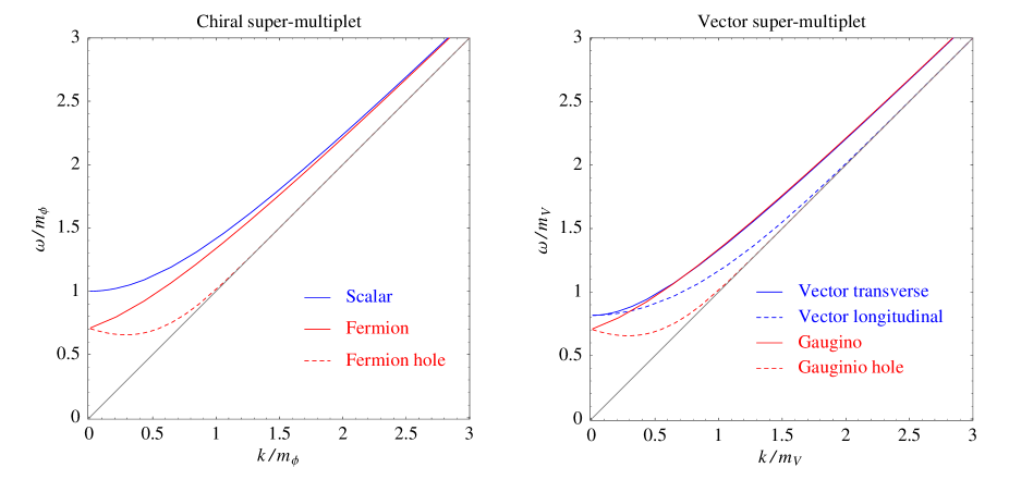
Figure 6: Dispersion relations at finite temperature in HTL approximation for the components within a chiral (left) and vector (right) massless super-multiplet. Thermal effects are supersymmetric at $k\gg m\sim gT$.

3.1 The Hard Thermal Loop approximation

Thermal corrections simplify when one restricts the attention to diagrams with ‘soft’ external momenta, $k\ll T$ [Pisarski92, LeBellac]. This approximation is useful if couplings are small, $g\ll 1$, as it describes collective phenomena that develop at energies of ${\cal O}(gT)$ via simple effective thermal Lagrangians. In the rest frame of the plasma, the non-local HTL Lagrangian for scalars $\phi$, fermions $\psi$ and vectors is [Pisarski92, LeBellac]

$$\mathscr{L}_{\rm HTL}=m_{S}^{2}|A|^{2}+m_{F}^{2}\int_{\Omega}\bar{\psi}\frac{i\hat{K}/}{\hat{K}\cdot D}\psi-m_{V}^{2}{\rm Tr}\int_{\Omega}F_{\mu\alpha}\frac{\hat{K}_{\alpha}\hat{K}_{\beta}}{(\hat{K}\cdot D)^{2}}F_{\beta\mu}+\cdots$$ (3.1)

where $\cdots$ denotes Yukawa or scalar couplings that do not receive HTL corrections; gauge couplings receive thermal corrections such that $\mathscr{L}_{\rm HTL}$ is gauge invariant (indeed $D$ denotes the usual gauge-covariant derivative); $\hat{K}=(1,\hat{\mbox{\normalsize\boldmath$k$}})$ is the ‘loop’ momentum ($\hat{K}^{2}=0$); $\int_{\Omega}=\int d\Omega/4\pi$ denotes angular average. It is performed analytically in the more explicit results in appendices B and LABEL:thermalF

The key parameters are ‘thermal masses’ of order $m\sim gT$. By explicit computation we find the following values for thermal masses in an unbroken supersymmetric theory with massless chiral $\Phi=(\phi,\xi)$ and vector $V=(V_{\mu},\lambda)$ superfields:

$$m_{\phi}^{2}=2{m_{\xi}^{2}}=\bigg{[}\frac{C_{R}}{2}g^{2}+\frac{1}{4}\lambda^{2}\bigg{]}T^{2},\qquad m_{V}^{2}=2m_{\lambda}^{2}=\bigg{[}g^{2}\frac{C_{V}+T^{2}_{R}}{4}\bigg{]}T^{2}$$ (3.2)

where $g$ is the gauge coupling and $\lambda$ the coupling in the superpotential $W=\lambda\Phi\Phi^{\prime}\Phi^{\prime\prime}$. Summation over gauge, flavor and any indices is understood. The group factors $C_{R}$ and $T^{2}_{R}$ are defined as ${\rm Tr}T_{R}^{a}T_{R}^{b}=T_{R}^{2}\delta^{ab}$ (index of the representation) and as $(T_{R}^{a}T_{R}^{a})_{ij}=C_{R}\delta_{ij}$ (quadratic Casimir) where the generators are in the representation $R$. By summing both over $ij$ and over $ab$ one finds that they are related by $T^{2}_{R}\dim G=C_{R}\dim R$. Explicit values are $T_{R}^{2}=1/2$ and $C_{R}=(N^{2}-1)/2N$ for the fundamental of SU($N$) ($\dim R=N$, $\dim G=N^{2}-1$), $C_{V}=N$ for the adjoint of SU($N$), and $C_{R}=q^{2}$ for a representation of U(1) with charge $q$. In the MSSM with $3$ generations and one pair of Higgses one has the following vector thermal masses

$$m_{V_{3}}^{2}=\frac{9}{4}g_{3}^{2}T^{2},\qquad m_{V_{2}}^{2}=\frac{9}{4}g_{2}^{2}T^{2},\qquad m_{V_{1}}^{2}=\frac{11}{4}g_{Y}^{2}T^{2}$$ (3.3)

and the following scalar masses

$$m_{\tilde{E}}^{2}=\frac{g_{Y}^{2}}{2}T^{2},\qquad m_{\tilde{L}}^{2}=m_{H_{\rm d}}^{2}=\bigg{[}\frac{3}{8}g^{2}_{2}+\frac{g^{2}_{Y}}{8}\bigg{]}T^{2},\qquad m_{H_{\rm u}}^{2}=\bigg{[}\frac{3}{8}g^{2}_{2}+\frac{g^{2}_{Y}}{8}+\frac{3}{4}\lambda_{t}^{2}\bigg{]}T^{2}$$ (3.4)

$$m_{\tilde{Q}}^{2}=\bigg{[}\frac{2}{3}g_{3}^{2}+\frac{3}{8}g^{2}_{2}+\frac{g^{2}_{Y}}{72}+\frac{\lambda_{t}^{2}}{4}\bigg{]}T^{2},\qquad m_{\tilde{U}}^{2}=\bigg{[}\frac{2}{3}g_{3}^{2}+\frac{2}{9}g^{2}_{Y}+\frac{\lambda_{t}^{2}}{2}\bigg{]}T^{2},\qquad m_{\tilde{D}}^{2}=\bigg{[}\frac{2}{3}g_{3}^{2}+\frac{g^{2}_{Y}}{18}\bigg{]}T^{2}$$

where the $\lambda_{t}$ terms are present only for third generation squarks, and we neglected analogous $\lambda_{b}$ and $\lambda_{\tau}$ terms, possibly relevant if $\tan\beta\sim m_{t}/m_{b}$. Squared thermal masses for gauginos, higgsinos, quarks and leptons are a factor 2 smaller, as summarized in (3.2).

We followed the standard convention for thermal masses. Let us recall how they parameterize thermal dispersion relations $\omega(k)$ where $\omega$ and $k$ are the energy and momentum with respect to the plasma rest frame. Scalar thermal masses $m^{2}$ correspond to the relativistic dispersion relation $\omega^{2}=k^{2}+m^{2}$, see eq. (3.1). For fermions the thermal mass $m$ tells the energy at rest of particle and hole (or ‘plasmon’) excitations, $\omega(k=0)=m$, while at large momentum the hole disappears and particles have $\omega^{2}(k\gg T)\simeq k^{2}+2m^{2}$. For vectors the thermal mass $m$ tells the dispersion relation of transverse polarizations at large momentum, $\omega^{2}(k\gg T)\simeq k^{2}+m^{2}$, while at rest both transverse and longitudinal polarizations have energy $\omega^{2}(k=0)=2m^{2}/3$.

Therefore, despite the misleading conventional factors 2, eq. (3.2) means that within each multiplet, vector or chiral, thermal effects at $k\gg T$ modify in the same way the dispersion relation of its bosonic and of its fermionic components. This likely is a consequence of the eikonal theorem, that tells that gauge interactions with soft vectors do not depend on the particle spin but only on its gauge current (thermal masses physically describe the kinetic energy that a particle acquires due to scatterings with the thermal plasma). Fig. 6 shows the dispersion relations $\omega(k)$ of the particles within chiral and vector multiplets. Particles and sparticles have similar dispersion relations, reducing the phase space for gravitino production via decays.

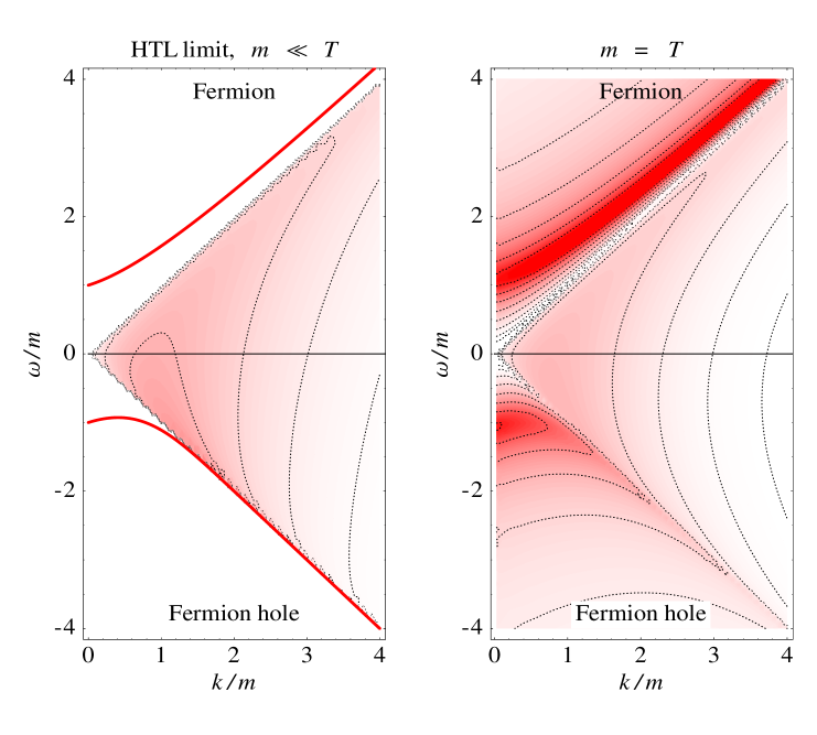
Figure 7: Spectral density of a massless fermion in a thermal plasma, plotted in HTL approximation ($g\ll 1$, i.e. thermal mass $m\sim gT\ll T$) and beyond. Notice the main differences: the particle ($\omega>0$) and ‘holes’ ($\omega<0$) poles develop a finite width, and, more importantly, the continuum below the light-cone gets Boltzmann suppressed at $k\,\raise 1.29167pt\hbox{$>$\kern-7.5pt\lower 4.30554pt\hbox{$\sim$}}\,T$. Contours are equispaced in $\log$ scale.

3.2 Full one loop thermal effects

The HTL approximation holds at momenta and energies $k,\omega\ll T$, correctly describing thermal effects that arise at $k,\omega\sim gT$ if $g\ll 1$. However, the physically relevant values of gauge couplings (especially the strong coupling) are not small enough to justify the use of the HTL approximation. We therefore use the full one-loop thermal and quantum corrections to propagators of scalars, fermions and vectors. Explicit expressions are collected in appendices B and LABEL:thermalF (see also [WeldonFermion, WeldonVector, thoma, LeBellac]) and fig. 7 illustrates (in the case of a massless fermion) the qualitatively new effects that arise beyond the HTL limit.

The most visible effect (although not the most important one) happens at $|\omega|>k$ i.e. ‘above the light cone’. In the $g\to 0$ limit particles (and quasi-particles such as fermion ‘holes’) have an infinitesimal width: their dispersion relations are plotted as thin lines in fig. 7a. For finite $g$ they get a finite width $\Gamma$ (both from $T=0$ quantum effects and from thermal effects), such that their spectral density gets smeared acquiring the usual bell-like shape. This is why a continuum appears also above the light cone in fig. 7b. A well known problem encountered in thermal computations is that sometimes thermal effects give $\Gamma<0$. We therefore included the $T=0$ contribution, finding that the total $\Gamma$ is positive for scalars and fermions. This cure does not work for vectors, because the $T=0$ contribution to their $\Gamma$ can itself be negative depending on the gauge choice, see eq. (LABEL:eq:pi0). We therefore think that the negativity of $\Gamma$ is not related to higher-order subtleties in the thermal expansion, but just to gauge invariance. It should not affect computations of physical gauge-invariant quantities, provided that one can do an exact computation up to some order in the perturbative expansion. The only trouble is that in practice it is difficult to achieve this in finite temperature computations. In view of this situation, since the would-be poles are anyhow reasonably narrow for the physical values of the coupling that enter our computation, we use for them the HTL approximation. Notice that the HTL approximation correctly describes the position of the poles (i.e. the dispersion relations) even at large $k\,\raise 1.29167pt\hbox{$>$\kern-7.5pt\lower 4.30554pt\hbox{$\sim$}}\,T$: poles lie close to the light-cone, $|\omega|\approx k$, even if $g\sim 1$ [thoma].

The new effect important for our purposes arises at $|\omega|<k$, i.e. ‘below the light cone’. Quantum effects do not give any contribution to spectral densities here (and more generally below the threshold for zero-temperature decays), and the purely thermal contribution is not problematic. Even in HTL approximation, thermal effects give non zero spectral densities below the light cone: this describes ‘Landau damping’ i.e. the fact that particles exchange energy with the thermal plasma. However the HTL approximation cannot be applied at $k\sim T$ (a region relevant for us, since $g\sim 1$), and indeed it misses one key physical fact: at $k\gg T$ spectral densities get suppressed by an exponential Boltzmann factor. Indeed the thermally averaged coupling of a particle with large momentum $k\gg T$ is small, since very few of the particles in the plasma have the large momentum demanded by energy-momentum conservation. This Boltzmann suppression of the spectral density below the light cone is the main difference between fig. 7a (HTL approximation) and fig. 7b (full one loop), and makes the gravitino production rate about $50\%$ smaller than what one would find by applying the HTL approximation at all momenta, outside its domain of validity $p\ll T$.

3.3 Vector and gaugino propagators

We are now going to present how spectral densities are practically used. We need the resummed propagators for the vector with four-momentum $K=(k_{0},\mbox{\normalsize\boldmath$k$})$ and the gaugino with four-momentum $Q=(q_{0},\mbox{\normalsize\boldmath$q$})$ in the loop. We employ non-time ordered propagators (as they allow slightly cleaner formulæ than imaginary parts of propagators), denoted with a ${}^{<}$ in the notation of [LeBellac] that we follow. Thermally resummed propagators are denoted with a ${}^{*}$: they are (see appendices B, LABEL:thermalF for more details)

$$\halign to=0.0pt{\@eqnsel\hskip\@centering$\displaystyle{#}$&\global\@eqcnt\@ne\hskip 2\arraycolsep\hfil${#}$\hfil& \global\@eqcnt\tw@\hskip 2\arraycolsep$\displaystyle{#}$\hfil&\llap{#}\cr 0.0pt plus 1000.0pt$\displaystyle{{}^{*}S^{<}(Q) &10.0pt\hfil${=&10.0pt$\displaystyle{\frac{f_{F}(q_{0})}{2}\bigg{[}(\gamma_{0} - \mbox{\normalsize\boldmath$\gamma$}\cdot\hat{\mbox{\normalsize\boldmath$q$}}) \rho_{+}(Q)+(\gamma_{0} + \mbox{\normalsize\boldmath$\gamma$}\cdot\hat{\mbox{\normalsize\boldmath$q$}}) \rho_{-}(Q)\bigg{]}, \\ ^{*}D_{\mu\nu}^{<}(K) &\hbox to0.0pt{\hss=&f_{B}(k_{0})\bigg{[}\Pi_{\mu\nu}^{T}\rho_{T}(K)+\Pi_{\mu\nu}^{L}\frac{|\mbox{\normalsize\boldmath$k$}|^{2}}{K^{2}}\rho_{L}(K)+\xi\frac{k_{\mu}k_{\nu}}{K^{4}}\bigg{]}.&(3.5)\cr}}}}}$$

Some explanations are in order. First, $q_{0}>0$ or $k_{0}>0$ describes a fermion or a vector in the final state, and $q_{0}<0$ or $k_{0}<0$ describes a fermion or a vector in the initial state: this convention allows to compactly describe all possible processes. Indeed the factors

$$\halign to=0.0pt{\@eqnsel\hskip\@centering$\displaystyle{#}$&\global\@eqcnt\@ne\hskip 2\arraycolsep\hfil${#}$\hfil& \global\@eqcnt\tw@\hskip 2\arraycolsep$\displaystyle{#}$\hfil&\llap{#}\cr 0.0pt plus 1000.0pt$\displaystyle{f_{B}(k_{0})&10.0pt\hfil${\equiv&10.0pt$\displaystyle{\frac{1}{e^{k_{0}/T}-1} = \left\{\begin{array}[]{ll}n_{B}&\hbox{if $k_{0}>0$}\\ -(1+n_{B})&\hbox{if $k_{0}<0$}\end{array}\right.\\ f_{F}(q_{0})&\hbox to0.0pt{\hss\equiv&\frac{1}{e^{q_{0}/T}-1}=\left\{\begin{array}[]{ll}n_{F}&\hbox{if $q_{0}>0$}\\ 1-n_{F}&\hbox{if $q_{0}<0$}\end{array}\right.&(3.6)\cr}}}}}$$

give the usual statistical factors: $-n$ (number of particles in the initial state) or $1\pm n$ (stimulated emission or Pauli-blocking in the final state), where $n_{B,F}(E)\equiv 1/(e^{|E|/T}\mp 1)$ are the usual Bose-Einstein and Fermi-Dirac distributions.

Second, $\rho_{+}$, $\rho_{-}$, $\rho_{T}$, $\rho_{L}$ are the spectral densities for the fermion, fermion pole, transverse vectors and longitudinal vectors respectively. As discussed in the previous section, we can keep the HTL pole approximation outside the light cone, so that

$$\halign to=0.0pt{\@eqnsel\hskip\@centering$\displaystyle{#}$&\global\@eqcnt\@ne\hskip 2\arraycolsep\hfil${#}$\hfil& \global\@eqcnt\tw@\hskip 2\arraycolsep$\displaystyle{#}$\hfil&\llap{#}\cr 0.0pt plus 1000.0pt$\displaystyle{\rho_{\pm}(Q) &10.0pt\hfil${=&10.0pt$\displaystyle{2\pi\bigg{[}Z_{\pm}(q)\,\delta(q_{0}-\omega_{\pm}(q))+Z_{\mp}\, \delta(q_{0}+\omega_{\mp}(q))\bigg{]} + \rho_{\pm}^{\rm cont}(Q),\\ \rho_{L,T}(K) &\hbox to0.0pt{\hss=&2\pi\bigg{[}Z_{L,T}(k)\,\delta(k_{0}-\omega_{L,T}(k))-Z_{L,T}\,\delta(k_{0}+\omega_{L,T}(k))\bigg{]}+\rho_{L,T}^{\rm cont}(Q).&(3.7)\cr}}}}}$$

In HTL approximation the residues at the poles are given in terms of the pole positions $\omega_{\pm}(q)$ and $\omega_{L,T}(k)$ as [WeldonVector, WeldonFermion, LeBellac]

$$Z_{\pm}=\frac{\omega_{\pm}^{2}-q^{2}}{2m_{F}^{2}},\qquad Z_{L}=\frac{\omega_{L}(\omega_{L}-k^{2})}{k^{2}(k^{2}+2m_{V}^{2}-\omega_{L}^{2})},\qquad Z_{T}=\frac{\omega_{T}(\omega_{T}^{2}-k^{2})}{2m_{V}^{2}\omega_{T}^{2}-(\omega_{T}^{2}-k^{2})^{2}}.$$ (3.8)

These formulæ tell that residues for longitudinal and hole excitations are exponentially suppressed at energies larger than $gT$: they are low-energy collective phenomena. The continua $\rho^{\rm cont}$ only exist below the light cone, at $|q_{0}|<q$ and $|k_{0}|<k$. The spectral densities satisfy sum rules such as

$$\int_{-\infty}^{+\infty}\frac{dq_{0}}{2\pi}\rho_{\pm}(Q)=1,\qquad\int_{-\infty}^{+\infty}\frac{dk_{0}}{2\pi}\rho_{T}(K)=1,\qquad\int_{-\infty}^{+\infty}\frac{dk_{0}}{2\pi}\rho_{L}(K)=\frac{2m_{V}^{2}}{3k^{2}}$$ (3.9)

and the continuum turns out to contribute $\sim(10\div 20)\%$ less than the poles. Eq. (3.9) means that the number density of longitudinal vectors diverges at $k\to 0$, but this leaves finite gravitino rates thanks to the $d^{3}k$ integration factor. In the $T=0$ limit $\omega_{\pm}(q)=\pm q$, $\omega_{L,T}(k)=k$ and one can check that the standard expressions for the propagators are recovered. Notice that $\rho_{L,T}$ have dimensions mass${}^{-2}$, while $\rho_{\pm}$ have dimensions mass${}^{-1}$.

4 Gravitino production rate due to decay effects

We can now compute the imaginary part of diagram D in fig. 3, and extract from it the gravitino production rate. Using the gravitino $\leftrightarrow$ Goldstino equivalence, eq. (2.4), diagram D is obtained from eq. (2.2) by inserting the quadratic parts of the MSSM supercurrent (A.28) and of its divergence (A.29):

$$S_{(2)}^{\mu} =-\sum_{N=1}^{3}\frac{1}{4}F_{\nu\rho}^{(N)}[\gamma^{\nu},\gamma^{\rho}]\gamma^{\mu}\gamma^{5}\lambda^{(N)}-\sqrt{2}\left[(\partial^{\nu}\phi_{i})^{\ast}(\gamma^{\nu}\gamma^{\mu}\xi_{L}^{i})+(\partial^{\nu}\phi_{i})(\gamma^{\nu}\gamma^{\mu}\xi_{R}^{i})\right],$$

$$(\partial\cdot S)_{(2)} =-\sum_{N=1}^{3}\frac{M_{N}}{4}{\cal O}_{N},\qquad{\cal O}_{N}=F_{\mu\nu}^{(N)}[\gamma_{\mu},\gamma_{\nu}]i\gamma^{5}\lambda^{(N)}$$

where $N$ runs over the three factors of the MSSM gauge group, and $F_{\nu\rho}^{(N)}$ here stands for the linearized part of the corresponding field strength. We ignored soft-breaking squared masses of scalars, as they have higher dimension than gaugino masses $M_{N}$. The contribution to $\Pi^{<}$ from diagram D is

$$\Pi^{<}(P) =\frac{1}{4\bar{M}_{\mathrm{Pl}}^{2}}\left[\mathrm{Tr}\langle{\bar{S}}_{(2)}^{\mu}\Pi^{3/2}_{\mu\nu}S_{(2)}^{\nu}\rangle_{T}-\frac{2}{3m_{3/2}^{2}}\mathrm{Tr}\langle(\partial\cdot\bar{S})_{(2)}P/\,(\partial\cdot S)_{(2)}\rangle_{T}\right]$$ (4.1)

$$=\sum_{N=1}^{3}\frac{1}{32\bar{M}_{\mathrm{Pl}}^{2}}\left(1+\frac{M_{N}^{2}}{3m_{3/2}^{2}}\right)\mathrm{Tr}\langle\bar{{\cal O}}_{N}P/\,{\cal O}_{N}\rangle_{T}.$$ (4.2)

We now explain how eq. (4.2) is obtained. The Goldstino part, proportional to $M_{N}^{2}/3m_{3/2}^{2}$, is straightforward. We emphasize that the divergence of the supercurrent is evaluated before evaluating its thermal matrix element. Indeed, while thermal masses naïvely look like SUSY-breaking terms of order $g^{2}T$, they actually do not contribute to $\partial_{\mu}S^{\mu}$, and a mistake about this issue would make the Goldstino rate qualitatively wrong [wrong, LR, Ellis] (see also appendix A). Indeed, despite the nice formalism employed to compute them (periodic and anti-periodic boundary conditions in imaginary time for bosons and fermions respectively), thermal effects just are one particular background: no background affects the operator equations of motion, such that a supercurrent which is conserved at $T=0$ remains conserved at finite $T$.

For the remaining massless gravitino part, we insert the explicit value of the gravitino polarization tensor (2.5) and get two terms of the form

$$\mathrm{Tr}\langle{\bar{S}}_{(2)}^{\mu}P/\,S_{(2)}^{\mu}\,\rangle_{T}+\frac{1}{2}\mathrm{Tr}\langle S/\,_{(2)}P/\,\overline{S/\,}_{(2)}\,\rangle_{T}$$ (4.3)

where ${}S/\,_{(2)}\equiv\gamma_{\mu}{}\,S_{(2)}^{\mu}$. We can now perform simplifications that only employ the known Dirac-matrix structure of ${S}_{(2)}^{\mu}$:

• The vector/gaugino contributions obey $S/\,_{(2)}=0$ (thanks to $\gamma_{\mu}[\gamma_{\alpha},\gamma_{\beta}]\gamma^{\mu}=0$), such that only the first term of eq. (4.3) contributes. It is reduced to the same operator ${\cal O}_{N}$ using the $\gamma_{\mu}\gamma_{\alpha}\gamma^{\mu}=-2\gamma_{\alpha}$ identity and taking into account that the thermally corrected gluino propagator has the same $\gamma$-matrix structure as the massless propagator. This leads to the $1+M_{N}^{2}/3m_{3/2}^{2}$ prefactor in eq. (4.2).

• The quark/squark contributions vanish, thanks to a cancellation between the two terms in eq. (4.3). Indeed, by applying the $\gamma_{\mu}\gamma_{\alpha}\gamma^{\mu}=-2\gamma_{\alpha}$ identity (one time in the first term, and two times in the second term) both terms reduce to the matrix element $\mathrm{Tr}\langle\bar{\xi}_{R}(\partial\!\!\!\raisebox{2.0pt}[0.0pt][0.0pt]{$\scriptstyle/$}\,\varphi)P/\,(\partial\!\!\!\raisebox{2.0pt}[0.0pt][0.0pt]{$\scriptstyle/$}\,\varphi^{\ast})\xi_{L}\rangle$, with opposite coefficients.

We don’t know if there is some deeper reason dictating these cancellations such that the full result is controlled by the thermal matrix element of the operator ${\cal O}_{N}$ times the prefactor $1+M_{N}^{2}/3m_{3/2}^{2}$. A general proof of this result would allow to get the full production rate from the simple Goltstino rate according to eq. (4.2).

For completeness we mention that we have studied thermal corrections to the ${\cal O}_{N}$ operators in HTL approximation. As well known gauge vertices $g$ receive very large thermal corrections of order $g(1+g^{2}T^{2}/k^{2})$ where $k\ll T$ (HTL approximation) is some external momentum: their presence would be problematic, as they seem to describe infra-red divergent effects (see e.g. section 10.3 of [LeBellac]). In the case of gauge vertices these corrections are demanded by gauge invariance: different diagrams combine such that $\mathscr{L}_{\rm HTL}$ of eq. (3.1) contains the gauge-covariant derivative $D$. On the contrary Yukawa couplings do not receive these problematic HTL corrections. We verified that the Goldstino vertex $\chi{\cal O}_{N}$ does not receive any HTL correction. Beyond the HTL limit there will be corrections suppressed by powers of $g/\pi$, that we can ignore.

4.1 Gravitino propagator

We now restart from eq. (4.2) and explicitly compute the imaginary part of the gravitino propagator with four-momentum $P=(p_{0},\mbox{\normalsize\boldmath$p$})=K+Q$, summed over its polarizations:

$$\Pi^{<}(E)=\sum_{N=1}^{3}\bigg{(}1+\frac{M_{N}^{2}}{3m_{3/2}^{2}}\bigg{)}\frac{n_{N}}{16(2\pi)^{2}\bar{M}_{\rm Pl}^{2}}\int\frac{d^{4}K}{(2\pi)^{4}}{\rm Tr}[P/\,[K/,\gamma_{\mu}]i\gamma_{5}{}^{*}{\!}S^{<}(Q)i\gamma_{5}[-K/,\gamma_{\nu}]^{*}D_{\mu\nu}(K)].$$ (4.4)

where $N=\{1,2,3\}$ runs over the three factors of the SM gauge group with $n_{N}=\{1,3,8\}$ vectors; $M_{N}$ are the gaugino masses at zero temperature (renormalized at some scale around $T$). Inserting the explicit parameterization

$$K=(k_{0},k,0,0),\qquad Q=(q_{0},q\cos\theta_{q},q\sin\theta_{q}),\qquad P=(p,p\cos\theta_{p},p\sin\theta_{p})$$

for the vector, gaugino and gravitino four-momenta respectively one finds

$$\Pi^{<}(p) = \sum_{N=1}^{3}p\bigg{(}1+\frac{M_{N}^{2}}{3m_{3/2}^{2}}\bigg{)}\frac{n_{N}}{\bar{M}_{\rm Pl}^{2}}\int\frac{d^{4}K}{(2\pi)^{4}}f_{B}(k_{0})f_{F}(q_{0})\times$$

$$\bigg{[}\rho_{L}(K)\rho_{-}(Q)k^{2}\cos^{2}\frac{\theta_{p}+\theta_{q}}{2}+\rho_{L}(K)\rho_{+}(Q)k^{2}\sin^{2}\frac{\theta_{p}+\theta_{q}}{2}+$$

$$+\rho_{T}(K)\rho_{+}(Q)\bigg{(}(k^{2}+k_{0}^{2})(1+\cos\theta_{p}\cos\theta_{q})-2kk_{0}(\cos\theta_{p}+\cos\theta_{q})\bigg{)}+$$

$$+\rho_{T}(K)\rho_{-}(Q)\bigg{(}(k^{2}+k_{0}^{2})(1-\cos\theta_{p}\cos\theta_{q})-2kk_{0}(\cos\theta_{p}-\cos\theta_{q})\bigg{)}\bigg{]}$$

To compute the total rate $\gamma_{D}$ using eq. (2.1) it is convenient to multiply by $1=\int d^{4}Q~{}\delta^{4}(K-P-Q)$, perform the non-trivial angular integrations over $\theta_{p}$ and $\theta_{q}$, obtaining

$$\gamma_{D}=\frac{T^{6}}{2(2\pi)^{3}\bar{M}_{\rm Pl}^{2}}\sum_{N=1}^{3}n_{N}\bigg{(}1+\frac{M_{N}^{2}}{3m_{3/2}^{2}}\bigg{)}f_{N},$$ (4.6)

where

$$f_{N} = T^{-6}\int_{-\infty}^{+\infty}dq_{0}~{}dk_{0}~{}kf_{B}(k_{0})f_{F}(q_{0})\times$$

$$\times\bigg{[}\rho_{L}(K)\rho_{-}(Q)(p-q)^{2}[(p+q)^{2}-k^{2}]+\rho_{L}(K)\rho_{+}(Q)(p+q)^{2}[k^{2}-(p-q)^{2}]+$$

$$+\rho_{T}(K)\rho_{+}(Q)((p+q)^{2}-k^{2})\bigg{(}(1+k_{0}^{2}/k^{2})(k^{2}+(p-q)^{2})-4k_{0}(p-q)\bigg{)}+$$

$$+\rho_{T}(K)\rho_{-}(Q)(k^{2}-(p-q)^{2})\bigg{(}(1+k_{0}^{2}/k^{2})(k^{2}+(p+q)^{2})-4k_{0}(p+q)\bigg{)}\bigg{]}.$$

The dimensionless coefficients $f_{N}$ are positive: each term in the square brackets is positive in the allowed region, except $\rho_{T}$ that becomes positive after being multiplied by $f_{B}(k_{0})$. The integration range is restricted by momentum conservation, $\mbox{\normalsize\boldmath$p$}+\mbox{\normalsize\boldmath$k$}+\mbox{\normalsize\boldmath$q$}=0$, i.e.  $|k-q|\leq p=k_{0}+q_{0}\leq k+q$: any side of a triangle cannot be longer than the sum of the other two or shorter than their difference.

The last two equations generalize eq. (38) of [Buch], who considered the vector/gaugino loop in the limit of hard gravitino and soft vector (small $k_{0}\ll p,T$, such that $f_{B}(k_{0})\simeq T/k_{0}$) and neglected the gaugino thermal mass (i.e. $\rho_{-}\simeq 0$ and $\rho_{+}\simeq 2\pi\delta(q_{0}-q)$ such that $q=q_{0}=p-k_{0}$).

4.2 Decay contribution to the gravitino production rate

In conclusion, the decay contribution to the gravitino production rate per space-time volume is given by eq. (4.6). The coefficients $f_{N}$ have to be evaluated numerically. We approximate the spectral densities outside the light cone as $\delta$-function poles (using full expressions they would be narrow bells, making numerical integration difficult for our limited computing power), such that we have four types of contributions: pole-pole, continuum-continuum, (vector pole)-(gaugino continuum) and (vector continuum)-(gaugino pole). A vector can be either longitudinal or transverse, in the initial state or in the final state, and similarly for the gaugino.

The resulting coefficients $f_{N}$ depend on the gauge couplings and on the content of matter charged under the given gauge group; in the MSSM it is convenient to parametrize them as functions of the thermal vector masses $m_{V_{N}}$ listed in eq. (3.3):

$$f_{N}\equiv f_{N}(\frac{m_{V_{N}}}{T}).$$ (4.8)

For example $m_{3}\approx 1.3T$ for the gluon at $T\approx 10^{9}\,{\rm GeV}$. The functions $f_{N}$ are plotted in fig. 1. In HTL approximation there would be a unique $N$-independent function $f$, and the functions $f_{N}$ turn out to be somewhat different, depending on the relative amount of vector and chiral multiplets present within each group. In non-minimal models with more chiral multiplets than in the MSSM, one would have to add their extra contributions to vector thermal masses, and to slightly revise the functions $f_{N}$.

Finally, let us try to discuss the accuracy of our result. Thermal corrections to the pressure have been computed up to high orders in $g_{3}$ [largeNf]: these computations can be used to see how convergent the perturbative expansion is in practice. In the favorable limit $N_{f}\gg N_{c}$ (where $N_{f}$ is the number of flavors and $N_{c}$ is the number of colors) the perturbative expansion for the pressure remains accurate up to $m_{V}/T\approx 1$ (fig. 1 of [largeNf]). This presumably also applies to our case, as SUSY-QCD has a set of fermions and scalars that give the same contribution to the gluon thermal mass as $N_{f}=21$ flavors in the fundamental.

Furthermore, AdS/CFT techniques should allow to compute the large coupling limit of the gravitino emission rate in some supersymmetric theory, maybe not unrealistically different from SUSY-QCD. This could be done analogously to how [Starinets] used AdS/CFT to compute the photon emission rate from strongly coupled $\mathcal{N}=4$ SYM in the large $N_{c}$ limit. By analogy, we expect that at strong coupling the gravitino rate functions $f_{N}$ will have a finite limit, $N_{c}$-independent up to $1/N_{c}$ corrections.

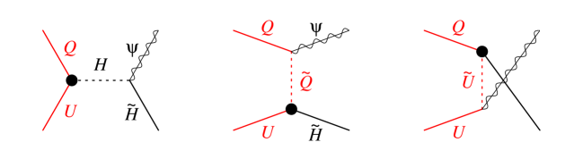
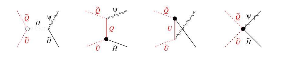
Figure 8: Top scatterings. Feynman diagrams contributing to $QU\to\Psi_{\mu}\tilde{H}$. The $\bullet$ denotes the top Yukawa coupling.

Figure 9: Top scatterings. Feynman diagrams contributing to $\tilde{Q}\tilde{U}\to\Psi_{\mu}\tilde{H}$. The $\bullet$ denotes a coupling proportional to $\lambda_{t}$, and $\circ$ its $A$-term.

5 Production of gravitinos due to the top Yukawa

Previous works considered gravitino production due to the $g_{3}$, $g_{2}$ and $g_{Y}$ gauge couplings; the top quark Yukawa, $\lambda_{t}~{}QUH$, also has a sizable coupling $\lambda_{t}$. There are two main kind of scattering processes:

• Scatterings involving fermions only, such as $QU\to\Psi\tilde{H}$: fig. 9 shows the relevant Feynman diagrams. They would populate only the spin 3/2 component of the gravitino, as only dimension-2 soft terms enter these diagrams, so that Goldstinos are not produced. However, an explicit computation shows that the dominant contribution, of order $T^{6}/M_{\rm Pl}^{2}$, vanishes.

• Scatterings involving two fermions and two scalars, such as $\tilde{Q}\tilde{U}\to\Psi\tilde{H}$: fig. 9 shows the relevant Feynman diagrams. The first diagram involves $A_{t}$, the dimension-1 $A$-term of the top Yukawa coupling, and populates the spin 1/2 component of the gravitino. The other three diagrams populate the spin 3/2 component.

The total result is:

$$\sum_{\rm all}|\mathscr{A}(\hbox{top scatterings})|^{2}=72\frac{\lambda_{t}^{2}}{\bar{M}_{\rm Pl}^{2}}(1+\frac{A_{t}^{2}}{3m_{3/2}^{2}})s$$ (5.1)

where $s=(P_{1}+P_{2})^{2}$ is the usual kinematical variable. The corresponding gravitino production rate is

$$\gamma_{\rm top}=1.30\frac{9\lambda_{t}^{2}T^{6}}{2\bar{M}_{\rm Pl}^{2}\pi^{5}}(1+\frac{A_{t}^{2}}{3m_{3/2}^{2}})$$ (5.2)

where the numerical factor $1.30$ is the correction due to the Fermi-Dirac and Bose-Einstein factors with respect to the Boltzmann approximation.

In the language of previous sections, eq. (5.2) is the scattering contribution. We now explain why it also is our total result. First, it happens to be infra-red convergent: the potentially divergent contributions given by the modulus squared of the $t$-channel and $u$-channel diagrams in fig. 9 actually vanish. Therefore, unlike in the case of gauge scatterings, the inclusion of thermal masses is not necessary for obtaining a finite result. Furthermore, including thermal effects along the lines of the previous sections does not affect the final result. Indeed the top Yukawa coupling gives a thermal mass for top, stops (and higgs and higgsinos): the resulting quark/squark/gravitino (and higgs/higgsino/gravitino) decay rates have been computed in section 4 for generic thermal masses, and vanish. Consistency requires that the subtracted top scattering rate equals the total scattering rate of eq. (5.2), and indeed the subtracted terms are the modulus squared of the $t$-channel and $u$-channel diagrams in fig. 9, which vanish.

Again, all these cancellations have a simple interpretation: they are the ones needed such that the production rate for the spin 3/2 components of the gravitino equals the production rate for the spin 1/2 Goldstino components, up to the prefactor in eq. (5.1). Indeed, using the gravitino/Goldstino equivalence, the Goldstino production rate can be equivalently computed from one single diagram that only involves the single quartic Goldstino coupling,

$$A_{t}\lambda_{t}~{}\hbox{Goldstino}~{}(\hbox{higgsino}~{}\hbox{squark}~{}\hbox{squark}^{*}+\hbox{quark}~{}\hbox{squark}^{*}~{}\hbox{higgs}+\hbox{h.c.}),$$

such that decay contributions and subtracted scattering rates simply do not exist for the Goldstino.

Figure 10: Evolution of the gravitino abundancy $n/s$ in units of $\gamma/H_{R}s$ at $T=T_{\rm RH}$ for naïve instant reheating and for the conventional model of reheating.

6 Boltzmann equations with reheating

We here compute the gravitino abundance by integrating the relevant Boltzmann equations. While previous works ignored the history of the universe prior to its reheating (from the point of view of computing gravitino production this in practice amounts to assuming that the Big Bang started at the maximal temperature $T_{\rm RH}$), we here follow the standard definition of the reheating temperature $T_{\rm RH}$, where MSSM particles are progressively reheated by the energy released by some non-relativistic energy density $\rho_{\phi}$, which could describe e.g. an oscillating inflaton field, or some non-relativistic particle decaying into MSSM particles. In both cases the relevant Boltzmann equations are

$$\left\{\begin{array}[]{l}\dot{\rho}_{\phi}+3H\rho_{\phi}=-\Gamma_{\phi}\rho_{\phi}\cr\dot{\rho}_{R}+4H\rho_{R}=\Gamma_{\phi}\rho_{\phi}\cr\dot{n}_{3/2}+3Hn_{3/2}=\gamma\end{array}\right.$$ (6.1)

where $n_{3/2}$ is the gravitino number density summed over its polarizations, a dot denotes $d/dt$, $H=\dot{R}/R=\sqrt{8\pi(\rho_{\phi}+\rho_{R})/3}/M_{\rm Pl}$ is the expansion factor, $\rho_{R}=\pi^{2}g_{*}T^{4}/30$ is the energy density of MSSM radiation at temperature $T$ (with $g_{*}=228.75$, up to ${\cal O}(g^{2})$ corrections, and up to adding right-handed neutrinos), and $\Gamma_{\phi}$ parameterizes the decay width of $\rho_{\phi}$. The reheating temperature $T_{\rm RH}$ is defined in terms of $\Gamma_{\phi}$ as the temperature at which [book]

$$\Gamma_{\phi}=H_{R}\equiv\frac{1}{M_{\rm Pl}}\sqrt{\frac{8\pi}{3}\rho_{R}(T_{\rm RH})}\qquad\hbox{i.e.}\qquad T_{\rm RH}=\left[\frac{45}{4\pi^{3}g_{*}}\,\Gamma_{\phi}^{2}M_{\rm Pl}^{2}\right]^{1/4}.$$ (6.2)

It is convenient to rewrite equations (6.1) in terms of $Y(z)$, where $z\equiv T_{\rm RH}/T$ and $Y\equiv n_{3/2}/s$, with $s=4\rho_{R}/3T$ being the MSSM entropy density. Following [leptog] one gets

$$\left\{\begin{array}[]{rcl}\displaystyle HZz\frac{d\rho_{\phi}}{dz}&=&-{3H\rho_{\phi}}-{\Gamma_{\phi}\rho_{\phi}}\,,\\[11.38109pt] \displaystyle sHZz\frac{dY}{dz}&=&3sH(Z-1)Y+\gamma\end{array}\right.$$ (6.3)

where

$$Z=-\frac{\dot{\rho}_{R}}{4\rho_{R}H}=1-\frac{\Gamma_{\phi}\rho_{\phi}}{4H\rho_{R}}.$$ (6.4)

To clarify the physical meaning of $T_{\rm RH}$, we emphasize that $T_{\rm RH}$ is not the maximal temperature; however what happens at $T\gg T_{\rm RH}$ gets diluted by the entropy release described by the $Z-1$ factor ($Z\simeq 3/8$ at $T\gg T_{\rm RH}$ and $Z\simeq 1$ at $T\ll T_{\rm RH}$). In our case $\gamma(T)\propto T^{6}$ and the solution is

$$Y(T\ll T_{\rm RH})=2\left.\frac{\gamma}{Hs}\right|_{T=T_{\rm RH}}=0.745\left.\frac{\gamma}{H_{R}s}\right|_{T=T_{\rm RH}}=6.11~{}10^{-12}\frac{T_{\rm RH}}{10^{10}\,{\rm GeV}}\frac{\gamma|_{T=T_{\rm RH}}}{T_{\rm RH}^{6}/\bar{M}_{\rm Pl}^{2}}.$$ (6.5)

Fig. 12 shows our results for the dimensionless order-one combination $\gamma/(T^{6}/\bar{M}_{\rm Pl}^{2})$ that appears in  (6.5). Notice that the gravitino abundance is proportional to it, and to $T_{\rm RH}$: the large power $\gamma(T)\propto T^{6}$ gets almost compensated by cosmological factors.

In previous analyses $\rho_{\phi}$ was ignored and the ‘instantaneous reheating’ approximation was used, which amounts to start the Big Bang from a maximal temperature $T=T_{\rm RH}$: this gives a slightly larger gravitino abundance

$$Y(T\ll T_{\rm RH})=\left.\frac{\gamma}{H_{R}s}\right|_{T=T_{\rm RH}}.$$ (6.6)

Fig. 10 illustrates the different evolution of $Y$ (in arbitrary units) between the two cases.

Within the standard $\Lambda$CDM cosmological model, present data demand a DM energy density $\Omega_{\rm DM}h^{2}=0.110\pm 0.006$; if DM are non relativistic particles with mass $M\gg{\rm keV}$ this corresponds to $Y_{\rm DM}=(0.40\pm 0.02)\,{\rm eV}/M$ [WMAP]. One has $Y=Y_{\rm DM}$ if gravitinos are the observed DM. Equivalently, one can compute the present gravitino mass density in terms of their relative entropy $Y$ as

$$\Omega_{3/2}h^{2}=\frac{m_{3/2}Ys_{0}}{\rho_{\rm cr}/h^{2}}=0.274~{}10^{9}~{}Y\frac{m_{3/2}}{\,{\rm GeV}}=0.00167\frac{m_{3/2}}{\,{\rm GeV}}\frac{T_{\rm RH}}{10^{10}\,{\rm GeV}}\frac{\gamma|_{T=T_{\rm RH}}}{T_{\rm RH}^{6}/\bar{M}_{\rm Pl}^{2}}.$$ (6.7)

where $\rho_{\rm cr}=3H_{0}^{2}M_{\rm Pl}^{2}/8\pi$ is the critical energy density, $H_{0}=100\,h\,\hbox{km/sec$\cdot$Mpc}$ is the Hubble constant, the present entropy density is $s_{\rm 0}=2\pi^{2}g_{*s}T_{0}^{3}/45$ with $g_{*s}=43/11$ and $T_{0}=2.725\,{\rm K}$. Fig. 11 compares the regions where the thermal gravitino abundance equals the DM abundance with the regions compatible with standard thermal leptogenesis [DI], as computed in [leptog] with the same definition of the reheating process. This plot ignores all model dependent issues, including who is the LSP and the NLSP. Let us briefly summarize these issues [gravitinoCosmo, Moroi, Viel, altri].

• If the gravitino is the stable LSP then

  • if $m_{3/2}\gg{\rm keV}$ the gravitino behaves as cold dark matter and its energy density can be at most equal to the DM density.

  • a somewhat stronger constraint applies if the gravitino is lighter, $T_{0}\ll m_{3/2}\,\raise 1.29167pt\hbox{$<$\kern-7.5pt\lower 4.30554pt\hbox{$\sim$}}\,{\rm keV}$, and consequently behaves as warm dark matter or radiation. The Goldstino component of such a light gravitino thermalizes (unless $T_{\rm RH}$ is as low as possible), so that this scenario is severely constrained: assuming that the Goldstino was in thermal equilibrium when $g_{*}\sim 100$, present data demand $m_{3/2}\,\raise 1.29167pt\hbox{$<$\kern-7.5pt\lower 4.30554pt\hbox{$\sim$}}\,16\,{\rm eV}$ [Viel].

  An additional contribution to the gravitino energy density, $\Omega_{3/2}^{\rm extra}\simeq\Omega_{\rm NLSP}m_{3/2}/m_{\rm NLSP}$ (having neglected entropy production, which typically is an excellent approximation) is generated by NLSP decays, with mass $m_{\rm NLSP}$ and mass density $\Omega_{\rm NLSP}$ after their freeze-out. Weak scale sparticles give $\Omega_{\rm NLSP}\sim 1$, such that this extra contribution is significant if $m_{3/2}$ is not much smaller than $m_{\rm NLSP}$.

• If heavier than the LSP (which possibly has mass $m_{\rm LSP}\sim 100\,{\rm GeV}$), the gravitino gravitationally decays into the LSP and some SM particles:

  • If $m_{3/2}\gg 10\,{\rm TeV}$ the gravitino decays before BBN, generating a contribution to the LSP energy density, $\Omega_{\rm LSP}\simeq m_{\rm LSP}\Omega_{3/2}/m_{3/2}$ [gravitinoCosmo] (we neglected the entropy in gravitinos).

  • A lighter gravitino decays during or after BBN, damaging nucleosynthesis. The resulting bound on $\Omega_{3/2}$ depends on which SM particles are produced by gravitino decays, and typically is some orders of magnitude stronger than the DM bound $\Omega_{3/2}h^{2}\,\raise 1.29167pt\hbox{$<$\kern-7.5pt\lower 4.30554pt\hbox{$\sim$}}\,0.1$ [Moroi]. Very late gravitino decay into photons would also distort the CMB energy spectrum.

We recall that we computed thermal production of gravitinos from MSSM particles at temperatures $T_{\rm RH}\gg m_{3/2},m_{\rm soft}$. The true physics might be different. For example, the messenger fields with mass $M_{\rm GM}$ employed by gauge mediation models might be so light that they get thermalized (together with the hidden sector) and later decay back to MSSM particles, leaving a thermalized Goldstino. Eq. (6.3) shows that this phenomenon is dominant if $M_{\rm GM}\,\raise 1.29167pt\hbox{$<$\kern-7.5pt\lower 4.30554pt\hbox{$\sim$}}\,(10\div 100)T_{\rm RH}$, as the gravitino abundance gets washed-out as $Y\propto T^{5}$ during reheating at $T\,\raise 1.29167pt\hbox{$>$\kern-7.5pt\lower 4.30554pt\hbox{$\sim$}}\,T_{\rm RH}$.

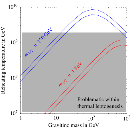
Figure 11: The bands show the region where the thermal gravitino abundance equals the DM abundance ($3\sigma$ regions), assuming unified gaugino masses with $m_{1/2}=150\,{\rm GeV}$ (roughly the minimal value allowed by present data) or $m_{1/2}=1\,{\rm TeV}$ at the unification scale, and negligible $A_{t}$. Model-dependent issues are here ignored, including who is the LSP and the NLSP. Successful thermal leptogenesis with zero initial right-handed neutrino abundance is not possible within the gray band [DI, leptog].

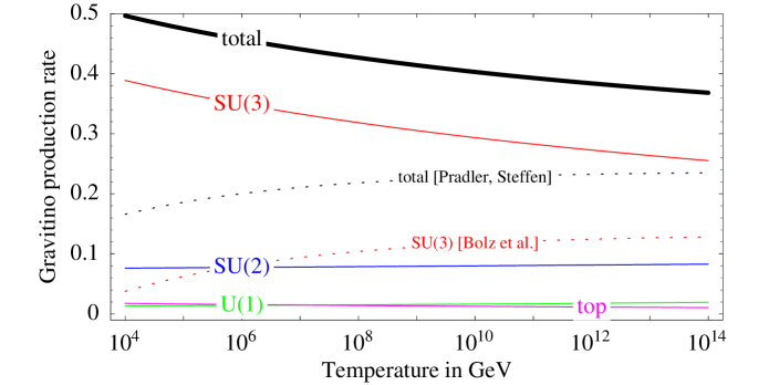
Figure 12: Production rate $\gamma=dN/dV\,dt$ in units of $T^{6}/\bar{M}_{\rm Pl}^{2}$ for the spin-3/2 gravitino components in the MSSM. The upper curve is the total rate, and the other continuous curves show the contributions from $\{g_{3},g_{2},g_{Y},\lambda_{t}\}$ interactions (summed over decay and scattering processes). The production rate for the Goldstino spin-1/2 components is obtained by multiplying these four contributions times $\{M_{3}^{2},M_{2}^{2},M_{1}^{2},A_{t}^{2}\}/3m_{3/2}^{2}$ respectively. The dotted curve show previous results from [Buch] and [postBuch].

7 Conclusions

Previous computations of the thermal gravitino production rate [Buch, postBuch] were performed at leading order in small gauge couplings, finding a rate of the form $\gamma\propto g^{2}\ln 1/g$, which behaves unphysically when extrapolated to the true MSSM values of the gauge couplings, $g\sim 1$ (see fig. 1). We improved on these results in the following ways:

1. We included gravitino production via gluon $\to$ gluino + gravitino and other decays: these effects first arise at higher order in $g$ (the phase space is opened by thermal masses), but are enhanced with respect to scattering processes by a phase-space $\pi^{2}$ factor, typical of 3-body vs 4-body rates. The gravitino production rate becomes about twice larger, or more if $M_{3}\,\raise 1.29167pt\hbox{$>$\kern-7.5pt\lower 4.30554pt\hbox{$\sim$}}\,M_{1,2}\gg m_{3/2}$.

2. We added production processes induced by the top quark Yukawa coupling. This enhances the gravitino production rate by almost $10\%$ or more if $A_{t}$ is bigger than gaugino masses.

3. Finally, we computed the gravitino abundance replacing the instant reheating approximation with the standard definition of the reheating process, where $T_{\rm RH}$ is not the maximal temperature but defines the temperature at which inflaton decay ends, ceasing to release entropy. This improvement decreases the gravitino abundance by $25\%$ and allows a precise comparison with leptogenesis [DI], where reheating was included in [leptog].

Our result for the gravitino production rate is

$$\gamma=\gamma_{D}+\gamma_{S}^{\rm sub}+\gamma_{\rm top}.$$ (7.1)

where the decay rate $\gamma_{D}$ (which dominates the total rate) is given in eq. (4.6), the subtracted scattering rate $\gamma_{S}^{\rm sub}$ in eq. (2.6), and the rate induced by the top Yukawa coupling in eq. (5.2). Fig. 12 summarizes our results, showing the value of the dimensionless combination $\gamma/(T^{6}/\bar{M}_{\rm Pl}^{2})$ (as well as the values of the single gauge and top contributions to it) which determines the gravitino abundance as in  (6.5). In this plot we assumed $\lambda_{t}=0.7$ and a unified $\alpha=1/24$, renormalized at the scale $M_{\rm GUT}=2\cdot 10^{16}\,{\rm GeV}$.

Accessory results scattered through the paper include: a clean precise re-derivation of gravitino couplings; expressions for thermal masses in a generic supersymmetric theory; the observation that they respect supersymmetry at energy much larger than the temperature; a collection of formulæ for thermal corrections to vectors (including correct imaginary parts) beyond the Hard Thermal Loop (HTL) approximation; a possibly non-standard discussion of the physical meaning of negative spectral densities; a technique that allows to deal with Coulomb-like infra-red divergences without introducing an arbitrary splitting scale $k_{*}$ that satisfies the problematic condition $gT\ll k_{*}\ll T$.

A curious result simplified our computation: the differential production rates for the spin 3/2 and for the spin 1/2 (Goldstino) gravitino component are equal up to a universal prefactor, despite that Goldstino couplings (to dimension-1 SUSY-breaking soft terms in the supercurrent) apparently are much simpler than the spin-3/2 couplings (gravitational, to the supersymmetric supercurrent). This equality holds thanks to various cancellations, such that various troubling contributions automatically drop out from our computation.

Acknowledgements

We thank R. Barbieri, C. Scrucca, G. Giudice, A. Notari, G. Moore. A.S. thanks R. Rattazzi who suggested that we look into the higher-order corrections to the gravitino production rate because this problem involves conceptual issues of academic interest. On the contrary the 100% enhancement with respect to previous results is relevant for phenomenology, and we could compute it without understanding why we don’t need to understand how to write the supercurrent at finite temperature.

Appendix A Gravitino propagator and couplings

We here derive the needed gravitino propagator and couplings, both generic and specialized for the MSSM. The results contained in this section are not new, but they are useful for two reasons. First, because all factors ($i,\gamma_{5},P_{L}$, etc) and subtleties should be right, and are relevant for satisfying the consistency checks that we performed in our subsequent computations. Second, because we recomputed relevant gravitino properties in a way that we consider simpler than in previous literature: we proceed directly, without using Noether and supergravity techniques, which are unnecessarily cumbersome for our purposes. We use the standard Weyl spinor and $\gamma$-matrix conventions corresponding to the signature $(+---)$, see e.g. [Lykken]. The phase of the gauginos is chosen such that gaugino couplings to matter are real. We assume a Minkowski background i.e. we neglect the small cosmological constant.

A.1 The gravitino Lagrangian

The gravitino is the gauge field associated with local supersymmetry, and becomes massive by means of a super-Higgs mechanism: ‘eating’ the massless Goldstino fermion arising when global supersymmetry is spontaneously broken. This is analogous to a gauge vector that becomes massive via the usual Higgs mechanism, so that we start recalling some general properties of this well known simpler case, and this analogy will later allow us to derive gravitino properties following the same logic.

Paradigmatic digression

We thus consider a U(1) gauge symmetry broken by the vev of a charged scalar field $H$. In the limit of vanishing gauge coupling, a massless Goldstone $\chi$ appears in the expansion of $H$ around the minimum, $H=v+i\chi$, and $\chi$ transforms (under a U(1) rotation with infinitesimal angle $\varepsilon$) as $\delta\chi=v\varepsilon$. The total U(1) current is given by

$$J_{\mu}=J_{\mu}^{\text{mat}}-v\,\partial_{\mu}\chi,$$ (A.1)

where $J_{\mu}^{\text{mat}}$ is the U(1) current of the rest of the theory (e.g. fermionic matter). The total U(1) current is conserved:

$$\partial_{\mu}J_{\mu}=\partial_{\mu}J_{\mu}^{\text{mat}}-v\,\partial^{2}\chi=0.$$ (A.2)

This is the case if and only if the Lagrangian contains the coupling

$${L}\supset\frac{1}{v}\chi\cdot\partial_{\mu}J_{\mu}^{\text{mat}}.$$ (A.3)

This is sometimes known as Goldberger-Treiman relation, and shows that Goldstone interactions are predicted in terms of nonconservation of the matter symmetry current induced in the process of symmetry breaking.

When the U(1) symmetry is gauged, the total gauge-invariant Lagrangian is

$$\hbox{\smallsfs L}=-\frac{1}{4}F_{\mu\nu}^{2}+\frac{1}{2}(\partial_{\mu}\chi-vA_{\mu})^{2}+(A_{\mu}-\frac{1}{v}\partial_{\mu}\chi)J_{\mu}^{\text{mat}}+\hbox{\smallsfs L}_{\text{mat}}.$$ (A.4)

We can fix the unitary gauge by setting $\chi$ to zero or, equivalently, by redefining $A_{\mu}^{\prime}=A_{\mu}-\partial_{\mu}\chi/v$. The second term in (A.4) becomes a mass term for $A_{\mu}^{\prime}$. Notice that while $A_{\mu}$ couples to the total conserved current $J_{\mu}$ given by eq. (A.1), the massive vector $A_{\mu}^{\prime}$ couples to $J_{\mu}^{\text{mat}}$.

The last thing that we want to recall concerns production of massive gauge bosons at high energy $E\gg v$. The effective Lagrangian appropriate for this situation is obtained from (A.4) by keeping terms with the highest number of derivatives in $A_{\mu}$ and $\chi$, and is given by

$$\hbox{\smallsfs L}_{\text{HE}}=-\frac{1}{4}F_{\mu\nu}^{2}+\frac{1}{2}(\partial_{\mu}\chi)^{2}+A_{\mu}J_{\mu}^{\text{mat}}+\frac{1}{v}\chi\cdot\partial_{\mu}J_{\mu}^{\text{mat}}+{L}_{\text{mat}}.$$ (A.5)

We thus see that the total cross section can be approximated (up to terms suppressed by $v/E$) by the sum of massless gauge boson production plus production of Goldstones with coupling (A.3):

$$\sigma(A_{\mu}^{\prime})=\sigma(A_{\mu})+\sigma(\chi).$$ (A.6)

This statement is called the equivalence theorem. It can also be deduced (in a less transparent way) from the fact that the physical state projector for the gauge boson of mass $m$ takes the form $-g_{\mu\nu}+k_{\mu}k_{\mu}/m^{2}$. Notice that, while to get the correct Goldstone production rate it is crucial to take current nonconservation into account, in computing $\sigma(A_{\mu})$ we can actually assume that $J_{\mu}^{\text{mat}}$ is conserved.

The main points of the above discussion — the form of the total current, the Goldberger-Treiman relation, the fact that the massive gauge boson couples to the same matter current, and the equivalence theorem — will find their analogues in the gravitino case.

Goldstino interaction

We now repeat the steps in the previous section in the case of supersymmetry, under which the Goldstino $\chi$ transforms as $\delta\chi=\sqrt{2}F\varepsilon$, where $F$ is a supersymmetry-breaking vev and $\varepsilon$ is the supersymmetric parameter. The supercurrent is

$$S^{\mu}=S_{\text{vis}}^{\mu}+i\sqrt{2}F\gamma^{\mu}\chi$$ (A.7)

where the apex ‘vis’ signals that we are interested in theories consisting of a visible and a hidden sector. Supersymmetry is broken spontaneously in a heavy hidden sector, and its low energy remnant is the Goldstino field: all other hidden sector fields can be integrated out, if one is interested in energies below the messenger scale. The full supercurrent is conserved:

$$\partial_{\mu}S^{\mu}=\partial_{\mu}S_{\text{vis}}^{\mu}+i\sqrt{2}F\partial\!\!\!\raisebox{2.0pt}[0.0pt][0.0pt]{$\scriptstyle/$}\,\,\chi=0.$$ (A.8)

The vanishing of (A.8) gives the equation of motion for $\chi$, and consequently implies the following Goldstino Lagrangian:

$$\hbox{\smallsfs L}_{\text{Goldstino}}=\frac{1}{2}\bar{\chi}i\partial\!\!\!\raisebox{2.0pt}[0.0pt][0.0pt]{$\scriptstyle/$}\,\,\chi-\frac{1}{\sqrt{2}F}\bar{\chi}\,\partial_{\mu}S_{\text{vis}}^{\mu}+\cdots$$ (A.9)

where $\cdots$ indicates couplings involving two or more Goldstinos, not needed in our computation.

Massless gravitino

In the supersymmetric limit, the massless gravitino is described by a Majorana Rarita-Schwinger field $\psi_{\mu}$ with Lagrangian

$${{L}}=-\frac{1}{2}\varepsilon^{\mu\nu\rho\sigma}\bar{\psi}_{\mu}\gamma_{5}\gamma_{\nu}\partial_{\rho}\psi_{\sigma}$$ (A.10)

invariant under the gauge SUSY transformations with parameter $\varepsilon$: $\delta\psi_{\mu}=-2\bar{M}_{\text{Pl}}\partial_{\mu}\varepsilon$. Here $\bar{M}_{\mathrm{Pl}}=M_{\mathrm{Pl}}/8\pi=2.4~{}10^{18}\,\mathrm{GeV}$ is the reduced Planck mass. The variation of the matter action defines the Majorana supercurrent $S_{\mu}$ as

$$\delta S_{\text{matter}}=\int d^{4}x~{}\bar{S}^{\mu}\partial_{\mu}\varepsilon.$$ (A.11)

Demanding that the full action is invariant to zeroth order in $\bar{M}_{\text{Pl}}^{-1}$ one obtains how the massless gravitino interacts with the supercurrent

$${\hbox{\smallsfs L}}_{\text{int}}=\frac{1}{2\bar{M}_{\mathrm{Pl}}}\bar{\psi}_{\mu}S^{\mu}.$$ (A.12)

Super-Higgs mechanism

We will now follow how the massless gravitino eats the Goldstino, getting a mass via the super-Higgs mechanism. First of all, the gauge-invariant action for the goldstino-gravitino system is [GraviGold, Cremmer]:

$$\hbox{\smallsfs L}=-\frac{1}{2}\varepsilon^{\mu\nu\rho\sigma}\bar{\psi}_{\mu}\gamma_{5}\gamma_{\nu}\partial_{\rho}\psi_{\sigma}+\frac{1}{2}\bar{\chi}i\partial\!\!\!\raisebox{2.0pt}[0.0pt][0.0pt]{$\scriptstyle/$}\,\,\chi-m_{3/2}\bigg{[}\frac{1}{4}\bar{\psi}_{\mu}[\gamma^{\mu},\gamma^{\nu}]\psi_{\nu}+\bar{\chi}\chi-\sqrt{\frac{3}{2}}\bar{\psi}_{\mu}i\gamma^{\mu}\chi\bigg{]}.$$ (A.13)

It contains a gravitino-goldstino mixing mass term, that agrees with the form of the supercurrent, eq. (A.7). Indeed, this Lagrangian is invariant under the local field transformations:

$$\delta\psi_{\mu} =-\bar{M}_{\text{Pl}}(2\partial_{\mu}\varepsilon+im_{3/2}\gamma^{\mu}\varepsilon),$$

$$\delta\chi =\sqrt{2}F\varepsilon,$$

provided that the gravitino mass $m_{3/2}$ and the SUSY breaking vev $F$ are related as

$$m_{3/2}=\frac{F}{\sqrt{3}\bar{M}_{\text{Pl}}}.$$ (A.14)

(The derivation above used the flat space assumption). Introducing the gravitino mass required a deformation of the supersymmetric transformation of the gravitino, and the gravitino interaction term with matter (A.12) is no longer invariant. To restore invariance, we must add to the Lagrangian the term

$$\frac{m_{3/2}}{2\sqrt{2}F}\bar{\chi}i\not{S}=\frac{1}{2\bar{M}_{\text{Pl}}}\frac{1}{\sqrt{6}}\bar{\chi}i\not{S}\qquad\not{S}=\gamma_{\mu}S_{\mathrm{vis}}^{\mu}$$ (A.15)

It may seem surprising at first to find this new coupling of Goldstino to the supercurrent in addition to the one in (A.9). However, there is no contradiction since the new term vanishes as gravity is decoupled.

We can now choose the unitary gauge $\chi=0$ or equivalently define

$$\Psi_{\mu}=\psi_{\mu}-\frac{1}{\sqrt{6}}i\gamma^{\mu}\chi-\sqrt{\frac{2}{3}}\frac{\partial_{\mu}\chi}{m_{3/2}},$$ (A.16)

such that the whole Lagrangian describing gravitino, goldstino, and their interaction with matter can be rewritten as [Cremmer]

$$\hbox{\smallsfs L}=-\frac{1}{2}\varepsilon^{\mu\nu\rho\sigma}\bar{\Psi}_{\mu}\gamma_{5}\gamma_{\nu}\partial_{\rho}\Psi_{\sigma}-\frac{m_{3/2}}{4}\bar{\Psi}_{\mu}[\gamma^{\mu},\gamma^{\nu}]\Psi_{\nu}+\frac{1}{2\bar{M}_{\mathrm{Pl}}}\bar{\Psi}_{\mu}S_{\mathrm{vis}}^{\mu}.$$ (A.17)

This is the Lagrangian describing the massive gravitino $\Psi_{\mu}$. We see that it couples to $S_{\mathrm{vis}}^{\mu}$.

Equivalence theorem

The Lagrangian (A.17) could be used to study production of massive gravitinos at any energy below the messenger scale. In this paper, we are interested in energies much bigger than $m_{3/2}$ and the sparticle masses. A simpler effective Lagrangian appropriate for these energies can be derived by noticing that the mass terms and mixings between $\psi_{\mu}$ and $\chi$ in (A.13) can be neglected. Thus we can study production of massless gravitinos $\psi_{\mu}$ and Goldstinos $\chi$ coupled to the visible sector by

$$\hbox{\smallsfs L}_{\text{int}}=\frac{1}{2\bar{M}_{\text{Pl}}}\bar{S}_{\text{vis}}^{\mu}(\psi_{\mu}-\sqrt{\frac{1}{6}}i\gamma_{\mu}\chi)+\frac{1}{\sqrt{2}F}\bar{\chi}\partial_{\mu}S_{\text{vis}}^{\mu}.$$ (A.18)

This is the analogue of the previously mentioned equivalence theorem for production of gauge bosons at energies much larger than their masses. In the massive gauge boson case, the equivalence theorem could also be derived from the form of the physical state projector of the massive gauge boson. Below we will see that an analogous derivation can also be given for the massive gravitino case. Just as in the gauge boson case, we can assume that the supercurrent in the coupling $\bar{S}_{\text{vis}}^{\mu}\psi_{\mu}$ is conserved; in the Goldstino coupling the current nonconservation is of course crucial and has to be taken into account.

A further simplification concerns the Goldstino coupling (A.15): as we explain below this coupling is irrelevant in MSSM at energies much above the $\mu$-term due to approximate scale-invariance. Thus

$$\hbox{\smallsfs L}_{\text{int}}=\frac{1}{2\bar{M}_{\text{Pl}}}\bar{\psi}_{\mu}S_{\text{vis}}^{\mu}+\frac{1}{\sqrt{2}F}\bar{\chi}\partial_{\mu}S_{\text{vis}}^{\mu}\qquad\text{ \ (MSSM)}.$$ (A.19)

It is instructive to compare the relative importance of the two terms in (A.19) for the total production rate. Since the divergence of the supercurrent will be proportional to the soft-breaking masses (see below), the effective coupling in the second term is $m_{\text{soft}}/F\sim 1/M_{\text{mess}}$. Thus the two terms are equally important if SUSY breaking is mediated by gravity, $M_{\mathrm{mess}}\sim\bar{M}_{\mathrm{Pl}}$. If instead $M_{\mathrm{mess}}\ll\bar{M}_{\mathrm{Pl}}$, like in gauge-mediation models, the Goldstino term dominates [gravitinoCosmo].

A.2 The gravitino propagator and polarization tensor

Massless gravitino

Since the Lagrangian is invariant under local supersymmetry, the same physics can be described by different choices of gravitino propagators and polarization tensors. Analogously to the vector case, the sum over the two physical transverse polarizations is (see [Van])

$$\Pi^{3/2}_{\mu\nu}(P)\equiv\sum_{i=\pm}\Psi_{\mu}^{(i)}\bar{\Psi}_{\nu}^{(i)}=\frac{1}{2}\gamma_{\nu}P/\,\gamma_{\mu}-\frac{1}{2}P_{\mu}\gamma_{\nu}P/\,\not{Q}-\frac{1}{2}P_{\nu}\not{Q}P/\gamma^{\mu}+P_{\mu}P_{\nu}\not{Q}$$ (A.20)

where $U$ is an arbitrary 4-velocity that defines a preferred reference frame used to define what ‘transverse’ means, and $Q^{\mu}\equiv[2U^{\mu}(U\cdot P)-P^{\mu}]/2(U\cdot P)^{2}$. Gauge-invariant observables do not depend on the choice of $U$.

As usual, local gauge invariance allows to define more convenient gauge choices. For example, one can impose the gauge-fixing condition $F\equiv\gamma^{\mu}\Psi_{\mu}=0$ (in this gauge one also has $\partial_{\mu}\Psi^{\mu}=0$ as a consequence of the equations of motion). To derive the propagator, it is best to consider an analogue of the $\xi$-gauge by adding to the Lagrangian the gauge-fixing term $\bar{F}i\partial\!\!\!\raisebox{2.0pt}[0.0pt][0.0pt]{$\scriptstyle/$}\,\,F/\xi$. Then the kinetic operator is invertible, and the gravitino propagator is [Das]

$$\frac{\Pi^{3/2}_{\mu\nu}}{P^{2}+i\varepsilon}\qquad\hbox{with}\qquad\Pi^{3/2}_{\mu\nu}=\frac{1}{2}\gamma^{\nu}P/\,\gamma^{\mu}-(2+\xi)\frac{P^{\mu}P/\,\,P^{\nu}}{P^{2}}.$$ (A.21)

As usual, $\Pi^{3/2}_{\mu\nu}$ is also the projector to be used when the massless gravitino production rate is summed over the gravitino polarizations. The dependence on the gauge-fixing parameter $\xi$ is irrelevant because the massless gravitino couples to the conserved supercurrent, $P_{\mu}S_{\mu}=0$. For the simplest choice $\xi=-2$ one has

$$\Pi^{3/2}_{\mu\nu}=\frac{1}{2}\gamma_{\nu}P/\,\gamma_{\mu}=-\frac{1}{2}\gamma_{\mu}P/\,\gamma_{\nu}-P/\,\eta_{\mu\nu}+\gamma_{\mu}P_{\nu}+P_{\mu}\gamma_{\nu}.$$ (A.22)

The last two terms do not contribute, again because the supercurrent is conserved. For our later computation we will choose

$$\Pi^{3/2}_{\mu\nu}=-\frac{1}{2}\gamma_{\mu}P/\,\gamma_{\nu}-P/\,\eta_{\mu\nu}.$$ (A.23)

Massive gravitino and the equivalence theorem

The massive gravitino is described by the Lagrangian (A.17). The mass term breaks the gauge symmetry present in the massless case. The equations of motion coming from the free part of (A.17) imply

$$\gamma_{\mu}\Psi_{\mu}=0,\qquad\partial_{\mu}\Psi_{\mu}=0,\qquad(\not{P}-m_{3/2})\Psi_{\mu}=0.$$ (A.24)

In the massless case the first two equations could have been imposed as gauge-fixing conditions. The resulting propagator is [Van] $\Pi_{\mu\nu}/(P^{2}-m_{3/2}^{2}+i\varepsilon)$ where

$$\Pi_{\mu\nu}=-(\not{P}+m_{3/2})\left(g_{\mu\nu}-\frac{P_{\mu}P_{\nu}}{m_{3/2}^{2}}\right)-\frac{1}{3}\left(\gamma^{\mu}+\frac{P^{\mu}}{m_{3/2}}\right)(\not{P}-m_{3/2})\left(\gamma^{\nu}+\frac{P^{\nu}}{m_{3/2}}\right).$$ (A.25)

Again $\Pi_{\mu\nu}$ is also the polarization tensor to be used when summing over all physical polarizations: $\Pi_{\mu\nu}=\sum_{i=\pm\frac{1}{2},\pm\frac{3}{2}}\Psi_{\mu}^{(i)}\bar{\Psi}_{\nu}^{(i)}$. One can check that (A.25) is consistent with (A.24).

In this paper we are interested in production of ultrarelativistic gravitinos. To study this limit, we expand (A.25) in powers of $m_{\text{3/2}}$:

$$\Pi_{\mu\nu}= ~{}\frac{2}{3}\frac{P_{\mu}P_{\nu}\not{P}}{m_{3/2}^{2}}+\frac{4P_{\mu}P_{\nu}-\not{P}\gamma^{\nu}P^{\mu}-\gamma^{\mu}\not{P}P^{\nu}}{3m_{3/2}}$$

$$~{}+\left(-g_{\mu\nu}\not{P}-\frac{1}{3}\gamma_{\mu}\not{P}\gamma_{\nu}+\frac{1}{3}\gamma^{\mu}P^{\nu}+\frac{1}{3}\gamma^{\nu}P^{\mu}\right)+\left(\frac{\gamma^{\mu}\gamma^{\nu}}{3}-g^{\mu\nu}\right)m_{3/2}.$$ (A.26)

If the supercurrent to which the gravitino couples is conserved, the terms singular in $m_{3/2}$ give no contribution. The last term vanishes for $m_{3/2}\rightarrow 0$. The term that does not depend on $m_{3/2}$ differs from the massless gravitino projector (A.22) by $\gamma_{\mu}\not{P}\gamma_{\nu}/6$, modulo irrelevant terms proportional to $P_{\mu}$ or $P_{\nu}$.

Thus in the limit $m_{3/2}\rightarrow 0$ we not only recover the massless gravitino, but also get an additional massless spin $1/2$ fermion which couples to ${1}/\sqrt{6}$ times the ‘trace’ of the supercurrent, $\not{S}=\gamma_{\mu}S^{\mu}$. This is akin to the van Dam-Veltman-Zakharov discontinuity [vVZ] encountered when adding to the graviton a Fierz-Pauli mass term $m_{g}$: the limit $m_{g}\rightarrow 0$ then describes the usual massless graviton plus a scalar coupled to the trace of the energy-momentum tensor $T_{~{}\mu}^{\mu}$. In our case this ‘discontinuity’ is entirely expected and is consistent with the equivalence theorem as expressed by eq. (A.18): the extra spin 1/2 fermion is nothing but the Goldstino.

When we take soft SUSY-breaking into account, the supercurrent is no longer conserved. The first term in (A.26) can then be interpreted as corresponding to the Goldstino production due to the last term in (A.18) (the coefficient agrees as one checks using (A.14)). In this derivation of the equivalence theorem it is non-obvious that the terms in (A.25) proportional to $m_{3/2}^{-1}$ should cancel, as is required for full agreement with (A.18). However this cancellation does happen, as verified in the explicit computations needed for this paper.

A.3 MSSM supercurrent at zero temperature

Gravitino couplings

In a generic renormalizable SUSY gauge theory with vector supermultiplets $(A_{\mu}^{a},\lambda^{a})$ and matter chiral supermultiplets $\Phi_{i}=(\phi_{i},\xi_{i})$ and superpotential $W$ the Weyl part $s^{\mu}$ of the Majorana supercurrent $S^{\mu}=(s^{\mu}$,$\bar{s}^{\mu})$ is (see e.g. [Drees] or explicitly compute it)

$$s^{\mu}=-\sqrt{2}\left[(D^{\nu}\phi_{i})^{\ast}(\sigma_{\nu}\bar{\sigma}^{\mu}\xi_{i})+iW_{i}^{\ast}(\phi^{\ast})\sigma^{\mu}\bar{\xi}_{i}\right]-\frac{1}{2}F_{\nu\rho}^{a}(\sigma^{\nu}\bar{\sigma}^{\rho}\sigma^{\mu}\bar{\lambda}^{a})-ig(\phi_{i}^{\ast}T_{ij}^{a}\phi_{j})(\sigma^{\mu}\bar{\lambda}^{a})$$ (A.27)

where $D_{ij}^{\mu}=\delta_{ij}\partial_{\mu}+igA^{\mu a}T_{ij}^{a}$ is the gauge-covariant derivative. The first two terms are the supercurrent of the Wess-Zumino model and of the SUSY gauge theory without matter. The third term is a correction which arises as a result of coupling between the two. (With the Noether formalism it would arise because the Lagrangian is supersymmetric up to a total derivative). In 4-component notation it becomes:

$$S^{\mu}= -\sqrt{2}\left[(D^{\nu}\phi_{i})^{\ast}(\gamma^{\nu}\gamma^{\mu}\xi_{L}^{i})+(D^{\nu}\phi_{i})(\gamma^{\nu}\gamma^{\mu}\xi_{R}^{i})-iW_{i}(\phi)\gamma^{\mu}\xi_{L}^{i}-iW_{i}^{\ast}(\phi^{\ast})\gamma^{\mu}\xi_{R}^{i}\right]$$ (A.28)

$$-\frac{1}{4}F_{\nu\rho}^{a}[\gamma^{\nu},\gamma^{\rho}]\gamma^{\mu}\gamma^{5}\lambda^{a}-ig(\phi_{i}^{\ast}T_{ij}^{a}\phi_{j})\gamma^{\mu}\lambda^{a}$$

where we introduced Majorana spinors ($\xi_{i},\bar{\xi}_{i})^{T}$ and $(\lambda^{a},\bar{\lambda}^{a})^{T}$ which by abuse of notation we denoted again $\xi_{i}$ and $\lambda^{a}$. As usual $\xi_{L}\equiv P_{L}\xi$, $\xi_{R}\equiv P_{R}\xi$, $W_{i}=\partial W/\partial\phi_{i}$ and the index $i$ runs over all chiral multiplets.

The supercurrent is conserved $\partial_{\mu}S^{\mu}=0$ as a consequence of equations of motion. After fixing the vector gauge symmetries in the usual way, the vector equations of motion change due to the gauge-fixing terms and to the ghost current. The ghosts are scalars under supersymmetry (in particular, they do not have superpartners and they couple only to the gauge field but not to the gaugino), and one could be worried that SUSY is broken by the gauge choice. Indeed the supercurrent divergence is no longer zero, however it is BRST exact (see e.g. [BRST]). Thus the amplitude for longitudinal gravitino emission still vanishes, and the gravitino gauge invariance is preserved.

The terms proportional to $\gamma^{\mu}$ are sometimes omitted from the supercurrent expression (A.28), because they do not contribute to the massive gravitino production due to the on-shell condition $\gamma^{\mu}\Psi_{\mu}=0$. However, one should be careful to keep these terms if one wants to use the equivalence theorem and the massless gravitino gauge invariance, because the supercurrent is no longer conserved if they are omitted.

Goldstino couplings

According to the equivalence theorem discussed above, the spin $\pm 1/2$ component of the massive gravitino at high energies can be replaced by the Goldstino coupled to the divergence and trace $\not{S}$ of the visible sector supercurrent with coefficients given in (A.18). The divergence $\partial_{\mu}S_{\text{vis}}^{\mu}$ measures the SUSY breaking in the visible sector, which at energies lower than the messenger scale looks like explicit breaking by soft terms. In absence of soft terms $\partial_{\mu}S_{\text{vis}}^{\mu}=0$ as a consequence of equations of motion. Nonzero soft terms modify the equations of motion, so that $\partial_{\mu}S_{\text{vis}}^{\mu}\sim m_{\text{soft}}\neq 0$. For dimensional reasons we can neglect dimension 2 soft terms (i.e. scalar squared masses): only soft terms with dimension 1 (i.e. gaugino masses $M$ and trilinear scalar couplings $A$) contribute to Goldstino production at dominant order, $\gamma\propto T^{6}$. By taking into account how the relevant soft terms modify the equations of motion of particles and sparticles we get

$$\partial_{\mu}S_{\text{vis}}^{\mu}=-\frac{iM}{4}F_{\nu\rho}^{a}[\gamma^{\nu},\gamma^{\rho}]\gamma^{5}\lambda^{a}-Mg(\phi^{\ast}T^{a}\phi)\lambda^{a}+\sqrt{2}[(AW)_{i}(\phi)\xi_{L}^{i}+(AW)_{i}^{\ast}(\phi^{\ast})\xi_{R}^{i}]$$ (A.29)

where $i$ runs over all chiral multiplets and a sum is understood over the components of the gauge group. The presence of the second gauge term was first noticed in [LeeWu], and is here reobtained via a simple direct computation. Notice that to get it, it is crucial to keep the last term in eq. (A.28), that does not contribute to massive gravitino production due to the on-shell condition $\gamma^{\mu}\Psi_{\mu}=0$.

In the MSSM the relevant soft terms are the three gaugino masses $M_{1,2,3}$ and the top $A$-term, $A_{t}$:

$$\hbox{\smallsfs L}_{\text{soft}}=\sum_{N=1}^{3}\frac{M_{N}}{2}\lambda^{a}_{N}\lambda^{a}_{N}+\lambda_{t}A_{t}(\tilde{Q}\tilde{U}H_{\mathrm{u}}+\hbox{h.c.})+\cdots.$$ (A.30)

Finally, we elaborate on the Goldstino coupling to $\not{S}$, finding that it can be neglected in the MSSM. Using $\gamma^{\mu}[\gamma^{\nu},\gamma^{\rho}]\gamma^{\mu}=0$, (A.27) implies

$$\bar{\sigma}^{\mu}s^{\mu}=-\sqrt{2}\left[-2(D^{\nu}\phi_{i})^{\ast}\sigma_{\nu}\xi_{i}+4iW_{i}^{\ast}(\phi^{\ast})\bar{\xi}_{i}\right]-4ig(\phi_{i}^{\ast}T_{ij}^{a}\phi_{j})\bar{\lambda}^{a}$$ (A.31)

Rewriting the first term as

$$(D^{\nu}\phi_{i})^{\ast}\sigma_{\nu}\xi_{i}=\partial_{\nu}(\phi_{i}^{\ast}\sigma_{\nu}\xi_{i})-\phi_{i}^{\ast}\sigma_{\nu}D_{\nu}\xi_{i}$$

and using the fermion equation of motion, several terms cancel and we remain with

$$\bar{\sigma}^{\mu}s^{\mu}=2\sqrt{2}\partial_{\nu}(\phi_{i}^{\ast}\sigma_{\nu}\xi_{i})+2\sqrt{2}i[\phi_{i}^{\ast}W_{ij}^{\ast}-2W_{j}^{\ast}(\phi^{\ast})]\bar{\xi}_{j}$$ (A.32)

The first term does not contribute to massless Goldstino production rate since $\bar{\chi}\partial_{\nu}(\phi_{i}^{\ast}\sigma_{\nu}\xi_{i})$ vanishes on-shell due to $\bar{\sigma}_{\nu}\partial_{\nu}\chi=0.$ The second term vanishes if $W_{j}$ is a quadratic function of the fields, i.e. for cubic terms in $W$. We thus conclude that the only nontrivial coupling to Goldstino arising from the (A.15) vertex is due to the $\mu$-term and is of the form

$$\sim\frac{\mu}{\bar{M}_{\text{Pl}}}\chi(H_{1}\tilde{H}_{2}+\tilde{H}_{1}H_{2})+\text{h.c.}$$

This vertex is irrelevant at energies much bigger than $\mu$.

The reason for the above is that the trace of the supercurent $\not{S}$ falls into a supersymmetric “anomaly multiplet”

$$\{\not{S},\partial_{\mu}R^{\mu},T_{\,\mu}^{\mu}\},$$

where $T_{\,\mu}^{\mu}$ is the trace of the energy-momentum tensor expressing the scale invariance of the theory, and $R^{\mu}$ is the current of the $R$-symmetry under which all chiral multiplets have charge $2/3$ (see [Weinberg]). In MSSM, both the scale invariance and the above $R$-symmetry are broken classically only by the $\mu$-term, and this explains $\not{S}\sim\mu$. At quantum level the scale invariance and the $R$-symmetry are anomalous, e.g. $\partial_{\mu}R^{\mu}$ is given by the triangle anomaly equation:

$$\partial_{\mu}R^{\mu}=\sum\frac{b_{N}g_{N}^{2}}{48\pi^{2}}F_{\mu\nu}^{(N)}\tilde{F}_{\mu\nu}^{(N)}$$

where the anomaly coefficients $b_{N}=\{11,1,-3\}$ are the same as the one-loop $\beta$-function coefficients of the MSSM gauge groups, which is again related to the fact that $\partial_{\mu}R^{\mu}$ and $T_{\,\mu}^{\mu}$ are in the same supermultiplet. Since supersymmetry relates $\not{S}$ to $\partial_{\mu}R^{\mu}$, one can show that (see [West])

$$\not{S}=\sum\frac{b_{N}g_{N}^{2}}{16\pi^{2}}F_{\mu\nu}^{(N)}[\gamma^{\mu},\gamma^{\nu}]\lambda^{(N)}.$$ (A.33)

Below we argue that this equation can be used also at finite temperature.

A.4 Gravitino and goldstino couplings at finite temperature

Gravitino production from a supersymmetric thermal plasma is best studied in terms of its non-time ordered propagator $\Pi^{<}(P)$ given by eq. (2.2). Supersymmetry is broken by finite temperature, but this breaking is spontaneous, so the supercurrent remains conserved: $\partial_{\mu}{}S_{\mu}=0$ holds as an operator equation. This means that the production rate of longitudinal gravitinos vanishes also at finite temperature. Equivalently, $\Pi^{<}(P)$ is invariant under gauge transformations of the gravitino polarization tensor, $\delta\Pi_{\mu\nu}^{3/2}=P_{\mu}A_{\nu}+P_{\nu}B_{\mu}$, with arbitrary $A,B$. The statements of the previous paragraph should hold identically in any computation including all diagrams to a given order in the thermal bath coupling $g$. In practice, however, it may be difficult to see the vanishing of $\delta\Pi^{<}$ explicitly. E.g. as explained in section 2 we are resumming a well-defined class of physical effects to order $g^{4}$: those enhanced by a $1\to 2$ phase space factor, unlike a generic ${\cal O}(g^{4})$ correction. More precisely, diagram D is computed including thermal corrections to the propagators of particles to which the gravitino couples, while diagrams S${}_{1,2,3}$ are computed using tree-level propagators. In particular, we do not include corrections to the gravitino vertex. For this reason we expect a residual gravitino gauge dependence, which we believe to be of relative order $g^{2}/\pi^{2}$ with respect to our result. The reason is that in our calculation of the massless gravitino production rate, thermal masses act similar to soft SUSY-breaking terms, modifying equations of motion by terms of order $g^{2}T$, so that $\partial\cdot S\sim g^{2}T$ rather than being zero. This means that $\delta\Pi^{<}\sim{\cal O}(g^{4})$. We see that this non-gauge invariance is of the right order of magnitude to be cancelled by vertex corrections. The above residual non-gauge invariance can be tolerated when computing the massless gravitino production rate.

When computing the Goldstino production rate, we have taken into account that, in absence of soft-SUSY breaking, the Goldstino coupling to $\partial\cdot S$ vanishes at finite temperature by evaluating the divergence of the supercurrent before computing the thermal matrix element, i.e. we start the finite-temperature computation from eq. (A.29). Since we do not evaluate vertex corrections, this procedure is expected to give a result with the same ${\cal O}(g^{2}/\pi^{2})$ error as the gravitino production rate.

Finally, the anomaly relation (A.33) valid at zero temperature also holds at finite temperature. The argument is the same as in case of the supercurrent conservation: the thermal bath is a background, and (A.33) is a dynamical property of the Hamiltonian valid for any background. In practice this means that the Goldstino coupling to $\not{S}$ can be neglected.

Appendix B Vector propagator at finite temperature

We list the full one-loop expressions for thermal corrections to a vector with four-momentum $K=(\omega,\vec{k})$ ($K^{2}=\omega^{2}-k^{2}$) with respect to the rest frame of the thermal plasma. In general, we denote by $U_{\mu}$ the four-velocity $U_{\mu}$ of the plasma. We use the Feynman gauge where all effects are condensed in two form factors even in the non-abelian case [WeldonVector]. Polarizations are conveniently decomposed in $T$ransverse (i.e. orthogonal to $K$ and to $\vec{k}$), $L$ongitudinal (i.e. orthogonal to $K$ and parallel to $\vec{k}$) and parallel to $K$. The corresponding projectors $(\Pi^{T}+\Pi^{L}+\Pi^{K})_{\mu\nu}=-\eta_{\mu\nu}$ are

$$\halign to=0.0pt{\@eqnsel\hskip\@centering$\displaystyle{#}$&\global\@eqcnt\@ne\hskip 2\arraycolsep\hfil${#}$\hfil& \global\@eqcnt\tw@\hskip 2\arraycolsep$\displaystyle{#}$\hfil&\llap{#}\cr 0.0pt plus 1000.0pt$\displaystyle{\Pi_{\mu\nu}^{T} &10.0pt\hfil${=&10.0pt$\displaystyle{-\tilde{\eta}_{\mu\nu}+\frac{\tilde{K}_{\mu}\tilde{K}_{\nu}}{-k^{2}}= \begin{pmatrix}0 &0\cr 0 &\delta_{ij}- k_{i} k_{j}/k^{2} \end{pmatrix},\\ \Pi_{\mu\nu}^{L} &\hbox to0.0pt{\hss=&-\eta_{\mu\nu}+\frac{K_{\mu}K_{\nu}}{K^{2}}-\Pi_{\mu\nu}^{T},\\\Pi_{\mu\nu}^{K}&=&-\frac{K_{\mu}K_{\nu}}{K^{2}},&(B.1)\cr}}}}}$$

where $\tilde{\eta}_{\mu\nu}=\eta_{\mu\nu}-U_{\mu}U_{\nu}$, $\tilde{K}_{\mu}=K_{\mu}-(K\cdot U)U_{\mu}$. The vector propagator is

$${}^{*}D_{\mu\nu}=i\bigg{[}\frac{\Pi_{\mu\nu}^{T}}{K^{2}-\pi_{0}-\pi_{T}}+\frac{\Pi_{\mu\nu}^{L}}{K^{2}-\pi_{0}-\pi_{L}}+\frac{\Pi_{\mu\nu}^{K}}{K^{2}}\bigg{]}.$$ (B.2)

In the following $\simeq$ denotes the HTL limit, where the result can be expressed in terms of the vector thermal mass $m_{V}^{2}=\frac{1}{6}g^{2}T^{2}(N+N_{S}+N_{F}/2)$, where the $V$ector, $F$ermion and $S$calar coefficients are defined having in mind a group ${\rm SU}(N)$ with $N_{F}$ massless Dirac fermions and $N_{S}$ scalars plus anti-scalars in the fundamental representation. Table 2 lists the explicit values of $N,N_{F},N_{S}$ in the SM and in the MSSM. The one-loop quantum correction at $T=0$ in the $\overline{\rm MS}$ scheme is

$$\begin{array}{cccccccccccccccccccc}\text{π}{}_{\text{0}}\hfill & \text{=}& \hfill & \text{=}\hfill & \text{-}\frac{\text{K}{}^{\text{2}}}{\text{k}{}^{\text{2}}}\text{g}{}^{\text{2}}\text{(N}{}_{\text{S}}\text{H}{}_{\text{S}}\text{+ N}{}_{\text{F}}\text{H}{}_{\text{F}}\text{+ N H}{}_{\text{V}}\text{) ≃-}\frac{\text{K}{}^{\text{2}}}{\text{k}{}^{\text{2}}}\text{(L+1) m}{}_{\text{V}}{}^{\text{2}}\text{,}\text{π}{}_{\text{T}}& \text{=}& \text{-}\frac{\text{π}{}_{\text{L}}}{\text{2}}\text{+ }\frac{\text{g}{}^{\text{2}}}{\text{2}}\text{(N}{}_{\text{S}}\text{G}{}_{\text{S}}\text{+ N}{}_{\text{F}}\text{G}{}_{\text{F}}\text{+ N G}{}_{\text{V}}\text{)≃m}{}_{\text{V}}{}^{\text{2}}\text{(1+}\frac{\text{K}{}^{\text{2}}}{\text{k}{}^{\text{2}}}\frac{\text{L+1}}{\text{2}}\text{)}\text{<span id="A2.Ex37.m1.1.1.1.7.1.21.1.2.1nest" class="ltx\_inline-block ltx\_parbox ltx\_align\_middle" style="width:483.7pt;"> <span id="A2.Ex37.m1.1.1.1.7.1.21.1.2.1.1nest" class="ltx\_p">where</span> </span>}\text{[-2ex] G}{}_{\text{S}}& \text{=}& \text{∫}{}_{\text{0}}{}^{\text{∞}}\frac{\text{dp}}{\text{2}\text{π}{}^{\text{2}}}\text{[}\text{4p - }\frac{\text{K}{}^{\text{2}}}{\text{4k}}\text{L}{}_{\text{-}}\text{]}\text{ n}{}_{\text{B}}\text{(p)≃}\frac{\text{T}{}^{\text{2}}}{\text{3}}\text{G}{}_{\text{F}}& \text{=}& \text{∫}{}_{\text{0}}{}^{\text{∞}}\frac{\text{dp}}{\text{2}\text{π}{}^{\text{2}}}\text{[}\text{4p + }\frac{\text{K}{}^{\text{2}}}{\text{2k}}\text{L}{}_{\text{-}}\text{]}\text{ n}{}_{\text{F}}\text{(p) ≃}\frac{\text{T}{}^{\text{2}}}{\text{6}}\text{G}{}_{\text{V}}& \text{=}& \text{∫}{}_{\text{0}}{}^{\text{∞}}\frac{\text{dp}}{\text{2}\text{π}{}^{\text{2}}}\text{[}\text{4p+}\frac{\text{5K}{}^{\text{2}}}{\text{4k}}\text{L}{}_{\text{-}}\text{]}\text{n}{}_{\text{B}}\text{(p) ≃}\frac{\text{1}}{\text{3}}\text{T}{}^{\text{2}}\text{H}{}_{\text{S}}& \text{=}& \text{∫}{}_{\text{0}}{}^{\text{∞}}\frac{\text{dp}}{\text{2}\text{π}{}^{\text{2}}}\text{[}\text{2p L +}\frac{\text{M}}{\text{k}}\text{+}\frac{\text{k}}{\text{4}}\text{L}{}_{\text{-}}\text{]}\text{n}{}_{\text{B}}\text{(p) ≃}\frac{\text{L+1}}{\text{6}}\text{T}{}^{\text{2}}\text{H}{}_{\text{F}}& \text{=}& \text{∫}{}_{\text{0}}{}^{\text{∞}}\frac{\text{dp}}{\text{2}\text{π}{}^{\text{2}}}\text{[}\text{2pL+}\frac{\text{M}}{\text{k}}\text{]}\text{ n}{}_{\text{F}}\text{(p)≃}\frac{\text{L+1}}{\text{12}}\text{T}{}^{\text{2}}\text{H}{}_{\text{V}}& \text{=}& \text{∫}{}_{\text{0}}{}^{\text{∞}}\frac{\text{dp}}{\text{2}\text{π}{}^{\text{2}}}\text{[}\text{ 2pL+}\frac{\text{M}}{\text{k}}\text{-}\frac{\text{k}}{\text{4}}\text{L}{}_{\text{-}}\text{]}\text{n}{}_{\text{B}}\text{(p) ≃}\frac{\text{L+1}}{\text{6}}\text{T}{}^{\text{2}}& \text{(B.3)}\end{array}havingdefined\text{ω}\text{\_±≡(}\text{ω}\text{±k)/2},L\equiv 1-\frac{\omega }{k}\ln \frac{\omega {}_{+}}{\omega {}_{-}},L{}_{\pm }\equiv \ln \frac{p+\omega {}_{+}}{p+\omega {}_{-}}\pm \ln \frac{p-\omega {}_{+}}{p-\omega {}_{-}},M\equiv (p+\omega {}_{+})(p+\omega {}_{-})\ln \frac{p+\omega {}_{+}}{p+\omega {}_{-}}-(p-\omega {}_{+})(p-\omega {}_{-})\ln \frac{p-\omega {}_{+}}{p-\omega {}_{-}}\simeq 2kpSee\text{<cite class="ltx\_cite ltx\_citemacro\_cite"><span id="A2.Ex37.m1.1.79.1.1nest" class="ltx\_text" style="font-size:90\%;color:\#000000;">[</span><span class="ltx\_ref ltx\_missing\_citation ltx\_ref\_self">WeldonVector</span>, <span class="ltx\_ref ltx\_missing\_citation ltx\_ref\_self">thoma</span><span id="A2.Ex37.m1.1.79.2.2nest" class="ltx\_text" style="font-size:90\%;color:\#000000;">]</span></cite>}forpreviousresults.Weaddedscalarloopsandwrotelogarithmssuchthatimaginaryparts\left(neededtogetspectraldensities\right)areobtainedusingtheprescription\text{ω}\text{→}\text{ω}\text{+ i0^+},with\text{lnz}havingacutalongthenegativerealaxis.Weemphasizethatourexpressionscannotbesimplifiedusing\text{ln(a b) = lna + lnb},becausethiswouldgivewrongimaginaryparts.Thespectraldensitiesemployedineq.\left(\text{<a href="\#S3.Ex10" title="3.3 Vector and gaugino propagators ‣ 3 Finite temperature effects" class="ltx\_ref" style="font-size:90\%;color:\#000000;"><span class="ltx\_text ltx\_ref\_tag">3.3</span></a>}\right)aredefinedas\text{(B.4)Equation B.4B.4ρT=-2Im1K2-π0-πT,ρL=-2ImK2k21K2-π0-πL.}Aswellknown\text{<cite class="ltx\_cite ltx\_citemacro\_cite"><span id="A2.Ex37.m1.1.415.1.1nest" class="ltx\_text" style="font-size:90\%;color:\#000000;">[</span><span class="ltx\_ref ltx\_missing\_citation ltx\_ref\_self">WeldonVector</span>, <span class="ltx\_ref ltx\_missing\_citation ltx\_ref\_self">LeBellac</span><span id="A2.Ex37.m1.1.415.2.2nest" class="ltx\_text" style="font-size:90\%;color:\#000000;">]</span></cite>}\text{ρ}\text{\_L}containsacollectivelongitudinalexcitation,thatcorrespondstolongitudinalwavesofelectricfieldsallowedbyMaxwellequationswithvanishingdielectricconstant.\text{Table 2Table 22Table 2Standard ModelMSSMVectorNNFNSNNFNSGluon SU(3)c360396Weak SU(2)L261/2297Hypercharge U(1)Y0101/2011112Numericalcoefficients}$$