Isospin Chemical potential and temperature effects in the Linear Sigma Model

Abstract

In this letter we explore the temperature and isospin chemical potential ($\mu_{I}$) dependence of the vacuum structure and the meson masses in the linear sigma model, at the one loop level. The sigma meson mass grows steadily with temperature. This behavior does not agree with previous mean field calculations. For the pion our results show the same behavior as the mean field approach. The stability of the vacuum has a very soft dependence on $\mu_{I}$ since this is a second order effect in the tadpole diagrams.

I Introduction

In this letter we address, once again, the question of how the temperature (T) and the chemical potential, in our case isospin chemical potential ($\mu_{I}$), affect the behavior of the linear sigma model. The question is interesting, since this model, proposed by Gell-Mann and Levy gell represents perhaps the most simple realization of QCD at low energies, being also renormalizable renormalizacion . Of course, there are other low energy realization of QCD as, for example, the no-linear sigma model, and its treatment according to Chiral perturbation theory otrosapproaches .

In both approaches for the low energy realization of QCD, the fundamental questions concern the occurrence of phase transitions, as, for example, restoration of Chiral symmetry, the presence of a pion superfluid phase, etc, as well as the evolution of parameters in the model with emphasis on mesonic masses and/or couplings constants. The recent analysis in the frame of Chiral perturbation theory for masses and phase transitions has been done in villa .

The novelty of this article is the analysis of the $\mu_{I}$ role, together with T, in the context of these questions. Effects of pure finite temperature have been discussed in the past many times contreras and larsen . More recently, antifermi the Chiral symmetry restoration at finite T and finite baryon density has been discussed. The chemical potential involved in their analysis is the baryonic chemical potential. It is well known, kogut , that the dependence of the low energy effective lagrange parameters on T and the chemical potential is different if we consider the baryonic chemical potential or the isospin chemical potential, which is related to the existence of an asymmetric charge state of matter. The $\mu_{I}$, as well as the temperature dependence in the linear sigma model have been discussed very recently in nico . Now, their treatment is based on the Cornwall-Jackiw-Tomboulis (CJT), formalism, which allows them to obtain the mass evolution from certain gap equations. An analysis of finite isospin chemical potential as well as finite temperature effects has been carried on in the frame of the Nambu-Jona- Lasinio model, He , where the authors also include a discussion of the linear sigma model.

It is interesting, therefore, to compare the prediction of the one loop correction, including $\mu_{I}$ and T, to the masses in the model and compare the results with the approach in nico . As we will see the results for the pion mass evolution coincides almost completely, been the behavior of the scalar meson sigma, however, quite different in both approaches.

First, we will consider briefly the problem of chiral symmetry restoration due to the tadpoles, which in fact depends only on T at the one loop level. Then, we go on into the problem of the determination of pion an sigma meson masses. The fermions, which in the model correspond to the nucleons, are quite massive and stable. In fact, regarding phase transitions only the lower mass states are relevant.

II The Linear Sigma Model and the evolution of the vacuum

The linear sigma model is defined through the following lagrangian:

$$L=L_{0}+\epsilon L_{1}$$ (1)

$$L_{0}=\overline{\psi}[i\gamma_{\mu}\partial^{\mu}-g(\sigma+\bm{\pi}\cdot\bm{\tau}\gamma_{5})]\psi+\frac{1}{2}[(\partial_{\mu}\sigma)^{2}+(\partial_{\mu}\bm{\pi})^{2}]-\frac{\mu^{2}}{2}[\sigma^{2}+\bm{\pi}^{2}]-\frac{\lambda^{2}}{4}[\sigma^{2}+\bm{\pi}^{2}]^{2}$$ (2)

$$L_{1}=c\sigma$$ (3)

Notice that we have a scalar field $\sigma$ and a vector of isoscalars, the pions ($\bm{\pi}$). Notice also that due to the presence of the explicit Chiral symmetry breaking term $L_{1}$, we have $\langle 0~{}|~{}\sigma|~{}0\rangle=v$, $v\neq 0$. Shifting the $\sigma$ field as $\sigma=s+v,$ were $\langle 0~{}|~{}s|~{}0\rangle=0$, we have a new lagrangian given by $L=L_{a}+L_{b}+L_{c}$:

$$L_{a}=\overline{\psi}[i\gamma\cdot\partial-m-g(s+i\bm{\pi}\cdot\bm{\tau}\gamma_{5})]\psi+\frac{1}{2}[(\partial\bm{\pi})^{2}-\mu_{\pi}^{2}\bm{\pi}^{2}]$$ (4)

$$+\frac{1}{2}[(\partial s)^{2}-\mu_{\sigma}^{2}s^{2}]-\lambda^{2}vs(s^{2}+\bm{\pi}^{2})-\frac{\lambda^{2}}{4}(s^{2}+\bm{\pi}^{2})^{2}$$

$$L_{b}=(\epsilon c-v\mu_{\pi}^{2})s$$ (5)

$$L_{c}=-\frac{\mu^{2}v^{2}}{2}-\frac{\lambda^{2}v^{4}}{4}+\epsilon cv,$$ (6)

where we have defined:

$$m=gv$$

$$\mu_{\pi}^{2}=\mu^{2}+\lambda^{2}v^{2}$$ (7)

$$\mu_{\sigma}^{2}=\mu^{2}+3\lambda^{2}v^{2}.$$

We defined the charged pions as:

$$\pi^{\pm}=\frac{\pi_{1}\mp i\pi_{2}}{\sqrt{2}}$$

$$\pi^{0}=\pi_{3}.$$

The important object, in order to fix $v$, as function of T, is to impose $\langle 0~{}|~{}s|~{}0\rangle=0$. This means that the sum of tadpoles must vanishes, i.e.:

$$\includegraphics[scale={0.4}]{figuras/counterterm.eps}+\frac{1}{2}\includegraphics[scale={0.4}]{figuras/tadpolesigma.eps}+\frac{1}{2}\includegraphics[scale={0.4}]{figuras/tadpolepio.eps}+2\includegraphics[scale={0.4}]{figuras/tadpolefermion.eps}=0$$ (8)

This can be rewritten as:

$$i(\epsilon c-v\mu_{\pi}^{2})+\frac{1}{2}T_{\sigma}+\frac{1}{2}T_{\pi}+2T_{\psi}=0$$ (9)

In the previous equation, $T_{\sigma}$, $T_{\pi}$, $T_{\psi}$, denote the corresponding tadpole corrections. Notice that we have included symmetry factors.

If we neglect the chemical potential associated to the fermions, due to their very high mass, the previous relation gives us an evolution of $v=v(T)$. The $\sigma$ and $\pi_{0}$ fields are isoscalars, i.e. there is no isospin chemical potential associated to them. The influence of $\mu_{I}$ on the vacuum stability appears only in higher loop tadpole corrections.

The thermal corrections for $v(T)$ are obtained by taking the thermal part of the propagators in each tadpole.

Thermo Field Dynamics (TFD) is an appropriate formalism for dealing with thermal loop corrections in the real time formalism. For one loop corrections, the matrix propagators reduce to the well known Dolan-Jackiw propagators. The propagator for a bosonic scalar field is given by:

$$\Delta_{\beta}(k)=\frac{i}{k^{2}-m^{2}+i\epsilon}+2\pi n_{B}(|k_{0}|)\delta(k^{2}-m^{2}),$$ (10)

and for a fermion field, by

$$S_{\beta}(k)=\frac{i}{k\!\!\!/-m+i\epsilon}-2\pi n_{F}(|k_{0}|)(k\!\!\!/+m)\delta(k^{2}-m^{2}).$$ (11)

In the previous equations, $n_{B}$ and $n_{F}$, denote the well known Bose-Einstein and the Fermi-Dirac statistical factors, respectively.

$$n_{F,B}(z)=\frac{1}{exp(z)\pm 1}.$$

The most natural way to introduce a chemical potential in field theory is to consider it as a zero component of an external constant gauge field ,Wel82 and Act85 . In this way, for example for the scalar bosonic propagator we have now

$$D_{DJ}(k)_{+-}=\frac{i}{(k+\mu_{I}u)^{2}-m_{\pi}^{2}+i\epsilon}+2\pi n_{B}(|k_{0}|)\delta((k+\mu_{I}u)^{2}-m_{\pi}^{2}).$$ (12)

If we take only in to account the finite thermal corrections we get

$$i(\epsilon c-v\mu_{\pi}^{2})-iv(3\lambda^{2}I_{\sigma}+\lambda^{2}I_{\pi}-8g^{2}I_{\psi})=0,$$ (13)

where,

$$I_{\sigma}=\int\frac{d^{4}k}{(2\pi)^{4}}\Delta_{\sigma}^{\beta}(k)=\int\frac{d^{4}k}{(2\pi)^{4}}2\pi n_{B}(|k_{0}|)\delta(k^{2}-m_{\sigma}^{2}),$$ (14)

$$I_{\pi}=\int\frac{d^{4}k}{(2\pi)^{4}}\Delta_{\pi}^{\beta}(k)=\int\frac{d^{4}k}{(2\pi)^{4}}2\pi n_{B}(|k_{0}|)\delta(k^{2}-m_{\pi}^{2}),$$ (15)

$$I_{\psi}=\int\frac{d^{4}k}{(2\pi)^{4}}\Delta_{\psi}^{\beta}(k)=(-1)\int\frac{d^{4}k}{(2\pi)^{4}}2\pi n_{F}(|k_{0}|)\delta(k^{2}-m_{\psi}^{2}).$$ (16)

The evolution of $v=v(T)$ is shown in Fig.1.We notice that $v$ vanishes only if $L_{1}$ is absent.

Figure 1: Vacuum expectation value of the $\sigma$ field, $v$(T)

For the numerical purposes we will use, $m_{\pi}=139.6~{}~{}MeV$, $m_{\sigma}=550~{}~{}MeV$, $m_{\psi}=900~{}~{}MeV$, i.e. $m_{\pi}<m_{\sigma}<m_{\psi}$. Recently, bediaga , the existence of a scalar meson with $m\approx 550~{}~{}MeV$ has been established.

An analytic treatment of $v(T)$ is only possible in the low or high energy temperature regime. In Fig.1 we show the numerical results. As a consequence of the thermal tadpoles, the tree level potential energy of the model,

$$V(\sigma,\bm{\pi})=\frac{\lambda^{2}}{4}[\sigma^{2}+\bm{\pi}^{2}]^{2}+\frac{\mu^{2}}{2}[\sigma^{2}+\bm{\pi}^{2}]-\epsilon c\sigma$$ (17)

develops a non trivial temperature dependent minimum for $\bm{\pi}=0$. In fact we get,

$$V(s,0)=\lambda^{2}vs^{3}+\frac{\lambda^{2}}{4}s^{4}-(\epsilon c-v\mu_{\pi}^{2})s,$$ (18)

where $v=v(T)$.

If we start from the Nambu-Goldstone phase, $\mu^{2}<0$, we can see that for $0\leq T\lesssim 230~{}~{}MeV$ the potential has two minima as it is shown in Fig.2,

Figure 2: Potential behavior for $T=220$ MeV

However, when $T=232~{}MeV$ the potential starts to develop only one minimum. This fact, shown in Fig.3, represents the occurrence of a phase transition from the Nambu-Golstone mode into de Wigner mode, if we neglect the explicit chiral symmetry breaking term $L_{1}$, as it is discussed in lee .

Figure 3: Potential behavior for $T=240$ MeV

III Thermal and isospin chemical potential mass corrections

In order to find the mass corrections for the $\pi_{0}$ we need to evaluate the diagrams shown in Fig.4,

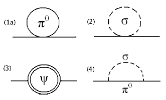
Figure 4: Diagrams that contribute to the $\pi_{0}$ self energy corrections, $\Sigma_{\pi^{0}}(\beta)$

whereas for the charged pions we have only the two diagrams shown in Fig.5.

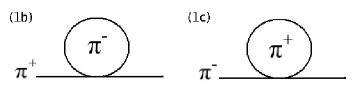
Figure 5: Diagrams that contribute to the $\pi^{+}$, $\pi^{-}$ self energy correction, $\Sigma_{\pi^{+}}(\beta,\mu_{I})$ and $\Sigma_{\pi^{-}}(\beta,\mu_{I})$

The self energy corrections $\sum$ allow, according to the well known procedure of summing geometric series, to define a dressed mass i.e. $m_{d}^{2}=m^{2}+i\sum$.

$\sum$ can be decomposed as $\sum=\sum(0)+\sum(\beta)$, where $\sum(\beta)$ denotes the thermal corrections to the self energy. $\sum(0)$ is the zero temperature self energy and it will not be considered here, since it is absorbed according the usual renormalization procedure at zero temperature.

The self energy correction for $\pi_{0}$ does not depend on the isospin chemical potential $\mu_{I}$, since as we said we are not considering here a $\mu_{I}$ associated to the fermions. On the contrary, the self energy corrections to the charged pions will have now thermal and $\mu_{I}$ dependent contributions.

Our results are plotted in Fig.6 for $\pi_{0}$ and in Fig.7 for the charged pions. The chemical potential contributes, as it was expected to increase de mass for the charged pions.

Figure 6: Mass behavior of $m_{\pi_{0}}$.

Figure 7: Mass behavior of $m_{{\pi}^{+}}$ and $m_{{\pi}^{-}}$.

IV $\sigma$ meson mass corrections

The relevant diagrams, where the $\sigma$ meson is represented by the dashed line, are shown in Fig.8.

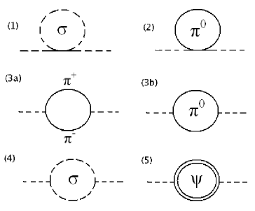
Figure 8: Diagrams that contribute to $\Sigma_{\sigma}(\beta)$

The results for the sigma meson mass are shown in Fig.9 and Fig.10. From the technical point of view, as usual, the principal value has to be use in order to handle the poles.

The growing of $m_{\sigma}$, as function of T, does not correspond to the $m_{\sigma}$ evolution in larsen and in nico . This is due to the Mean Field approximation they followed. In fact, this effective approach is quite more complicated than the usual loop expansion for the masses.

Figure 9: Behavior of $m_{\sigma}$ in function of T.

Figure 10: Behavior of $m_{\sigma}$ in function of $\mu_{I}$.

To summarize, we can see that the isospin chemical potential contribution, both for the masses as well as for the vacuum evolution is quite small compared to the temperature dependence. The pion masses at the one loop order have have a very similar behavior to the corresponding masses in the mean field approaches. However, the sigma meson mass is quite different in both approaches. The loop expansion predicts a steadily growing for the sigma meson mass as function of T with small correction due to $\mu_{I}$.

References

- (1) M.Gell-Mann and M.Lévy, Nuovo Cimento 16,705(1960); see also B.W. Lee, Chiral Dynamics (Gordon and Breach, 1972)
- (2) B.W. Lee, Nucl.Phys. B9 (1969)649; J.L Gervais and Benjamin W. Lee, Nucl. Phys. B12,627(1969).
- (3) J. Gasser and H. Leutwyler, Nucl. Phys. B250, 465 (1985).
- (4) M. Loewe and C. Villavicencio, Phys. Rev. D 67, 074034 (2003); ibid Phys. Rev. D. 70, 074005(2004).
- (5) C.Contreras and M. Loewe, Int. Jour. of Mod. Phys. A5, 2297 (1990).
- (6) A. Larsen, Z.Phys.C 33, 291(1986).
- (7) N.Bilić and H.Nikolić, Eur. Phys. J. C6 513(1999).
- (8) See for example J. B. Kogut and M. A. Stephanov The Phases of Quantum Chromodynamics Cambridge University Press, 2004, and references therein.
- (9) Hong Mao, N. Petopoulos and Wei-Qin Zhao, J.Phys. G32, 2187(2006); N. Petropoulos, arXiv: hep-ph/0402136 and references therein.
- (10) Lianyi He, Meng Jin and Pengfei Zhuang, Phys. Rev. D 71, 116001, 2005.
- (11) H. A. Weldon. Phys. Rev., D26, 1394(1982).
- (12) A. Actor. Phys. Lett., B157, 53(1985).
- (13) E791 Collaboration, E.M. Aitala, etal , Phys. Rev. Lett. 86, 765 (2001), ibid Phys. Rev. Lett. 86, 770 (2001); J.M. de Miranda, I.Bediaga: Scalar meson sigma (500) phase motion at . AID conf. Proc. 814: 654(2006).
- (14) B. W. Lee. Chiral Dynamics. Gordon and Breach 1970.