Braneworld Quintessential Inflation and Sum of Exponentials Potentials

Abstract

Quintessential inflation—in which a single scalar field plays the role of the inflaton and quintessence—from a sum of exponentials potential $V=A\left(e^{5\varphi}+e^{\sqrt{2}\varphi}\right)$ or $V=A\left(e^{5\varphi}+e^{\varphi}\right)$ or a cosh potential $V=2A\cosh(5\varphi)$ is considered in the context of five-dimensional gravitation with standard model particles confined to our 3-brane. Reheating is accomplished via gravitational particle production and the universe undergoes a transition from primordial inflation to radiation domination well before big bang nucleosynthesis. The transition to an accelerating universe due to quintessence occurs near $z\approx 1$, as in $\Lambda$CDM.

Braneworld quintessential inflation can occur for potentials with or without a minimum, and with or without eternal acceleration and an event horizon. The low $z$ behavior of the equation of state parameter $w_{\phi}$ provides a clear observable signal distinguishing quintessence from a cosmological constant.

1 Introduction

In five-dimensional gravitation with standard model particles confined to our 3-brane, the Friedmann equation is modified [1]–[3] at high energies: the square $H^{2}$ of the Hubble parameter acquires a term quadratic in the energy density, allowing [4] slow-roll inflation to occur for potentials that would be too steep to support inflation in the standard Friedmann-Robertson-Walker cosmology. In this model, quintessential inflation—in which a single scalar field plays the role of the inflaton and quintessence—can occur for a sum of exponentials or cosh potential, a type of potential that arises naturally in M/string theory for combinations of moduli fields or combinations of the dilaton and moduli fields.

Inflation ends in this model as the quadratic term in energy density in $H^{2}$ decays to roughly the same order of magnitude as the standard linear term (technically, when the slow-roll parameter $\epsilon$ = 1). Reheating can be accomplished [5] via gravitational particle production at the end of inflation. The universe subsequently [5] undergoes a transition from the era dominated by the scalar field potential energy to an era of “kination” dominated by the scalar field kinetic energy, and then to the standard radiation dominated era well before big-bang nucleosynthesis (BBN). With a sum of exponentials or cosh potential, the universe evolves at this point according to the quintessence/cold dark matter (QCDM) model. The transition to an accelerating universe due to quintessence occurs late in the matter dominated era near $z\approx 1$, as in $\Lambda$CDM.

We will assume a flat universe after inflation. In the QCDM model, the total energy density $\rho=\rho_{m}+\rho_{r}+\rho_{\phi}=\rho_{c}$, where $\rho_{c}$ is the critical energy density for a flat universe and $\rho_{m}$, $\rho_{r}$, and $\rho_{\phi}$ are the energy densities in (nonrelativistic) matter, radiation, and the quintessential inflation scalar field $\phi$, respectively. Ratios of energy densities to the critical energy density will be denoted by $\Omega_{m}=\rho_{m}/\rho_{c}$, $\Omega_{r}=\rho_{r}/\rho_{c}$, and $\Omega_{\phi}=\rho_{\phi}/\rho_{c}$, while ratios of present energy densities $\rho_{m0}$, $\rho_{r0}$, and $\rho_{\phi 0}$ to the present critical energy density $\rho_{c0}$ will be denoted by $\Omega_{m0}$, $\Omega_{r0}$, and $\Omega_{\phi 0}$, respectively.

Using WMAP3 [6] central values, we will set $\Omega_{\phi 0}$ = 0.74, $\Omega_{r0}=8.04\times 10^{-5}$, $\Omega_{m0}=1-\Omega_{\phi 0}-\Omega_{r0}\approx 0.26$, and $\rho_{c0}^{1/4}=2.52\times 10^{-3}$ eV, with the present time $t_{0}=13.7$ Gyr after the big bang.

For the sum of exponentials potential, we will take a monotonically increasing function of $\varphi$ ($\varphi$ will evolve from $\varphi_{i}\gg 1$ at the end of inflation to $|\varphi_{0}|\sim 1$ today)

$$V(\varphi)=A\left(e^{\lambda\varphi}+Be^{\mu\varphi}\right)$$ (1)

where $A$ and $B$ are positive constants, $\lambda>\mu>0$, $\varphi=\phi/M_{P}$, the (reduced) Planck mass $M_{P}=2.44\times 10^{18}$ GeV, and with $\lambda=5$, $\mu=\sqrt{2}$ or 1, and $B=1$ for the simulations. We will also discuss the simple exponential potential $V(\varphi)=Ae^{\lambda\varphi}$ considered in Ref. [5] and the cosh potential $V(\varphi)=2A\cosh(\lambda\varphi)$ with $\lambda=5$. For all four potentials, $V\sim Ae^{\lambda\varphi}$ for $\varphi\gg 1$ (which will be the case during inflation and gravitational particle production). The constant $A\sim\rho_{c0}$ for quintessential inflation (see Table 1).

Note that the BBN ($z\sim 10^{9}$–$10^{11}$), cosmic microwave background (CMB) ($z\sim 10^{3}$–$10^{5}$), and large-scale structure (LSS) ($z\sim 10$–$10^{4}$) bounds $\Omega_{\phi}\stackrel{{\scriptstyle<}}{{\mbox{\scriptsize$\sim$}}}0.1$ are satisfied in all the simulations below (Figs. 3, 8, and 12) and that the transition from the era of scalar field dominance to the radiation era occurs around $z\approx 10^{15}/\lambda$.

Quintessential inflation in the standard cosmology from a sum of exponentials potential was considered in Ref. [7] for $\lambda=20$ and $\mu=0.5$ or $-20$. Ref. [8] extended the analysis to the braneworld case where $H^{2}$ has a quadratic term in energy density, for $\lambda\approx 20$ and $\mu\approx-\lambda$. Braneworld quintessential inflation is also discussed in Ref. [9], for $\lambda=4$ and $\mu=0.1$. Only one simulation for the sum of exponentials potential braneworld scenario is presented, in Ref. [9] for the equation of state parameter $w_{\phi}$. We find that the case $\lambda=4$ and $\mu=0.1$ violates even the looser CMB bound $\Omega_{\phi}\leq 0.2$ (see Fig. 1), and that the recent average of the scalar field equation of state parameter $\overline{w}_{0}=-0.68$ is too large.

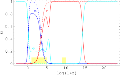
Figure 1: $\Omega$ for $V=A\left(e^{4\varphi}+e^{0.1\varphi}\right)$ (solid) vs. $\Lambda$CDM (dotted). The light yellow rectangles are the bounds $\Omega_{\phi}\leq 0.1$ from LSS, CMB, and BBN.

The current investigation furthermore presents detailed simulations and analyses of the evolution of the scalar field and its equation of state, the fractional energy densities in the scalar field, radiation, and matter, and the acceleration parameter in braneworld quintessential inflation for the sum of exponentials and cosh potentials.

2 Cosmological Equations

The homogeneous scalar field—since it is confined to the brane—still obeys the Klein-Gordon equation

$$\ddot{\phi}+3H\dot{\phi}=-\frac{dV}{d\phi}\equiv-V_{\phi}~{}.$$ (2)

The Hubble parameter $H$ is related to the scale factor $a$ and the energy densities in matter, radiation, and the scalar field through the braneworld modified [4] Friedmann equation

$$H^{2}=\left(\frac{\dot{a}}{a}\right)^{2}=\frac{\rho}{3M_{P}^{2}}\left(1+\frac{\rho}{2\sigma}\right)+\Lambda_{4}+\frac{{\cal E}}{a^{4}}$$ (3)

where the energy density

$$\rho=\rho_{\phi}+\rho_{m}+\rho_{r},~{}~{}\rho_{\phi}=\frac{1}{2}\dot{\phi}^{2}+V(\phi),$$ (4)

$\sigma$ is the four-dimensional brane tension, $\Lambda_{4}$ is the four-dimensional cosmological constant, and ${\cal E}$ is a constant embodying the effects of bulk gravitons on the brane. We will set the four-dimensional cosmological constant to zero. The “dark radiation” term ${{\cal E}/a^{4}}$ can be ignored here since it will rapidly go to zero during inflation. Thus for our purposes the modified Friedmann equation takes the form

$$H^{2}=\frac{\rho}{3M_{P}^{2}}\left(1+\frac{\rho}{2\sigma}\right).$$ (5)

In the low-energy limit $\rho\ll\sigma$, the Friedmann equation reduces to its standard form $H^{2}=\rho/(3M_{P}^{2})$.

The conservation of energy equation for matter, radiation, and the scalar field is

$$\dot{\rho}+3H(\rho+P)=0$$ (6)

where $P$ is the pressure. Except near particle-antiparticle thresholds, $P_{m}$ = 0 and $P_{r}=\rho_{r}/3$. Equation (6) gives the evolution of $\rho_{m}$ and $\rho_{r}$, and the Klein-Gordon equation (2) for the weakly coupled scalar field, with

$$P_{\phi}=\frac{1}{2}\dot{\phi}^{2}-V(\phi).$$ (7)

The acceleration equation

$$\frac{\ddot{a}}{a}=-\frac{1}{6M_{P}^{2}}\left(\rho+3P+\frac{\rho}{\sigma}\left(2\rho+3P\right)\right)$$ (8)

follows from Eqs. (5) and (6). While inflation occurs in the low-energy (standard cosmology) limit when $w\equiv P/\rho<-1/3$, for inflation to occur in the high-energy limit $w<-2/3$.

We will use the logarithmic time variable $\tau=\ln(a/a_{0})=-\ln(1+z)$. Note that for de Sitter space $\tau=H_{\Lambda}t$, where $H_{\Lambda}^{2}=\rho_{\Lambda}/(3M_{P}^{2})$, and that $H_{\Lambda}t$ is a natural time variable for the era of $\Lambda$-matter domination (see e.g. Ref. [10]). For $0\leq z\leq z_{BBN}\sim 10^{10}$, $-23.03\leq\tau\leq 0$, and for $0\leq z\leq z_{Pl}\sim 2.8\times 10^{31}$, $-72.41\leq\tau\leq 0$.

In Eq. (4), we will make the simple approximations

$$\rho_{r}=\rho_{r0}e^{-4\tau},~{}~{}\rho_{m}=\rho_{m0}e^{-3\tau}.$$ (9)

For the spatially homogeneous scalar field $\phi$, the equation of state parameter $w_{\phi}=w_{\phi}(z)=P_{\phi}/\rho_{\phi}$. The recent average of $w_{\phi}$ is defined as

$$\overline{w}_{0}=\frac{1}{\tau}\int_{0}^{\tau}w_{\phi}d\tau.$$ (10)

We will take the upper limit of integration $\tau$ to correspond to $z$ = 1.75. The SNe Ia observations [11] bound the recent average $\overline{w}_{0}<-0.76$ (95% CL) assuming $\overline{w}_{0}\geq-1$, and measure the transition redshift $z_{t}=0.46\pm 0.13$ from deceleration to acceleration (it is probably premature at this point to say more than that $z_{t}\approx 1$).

For numerical simulations, the cosmological equations should be put into a scaled, dimensionless form. Equations (2) and (5) can be cast [12] in the form of a system of two first-order equations in $\tau$ plus a scaled version of $H$:

$$\tilde{H}\varphi^{\prime}=\psi$$ (11)

$$\tilde{H}(\psi^{\prime}+\psi)=-3\tilde{V}_{\varphi}$$ (12)

$$\tilde{H}^{2}=\tilde{\rho}\left(1+\frac{\tilde{\rho}}{2\tilde{\sigma}}\right)$$ (13)

$$\tilde{\rho}=\frac{1}{6}\psi^{2}+\tilde{V}+\tilde{\rho}_{m}+\tilde{\rho}_{r}$$ (14)

where $\psi\equiv e^{2\tau}\dot{\varphi}/H_{0}$, $\tilde{H}=e^{2\tau}H/H_{0}$, $\tilde{V}=e^{4\tau}V/\rho_{c0}$, $\tilde{V}_{\varphi}=e^{4\tau}V_{\varphi}/\rho_{c0}$, $\tilde{\rho}=e^{4\tau}\rho/\rho_{c0}$, $\tilde{\rho}_{m}=e^{4\tau}\rho_{m}/\rho_{c0}=\Omega_{m0}e^{\tau}$, $\tilde{\rho}_{r}=e^{4\tau}\rho_{r}/\rho_{c0}=\Omega_{r0}$, $\tilde{\sigma}=e^{4\tau}\sigma/\rho_{c0}$, and where a prime denotes differentiation with respect to $\tau$: $\varphi^{\prime}=d\varphi/d\tau$, etc.

This scaling results in a set of equations that is numerically more robust, especially before the time of BBN.

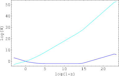
Figure 2: Log₁₀ of $\tilde{H}$ (blue, bottom) and $H/H_{0}$ (cyan, top) vs. $\log_{10}(1+z)$ for $V=A\left(e^{5\varphi}+e^{\sqrt{2}\varphi}\right)$.

Figure 2 illustrates that while $\tilde{H}$ spans only ten orders of magnitude between $z_{i}\sim 10^{23}$ and the present, $H/H_{0}$ spans more than fifty orders of magnitude.

3 Evolution of the Braneworld Universe

In this section, we will closely follow the analyses of Refs. [5] and [4].

3.1 Slow-Roll Braneworld Inflation

The inflationary slow-roll parameter $\epsilon$ is given by [4]

$$\epsilon\equiv-\frac{\dot{H}}{H^{2}}\approx\frac{M_{P}^{2}}{2}\left(\frac{V_{\phi}}{V}\right)^{2}\frac{1+V/\sigma}{(1+V/(2\sigma))^{2}}~{}.$$ (15)

(The slow-roll parameter

$$\eta=M_{P}^{2}\frac{V_{\phi\phi}}{V}\frac{1}{1+V/(2\sigma)}\approx\epsilon$$ (16)

for the potentials considered here.) Inflation occurs for $\epsilon<1$. The slow-roll parameter can be approximated during inflation by

$$\epsilon\approx\frac{2\lambda^{2}\sigma}{V}$$ (17)

for the sum of exponentials potential, the simple exponential potential, and the cosh potential, since $V\gg\sigma$ and $\varphi\gg 1$ for our models during inflation. Inflation ends when $\epsilon=1$, implying [5] that the potential $V_{e}$ at the end of inflation is

$$V_{e}\approx 2\lambda^{2}\sigma.$$ (18)

To evaluate $V_{e}$ and $\sigma$, the COBE-measured amplitude of primordial density perturbations is matched against the theoretical value at $N$ = 50 e-folds from the end of inflation, where

$$N=\int_{t_{N}}^{t_{e}}Hdt\approx\frac{1}{M_{P}^{2}}\int_{\phi_{e}}^{\phi_{N}}\frac{V}{V_{\phi}}\left(1+\frac{V}{2\sigma}\right)d\phi\approx\frac{1}{2\lambda^{2}\sigma}(V_{N}-V_{e})$$ (19)

yielding $V_{N}\approx(N+1)V_{e}$. Now matching against the amplitude [4] of density fluctuations

$$\left(2\times 10^{-5}\right)^{2}=A_{S}^{2}\approx\frac{1}{75\pi^{2}M_{P}^{6}}\frac{V^{3}}{V_{\phi}^{2}}\left(1+\frac{V}{2\sigma}\right)^{3}\approx\frac{1}{600\pi^{2}}\frac{V^{4}}{M_{P}^{4}\lambda^{2}\sigma^{3}}$$ (20)

gives [5]

$$V_{e}^{1/4}\approx 1.11\times 10^{15}~{}{\rm GeV}/\lambda,~{}~{}\sigma^{1/4}\approx 9.37\times 10^{14}~{}{\rm GeV}/\lambda^{3/2}.$$ (21)

3.2 Gravitational Reheating and Initial Conditions

At the end of inflation, gravitational particle production [13]–[15] results in a radiation energy density [5]

$$\frac{\rho_{r}}{\rho_{\phi}}\approx 0.01g_{p}\frac{H_{e}^{4}}{V_{e}}\approx 2.8\times 10^{-4}g_{p}\frac{V_{e}^{3}}{M_{P}^{4}\sigma^{2}}\approx 4.86\times 10^{-17}g_{p}$$ (22)

where $g_{p}\approx$ 10–100 is the number of particle species that are gravitationally produced. This relation fixes the “initial conditions” redshift $z_{i}\approx 3.89\times 10^{23}g_{p}^{1/4}/\lambda$ at which gravitational particle production occurs, from the scaling

$$\rho_{r}\approx 4.86\times 10^{-17}g_{p}\rho_{\phi}\approx g_{p}\left(\frac{10^{11}~{}{\rm GeV}}{\lambda}\right)^{4}\approx(1+z_{i})^{4}\rho_{r0}$$ (23)

corresponding [5] to a reheating temperature

$$T_{e}\sim\left(\frac{g_{p}}{g_{*}}\right)^{1/4}\frac{10^{11}~{}{\rm GeV}}{\lambda}$$ (24)

where $g_{*}(T)$ is the effective number of massless degrees of freedom at temperature $T$. The universe undergoes [5] a transition from the era dominated by the scalar field potential energy to an era of kination ($\rho_{\phi}\sim 1/a^{6}$) dominated by the scalar field kinetic energy as the $\rho^{2}/(2\sigma)$ term in $H^{2}$ becomes small compared with $\rho$. For this era of kination to occur, the potential $V$ must be sufficiently steep. Since during kination $\rho_{r}/\rho_{\phi}\sim a^{2}$, the universe eventually makes a transition [5] to the standard radiation dominated era, around a temperature $T\approx 10^{3}$ GeV$/\lambda$, well before big-bang nucleosynthesis at $T\approx$ 1 MeV. For the sum of exponentials or cosh potential, the universe then evolves according to the QCDM model. The transition to an accelerating universe due to quintessence occurs late in the matter dominated era near $z\approx 1$, as in $\Lambda$CDM.

The initial conditions at the end of inflation will be set in the high-energy, slow-roll limit. The initial value for $\phi_{i}$ is specified by Eq. (18). The initial value for $\dot{\phi}_{i}$ follows from the high-energy, slow-roll limits

$$H^{2}\approx\frac{\rho^{2}}{6M_{P}^{2}\sigma}\approx\frac{V^{2}}{6M_{P}^{2}\sigma}$$ (25)

and

$$\ddot{\phi}+3H\dot{\phi}\approx\sqrt{\frac{3}{2}}\frac{V}{M_{P}\sqrt{\sigma}}\dot{\phi}\approx-V_{\phi}\approx-\lambda\frac{V}{M_{P}}$$ (26)

or [4]

$$\frac{1}{2}\dot{\phi}_{i}^{2}\approx\frac{V_{e}}{6}\approx\frac{1}{3}\lambda^{2}\sigma.$$ (27)

4 Simulations

For the computations below, we will use Eqs. (11)–(14) with initial conditions specified at $z_{i}$ by $\varphi_{i}$ and $\dot{\varphi}_{i}\propto\psi_{i}$ (Eqs. (18) and (27)). We set $\lambda$ = 5 and $g_{p}$ = 100. The constant $A$ in the potentials is adjusted so that $\Omega_{\phi 0}$ = 0.74. This involves the usual single fine tuning. The final time $t_{f}$ is set by $z_{f}=-0.999$ corresponding to $t_{f}\sim$ 100 Gyr.

First we briefly summarize the properties of the exponential potential, and then turn our attention to the quintessential inflation potentials.

$V(\varphi)/A$	$A/\rho_{c0}$	$\varphi_{i}$	$\varphi_{0}$	$\overline{w}_{0}$
$2\cosh(5\varphi)$	0.4	48.0	$-0.03$	$-0.87$
$e^{5\varphi}+e^{\sqrt{2}\varphi}$	5.7	47.4	$-1.60$	$-0.78$
$e^{5\varphi}+e^{\varphi}$	2.2	47.6	$-1.18$	$-0.89$

Table 1: Simulation results for the cosh and sum of exponentials potentials.

4.1 Exponential Potential

The exponential potential $V(\varphi)=Ae^{\lambda\varphi}$ [15]–[18] can be derived from M-theory [19] or from $N$ = 2, 4D gauged supergravity [20].

For the exponential potential with $\lambda^{2}>3$, the cosmological equations have a global attractor with $\Omega_{\phi}=3/\lambda^{2}$ during the matter dominated era (during which $w_{\phi}=0$); and with $\lambda^{2}>4$, the cosmological equations have a global attractor with $\Omega_{\phi}=4/\lambda^{2}$ during the radiation dominated era (during which $w_{\phi}=1/3$). For $\lambda^{2}<3$, the cosmological equations have a late time attractor with $\Omega_{\phi}=1$ and $w_{\phi}=\lambda^{2}/3-1$.

For $\lambda=\sqrt{2}$ and $\rho_{m}=0$, $\ddot{a}\rightarrow 0$ asymptotically; if $\rho_{m}>0$, the universe eventually enters a future epoch of deceleration. In either case, there is no event horizon. For $\lambda<\sqrt{2}$, the universe enters a period of eternal acceleration with an event horizon. For $\lambda>\sqrt{2}$, the universe eventually decelerates and there is no event horizon.

The $\Lambda$CDM cosmology is approached for $\lambda\leq 1/\sqrt{3}$. Significant acceleration occurs only for $\lambda\stackrel{{\scriptstyle<}}{{\mbox{\scriptsize$\sim$}}}\sqrt{3}$. For $\lambda=\sqrt{3}$, $\overline{w}_{0}$ is much too high; for a viable present-day QCDM cosmology, $\lambda\leq\sqrt{2}$ [12] in the exponential potential.

4.2 Cosh Potential

In the cosh potential model

$$V=2A\cosh(5\varphi)\approx\rho_{\Lambda}\cosh(5\varphi),$$ (28)

dark energy derives from the value of the potential near its minimum. This is the simplest way to “correct” the exponential potential to incorporate quintessence.

In the simulations for the cosh potential (Figs. 3–7), initially $\varphi\approx 50$ and then evolves to $\varphi_{0}=-0.03$ at $t_{0}$. The linear decay of $\varphi(\tau)$ in Fig. 4 during the kination era occurs because $\rho_{\phi}\approx\frac{1}{2}\dot{\phi}^{2}\sim 1/a^{6}$ and thus $\varphi^{\prime}$ is a (negative) constant since both $\tilde{H}$ and $\psi$ are proportional to $e^{-\tau}$ in Eq. (11).

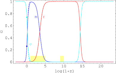
Figure 3: $\Omega$ for $V=2A\cosh(5\varphi)$ (solid) vs. $\Lambda$CDM (dotted).

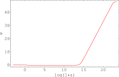
Figure 4: $\varphi$ for $V=2A\cosh(5\varphi)$.

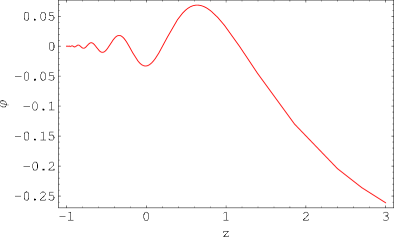
Figure 5: Oscillating behavior of $\varphi$ near $z=0$ for $V=2A\cosh(5\varphi)$.

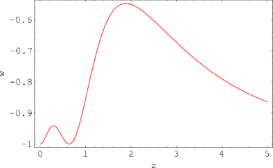
Figure 6: $w_{\phi}$ for $V=2A\cosh(5\varphi)$.

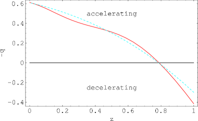
Figure 7: Acceleration parameter $-q$ for $V=2A\cosh(5\varphi)$ (solid) vs. $\Lambda$CDM (dotted).

Between $z\approx 2.5\times 10^{14}$ (as the universe enters its radiation dominated stage) and $z\approx 10$ (when $m_{\phi}^{2}\approx\lambda^{2}V/M_{P}^{2}$ becomes of order $H^{2}\approx\rho_{m}/(3M_{P}^{2})$), $\varphi$ “sits and waits” at a small negative value.

With the cosh potential, $\varphi$ is very slowly oscillating and decaying about $\varphi=0$ at the minimum of the potential for $z\stackrel{{\scriptstyle<}}{{\mbox{\scriptsize$\sim$}}}1$ (we have neglected any present-day particle production by the oscillating scalar field), with angular frequency $\omega\approx\sqrt{3}\lambda H_{\Lambda}$ and decay time constant $\overline{t}\approx 2H_{\Lambda}^{-1}/3$ (see Fig. 5).

Note that $w_{\phi}\rightarrow-1$ for $t>t_{0}$ (Fig. 6). The acceleration parameter $-q$ in Fig. 7 closely mimics the $\Lambda$CDM curve.

4.3 Sum of Exponentials Potential

In the sum of exponentials potential (1), a shift $\varphi\rightarrow\varphi+\chi$ simply results in a redefinition of the constants $A$ and $B$:

$$V(\varphi)\rightarrow V(\varphi+\chi)={\cal A}\left(e^{\lambda\varphi}+{\cal B}e^{\mu\varphi}\right),~{}~{}{\cal A}=e^{\lambda\chi}A,~{}~{}{\cal B}=e^{(\mu-\lambda)\chi}B.$$ (29)

In a realistic particle theory $A$ and $B$ would be set from first principles; here we choose $B=1$. It will turn out then that $A\sim\rho_{c0}$ for quintessential inflation.

To produce primordial inflation in the braneworld scenario with the sum of exponentials potential and the subsequent transition to the standard radiation dominated universe satisfying the constraints on $\Omega_{\phi}$, $\lambda\stackrel{{\scriptstyle>}}{{\mbox{\scriptsize$\sim$}}}4.7$ (this agrees with the estimate $\lambda\stackrel{{\scriptstyle>}}{{\mbox{\scriptsize$\sim$}}}4.5$ given in Ref. [5]); for present-day quintessence, $\mu\leq\sqrt{2}$ [12]. We will choose $\lambda=5$ and $\mu=\sqrt{2}$ or 1 (these values appear naturally in low-energy limits of M/string theory):

$$V(\varphi)=A\left(e^{5\varphi}+e^{\sqrt{2}\varphi}\right)$$ (30)

or

$$V(\varphi)=A\left(e^{5\varphi}+e^{\varphi}\right).$$ (31)

For the sum of exponentials potentials (Figs. 8–15), initially $\varphi\approx 50$ and then evolves to $\varphi_{0}\sim-1$. Again note the the linear decay of $\varphi(\tau)$ in Figs. 9 and 13 during the kination era.

Figure 8: $\Omega$ for $V=A\left(e^{5\varphi}+e^{\sqrt{2}\varphi}\right)$ (solid) vs. $\Lambda$CDM (dotted).

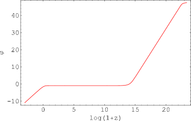
Figure 9: $\varphi$ for $V=A\left(e^{5\varphi}+e^{\sqrt{2}\varphi}\right)$.

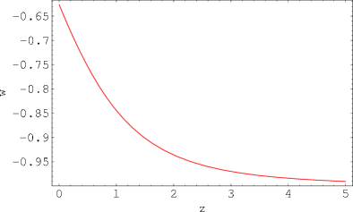
Figure 10: $w_{\phi}$ for $V=A\left(e^{5\varphi}+e^{\sqrt{2}\varphi}\right)$.

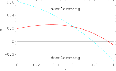
Figure 11: Acceleration parameter $-q$ for $V=A\left(e^{5\varphi}+e^{\sqrt{2}\varphi}\right)$ (solid) vs. $\Lambda$CDM (dotted).

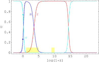
Figure 12: $\Omega$ for $V=A\left(e^{5\varphi}+e^{\varphi}\right)$ (solid) vs. $\Lambda$CDM (dotted).

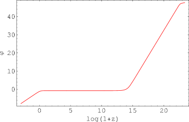
Figure 13: $\varphi$ for $V=A\left(e^{5\varphi}+e^{\varphi}\right)$.

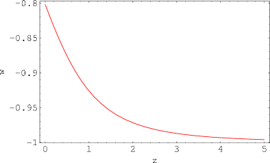
Figure 14: $w_{\phi}$ for $V=A\left(e^{5\varphi}+e^{\varphi}\right)$.

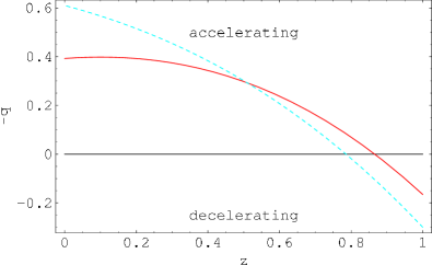
Figure 15: Acceleration parameter $-q$ for $V=A\left(e^{5\varphi}+e^{\varphi}\right)$ (solid) vs. $\Lambda$CDM (dotted).

Between $z\approx 2.5\times 10^{14}$ and $z\approx 2$ (when now $m_{\phi}^{2}\approx\mu^{2}V/M_{P}^{2}$ becomes of order $H^{2}\approx\rho_{m}/(3M_{P}^{2})$), $\varphi$ “sits and waits” at a small negative value, and then becomes more negative. The linear decay of $\varphi(\tau)$ after $t_{0}$ occurs because $\varphi$ is approaching the late time attractor with $\Omega_{\phi}=1$ and $w=\mu^{2}/3-1$ (Figs. 10 and 14). Whenever $w$ = const and $H$ approximates its standard form, $\varphi(\tau)$ is linear in $\tau$ since both $\tilde{H}$ and $\psi$ are proportional to $e^{(1-3w)\tau/2}$ in Eq. (11) ($w=1$ during kination).

Note the differences in the acceleration parameter $-q$ in Figs. 11 and 15 for the two cases $\mu=\sqrt{2}$ (eventual deceleration with no event horizon) and $\mu=1$ (eternal acceleration with an event horizon).

5 Conclusion

In the braneworld framework, the sum of exponentials and cosh potentials yield natural quintessential inflation scenarios, motivated by string/M theory. The quintessential braneworld models also provide—through an era of kination—a natural mechanism for the transition of the universe from the primordial $\phi$-dominated era to the era of radiation domination.

From the time of radiation domination to the distant future, $\Omega_{\phi}$ mimics $\Omega_{\Lambda}$ for the quintessential inflation potentials presented here. In the $\Lambda$CDM model and in braneworld quintessential inflation from a cosh or sum of exponentials potential, there is a period between roughly 3.5 Gyr and 20 Gyr after the big bang when $0.1\leq\Omega_{\phi}\leq 0.9$.

Note that for the cosh and sum of exponentials potentials $\overline{w}_{0}\leq-0.78$ (see Table 1), satisfying the observational bound $\overline{w}_{0}<-0.76$.

Braneworld quintessential inflation can occur for potentials with (cosh) or without (sum of exponentials) a minimum, and with (sum of exponentials with $\mu=1$ or cosh) or without (sum of exponentials with $\mu=\sqrt{2}$) eternal acceleration and an event horizon.

In both the cosh and sum of exponentials potentials considered here, the low $z$ behavior of $w_{\phi}$ provides a clear observable signal distinguishing quintessence from a cosmological constant.

References

- [1] P. Binetruy, C. Deffayet, and D. Langlois, Nucl. Phys. B 565, 269 (2000) [arXiv:hep-th/9905012].
- [2] P. Binetruy, C. Deffayet, U. Ellwanger, and D. Langlois, Phys. Lett. B 477, 285 (2000) [arXiv:hep-th/9910219].
- [3] T. Shiromizu, K. i. Maeda, and M. Sasaki, Phys. Rev. D 62, 024012 (2000) [arXiv:gr-qc/9910076].
- [4] R. Maartens, D. Wands, B. A. Bassett, and I. Heard, Phys. Rev. D 62, 041301 (2000) [arXiv:hep-ph/9912464].
- [5] E. J. Copeland, A. R. Liddle, and J. E. Lidsey, Phys. Rev. D 64, 023509 (2001) [arXiv:astro-ph/0006421].
- [6] D. N. Spergel et al., arXiv:astro-ph/0603449.
- [7] T. Barreiro, E. J. Copeland, and N. J. Nunes, Phys. Rev. D 61, 127301 (2000) [arXiv:astro-ph/9910214].
- [8] A. S. Majumdar, Phys. Rev. D 64, 083503 (2001) [arXiv:astro-ph/0105518].
- [9] N. J. Nunes and E. J. Copeland, Phys. Rev. D 66, 043524 (2002) [arXiv:astro-ph/0204115].
- [10] C. L. Gardner, Phys. Rev. D 68, 043513 (2003) [arXiv:astro-ph/0305080].
- [11] A. G. Riess et al. [Supernova Search Team Collaboration], Astrophys. J. 607, 665 (2004) [arXiv:astro-ph/0402512].
- [12] C. L. Gardner, Nucl. Phys. B 707, 278 (2005) [arXiv:astro-ph/0407604].
- [13] L. H. Ford, Phys. Rev. D 35, 2955 (1987).
- [14] B. Spokoiny, Phys. Lett. B 315, 40 (1993) [arXiv:gr-qc/9306008].
- [15] P. G. Ferreira and M. Joyce, Phys. Rev. D 58, 023503 (1998) [arXiv:astro-ph/9711102].
- [16] C. Wetterich, Nucl. Phys. B 302, 668 (1988).
- [17] E. J. Copeland, A. R. Liddle, and D. Wands, Phys. Rev. D 57, 4686 (1998) [arXiv:gr-qc/9711068].
- [18] M. Doran and C. Wetterich, Nucl. Phys. Proc. Suppl. 124, 57 (2003) [arXiv:astro-ph/0205267].
- [19] P. K. Townsend, JHEP 0111, 042 (2001) [arXiv:hep-th/0110072].
- [20] L. Andrianopoli, M. Bertolini, A. Ceresole, R. D’Auria, S. Ferrara, P. Fré, and T. Magri, J. Geom. Phys. 23, 111 (1997) [arXiv:hep-th/9605032].