MCTP-07-02 Narrow Trans-TeV Higgs Bosons and $H\rightarrow hh$ Decays:
Two LHC Search Paths for a Hidden Sector Higgs Boson

Abstract

We consider the addition of a condensing singlet scalar field to the Standard Model. Such a scenario may be motivated by any number of theoretical ideas, including the common result in string-inspired model building of singlet scalar fields charged under some hidden sector gauge symmetry. For concreteness, we specify an example model of this type, and consider the relevant constraints on Higgs physics, such as triviality, perturbative unitarity and precision electroweak analysis. We then show that there are two unique features of the phenomenology that present opportunities for discovery at the Large Hadron Collider (LHC). First, it is possible to identify and discover a narrow trans-TeV Higgs boson in this scenario — a mass scale that is well above the scale at which it is meaningful to discuss a SM Higgs boson. Second, the decays of the heavier scalar state into the lighter Higgs bosons can proceed at a high rate and may be the first discovery mode in the Higgs sector.

1 Introduction

Nature may contain many more particles than are implied by what we consider at first thought to be well-motivated ideas of new physics. This is especially true if our mindset is entirely on trying to understand electroweak symmetry breaking in the most minimal framework that we can devise. There are many things to explain in nature beyond the Standard Model (SM), and electroweak symmetry breaking (EWSB) is merely one of them.

In the search for beyond Standard Model (SM) physics, hidden sector SM singlet fields are ubiquitous in many existing theories, such as in string-inspired particle physics models containing many more gauge groups and corresponding scalar sectors than would otherwise be needed to describe or contain the SM. Even without these more practical motivations, it is always reasonable to imagine such a ‘phantom’ world and how it can influence the physics of our SM world, since no present experimental data rules out its existence, and we know so little definitively about the Higgs sector.

It would be interesting to pursue whether we can find evidence for the hidden sector at the LHC. In many scenarios, hidden sector fields couple to the SM fields only through non-renormalizable terms or loop effects. In these cases, the discovery of these fields seems not very promising and they may end up to be truly ‘hidden’ at colliders. Fortunately, there are two renormalizable interactions between the hidden sector and the SM fields. The first one is the mixing between $U(1)_{Y}$ and the $U(1)_{hid}$ through the kinetic term $\chi B_{\mu\nu}C^{\mu\nu}$ where $B,C$ are the field strengths of the two Abelian fields, respectively. This consideration leads to $Z^{\prime}$ physics, which has been well studied[1]. In this paper we will focus on the phenomenology of the other possibility which applies to more general hidden gauge structure (not just Abelian groups): the renormalizable interaction of the SM Higgs with the hidden sector Higgs. There are few ways that the SM fields can interact with the hidden sector or phantom sector fields, and the Higgs boson, which can form a gauge-invariant dimension-2 operator all on its own, is a prime candidate to pursue this connection [2, 3, 4, 5, 6].

Concretely, the analysis in this paper is based on the model presented in [2], where the SM Higgs $\Phi_{SM}$ couples to a hidden scalar $\Phi_{H}$ through the renormalizable term $|\Phi_{SM}|^{2}|\Phi_{H}|^{2}$. We also assume that the hidden sector has a rich gauge theory structure which is at least partly broken by $\langle\Phi_{H}\rangle\neq 0$. A nontrivial vev of $\Phi_{H}$ is necessary for the mass mixing between the SM Higgs and $\Phi_{H}$, which results in two mass eigenstates, $h$, $H$. It is this mixing that brings in the two possible distinct signatures at the LHC which are of primary interest in this paper: a narrow width trans-TeV Higgs boson and the observable $H\rightarrow hh$ decay.

Here is the outline of what follows. In section 2, we give a brief review of the model we will analyze. In section 3, we study the bounds on Higgs masses for this model, based on the considerations of perturbative unitarity, triviality and precision electroweak measurements. We find that the canonical constraints on the upper limit of the Higgs mass do not apply for the heavier Higgs boson $H$ because of the mixing effect. Based on the results of the earlier sections, we propose two possible intriguing features to be probed at future colliders: narrow trans-TeV Higgs boson and $H\rightarrow hh$ decay width. In section 4, we study the LHC implications of those two signatures in detail and demonstrate that they can be distinguishable and therefore shed new light on beyond SM physics.

2 Model Review

To be self-contained, we first briefly review the model in [2], which sets the framework and notation for what we analyze here. We assume that there is a hidden $U(1)$ gauge symmetry which is broken by a vacuum expectation value (vev) of the Higgs boson $\Phi_{H}$. We denote the $U(1)_{hid}$ gauge boson as $V$, which gets a mass $m_{V}$ after the breaking of $U(1)_{hid}$. In this model, the hidden sector Higgs boson $\Phi_{H}$ mixes with the SM Higgs $\Phi_{SM}$ through a renormalizable interaction $|\Phi_{SM}|^{2}|\Phi_{H}|^{2}$. The Higgs boson Lagrangian under consideration is

$$\mathcal{L}_{Higgs}=|\mathcal{D}_{\mu}\Phi_{SM}|^{2}+|\mathcal{D}_{\mu}\Phi_{H}|^{2}+m^{2}_{\Phi_{SM}}|\Phi_{SM}|^{2}+m^{2}_{\Phi_{H}}|\Phi_{H}|^{2}-\lambda|\Phi_{SM}|^{4}-\rho|\Phi_{H}|^{4}-\eta|\Phi_{SM}|^{2}|\Phi_{H}|^{2}$$ (1)

The component fields are written as

$$\Phi_{SM}=\frac{1}{\sqrt{2}}\left(\begin{array}[]{c}\phi_{SM}+v+iG^{0}\\ G^{\pm}\\ \end{array}\right),~{}~{}~{}\Phi_{H}=\frac{1}{\sqrt{2}}(\phi_{H}+\xi+iG^{\prime})$$ (2)

where $v$($\simeq 246\,{\rm GeV}$) and $\xi$ are vevs around which the $\Phi_{SM}$ and $\Phi_{H}$ are expanded. The $G$ fields are Goldstone bosons, which can be removed from actual calculation by imposing the unitary gauge. After diagonalizing the mass matrix, we rotate from the gauge eigenstates ${\phi_{SM},\phi_{H}}$ to mass eigenstates ${h,H}$.

$$\phi_{SM} = \cos\omega h+\sin\omega H$$ (3)

$$\phi_{H} = -\sin\omega h+\cos\omega H$$ (4)

the mixing angle $\omega$ and the mass eigenvalues are given by

$$\tan\omega = \frac{\eta v\xi}{(-\lambda v^{2}+\rho\xi^{2})+\sqrt{(\lambda v^{2}-\rho\xi^{2})^{2}+\eta^{2}v^{2}\xi^{2}}}$$ (5)

$$m^{2}_{h,H} = (\lambda v^{2}+\rho\xi^{2})\pm\sqrt{(\lambda v^{2}-\rho\xi^{2})^{2}+\eta^{2}v^{2}\xi^{2}}$$

For simplicity in writing subsequent formula, we assume that $m_{h}<m_{H}$ and write $c_{\omega}\equiv\cos_{\omega}$, $s_{\omega}\equiv\sin_{\omega}$.

If $m_{H}>2m_{h}$, the signature of interest, $H\rightarrow hh$ decay, is allowed kinematically. The partial width of this decay is

$$\Gamma(H\rightarrow hh)=\frac{|\mu|^{2}}{8\pi m_{H}}\sqrt{1-\frac{4m_{h}^{2}}{m_{H}^{2}}}$$ (6)

where $\mu$ is the coupling of the relevant mixing operator in the Lagrangian $\triangle\mathcal{L}_{mix}=\mu h^{2}H$.

$$\mu=-\frac{\eta}{2}(\xi c_{\omega}^{3}+vs_{\omega}^{3})+(\eta-3\lambda)vc_{\omega}^{2}s_{\omega}+(\eta-3\rho)\xi c_{\omega}s_{\omega}^{2}$$ (7)

Before going to the discussion of the Higgs mass bounds, it is helpful to do a parameter space analysis for this model. There are a total of 7 input parameters relevant for most of our later discussion: $g,\lambda,v,\eta,\rho,\xi,g_{V}$, where $g$ is the $SU(2)_{L}$ gauge coupling, $g_{V}$ is defined to be the gauge coupling constant of $U(1)_{hid}$. $g_{V}$ in general would appear in the scattering amplitude of the graphs involving the $U(1)_{hid}$ gauge boson $V$, and therefore play a role in the discussion of perturbative unitarity (however, in section 3.1, we will make a reasonable assumption that results in $g_{V}$ effectively disappearing in all the relevant formulae). Other possible input parameters that describe the details of the matter content of the hidden sector itself are uncertain and we do not include them here (in our work, they are only relevant to the RGE of $\rho$, where we just introduce two representative parameters $E$ and $E^{\prime}$). $g,v$ are already fixed by collider experiments, with the values $v=246$GeV, $g=0.65$. In order to study the phenomenology of the model, we construct some output parameters from these input parameters which are of more physical interest: $m_{W},G_{F},m_{h},s_{\omega},m_{V},G_{F}^{{}^{\prime}},m_{H},\mu$, where we define $G_{F}^{{}^{\prime}}$ as the Fermi coupling for the $U(1)_{hid}$ defined in the same way as $G_{F}$ in the SM. We will see in section 3.1 that $G_{F}^{{}^{\prime}}$ plays an important role in the unitarity bounds. The relevant transformations in addition to eqs. (5)-(7) are:

$$m_{W}=\frac{1}{2}gv,~{}~{}m_{V}=\frac{1}{2}g_{V}\xi,~{}~{}G_{F}=\frac{1}{\sqrt{2}v^{2}},~{}~{}G_{F}^{{}^{\prime}}=\frac{1}{\sqrt{2}\xi^{2}}.$$ (8)

Now we have determined that the 4 most important unknown input parameters are $\{\lambda,\rho,\eta,\xi\}$. The inverse transformation from $\{m_{h}^{2},m_{H}^{2},s_{\omega},\mu\}$ to $\{\lambda,\rho,\eta,\xi\}$ are

$$\lambda = \frac{M^{2}_{11}}{2v^{2}}$$ (9)

$$\rho = \frac{M^{2}_{22}}{2v^{2}s_{\omega}^{2}}\left[\frac{c_{\omega}^{3}M^{2}_{12}+3c_{\omega}^{2}s_{\omega}M_{11}^{2}-2c_{\omega}s_{\omega}^{2}M_{12}^{2}+2\mu v}{-2c_{\omega}^{2}M_{12}^{2}+3c_{\omega}s_{\omega}M_{22}^{2}+s_{\omega}^{2}M^{2}_{12}}\right]^{2}$$ (10)

$$\eta = -\frac{M_{12}^{2}}{s_{\omega}v^{2}}\left[\frac{c_{\omega}^{3}M^{2}_{12}+3c_{\omega}^{2}s_{\omega}M_{11}^{2}-2c_{\omega}s_{\omega}^{2}M_{12}^{2}+2\mu v}{-2c_{\omega}^{2}M_{12}^{2}+3c_{\omega}s_{\omega}M_{22}^{2}+s_{\omega}^{2}M^{2}_{12}}\right]$$ (11)

$$\xi = s_{\omega}v\left[\frac{-2c_{\omega}^{2}M_{12}^{2}+3c_{\omega}s_{\omega}M^{2}_{22}+s_{\omega}^{2}M^{2}_{12}}{-cw^{3}M_{12}^{2}-3c_{\omega}^{2}s_{\omega}M^{2}_{11}+2c_{\omega}s_{\omega}^{2}M^{2}_{12}-2\mu v}\right]$$ (12)

where

$$M^{2}_{11} = c_{\omega}^{2}m_{h}^{2}+s_{\omega}^{2}m_{H}^{2}$$ (13)

$$M^{2}_{12} = c_{\omega}s_{\omega}(m^{2}_{H}-m^{2}_{h})$$ (14)

$$M^{2}_{22} = s_{\omega}^{2}m^{2}_{h}+c_{\omega}^{2}m^{2}_{H}$$ (15)

In Tables 1 and 2 we provide 6 benchmark points in parameter space, some of which will be used in section 4 for collider physics analysis. They all can satisfy the theoretical bounds as we shall see in section 3. We list them in Table 1 and Table 2.

	Point A	Point B	Point C
$s_{\omega}^{2}$	0.40	0.31	0.1
$m_{h}$ (GeV)	143	115	120
$m_{H}$ (GeV)	1100	1140	1100
$\Gamma(H\rightarrow hh)$ (GeV)	14.6	4.9	10
$BR(H\rightarrow hh)$	0.036	0.015	0.095

Table 1: Points illustrating parameters of trans-TeV mass Higgs boson. Point C is studied in detail in section 4.

	Point 1	Point 2	Point 3
$s_{\omega}^{2}$	0.5	0.5	0.5
$m_{h}$ (GeV)	115	175	225
$m_{H}$ (GeV)	300	500	500
$\Gamma(H\rightarrow hh)$ (GeV)	2.1	17	17
$BR(H\rightarrow hh)$	0.33	0.33	0.33

Table 2: Points illustrating parameters that allow large branching fractions of $H\to hh$. Each of these points are studied in detail in section 4.

$\Gamma(H\rightarrow hh)$ for points 1, 2, 3 are obtained based on the assumption that the branching ratio BR$(H\rightarrow hh)=1/3$ where BR$=\frac{\Gamma(H\rightarrow hh)}{\Gamma(H\rightarrow hh)+s_{\omega}^{2}\Gamma^{SM}(m_{H})}$. $\Gamma^{SM}(m_{H})$ is the well-known SM result, which can be obtained from the HDECAY program [7].

3 Theoretical Bounds on Higgs Masses of the Model

3.1 Perturbative Unitarity Constraints

The possibility of a strongly interacting WW sector or Higgs sector above the TeV scale is an interesting alternative to a perturbative, light Higgs boson. However, this possibility implies the unreliability of perturbation theory. Although this is not a fundamental concern, it would imply a challenge to the successful perturbative description of precision electroweak data and would have major implications to LHC results. In order for the perturbative description of all electroweak interactions to be valid up to a high scale, the perturbative unitarity constraint would need to be satisfied. This issue has been carefully studied for the SM Higgs sector[8]. They obtained an upper bound on the Higgs mass by imposing the partial-wave unitarity condition on the tree-level amplitudes of all the relevant scattering processes in the limit $s\rightarrow\infty$, where $s$ is the center of mass energy. The result is $m^{2}_{\phi_{SM}}\leq\frac{4\pi\sqrt{2}}{3G_{F}}\simeq$ (700 GeV)². To get this result, we apply a more restrictive condition as in [9]: $|Rea_{J}|\leq\frac{1}{2}$, where $a_{J}$ is the $J^{\rm th}$ partial wave amplitude. This is also the condition we will apply for our model.

We derive the unitarity constraints for our model by methods analogous to ref. [8]. The addition of one more Higgs and the mixing effects introduce more relevant processes and more complex expressions. We impose the unitarity constraints on both the SM sector and the $U(1)_{hid}$ sector. The analysis for the diagrams involving $V$ is very similar to those involving the $Z$ boson. For simplicity, we assume that in the hidden sector, $m_{V}\ll m_{H}$, as an analogy to the case in the SM, where $m_{W}\ll m_{H}$. With this approximation, $g_{V}$ will not appear in the scattering amplitude, only $G_{F}^{\prime}$ is relevant. We list the set of 15 inequalities in the Appendix, and their corresponding processes. For simplicity, we did not transform them to purely input or output parameter basis, but kept them in a mixing form as they were derived for compact expressions. Unlike the situation in SM, it would be hard to solve this complex set of inequalities analytically to get the Higgs mass bounds. Instead using the Monte Carlo method, we generated $60^{4}\sim 10^{7}$ points in the input parameter space with basis $\{\lambda,\eta,\rho,\xi\}$. In order to be consistent with our discussion of perturbative TeV physics, we liberally set the allowed regions of these input parameters to be:

$$\lambda\subset[0,4\pi],\rho\subset[0,4\pi],\eta\subset[-4\pi,4\pi],\xi\subset[0,5\,{\rm TeV}]$$ (16)

Then we pick out the points that satisfy all 15 inequalities, and make $m_{H}-m_{h}$ plots for certain narrow ranges of the mixing angle $s_{\omega}^{2}$ which is an important output parameter for collider physics study. The allowed region can be read from the shape of these plots (obviously, for this multi-dimension parameter space, the bounds on Higgs mass are dependent on the mixing angle).

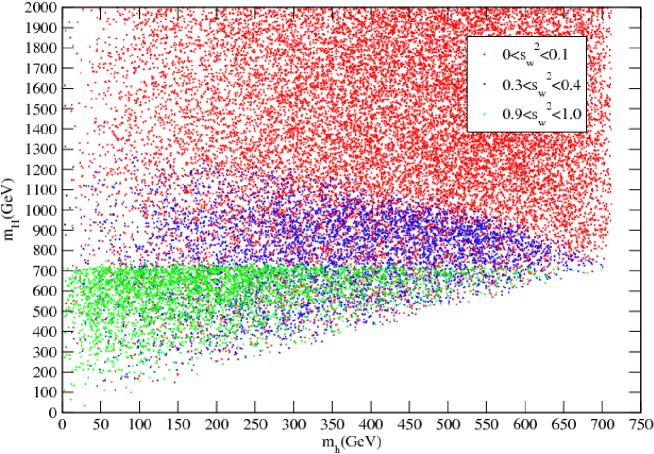
Figure 1: Scatter plot of solutions in the $m_{H}$ vs. $m_{h}$ plane that satisfies perturbative unitarity constraints. Separate colors are used depending on what range $s^{2}_{\omega}$ falls within.

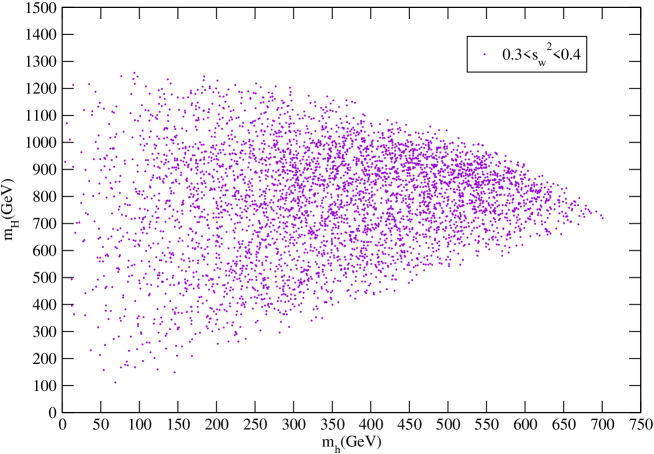
Figure 2: Scatter plot of solutions in the $m_{H}$ vs. $m_{h}$ plane that satisfies perturbative unitarity constraints. This plot is only for points that fall within $0.3<s^{2}_{\omega}<0.4$.

Fig. 1 combines the plots for 3 typical mixing regions – small mixing, medium mixing and large mixing for comparison. We can tell that for the lighter physical Higgs boson mass, the upper bound always stays the same as the well-known SM case—around 700 GeV. However, for the heavier Higgs boson in the spectrum, the bound is loosened: for small mixing it can be as high as 15 TeV given our parameter ranges (in Fig. 1, we cut the upper limit at 2 TeV to reduce the size of the graph as well as improve the presentability of the graph), for medium mixing can be above 1 TeV — both are well above the canonical upper limit of the Higgs boson mass based on unitarity considerations. For large mixing limit, the canonical 700 GeV bound applies for both of the physical Higgs. These observations agree with our intuition. The intermediate mixing region is of significant phenomenological interest, since it can not only generate a heavy Higgs boson — especially a trans-TeV Higgs which is not well anticipated by the experiments, yet may be worth attention — but also can produce the heavy Higgs boson at a considerable production rate at colliders (we know that the coupling of $H$ to SM particles is proportional to $s_{\omega}$). That is why we amplify the plot for the medium mixing region in Fig. 2 to demonstrate the bound shape more clearly. Meanwhile, the small mixing region can also be interesting, since as $s_{\omega}$ decreases, the decay width narrows down which is good for detection, although the production rate gets lower.

Based on the considerations described above, we choose 3 typical points from those that are allowed by all the perturbative unitarity bounds and can generate a trans-TeV Higgs: points A, B and C, as we listed in Table 1 at the end of section 2. They are labelled by the output parameter basis $\{s_{\omega}^{2},m_{h},m_{H},\Gamma(H\rightarrow hh)\}$. Point A and B are from medium mixing region ($s_{\omega}^{2}=0.40$ for point A is actually the maximum mixing angle that can allow a $m_{H}$ larger than 1.1 TeV among all the points that satisfy unitarity constraints), point C is from the small mixing region. We will make precision electroweak analysis for these 3 points in section 3.3 and study the collider physics of trans-TeV Higgs bosons in section 4.1.

3.2 Triviality bounds and Vacuum Stability Bounds

Besides perturbative unitarity, triviality and vacuum stability are two additional concerns which impose theoretical constraints on the Higgs mass. Now we want to see if they would put more stringent bounds on the Higgs mass than those given by unitarity. In the SM, both of them are actually relevant to the properties of the parameter $\lambda$ at the high scale, which are analyzed using the RG equation of $\lambda$. The triviality bound is given based on the requirement that the Landau pole of $\lambda$ from the low-scale theory perspective is above the scale of new physics. The vacuum stability bound is given based on the requirement that $\lambda$ remains positive up to the scale of new physics. Now we already can see that the bounds derived from these two considerations are not definite, as they depend on the scale of new physics. In the SM, the bounds for the value of $\lambda$ at the electroweak scale are equivalent to the upper and lower limits for Higgs boson because of the simple proportion relation $m_{\Phi_{SM}}^{2}=2\lambda v^{2}$, where $v\simeq 246\,{\rm GeV}$. As reviewed in [10], for a $1\,{\rm TeV}$ new physics scale, $160\,{\rm GeV}<m_{H}<750\,{\rm GeV}$. (This is actually a rough estimation based on 1-loop RGE and without taking into threshold corrections. More accurate analysis would be subtle.) However, it is easy to tell that these constraints do not apply for our model where the physical Higgs spectra are determined by four input parameters $\lambda,\eta,\rho,\xi$, not just $\lambda$. Therefore, we need to first derive the RG equations for all these four parameters and see what we can say for the Higgs mass bounds based on them.

Here we give the 1-loop results. For convenience, we suppose that the RGEs run above the EWSB scale, so that all the masses are zero and we can safely work with gauge eigenstates. (Actually, as is well known, the RGEs of dimensionless couplings are independent of mass parameters, which supports the validity of our assumption.)

1-loop RGE for $\lambda$ in the SM can be found in [9]. The addition of the hidden sector Higgs boson contributes another term to the RGE, which results from the mixing term in the Lagrangian $\frac{1}{4}\eta\phi_{H}^{2}\phi_{SM}^{2}$ ($\phi_{H}$ runs in the loop). The full result is:

$$\frac{d}{dt}\lambda=\frac{1}{16\pi^{2}}\left\{\frac{1}{2}\eta^{2}+12\lambda^{2}+6\lambda y_{t}^{2}-3y_{t}^{4}-\frac{3}{2}\lambda(3g^{2}+g^{2}_{1})+\frac{3}{16}[2g^{4}+(g^{2}+g_{1}^{2})^{2}]\right\}$$ (17)

where $g_{1}$ is the gauge coupling of $U(1)_{Y}$, $y_{t}$ is the top Yukawa coupling. The first term comes from the interaction between $\phi_{H}$ and $\phi_{SM}$.

For $\rho$, there is also a 1-loop contribution from the graph where $\phi_{SM}$ runs in the loop. The other terms in the RGE of $\rho$ come from the self-interactions in the hidden sector, e.g. the coupling between $\phi_{H}$ and the hidden sector matter—we denote all these terms by $E$. The result is

$$\frac{d}{dt}\rho=\frac{1}{16\pi^{2}}(\eta^{2}+10\rho^{2}+E)$$ (18)

The RGE of $\eta$ involves only two graphs: with $\phi_{SM}$ or $\phi_{H}$ running in the loop. We eventually get:

$$\frac{d}{dt}\eta=\frac{1}{16\pi^{2}}\eta\left[6\lambda+4\rho+2\eta+3y_{t}^{2}-\frac{3}{4}(3g^{2}+g^{2}_{1})+E^{\prime}\right]$$ (19)

We can see from eqs.(17)-(19) that the perturbative properties of $\lambda$, $\rho$ and $\eta$ can be nice although they are model dependent. However, we can hardly draw any quantitative conclusions regarding, especially, the Higgs masses bounds – they depend on four unknown parameters, the detailed content of hidden sector matter represented by parameters $E$ and $E^{\prime}$, threshold corrections, etc. All of these uncertainties make the prediction for the triviality and stability bounds quite model dependent. Meanwhile, such large freedom allows us to reasonably expect that the points that satisfy the unitarity conditions are also allowed by triviality and stability constraints in a large region of full parameter space (with parameters for hidden sector itself included). A practical application of this observation is that now we can reasonably assume that the points from section 3.1 can also pass the test of triviality and vacuum stability.

3.3 Contraints from Precision Electroweak Measurements

Precision electroweak measurements also give indirect bounds on the Higgs boson mass based on the fact that the virtual excitations of the Higgs boson can contribute to physical observables, e.g. W boson mass, considered in precision tests of the SM. For the one doublet Higgs boson in the SM, precision EW analysis puts a 200 GeV upper limit at $95\%$ C.L [11]. Here we do not plan to make a full analysis to derive the mass bounds in a general way. Alternatively, we focus on the point A, B and C, of which we have made an $S-T$ analysis to see if they can satisfy the constraints from experiments. This is actually a way to check for our model the ‘existence’ of the points allowed by precision EW measurements.

The relevant calculations are analogous to those for the SM Higgs boson. We just need to double the number of involved graphs, since there are two Higgs bosons now, and put $s_{\omega}$ or $c_{\omega}$ on some vertices. The resulting values for $S$ and $T$ for points A, B and C are consistent with [11]:

$${\rm A:}~{}(S,T)=(0.05,-0.10),~{}~{}{\rm B:}~{}(S,T)=(0.02,-0.06),~{}~{}{\rm C:}~{}(S,T)=(-0.01,-0.01)$$ (20)

and

$${\rm 1:}~{}(S,T)=(0.01,-0.03),~{}~{}{\rm 2:}~{}(S,T)=(0.05,-0.07),~{}~{}{\rm 3:}~{}(S,T)=(0.06,-0.09)$$ (21)

where we have chosen $m_{H}=150$ GeV as the SM reference point where $(S,T)=(0,0)$. We compare these results with the $S-T$ contour in [11] which gives the constraints on $(S,T)$ from the most recent precision electroweak measurements. Point C is on the boundary of the allowed region, and therefore satisfies the precision EW constraints. Points 1-3, A and B seem to be mildly out of the 68% C.L. allowed region. According to the direction of their shifts relative to the center of the contour, they have the same effects as a heavy Higgs in the SM. However, contributions from the unspecified elements of the model – in particular the $Z^{\prime}$ contributions – can compensate the effect of a heavy Higgs by pulling the $(S,T)$ back towards the center[12]. It is easy to tell that such a solution could also apply to our model by the $Z^{\prime}$ from its $U(1)_{hid}$ hidden sector gauge symmetry.

Therefore, now we can come to the conclusion that all the three interesting points can satisfy all the known theoretical bounds on Higgs mass under a few reasonable assumptions. The next step is to send them to the collider physics analysis so that we can tell whether we can discover such interesting phenomenology in future experiments.

4 Large Hadron Collider Studies

In this section, we consider phenomenological implications for new physics searches at the LHC. In our framework, we have two Higgs bosons that are in general mixtures of a SM Higgs boson and a Higgs boson that carries no charges under the SM gauge groups. Thus, no state is precisely a SM Higgs boson and no state is precisely of a singlet nature. More importantly, by construction, neither $H$ nor $h$ have full SM Higgs couplings to any state in the SM. Production rates are therefore always reduced for $h$ or $H$ compared to the SM Higgs.

Reduced production cross-sections present a challenge for LHC discovery and study. Depending on the mass of the SM Higgs boson, there are already significant difficulties for discovery without the additional worry of reduced couplings. Nevertheless, opportunities present themselves as well. For one, the reduced production cross-section also correlates with a more narrow-width scalar state. The width of the SM Higgs boson grows so rapidly with its mass (by cubic power) that by the time its mass is above $\sim 800\,{\rm GeV}$ the Higgs boson width is so large that it begins to lose meaning as a particle. Reduced couplings, and therefore a reduced width, of a heavy Higgs boson can bring it into the fold of familiar, narrow-width particles. We study this point below to demonstrate that even a Higgs boson with mass greater than $1\,{\rm TeV}$ (i.e., a trans-TeV Higgs boson) can be searched for and found at the LHC in this scenario.

Another attempt at turning a negative feature into a new angle for searching, is to accept that two heavily mixed Higgs states could exist, and search for the decay of the heavier one to the lighter. These $H\to hh$ decays could be copious enough that the first discovery of the Higgs boson would be through the simultaneous discovery of $H$ and $h$ via $H$ production followed by $H\to hh$. We study this possibility at the LHC and find that indeed this may be possible.

To begin the discussion, we first state some of the choices we have made to simulate LHC physics. We have used Madgraph [13] to generate all matrix elements. We then use MadEvent [14], with the CTEQ6 [15] PDF set, to generate both signal and background event samples for all the studies in this paper. Renormalization and factorization scales are set to $m_{H}$ for calculating signal cross-sections.

To partially simulate detector and showering effects, parton energies are smeared by a gaussian function of width $\sigma/E=0.68/\sqrt{E}\oplus 0.044$ ($E$ is in units of GeV), from Table 9-1 in [16]. Photon and lepton energies are not smeared. We assume a $b$-tagging efficiency of $50\%$ and mistag rates for $c$,$g$, and $uds$ partons of $10\%$, $1.5\%$, and $0.5\%$, respectively. All jets are required to have $p_{T}>$ 30 GeV and $\left|\eta\right|<$ 4.5, where $\eta$ here refers to the pseudo-rapidity ($\eta=-\ln\tan(\theta/2)$ with $\theta$ being the polar angle with respect to the beam). Leptons and photons are required to be separated from jets by $\Delta$R$>$0.4 and from one another by $\Delta$R$>$0.2, where $\Delta R=\sqrt{(\Delta\eta)^{2}+(\Delta\phi)^{2}}$ ($\phi$ is the azimuthal angle). Jets must be separated from each other by $\Delta$R$>$0.7, or they are merged. We do not apply any triggering or reconstruction efficiencies.

4.1 Narrow Trans-TeV Higgs boson

Earlier we showed that a very heavy Higgs boson can be compatible with all known constraints. Its couplings will necessarily be less than those of the SM Higgs boson, but if it is mixed with the SM Higgs boson, the mass eigenstate $H$ can be searched for and discovered even if its mass is above $1\,{\rm TeV}$. We show here that a very narrow resonance, which is implied by the reduced couplings, may enable background normalizations to be determined using sideband techniques which are not possible with the very large widths for heavy SM Higgs bosons.

As we do not consider decays to new particles, the final state topologies are the same as the searches investigated for 1 TeV Higgs bosons (see [17]), though the cross-sections and width are both reduced by sin${}^{2}\omega$ compared to a SM Higgs of the same mass. We set sin${}^{2}\omega$ = 0.1 and $M_{H}$ = 1.1 TeV (see point C of Table 1). This leads to a width $\Gamma_{H}$=95 GeV and NLO cross-section $\sigma_{H}$= 7.1 fb for vector boson fusion. The comparison SM values, which we augment to compute our decay widths and cross-section, are obtained from HDECAY [7] and [18].

We begin with a study of $qqH$ production followed by $H\to WW\to\ell\nu jj$. The significant difference between previous SM studies [17] and our study is that the reduced Higgs width allows for reducing systematic uncertainties in the measurement of background rates. We do not do a complete set of background calculations, but instead argue, based on the simulations we have done, that the normalizations for all backgrounds can be determined from mass reconstruction distributions.

We require one lepton ($e$,$\mu$) with $p_{T}>$ 100 GeV, $\left|\eta\right|<$2.0 and missing energy transverse to the beam ${E_{T}\!\!\!\!\!\!/\,\,\,}>$ 100 GeV. We also require two “tagging” jets with $\left|\eta\right|>$ 2.0. Finally, we require the two highest $p_{T}$ jets to have $p_{T}>$ 100 GeV and reconstruct to within 20 GeV of the $W$ mass. We relax the separation cut between these two jets to $\Delta$R$>$0.3. (Reconstructing highly-boosted, hadronic $W$ bosons has been studied [19].)

The $WWjj$ background is calculated with $\mu_{F}$=$\mu_{R}$=$M_{W}$. The $W+$4j background has not been simulated, but is not expected to have a kinematic shape which would complicate determining its normalization from data. The $t\bar{t}jj$ background is calculated with both scales set to $M_{top}$. We simulate $t\bar{t}jj$ such that the two jets from the production stage are explicitly the two tagging jets used in the analysis. While this is not a complete description of the $t\bar{t}+n$ jet background, we wish only to make the point that there are no kinematic features that would complicate deriving its normalization from data. A more complete background analysis implies that full reconstruction and showering will not overwhelm the signal, as shown in ref. [17].

Fig. 3 shows the differential cross-section as a function of the invariant mass of the lepton, ${E_{T}\!\!\!\!\!\!/\,\,\,}$ and two highest $p_{T}$ jets. Below 900 GeV, the distribution is almost entirely background, allowing for an extraction of the $W$ and $t\bar{t}$ normalizations. As the figure demonstrates, one can rather easily distinguish the trans-TeV Higgs boson from the background after all the cuts once there is enough data for the distribution to be filled. As expected, luminosity is critical. In this case, after all cuts, the integral of the signal from $1.0\,{\rm TeV}<M_{l\nu jj}<1.3\,{\rm TeV}$ yields 12.8 events in $100\,{\rm fb}^{-1}$, while the total background amounts to $7.7$ events. For a more assured discovery and more accuracy on the Higgs boson mass, one would need more data. Nevertheless, this signal channel alone demonstrates the plausibility of discovering a Higgs boson in the trans-TeV mass region. Analysis of more decay channels, if these tantalizing results emerged, would further increase the significance and accuracy of discovery.

Figure 3: Differential cross-section as a function of the invariant mass of the $\ell$, ${E_{T}\!\!\!\!\!\!/\,\,\,}$ and two jets reconstructing to the $W$ mass for $H\rightarrow WW\rightarrow\ell\nu jj$ (solid), $WWjj$ (dashed), and $t\bar{t}jj$ (dotted).

For example, a heavy Higgs boson that decays to $WW$ with a sizeable branching fraction will also decay to $ZZ$, which can be used to increase the significance of the discovery and test the self-consistency of the theory. In this case we look at decays to two $Z$ bosons which then decay to either $\ell\ell jj$ or $\ell\ell\nu\nu$. A mass reconstruction for the first case would yield a distribution similar in shape to Fig. 3, so we instead plot the transverse mass distribution for $\ell\ell\nu\nu$. This final state has the virtue of only one significant background ($ZZjj$) which is under better theoretical control that the $Z$+$\geq$4j background. Still, $ZZ\rightarrow\ell\ell jj$ has a larger rate, though a potentially large background from $ZZ$+$\geq$4j production, and should be considered as well.

We require same-flavor, opposite-sign leptons, each with $p_{T}>$ 100 GeV and $\left|\eta\right|<$ 2.0 which reconstruct to within 5 GeV of the $Z$ mass. We also require two tagging jets with $\left|\eta\right|>$ 2.0 and ${E_{T}\!\!\!\!\!\!/\,\,\,}>$100 GeV. The only significant SM background is from $ZZjj$ production. We calculate this background at LO using factorization and renormalization scales set to $M_{Z}$.

Fig. 4 shows the differential cross-section as a function of the transverse mass $M_{T}$, where $M_{T}^{2}=2\left|p_{T_{\ell\ell}}\right|$$\left|{E_{T}\!\!\!\!\!\!/\,\,\,}\right|(1-\cos\phi)$ and $\phi$ is the angle between the reconstructed leptonic $Z$ and the ${E_{T}\!\!\!\!\!\!/\,\,\,}$ in the transverse plane. The production cross-section and branching ratios are small enough in this model that this channel is not as important without large amounts of data, but the relatively small backgrounds and distinctive shape imply that it could be important for other models.

Figure 4: Differential cross-section as a function of transverse mass of the $Z$ and ${E_{T}\!\!\!\!\!\!/\,\,\,}$ for $H\rightarrow ZZ\rightarrow\ell\ell\nu\nu$ (solid) and the $ZZjj$ background (dashed).

Fig. 4 demonstrates that the transverse mass variable is a good discriminator of signal to background as long as enough integrated luminosity is obtained at the collider. The combination of this channel (and several others similar to it) with the $H\to WW$ results of the previous section increases the significance of discovery. In this particular example final state, there are 3.9 signal events compared to 1.4 background events in the transverse mass region $0.8\,{\rm TeV}<M_{T}<1.4\,{\rm TeV}$ with $500\,{\rm fb}^{-1}$. Discovering hidden sector Higgs theories with reasonable significance by adding up all possible channels will come first at lower luminosity, but the results above indicate that careful checks of various final states and self-consistency are possible, albeit at a much higher luminosity stage of the collider. This would give us the opportunity to study the precise nature of the trans-TeV Higgs boson through its various branching fractions.

4.2 $H\rightarrow hh$ Signal

We now examine Higgs-to-Higgs decays, and consider whether these decays might be the first evidence for either the $H$ or $h$ boson [20] at the LHC. Although it might be possible to effectively search for both Higgs bosons when the heavier one is in the trans-TeV mass range, we focus on somewhat lighter Higgs boson masses in this section which clearly show the feasibility of this kind of search over much of parameter space.

We normalize $gg\rightarrow H$ production to the NNLO rates [21] of 10.3 pb and 5.7 pb for 300 GeV and 500 GeV SM Higgs bosons, respectively. VBF production is normalized to the NLO rates [22] of 1.3 pb and 0.54 pb for 300 GeV and 500 GeV SM Higgs bosons, respectively. Both cross-sections are then multiplied by sin${}^{2}\theta$=0.5 to obtain the production rates for $H$ and $h$.

To begin with, let us suppose that the heavy and light Higgs mass eigenstates are $m_{H}=300\,{\rm GeV}$ and $m_{h}=115\,{\rm GeV}$, respectively (see point 1 of Table 2). Even if the $115\,{\rm GeV}$ mass eigenstate had full-strength SM couplings, its discovery is by no means easy. A SM Higgs with mass around 115 GeV relies principally on the $t\bar{t}h\to t\bar{t}b\bar{b}$ production channel as well as direct production $gg\rightarrow h\rightarrow\gamma\gamma$. If signal production is reduced by half (i.e., $\sin^{2}\omega=1/2$) and/or background rates are greater than calculated, or systematic uncertainties prove larger than anticipated, the discovery of this lighter Higgs boson will require significantly more data. We consider the possibility that the lighter higgs may be discovered instead through $H\rightarrow hh\rightarrow\gamma\gamma b\bar{b}$ decays. In our example point, as with all example points in this section, the branching ratio of $H\to hh$ is $1/3$.

To determine the viability for discovery, we first calculate the background processes that could contribute to $\gamma\gamma b\bar{b}$ events in the SM. The factorization and renormalization scales ($\mu_{F}$ and $\mu_{R}$) used for computing this background are set to the leading $p_{T}$ jet in the event. The observable we define requires two photons and two jets, with at least one jet tagged as containing a $b$ quark. We furthermore require $\left|m_{h}-m_{\gamma\gamma}\right|<$ 2 GeV, $\left|m_{h}-m_{j_{1}j_{2}}\right|<$ 20 GeV, and $\left|m_{H}-m_{\gamma\gamma j_{1}j_{2}}\right|<$ 20 GeV. Fig. 5 shows the reconstructed invariant mass of the two photons and two jets with one b-tag.

Figure 5: Differential cross-section as a function of invariant mass of $\gamma\gamma b\bar{b}$ for $H\rightarrow hh\rightarrow\gamma\gamma\bar{b}{b}$ (solid) and the sum of the backgrounds (dashed) requiring one $b$-tag.

The general strategy to extract the signal over SM background is the same as for the supersymmetric $H\rightarrow hh\rightarrow\gamma\gamma b\bar{b}$ search channel [23]. We argue here that this signature is important for a broad range of models. Although it is only considered important for supersymmetry scenarios with small tan $\beta$, this decay channel looks to be important for a wide range of parameter space for Higgs-mixing scenarios because of its relatively high rate of triggering and narrow mass reconstruction.

As the numbers in Table 3 indicate, we find that signal-to-background ratios for both the single and double tag samples are sufficient for discovery. Even after detector triggering and reconstruction efficiencies are applied, there should still be enough events for a discovery in the first few years of data taking at the LHC. We thus argue that, for this model, the light Higgs might be discovered through these $H\rightarrow hh\rightarrow\gamma\gamma b\bar{b}$ decays before appearing in the more conventional $t\bar{t}h$, $qq\rightarrow qqh$, or $gg\rightarrow h$ searches, especially if the systematics for those channels prove to be more challenging than expected.

Channel	1 tag	2 tags
$H\rightarrow hh$	24	12
$\gamma\gamma bb$	0.4	0.2
$\gamma\gamma bc$	0.15	0.01
$\gamma\gamma bj$	1	0.009
$\gamma\gamma cc$	1.2	0.069
$\gamma\gamma cj$	3.6	0.042
$\gamma\gamma jj$	1.8	0.007
Total background	8.2	0.34

Table 3: Numbers of “$\gamma\gamma b\bar{b}$” (defined in the text) events for 30 fb^-1 after applying all cuts with 1 or 2 $b$-tags required. Summation of charge conjugation is implied (e.g. $b$=$b$+$\bar{b}$) and $j$=$u,d,s$. The Higgs boson properties are those of point 1 in Table 2.

If the lighter Higgs boson is above the $2m_{W}$ threshold, qualitatively new features of the signal develop that we explore now. For example, let us suppose that the lighter Higgs boson is $175\,{\rm GeV}$ and that the heavier Higgs boson mass is $m_{H}=500\,{\rm GeV}$, which allows $H\to hh$ decays with $1/3$ branching fraction (see point 2 of Table 2). For this point we again have a reduction of $1/2$ in the cross-section due to $s_{\omega}^{2}=1/2$.

In this case, the most common final state for $H\rightarrow hh$ decays will be four $W$ bosons. This signature has been studied in the context of dihiggs production [24] but SM dihiggs production is on the order of 10-30fb [25]. In Higgs-mixing scenarios, $H\rightarrow hh$ production is generically an order of magnitude or two larger.

We divide the study up into two searches by the number of leptons in the final state. First, we require three leptons, where the opposite-sign pairs must have opposite flavor (OSOF). This follows the strategy in [24] for reducing the large $Z$/$\gamma W^{\pm}$ background. We also look at events with four leptons and demand that opposite-sign, same-flavor lepton pairs not reconstruct to within 5 GeV of $M_{Z}$. One could also use same-sign (SS) dilepton searches, but the backgrounds are significantly larger and more difficult to predict so we do not explore this here.

$W^{\pm}W^{\pm}W^{\mp}$ samples are all generated at $\mu_{F}=\mu_{R}=M_{W}$. The $t\bar{t}Z$ and $t\bar{t}W$ samples are generated with $\mu_{F}=\mu_{R}=M_{top}=$ 175 GeV. All backgrounds are generated at LO and no K-factors are applied. A ${E_{T}\!\!\!\!\!\!/\,\,\,}>$ 50 GeV cut has been applied to all searches. Leptons that do not satisfy $p_{T}>$ 20 GeV and $\left|\eta\right|<$ 2.0, or are not isolated from other leptons or jets, are considered lost. $Z$/$\gamma W^{\pm}$ with $Z$/$\gamma\rightarrow\tau\bar{\tau}$ has been investigated for the OSOF 3$\ell$ and found to be small.

Channel	$\sigma$ (fb)	OSOF 3$\ell$
$H\rightarrow hh\rightarrow WWWW$	920	56
$W^{\pm}W^{\pm}W^{\mp}$	109	5
$t\bar{t}Z$	580	1
$t\bar{t}W^{\pm}$	740	15

Table 4: Numbers of 3$\ell$ OSOF events for 30 fb^-1. The Higgs boson properties are those of point 2 in Table 2.

Table 4 shows the number of OSOF 3$\ell$ events expected for 30 fb^-1. The dominant $t\bar{t}W$ background may have large NLO corrections, but applying a $b$-jet veto would further reduce it by approximately 64$\%$, while reducing the signal by only a few percent. Additionally, there are 8 four-lepton events which could be used.

For comparison, in this model we expect 9 $H\rightarrow ZZ\rightarrow$ 4$\ell$ events for 30 fb^-1 satisfying the lepton cuts described above, with each opposite-sign, same-flavor pair reconstructing to within 5 GeV of $M_{Z}$, and satisfying $\left|M_{H}-m_{4\ell}\right|<\Gamma_{H}$, where $\Gamma_{H}$=51 GeV. For the same cuts, the irreducible $pp\rightarrow ZZ$ background yields 8 events, using $\mu_{F}=\mu_{R}=M_{Z}$ and applying no K-factors.

Based on the numbers in Table 4, we argue that, for this model, the heavier Higgs can be discovered through the $H\rightarrow hh\rightarrow$ OSOF 3 $\ell$ channel in the first few years at the LHC. Furthermore, this channel may compete with more conventional searches, such as $H\rightarrow ZZ\rightarrow$4$\ell$ for an early discovery.

Finally, we comment on the situation of point 3 in Table 2 where the lighter Higgs is heavier than $2M_{Z}$. In this case, the branching ratios to $WWZZ$ and $ZZZZ$ can be significant. For example, using the same parameters as above, if the mass of the lighter Higgs is raised to 225 GeV, the cross-sections for $H\rightarrow hh\rightarrow WWZZ$ and $H\rightarrow hh\rightarrow ZZZZ$ are 425 fb and 87 fb. The $WWWW$ final state is still the largest branching ratio, but other searches involving $Z$ boson final states would aid discovery.

5 Conclusions

The Large Hadron Collider holds much promise for discovering new particles and interactions. Many ideas of physics beyond the SM that explain electroweak symmetry breaking involve states that are coupled directly to the Standard Model gauge bosons. For example, supersymmetry, technicolor and extra dimensions all have exotic states that are direct participants in the electroweak story. However, there are states that do not couple to the SM gauge bosons that may contribute to understanding the full picture of EWSB (e.g., singlet states that get vevs to produce the $\mu$ term in supersymmetry) or help solve other problems not directly connected to electroweak physics (e.g., singlets breaking exotic gauge groups in string-inspired theories).

In this article, we have investigated a renormalizable interaction between the SM Higgs boson and a Higgs boson of a hidden sector. This gives us one of the most incisive methods to probe the existence of states that have no SM gauge charges. The phenomenological challenge to this scenario is that all couplings of the mixed Higgs bosons are less than the would-be SM couplings for a SM Higgs boson of the same mass. However, small compensating advantages were exploited here: a reduced coupling means a reduced width, which turns a trans-TeV Higgs boson into a definable narrow-width state to search for, and the existence of two Higgs bosons enables us to search for decays of the heavier Higgs boson to the lighter one. In both cases, we were able to study examples from the parameter space of discovery. We therefore like to emphasize the importance of doing searching for a Higgs boson in standard channels well into the trans-TeV mass region. We also like to reemphasize, from the point of view of these hidden sector ideas, that there is a potential opportunity to discover both a heavy Higgs boson and a light Higgs boson through $H\to hh$ decays. This is an especially attractive channel to exploit in the circumstance that a light $h$ boson is particularly hard to find due to reduced production cross-section which is generically predicted in these theories.

Acknowledgements: We wish to thank G. Kane, F. Maltoni, D.Morrissey and D. Rainwater for discussions. This work has been supported in part by the Department of Energy and the Michigan Center for Theoretical Physics (MCTP).

Appendix: Unitarity Inequalities

The 15 relevant processes that give non-vanishing constant amplitudes when $s\rightarrow\infty$ (with $m_{W},m_{V}\ll m_{H},m_{h}$) are

1. $W^{+}_{L}W^{-}_{L}\rightarrow W^{+}_{L}W^{-}_{L}$ ($s$-, $t$-channels)

2. $Z_{L}Z_{L}\rightarrow Z_{L}Z_{L}$ ($s$-, $t$-, $u$-channels)

3. $Z_{L}Z_{L}\rightarrow W^{+}_{L}W^{-}_{L}$ (only the $s$-channel Higgs exchange is relevant)

4. $HH\rightarrow HH$ (only contact graphs are relevant), in mass eigenstates, including:
(4.1) $hh\rightarrow hh$
(4.2) $hh\rightarrow hH$
(4.2) $hh\rightarrow HH$
(4.4) $HH\rightarrow hH$
(4.5) $HH\rightarrow HH$

5. $HH\rightarrow W^{+}_{L}W^{-}_{L}/Z_{L}Z_{L}$ ($t$-,$u$- channel gauge boson exchange and s-channel Higgs exchange are all relevant), including:
(5.1) $hh\rightarrow W^{+}_{L}W^{-}_{L}/Z_{L}Z_{L}$
(5.2) $hH\rightarrow W^{+}_{L}W^{-}_{L}/Z_{L}Z_{L}$
(5.3) $HH\rightarrow W^{+}_{L}W^{-}_{L}/Z_{L}Z_{L}$

6. $V_{L}V_{L}\rightarrow V_{L}V_{L}$ ($s$-, $t$-, $u$-channels)

7. $HH\rightarrow V_{L}V_{L}$ ($t$-,$u$- channel gauge boson exchange and s-channel Higgs exchange are all relevant), including:
(7.1) $hh\rightarrow V_{L}V_{L}$
(7.2) $hH\rightarrow V_{L}V_{L}$
(7.3) $HH\rightarrow V_{L}V_{L}$

The corresponding conditions derived from those 15 processes are listed below in order:

$$\frac{G_{F}(\cos^{2}\omega m^{2}_{h}+\sin^{2}\omega m^{2}_{H})}{4\sqrt{2}\pi}\leq\frac{1}{2}$$ (22)

$$\frac{3G_{F}(\cos^{2}\omega m^{2}_{h}+\sin^{2}\omega m^{2}_{H})}{8\sqrt{2}\pi}\leq\frac{1}{2}$$ (23)

$$\frac{G_{F}(\cos^{2}\omega m^{2}_{h}+\sin^{2}\omega m^{2}_{H})}{8\sqrt{2}\pi}\leq\frac{1}{2}$$ (24)

$$\left|\frac{3}{8\pi}(\lambda\cos^{4}\omega+\rho\sin^{4}\omega+\eta\sin^{2}\omega\cos^{2}\omega)\right|\leq\frac{1}{2}$$ (25)

$$\left|\frac{3}{8\pi}[-\lambda\cos^{3}\omega\sin\omega+\rho\sin^{3}\omega\cos\omega-\frac{1}{2}\eta(-\sin\omega\cos^{3}\omega+\cos\omega\sin^{3}\omega)]\right|\leq\frac{1}{2}$$ (26)

$$\left|\frac{1}{4\pi}[-\frac{3}{2}\lambda\sin^{2}\omega\cos^{2}\omega-\frac{3}{2}\rho\sin^{2}\omega\cos^{2}\omega-\frac{1}{4}\eta(\sin^{4}\omega+\cos^{4}\omega-4\sin^{2}\omega\cos^{2}\omega)]\right|\leq\frac{1}{2}$$ (27)

$$\left|\frac{3}{8\pi}[-\lambda\sin^{3}\omega\cos\omega+\rho\cos^{3}\omega\sin\omega-\frac{1}{2}\eta(-\cos\omega\sin^{3}\omega+\sin\omega\cos^{3}\omega)]\right|\leq\frac{1}{2}$$ (28)

$$\left|\frac{3}{8\pi}(\lambda\sin^{4}\omega+\rho\cos^{4}\omega+\eta\cos^{2}\omega\sin^{2}\omega)\right|\leq\frac{1}{2}$$ (29)

$$\left|\frac{1}{16\pi}\{-4\sqrt{2}G_{F}c_{\omega}^{2}m^{2}_{h}-\frac{6c_{\omega}}{v}(-\lambda vc_{\omega}^{3}+\rho\xi s_{\omega}^{3}-\frac{1}{2}\eta vc_{\omega}s_{\omega}^{2}+\frac{1}{2}\eta\xi s_{\omega}c_{\omega}^{2})\right.$$ (30)

$$\left.-\frac{2s_{\omega}}{v}[-3\lambda vc_{\omega}^{2}s_{\omega}-3\rho\xi s_{\omega}^{2}c_{\omega}-\frac{1}{2}\eta v(-2s_{\omega}c^{2}_{\omega}+s_{\omega}^{3})-\frac{1}{2}\eta\xi(-2c_{\omega}s^{2}_{\omega}+c_{\omega}^{3})]\}\right|\leq\frac{1}{2}$$

$$\left|\frac{1}{16\pi}\{-2\sqrt{2}G_{F}s_{\omega}c_{\omega}(m^{2}_{h}+m^{2}_{H})-\frac{2c_{\omega}}{v}[-3\lambda vc_{\omega}^{2}s_{\omega}-3\rho\xi s_{\omega}^{2}c_{\omega}-\frac{1}{2}\eta v(-2s_{\omega}c^{2}_{\omega}+s_{\omega}^{3})\right.$$ (31)

$$\left.-\frac{1}{2}\eta\xi(-2c_{\omega}s^{2}_{\omega}+c_{\omega}^{3})]-\frac{2s_{\omega}}{v}[-3\lambda vs_{\omega}^{2}c_{\omega}+3\rho\xi c_{\omega}^{2}s_{\omega}-\frac{1}{2}\eta v(-2c_{\omega}s^{2}_{\omega}+c_{\omega}^{3})-\frac{1}{2}\eta\xi(2s_{\omega}c^{2}_{\omega}-s_{\omega}^{3})]\}\right|\leq\frac{1}{2}$$

$$\left|\frac{1}{16\pi}\{-4\sqrt{2}G_{F}s_{\omega}^{2}m^{2}_{H}-\frac{6s_{\omega}}{v}(-\lambda vs_{\omega}^{3}-\rho\xi c_{\omega}^{3}-\frac{1}{2}\eta vs_{\omega}c_{\omega}^{2}-\frac{1}{2}\eta\xi c_{\omega}s_{\omega}^{2})\right.$$ (32)

$$\left.-\frac{2c_{\omega}}{v}[-3\lambda vs_{\omega}^{2}c_{\omega}+3\rho\xi c_{\omega}^{2}s_{\omega}-\frac{1}{2}\eta v(-2c_{\omega}s^{2}_{\omega}+c_{\omega}^{3})-\frac{1}{2}\eta\xi(2s_{\omega}c^{2}_{\omega}-s_{\omega}^{3})]\}\right|\leq\frac{1}{2}$$

$$\frac{3G^{{}^{\prime}}_{F}(\sin^{2}\omega m^{2}_{h}+\cos^{2}\omega m^{2}_{H})}{8\sqrt{2}\pi}\leq\frac{1}{2}$$ (33)

$$\left|\frac{1}{16\pi}\{-4\sqrt{2}G^{{}^{\prime}}_{F}s_{\omega}^{2}m^{2}_{h}+\frac{6s_{\omega}}{\xi}(-\lambda vc_{\omega}^{3}+\rho\xi s_{\omega}^{3}-\frac{1}{2}\eta vc_{\omega}s_{\omega}^{2}+\frac{1}{2}\eta\xi s_{\omega}c_{\omega}^{2})\right.$$ (34)

$$\left.-\frac{2c_{\omega}}{\xi}[-3\lambda vc_{\omega}^{2}s_{\omega}-3\rho\xi s_{\omega}^{2}c_{\omega}-\frac{1}{2}\eta v(-2s_{\omega}c^{2}_{\omega}+s_{\omega}^{3})-\frac{1}{2}\eta\xi(-2c_{\omega}s^{2}_{\omega}+c_{\omega}^{3})]\}\right|\leq\frac{1}{2}$$

$$\left|\frac{1}{16\pi}\{+2\sqrt{2}G^{{}^{\prime}}_{F}s_{\omega}c_{\omega}(m^{2}_{h}+m^{2}_{H})+\frac{2s_{\omega}}{\xi}[-3\lambda vc_{\omega}^{2}s_{\omega}-3\rho\xi s_{\omega}^{2}c_{\omega}-\frac{1}{2}\eta v(-2s_{\omega}c^{2}_{\omega}+s_{\omega}^{3})\right.$$ (35)

$$\left.-\frac{1}{2}\eta\xi(-2c_{\omega}s^{2}_{\omega}+c_{\omega}^{3})]-\frac{2c_{\omega}}{\xi}[-3\lambda vs_{\omega}^{2}c_{\omega}+3\rho\xi c_{\omega}^{2}s_{\omega}-\frac{1}{2}\eta v(-2c_{\omega}s^{2}_{\omega}+c_{\omega}^{3})-\frac{1}{2}\eta\xi(2s_{\omega}c^{2}_{\omega}-s_{\omega}^{3})]\}\right|\leq\frac{1}{2}$$

$$\left|\frac{1}{16\pi}\{-4\sqrt{2}G_{F}^{{}^{\prime}}c_{\omega}^{2}m^{2}_{H}-\frac{6c_{\omega}}{\xi}(-\lambda vs_{\omega}^{3}-\rho\xi c_{\omega}^{3}-\frac{1}{2}\eta vs_{\omega}c_{\omega}^{2}-\frac{1}{2}\eta\xi c_{\omega}s_{\omega}^{2})\right.$$ (36)

$$\left.+\frac{2s_{\omega}}{\xi}[-3\lambda vs_{\omega}^{2}c_{\omega}+3\rho\xi c_{\omega}^{2}s_{\omega}-\frac{1}{2}\eta v(-2c_{\omega}s^{2}_{\omega}+c_{\omega}^{3})-\frac{1}{2}\eta\xi(2s_{\omega}c^{2}_{\omega}-s_{\omega}^{3})]\}\right|\leq\frac{1}{2}$$

References

- [1] B. Holdom, Phys. Lett. B 259, 329 (1991). K. S. Babu, C. F. Kolda and J. March-Russell, Phys. Rev. D 57, 6788 (1998) [arXiv:hep-ph/9710441]. T. G. Rizzo, Phys. Rev. D 59, 015020 (1999) [arXiv:hep-ph/9806397]. J. Erler and P. Langacker, Phys. Lett. B 456, 68 (1999) [arXiv:hep-ph/9903476]. T. Appelquist, B. A. Dobrescu and A. R. Hopper, Phys. Rev. D 68, 035012 (2003) [arXiv:hep-ph/0212073]. J. Kumar and J. D. Wells, arXiv:hep-ph/0606183.
- [2] R. Schabinger and J. D. Wells, Phys. Rev. D 72, 093007 (2005) [arXiv:hep-ph/0509209].
- [3] B. Patt and F. Wilczek, arXiv:hep-ph/0605188.
- [4] M. J. Strassler and K. M. Zurek, hep-ph/0604261, hep-ph/0605193. M. J. Strassler, arXiv:hep-ph/0607160.
- [5] R. Barbieri, T. Gregoire and L. J. Hall, arXiv:hep-ph/0509242. Z. Chacko, Y. Nomura, M. Papucci and G. Perez, JHEP 0601, 126 (2006) [arXiv:hep-ph/0510273]. S. Chang, L. J. Hall and N. Weiner, arXiv:hep-ph/0604076.
- [6] For related discussion with zero vevs, see T. Binoth and J. J. van der Bij, Z. Phys. C 75, 17 (1997) [arXiv:hep-ph/9608245].
- [7] A. Djouadi, J. Kalinowski and M. Spira, Comput. Phys. Commun. 108, 56 (1998) [arXiv:hep-ph/9704448].
- [8] B. W. Lee, C. Quigg and H. B. Thacker, Phys. Rev. D 16, 1519 (1977).
- [9] J. F. Gunion, H. E. Haber, G. L. Kane and S. Dawson, The Higgs Hunter’s Guide, Addison-Wesley: Redwood City, CA, 1990. SCIPP-89/13
- [10] L. Reina, arXiv:hep-ph/0512377.
- [11] ALEPH, DELPHI, L3, OPAL, SLD Collaborations, Phys. Rept. 427, 257 (2006) [arXiv:hep-ex/0509008]. LEP Electroweak Working Group, “A combination of preliminary electroweak measurements and constraints on the standard model,” arXiv:hep-ex/0612034.
- [12] M. E. Peskin and J. D. Wells, Phys. Rev. D 64, 093003 (2001) [arXiv:hep-ph/0101342].
- [13] T. Stelzer and W. F. Long, Comput. Phys. Commun. 81, 357 (1994) [arXiv:hep-ph/9401258].
- [14] F. Maltoni and T. Stelzer, JHEP 0302, 027 (2003) [arXiv:hep-ph/0208156].
- [15] J. Pumplin, D. R. Stump, J. Huston, H. L. Lai, P. Nadolsky and W. K. Tung, JHEP 0207, 012 (2002) [arXiv:hep-ph/0201195].
- [16] ATLAS Technical Design Report, Vol. II, CERN/LHCC/99-14 (1999).
- [17] See Section 19.2.10 of [16]. See also, K. Iordanidis and D. Zeppenfeld, Phys. Rev. D 57, 3072 (1998) [arXiv:hep-ph/9709506].
- [18] T. Han, G. Valencia and S. Willenbrock, Phys. Rev. Lett. 69, 3274 (1992) [arXiv:hep-ph/9206246].
- [19] See Section 9.3.1.3 of [16].
- [20] For other search studies, see, e.g., A. Djouadi, W. Kilian, M. Muhlleitner and P. M. Zerwas, Eur. Phys. J. C 10, 45 (1999) [arXiv:hep-ph/9904287]. U. Ellwanger, J. F. Gunion, C. Hugonie and S. Moretti, arXiv:hep-ph/0305109. J. F. Gunion and M. Szleper, arXiv:hep-ph/0409208.
- [21] S. Catani, D. de Florian, M. Grazzini and P. Nason, JHEP 0307, 028 (2003) [arXiv:hep-ph/0306211].
-
[22]
J. M. Campbell and R. K. Ellis,
Phys. Rev. D 60, 113006 (1999),
Phys. Rev. D 62, 114012 (2000), Phys. Rev. D 65, 113007 (2002). - [23] E. Richter-Was, D. Froidevaux, F. Gianotti, L. Poggioli, D. Cavalli and S. Resconi, Int. J. Mod. Phys. A 13, 1371 (1998).
- [24] U. Baur, T. Plehn and D. L. Rainwater, Phys. Rev. D 67, 033003 (2003) [arXiv:hep-ph/0211224].
- [25] S. Dawson, S. Dittmaier and M. Spira, Phys. Rev. D 58, 115012 (1998) [arXiv:hep-ph/9805244].