1 Introduction

The search for the identification of possible extensions of the Standard Model (SM) is a challenging area both from the theoretical and the experimental perspectives. It is even more so with the upcoming experiments at the LHC, where the hopes are that at least some among the many phenomenological scenarios that have been formulated in the last three decades can finally be tested. The presence of so many wide and diverse possibilities certainly render these studies very challenging. Surely, among these, the choice of simple abelian extension of the basic gauge structure of the SM is one of the simplest to take into consideration. These extensions will probably be the easiest to test and be also the first to be confirmed or ruled out. Though $U(1)$ extensions are ubiquitous, they are far from being trivial. These theories predict new gauge bosons, the extra Z’, with masses that are likely to be detected if they are up to 4 or 5 TeV’s (see for instance [1, 2, 3] for an overview and topical studies). These extensions are formulated, with a variety of motivations, within a well-defined theoretical framework and involve phenomenological studies which are far simpler than those required, for instance, in the case of supersymmetry, where a large set of parameters and of soft-breaking terms clearly render the theoretical description much more involved.

On the other hand, simple abelian extensions are also quite numerous, since new neutral currents are predicted both by Grand Unified Theories (GUT’s) and/or by superstring inspired models based on $E_{6}$ and $SO(10)$ (see [4] for instance). One of the common features of these models is the absence of an anomalous fermion spectrum, as for the SM, with the anomaly cancelation mechanism playing a key role in fixing the couplings of the fermions to the gauge fields and in guaranteeing their inner consistency. In this respect, unitarity and renormalizability, tenets of the effective theory, are preserved.

When we move to enlarge the gauge symmetry of the SM, the unitarity has to be preserved, but not necessarily the renormalizability of the model. In fact, operators of dimension-5 and higher which may appear at higher energies have been studied and classified under quite general assumptions [5].

Anomalous abelian models, differently from the non-anomalous ones, show some striking features, which have been exploited in various ways, for example in the generation of realistic hierarchies among the Yukawa couplings [6] and to analyze neutrino mixing. There are obvious reasons that justify these studies: the mechanism of anomaly cancelation that Nature selects may not just be based on an anomaly-free spectrum, but may require a more complex pattern, similar to the Green-Schwarz (GS) anomaly cancelation mechanism of string theory, that invokes an axion. Interestingly enough, the same pattern appears if, for a completely different and purely dynamical reason, part of the fermion spectrum of an anomaly free theory is integrated out, together with part of the Higgs sector [12]. In both cases, the result is a theory that shows the features discussed in this work, though some differences between the two different realizations may remain in the effective theory. For instance, it has been suggested that the PVLAS result can be easily explained within this class of models incorporating a single anomalous $U(1)$. The anomaly can be real (due to anomaly inflow from extra dimensions, (see [7] as an example), or effective, due to the partial decoupling of a heavy Higgs, and the Stückelberg field is the remnant phase of this partial decoupling. The result is a “gauging” of the PQ axion [12].

1.1 The quantization of anomalous abelian models and the axion

The interest on the quantization of anomalous models and their proper field theoretical description has beeen a key topic for a long period, in an attempt to clarify under which conditions an anomalous gauge theory may be improved by the introduction of suitable interactions so to become unitary and renormalizable. The introduction of the Wess-Zumino term (WZ), a $\theta F\wedge F$ term), which involves a pseudoscalar $\theta$ times the divergence of a topological current, has been proposed as a common cure in order to restore the gauge invariance of the theory [8, 9]. Issues related to the unitarity of models incorporating Chern-Simons (CS) and anomalous interactions in lower dimensions have also been analyzed in the past [13].

Along the same lines of thought, also non-local counterterms have been proposed as a way to achieve the same objective [14]. The gauge dependence of the WZ term and its introduction into the spectrum so to improve the power counting in the loop expansion of the theory has also been a matter of debate [11]. Either with or without a WZ term, renormalizability is clearly lost, while unitarity, in principle, can be maintained. As we are going to illustrate in specific and realistic examples, gauge invariance and anomaly cancelation play a subtle role in guaranteeing the gauge independence of matrix elements in the presence of symmetry breaking.

So far, the most interesting application of this line of reasoning in which the Wess-Zumino term acquires a physical meaning is in the Peccei-Quinn solution of the strong-CP problem of QCD [18], where the SM lagrangean is augmented by a global anomalous U(1) and involves an axion.

The PQ symmetry, in its original form, is a global symmetry broken only by instanton effects. The corresponding axion, which in the absence of non perturbative effects would be the massless Nambu-Goldstone boson of the global (chiral) symmetry, acquires a tiny mass. In the PQ case the mass of the axion and its coupling to the gauge field are correlated, since both quantities are defined in terms of the same factor $1/f_{a}$, with $f_{a}$ being the PQ-breaking scale, which is currently bounded, by terrestrial and astrophysical searches, to be very large ($\approx 10^{9}$ GeV) [10].

This tight relation between the axion mass and the coupling is a specific feature of models of PQ type where a global symmetry is invoked and, as we are going to see, it can be relaxed if the anomalous interaction is gauged. These issues are briefly mentioned here, while more phenomenological details concerning some applications involving the PVLAS experiment [16] will be presented elsewhere. The axion discussed in this paper and its effective action has some special features that render it an interesting physical state, quite distinct from the PQ axion. The term “gauged axion” or “Stückelberg axion” or “axi-Higgs” all capture some of its main properties. Depending on the size of the PQ-breaking potential, the value of the axion mass gets corrected in the form of additional factors which are absent in the standard PQ axion.

Although some of the motivations to investigate this class of models come from the interest toward special vacua of string theory [19], the study of anomalous abelian interactions, in the particular construction that we are going to discuss in this work, are applicable to a wide variety of models which share the typical features of those studied here.

1.2 The Case of String/Branes Inspired Models

As we have mentioned, we work under quite general assumptions that apply to abelian anomalous models that combine both the Higgs and the Stückelberg mechanisms [17] in order to give mass to the extra (anomalous) gauge bosons. There are various low-energy effective theories which can be included into this framework, one example being low energy orientifold models, but we will try to stress on the generality of the construction rather than on its stringy motivations, which, from this perspective, are truly just optional.

These models have been proposed as a possible scenario for physics beyond the Standard Model, with motivations that have been presented in [19]. Certain features of these models have been studied in some generality [20], and their formulation relies on the Green-Schwarz mechanism of anomaly cancelation that incorporates axionic and Chern-Simons interactions. At low energy, the Green-Schwarz term is nothing but the long known Wess-Zumino term. In particular, the mechanism of spontaneous symmetry breaking, that now involves both the Stückelberg field (the axion) and the Standard Model Higgs, has been elucidated [19]. While the general features of the theory have been presented before, the selection of a specific gauge structure (the number of anomalous $U(1)$’s in [19] was generic), in our case of a single additional anomalous $U(1)$, allows us to specify the model in much more detail and discuss the structure of the effective action to a larger extent. This study is needed and provides a new step toward a phenomenological analysis for the LHC that we will present elsewhere.

This requires the choice of a specific and simplified gauge structure which can be amenable to experimental testing. While the number of anomalous abelian gauge groups is, in the minimal formulation of the models derived from intersecting branes, larger or equal to three, the simplest (and the one for which a quantitative phenomenological analysis is possible) case is the one in which a single anomalous $U(1)$ is present. This simplified structure appears once the assumption that the masses of the new abelian gauge interactions are widely (but not too widely) separated so to guarantee an effective decoupling of the heavier $Z^{\prime}$, is made. Clearly, in this simplified setting, the analysis of [19] can be further specialized and extended and, more interestingly, one can try to formulate possible experimental predictions.

1.3 The content of this work

This work and [25] address the construction of anomalous abelian models in the presence of an extra anomalous $U(1)$, called $U(1)_{B}$. This extra gauge boson becomes massive via a combined Higgs-Stückelberg mechanism and is accompanied by one axion, $b$. We illustrate the physical role played by the axion when both the Higgs and the Stückelberg mechanisms are present. The physical axion, that emerges in the scalar sector when $b$ is rotated into its physical component (the axi-Higgs, denoted by $\chi$) interacts with the gauge bosons with dimension-5 operators (the WZ terms). The presence of these interactions renders the theory non-renormalizable and one needs a serious study of its unitarity in order to make sense of it, which is the objective of these two papers. Here the analysis is exemplified in the case of two simple models (the A-B and Y-B models) where the non-abelian sector is removed. A complete model will be studied in the second part. Beside the WZ term the theory clearly shows that additional Chern-Simons interactions become integral part of the effective action.

1.4 The role of the Chern-Simons interactions

There are some very interesting features of these models which deserve a careful study, and which differ from the case of the Standard Model (SM). In this last case the cancelation of the anomalies is enforced by charge assignments. As a result of this, before electroweak symmetry breaking, all the anomalous trilinear gauge interactions vanish. This cancelation continues to hold also after symmetry breaking if all the fermions of each generation are mass degenerate. Therefore, trilinear gauge interactions containing axial couplings are only sensitive to the mass differences among the fermions. In the case of extensions of the SM which include an anomalous $U(1)$ this pattern changes considerably, since the massless contributions in anomalous diagrams do not vanish. In fact, these theories become consistent only if a suitable set of axions and Chern-Simons (CS) interactions are included as counterterms in the defining lagrangean. The role of the CS interactions is to re-distribute the partial anomalies among the vertices of a triangle so to restaure the gauge invariance of the 1-loop effective action before symmetry breaking. For instance, a hypercharge current involving a generator $Y$,would be anomalous at 1-loop level in a trilinear interaction of the form $YBB$ or $YYB$, if B is an anomalous gauge boson. In fact, while anomalous diagrams of the form $YYY$ are automatically vanishing by charge assignment, the former ones are not. The theory requires that in these anomalous interactions the CS counterterm moves the partial anomaly from the $Y$ vertex to the $B$ vertex, rendering in these diagrams the hypercharge current effectively vector-like. The B vertex then carries all the anomaly of the trilinear interaction, but $B$ is accompanied by a Green-Schwarz (GS) axion $(b)$ and its anomalous gauge variation is canceled by the GS counterterm. It is then obvious that these theories show some new features which have never fully discussed in the past and require a very careful study. In particular, one is naturally forced to develope a regularization scheme that allows to keep track correctly of the distributions of the anomalies on the various vertices of the theory. This problem is absent in the case of the SM since the vanishing of the anomalous vertices in the massless phase renders any momentum parameterization of the diagrams acceptable. We have described in detail some of these more technical points in several appendices, where we illustrate how these theories can be treated consistently in dimensional regularization but with the addition of suitable shifts that take the form of CS counterterms.

2 Massive $U(1)$’s a la Stückelberg

One of the ways to render an abelian $U(1)$ gauge theory massive is by the mechanism proposed by Stückelberg [17], extensively studied in the past, before that another mechanism, the Higgs mechanism, was proposed as a viable and renormalizable method to give mass both to abelian and to non abelian gauge theories. There are various ways in which, nowadays, this mechanism is implemented, and Stückelberg fields appear quite naturally in the form of compensator fields in many supergravity and string models. On the phenomenological side, one of the first successfull investigations of this mechanism for model building has been presented in [27], while, rather recently, supersymmetric extensions of this mechanism have been investigated [21]. In other recent work some of its perturbative aspects have also been addressed, in the case of non anomalous abelian models. For instance in [28], among other results, it has been shown that the mass renormalization and the wave function renormalization of the abelian vector field, in this model, are identical.

In the seventies, the Stückelberg field (also called the “Stückelberg ghost”) re-appared in the analysis of the properties of renormalization of abelian massive Yang-Mills theory by Salam and Strathdee [22], Delbourgo [23] and others [29], while Gross and Jackiw [30] introduced it in their analysis of the role of the anomaly in the same theory. According to these analysis the perturbative properties of a massive Yang-Mills theory, which is not renormalizable in its direct formulation, can be ameliorated by the introduction of this field. Effective actions in massive Yang-Mills theory have been also investigated in the past, and shown to have some predictivity also without the use of the Stückelberg variables [24], but clearly the advantages of the Higgs mechanism and its elegance remains a firm result of the current formulation of the Standard Model. We briefly review these points to make our treatment self-contained but also to show that the role of this field completely changes in the presence of an anomalous fermion spectrum, when the need to render the theory unitary requires the introduction of an $bF\tilde{F}$ interaction, spoiling renormalizability, but leaving the resulting theory, for the rest, well defined as an effective theory. For this to happen one needs to check explicitly the unitarity of the theory, which is not obvious, especially if the Higgs and Stückelberg mechanisms are combined. This study is the main objective of the first part of this investigation, which is focused on the issues of unitarity of simple models which include both mechanisms. Various technical aspects of this analysis are important for the study of realistic models, as discussed in [25], where we move toward the study of an extension of the SM with two abelian factors, one of them being the standard hypercharge (Y-B). The charge assignments for the anomalous diagrams involving a combinations of both gauge bosons are such that additional Ward identities are needed to render the theory unitary, starting from gauge invariance. We study most of the features of this model in depth, and show how the neutral vertices of the model are affected by the new anomaly cancelation mechanism. We will work out an application of the theory in the process $Z\to\gamma\gamma$, which can be tested at forthcoming experiments at the LHC.

2.1 The Stückelberg action from a field-enlarging transformation

We start with a brief introduction on the derivation of an action of Stückelberg type to set the stage for further elaborations.

A massive Yang Mills theory can be viewed as a gauge-fixed version of a more general action involving the Stückelberg scalar. A way to recognize this is to start from the standard lagrangian

$$\mathcal{L}=-\frac{1}{4}F_{\mu\nu}F^{\mu\nu}+\frac{1}{2}M_{1}^{2}(B_{\mu})^{2}$$ (1)

with $F_{\mu\nu}=\partial_{\mu}B_{\nu}-\partial_{\nu}B_{\mu}$ and perform a field-enlarging transformation (see the general discussion presented in [31])

$$B_{\mu}=B_{\mu}^{\prime}-\frac{1}{M_{1}}\partial_{\mu}b,$$ (2)

that brings the original (gauge-fixed) theory (1) into the new form

$$\mathcal{L}=-\frac{1}{4}F_{\mu\nu}F^{\mu\nu}+\frac{1}{2}M_{1}^{2}(B_{\mu})^{2}+\frac{1}{2}(\partial_{\mu}b)^{2}-M_{1}B_{\mu}\partial^{\mu}b$$ (3)

which now reveals a peculiar gauge symmetry. It is invariant under the transformation

$$b \to b^{\prime}=b-M\theta$$

$$B_{\mu} \to B_{\mu}^{\prime}=B_{\mu}+\partial_{\mu}\theta.$$ (4)

We can trace back our steps and gauge-fix this lagrangean in order to obtain a new version of the original lagrangean that now contains a scalar. One can choose to remove the mixing between $B_{\mu}$ and $b$ by the gauge-fixing condition

$$\mathcal{L}_{gf}=-\xi\left(\partial\cdot B+\frac{M_{1}}{2\xi}b\right)^{2}$$ (5)

giving the gauge-fixed lagrangian

$$\mathcal{L}=-\frac{1}{4}F_{\mu\nu}F^{\mu\nu}+\frac{1}{2}M_{1}^{2}(B_{\mu})^{2}+\frac{1}{2}(\partial_{\mu}b)^{2}-\xi(\partial B)^{2}-\frac{M_{1}^{2}}{4\xi}b^{2}.$$ (6)

It is easy to show that the BRST charge of this model generates exactly the Stückelberg condition on the physical subspace, decoupling the unphysical Faddeev-Popov ghosts from the physical spectrum.

Different gauge choices are possible. The choice of a unitary gauge $(b=0)$ in the lagrangean (3) brings us back to the original massive Yang Mills model (1). In the presence of a chiral fermion, the same field-enlarging transformation trick goes through, though this time we have to take into account the contribution of the anomaly

$$\mathcal{L}=-\frac{1}{4}F_{B}^{2}+\frac{M_{1}^{2}}{2}(B_{\mu}+\frac{1}{M_{1}}\partial_{\mu}b)^{2}+i\overline{\psi}_{L}\gamma^{\mu}(\partial_{\mu}+ig_{1}B_{\mu}+ig\partial_{\mu}b)\psi_{L},$$ (7)

where $\psi_{L}=\frac{1}{2}(1-\gamma^{5})$ is the left handed anomalous fermion. The Fujikawa method can be used to derive from the anomalous variation of the measure the relation

$$g\overline{\psi}_{L}\gamma^{\mu}\partial_{\mu}b\psi_{L}=\frac{g^{3}}{32\pi^{2}}\epsilon^{\mu\nu\rho\sigma}F_{\mu\nu}F_{\rho\sigma}$$ (8)

thereby obtaining the final anomalous action

$$\mathcal{L}=-\frac{1}{4}F_{B}^{2}+\frac{M_{1}^{2}}{2}(B_{\mu}+\frac{1}{M_{1}}\partial_{\mu}b)^{2}+i\overline{\psi}_{L}\gamma^{\mu}(\partial_{\mu}+ig_{1}B_{\mu})\psi_{L}-\frac{g^{3}}{32\pi^{2}}b\,\epsilon^{\mu\nu\rho\sigma}F_{\mu\nu}F_{\rho\sigma}.$$ (9)

Notice that the $b$ field can be integrated out [30]. In this case one obtains an alternative effective action of the form

$$\mathcal{L} = -\frac{1}{4}F_{B}^{2}+\frac{M_{1}^{2}}{2}(B_{\mu})^{2}+i\overline{\psi}_{L}\gamma^{\mu}(\partial_{\mu}+ig_{1}B_{\mu})\psi_{L}$$ (10)

$$-\frac{g^{3}}{96\pi^{2}}\int d^{4}yF_{B}^{\alpha\beta}\tilde{F}_{B\alpha\beta}(x)D(x-y|M_{1}^{2}\xi)F^{\mu\nu}(y)\tilde{F}_{\mu\nu}(y)$$

with $(\square+M_{1}^{2}\xi^{2})D(x|M_{1}^{2})=-\delta^{4}(x)$. The locality of the description is clearly lost. It is also obvious that the role of the axion, in this case, is to be an unphysical field. However, in the case of a model incorporating both spontaneous symmetry breaking and the Stückelberg mechanism, the axion plays a physical role and can be massless or massive depending whether it is part of the scalar potential or not. Our interest, in this work, is to analyze in detail the contribution to the 1-loop effective action of anomalous abelian models, here defined as the classical lagrangean plus its anomalous trilinear fermionic interactions. Anomalous Ward identities in these effective actions are eliminated once the divergences from the triangles are removed either by 1) suitable charge assignments for some of generators, or by 2) shifting axions or 3) by a judicious (and allowed) distribution of the partial anomalies on each vertex.

Since this approach of anomaly cancelations is more involved than in the SM case, we have decided to analyze it in depth using some simple (purely abelian) models as working examples, before considering a realistic extension of the Standard Model. This extension is addressed in [25]. There, all the methodology developed in this work will be widely applied to the analysis of a string-inspired model derived from the orientifold construction [19]. In fact, this analysis tries to clarify some unobvious issues that naturally appear once an effective anomaly-free gauge theory is generated at lower energies from an underlying renormalizable theory at a higher energy. For this purpose we will use a simple approach based on s-channel unitarity, inspired by the classic work of Bouchiat, Iliopoulos and Meyer [32].

2.2 Implications at the LHC

A second comment concerns the possible prospects for the discovery of a $Z^{\prime}$ of anomalous origin. Clearly with $Z^{\prime}$’s being ubiquitous in GUT’s and other SM extensions, discerning an anomalous $Z^{\prime}$ from a non-anomalous one is subtle, but possible. In [25] we propose the Drell-Yan mechanism as a possible way to make this distinction, since some new effects related to the treatment of the anomalies are already (at least formally) apparent near the $Z$ resonance already in this process. Anomalous vertices involving the $Z$ gauge boson appear both in the production mechanism and in its decay into two gluons or two photons. In the usual Drell-Yan process, computed in the SM, these contributions, because of anomaly cancelations, are sensitive only to the mass difference between the fermion of a given generation and are usually omitted in NNLO computations. If these resonances, predicted by theories with extra abelian gauge structures, are very weakly coupled, then a precise determination of the QCD background is necessary to detect them.

3 The Effective Action in the AB model

As we have already mentioned, we will focus our analysis on the anomalous effective actions of simple abelian theories. We will analize two models: a first one called “A-B”, with a A vector-like (and anomaly-free) and B axial-vector like and anomalous; and a second model, called the “Y-B” model where B is anomalous and Y is anomaly-free but has both vector and axial-vector interactions. Differently from the A-B model, which will be introduced in the next section, the Y-B model will be teated in one of the final sections.

We start defining a model that we will analyze next. We call it the “AB” model, defined by the lagrangean

$$\mathcal{L}_{0} = |(\partial_{\mu}+ig_{B}q_{B}B_{\mu})\phi|^{2}-\frac{1}{4}F_{A}^{2}-\frac{1}{4}F_{B}^{2}+\frac{1}{2}(\partial_{\mu}b+M_{1}\ B_{\mu})^{2}-\lambda(|\phi|^{2}-\frac{v^{2}}{2})^{2}$$ (11)

$$+\overline{\psi}i\gamma^{\mu}(\partial_{\mu}+ieA_{\mu}+ig_{B}\gamma^{5}B_{\mu})\psi-\lambda_{1}\overline{\psi}_{L}\phi\psi_{R}-\lambda_{1}\overline{\psi}_{R}\phi^{*}\psi_{L}$$

and contains a non anomalous ($A$) and an anomalous ($B$) gauge interaction.

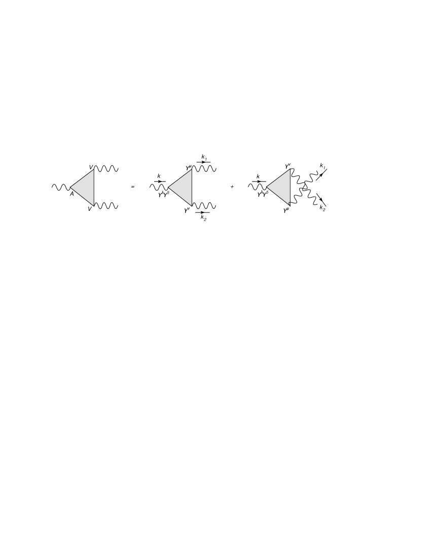
Figure 1: The ${\bf AVV}$ diagrams

Figure 2: The ${\bf AAA}$ diagrams

Its couplings are summarized in Tables 2 and 2, where “S” refers to the presence of a Stückelberg mass term for the corresponding gauge boson, if present. We have indicated, in this and in the model below, with a small lowercase (i.e. $b$ and $c$) the corresponding axions. The $U(1)_{A}$ symmetry is unbroken while $B$ gets its mass by the combined Higgs-Stückelberg mechanism. Another feature of the model, as we are going to see, is the presence of an Higgs-axion mixing generated not by a scalar potential (such as $V(\phi,b)$), as we will show in other examples, but by the fact that both mechanisms communicate their mass to the same gauge boson $B$. The axion remains a massless field in this case.

	A	B
$\psi$	$q^{A}_{L}=q^{A}_{R}=1$	$q^{B}_{R}=-q^{B}_{L}=1$

Table 1: Fermion assignments, A-B Model

	$\phi$	$S$
$A$	$q^{A}=0$	$0$
$B$	$q^{B}=-2$	$b$

Table 2: Gauge structure, A-B Model

Our discussion relies on the formalism of the 1-loop effective action, which is the generating functional of the one-particle irreducible correlation functions of a given model. The correlators are multiplied by external classical fields and the formalism allows to derive quite directly the anomalous Ward identities of the theory. The reader can find a discussion of the formalism in the appendix, where we study the properties of the Chern-Simons and Wess Zumino vertices of the model and their gauge variations.

In the A-B model, this will involve the classical defining action plus the anomaly diagrams with fermionic loops and we will require its invariance under gauge transformations. The structure of the (total) effective action is summarized, in the case of, say, one vector ($A$) and one axial vector ($B$) interaction by an expansion of the form

$$W[A,B] = \sum^{\infty}_{n_{1}=1}\sum^{\infty}_{n_{2}=1}\frac{i^{\,n_{1}+n_{2}}}{n_{1}!n_{2}!}\int dx_{1}...dx_{n_{1}}dy_{1}...dy_{n_{2}}T^{\lambda_{1}...\lambda_{n_{1}}\mu_{1}...\mu_{n_{2}}}(x_{1}...x_{n_{1}},y_{1}...y_{n_{2}})$$ (12)

$$\hskip 99.58464ptB^{\lambda_{1}}(x_{1})...B^{\lambda_{n_{1}}}(x_{n_{1}})A_{\mu_{1}}(y_{1})...A_{\mu_{n_{2}}}(y_{n_{2}}),$$

corresponding to the diagrams in Fig. 3

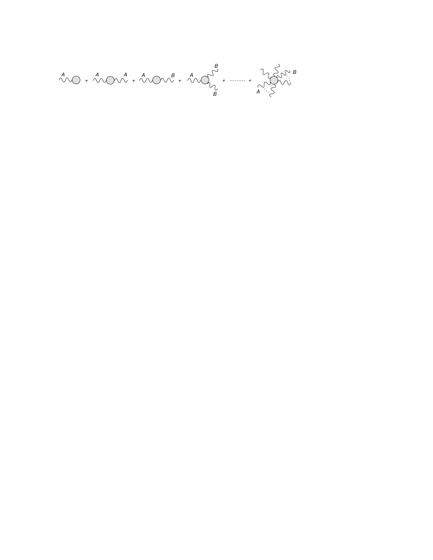
Figure 3: Expansion of the effective action

where we sum, for each diagram, over the symmetric exchanges of all the indices (including the momentum) of the identical gauge bosons (see also Fig. 4). As we are going to discuss next, also higher order diagrams of the form, for instance, AVVV will be affected by the presence of an undetermined shift in the triangle amplitudes, amounting to Chern-Simons interactions (CS). They turn to be well-defined once the distribution of the anomaly on 3-point functions is performed according to the correct Bose symmetries of these correlators of lower order.

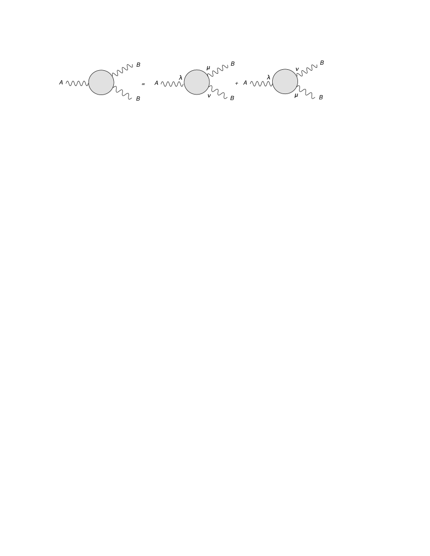
Figure 4: Triangle diagrams with permutations

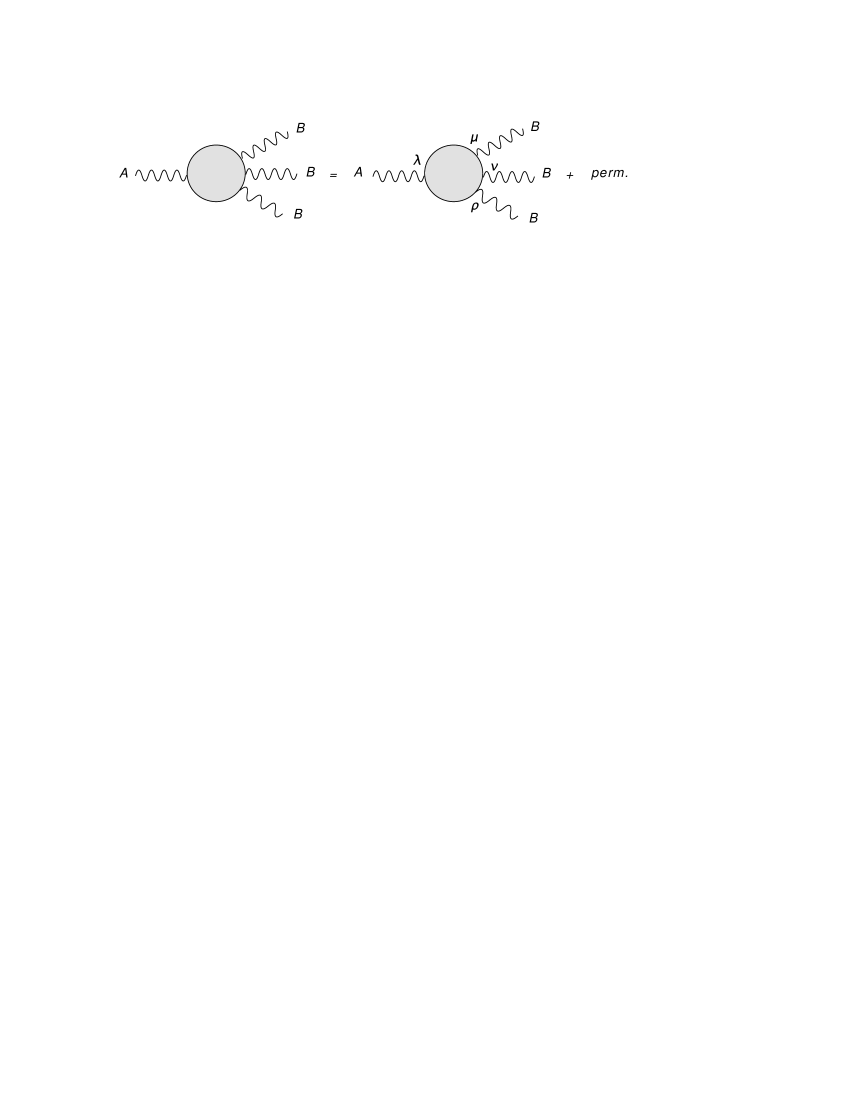
Figure 5: Symmetric expansion

Computing the variation of the generating functional we obtain

$$\delta_{B}W^{an}[A,B] = \frac{1}{2!}\int dxdydz\,T^{\lambda\mu\nu}(z,x,y)\,\delta B_{\lambda}(z)A_{\mu}(x)A_{\nu}(y)$$ (13)

$$+\frac{1}{3!}\int dxdydzdw\,T^{\lambda\mu\nu\rho}(z,x,y,w)B_{\lambda}(z)A_{\mu}(x)A_{\nu}(y)A_{\rho}(w),$$

using $\delta B_{\lambda}(z)=\partial_{\mu}\theta_{B}(z)$ and integrating by parts we get

$$\delta_{B}W^{an}[A,B] = -\frac{1}{2!}\int dxdydz\,\frac{\partial}{\partial z^{\lambda}}T^{\lambda\mu\nu}(z,x,y)\,\theta_{B}(z)A_{\mu}(x)A_{\nu}(y)$$

$$-\frac{1}{3!}\int dxdydzdw\,\frac{\partial}{\partial z^{\lambda}}T^{\lambda\mu\nu\rho}(z,x,y,w)\,\theta_{B}(z)A_{\mu}(x)A_{\nu}(y)A_{\rho}(w).$$

Notice that in configuration space the 4- and the 3- point function correlators are related by

$$\frac{\partial}{\partial z^{\lambda}}\overline{T}^{\lambda\mu\nu\rho}(z,x,y,w)=\delta(z-w)\overline{T}^{\rho\mu\nu}(w,x,y,)-\delta(z-x)\overline{T}^{\mu\nu\rho}(x,y,w)\mbox{+ perm.}$$ (15)

For $T$ we will be using the same conventions as for $\Delta$, with $\overline{T}^{\lambda\mu\nu}$ indicating a single diagram with non-permuted external gauge lines, while $T^{\lambda\mu\nu}$ will denote the symmetrized one (in $\mu\nu$). Clearly, the 1-loop effective theory of this model contains anomalous interactions that need to be cured by the introduction of suitable compensator fields. The role of the axions ($b$, for instance) is to remove the anomalies associated to the triangle diagrams which are correlators of 1 and 3 chiral currents respectively

$$T^{(\bf AVV)}_{\lambda\mu\nu}(x,y,z)=\langle 0|T\left(J_{\mu}(x)J_{\nu}(y)J^{5}_{\lambda}(z)\right)|0\rangle$$ (16)

and

$$T^{(\bf AAA)}_{\lambda\mu\nu}(x,y,z)=\langle 0|T\left(J^{5}_{\mu}(x)J^{5}_{\nu}(y)J^{5}_{\lambda}(z)\right)|0\rangle,$$ (17)

where

$$J_{\mu}=-\overline{\psi}\gamma_{\mu}\psi\qquad J^{5}_{\mu}=-\overline{\psi}\gamma_{\mu}\gamma_{5}\psi.$$ (18)

We denote by $\Delta(k_{1},k_{2})$ and $\Delta_{3}(k_{1},k_{2})$ their corresponding expressions in momentum space

$$(2\pi)^{4}\delta(k-k_{1}-k_{2})\Delta^{\lambda\mu\nu}(k_{1},k_{2})=\int dx\,dy\,dz\,e^{ik_{1}\cdot x+ik_{2}\cdot y-ik\cdot z}\,T^{\lambda\mu\nu}_{(\bf AVV)}(x,y,z)$$ (19)

$$(2\pi)^{4}\delta(k-k_{1}-k_{2})\Delta_{3}^{\lambda\mu\nu}(k_{1},k_{2})=\int dx\,dy\,dz\,e^{ik_{1}\cdot x+ik_{2}\cdot y-ik\cdot z}\,T^{\lambda\mu\nu}_{(\bf AAA)}(x,y,z).$$ (20)

Another point to remark is that the invariant amplitudes linear in momenta in the definition of the AVV trangle diagram correspond, in configuration space, to Chern-Simons interactions. In momentum space these are proportional to

$$V_{CS}^{\lambda\mu\nu}(k_{1},k_{2})=-i\epsilon^{\lambda\mu\nu\sigma}(k_{1}^{\sigma}-k_{2}^{\sigma})$$ (21)

and we denote with $T_{CS}^{\lambda\mu\nu}$ the corresponding contribution to the effective lagrangian in Minkowski space (see the appendices)

$$\mathcal{L}_{CS,ABA}=\int dxA^{\mu}(x)B^{\nu}(x)F_{A}^{\rho\sigma}(x)\varepsilon_{\mu\nu\rho\sigma}.$$ (22)

Moving to the anomalous part of the effective action, this takes the form, for generic gauge bosons $A_{i}$

$$\mathcal{S}_{eff}=\mathcal{S}_{0}+\mathcal{S}_{1},$$ (23)

where

$$\mathcal{S}_{1}=\sum_{i\,j\,k}\frac{1}{n_{i}!n_{j}!n_{k}!}g_{ijk}\int dxdydzA_{i}^{\lambda}(x)A_{j}^{\mu}(y)A_{k}^{\nu}(z)T^{\lambda\mu\nu}_{A_{i}A_{j}A_{k}}(x,y,z),$$ (24)

and where $A_{i}$ indicates an $A$ or a $B$ gauge boson, while $g_{ijk}$ is a short-hand notation for the product of the 3 coupling constants $g_{A_{i}}g_{A_{j}}g_{A_{k}}$, with an additional normalization due to a counting of identical external gauge bosons $(n_{i}!)$. All the anomalous contributions are included in the definition. In order to derive its explicit structure in our simplified cases, we consider the case of the $BAA$ vertex, the other examples being similar. We have, for instance, the partial contribution

$$\mathcal{S}^{BAA}=g_{B}\int dxdydzB_{\lambda}(z)\langle J_{5}^{\lambda}(z)e^{ig_{A}\int d^{4}xJ^{\mu}(x)A_{\mu}(x)}\rangle,$$ (25)

where the gauge fields are treated as classical fields and $\langle,\rangle$ indicate the vacuum expectation value. Expanding to second order, we keep only the connected contributions obtaining for instance

$$\mathcal{S}^{BAA}=\frac{i^{2}}{2!}g_{B}g_{A}^{2}\int dxdydzB_{\lambda}(z)A_{\mu}(x)A_{\nu}(y)\langle J_{5}^{\lambda}(z)J^{\mu}(x)J^{\nu}(y)\rangle.$$ (26)

This expresssion is our starting point for all the further analysis. Most of the manipulations concerning the proof of gauge-invariance of the effective action are more easily worked out in this formalism. Moving from momentum space to configuration space and back, may also be quite useful in order to detail the Ward identities of a given anomalous effective action.

In the presence of spontaneous symmetry breaking and of Stückelberg mass terms one has to decide whether the linear mixing between the Stückelberg field and the gauge boson is kept or not. One can keep the mixing and derive ordinary Ward identities for a given model. This is a possibility which is clearly at hand and can be useful. The disadvantage of this approach is that there is no gauge fixing parameter that can be used to analyze the gauge dependence of a given set of amplitudes and their cancelation. When the mixing is removed by going to a $R_{\xi}$ gauge, one can identify the set of gauge-invariant contributions to a given amplitude and identify more easily the conditions under which a given model becomes unitary. We follow this second approach. We are then able to combine gauge-dependent contributions in such a way that the unphysical poles of a given amplitude cancel. The analysis that we perform is limited to the s-channel, but the results are easily generalizable to the $t$ and $u$ channels as well. From this simple analysis one can easily extract information on the perturbative expansion of the effective action.

3.1 The anomalous effective Action of the $A-B$ Model

We start from the simplest model. In the $A-B$ model, defined in Eq. (11), the contribution to the anomalous effective action is given by

$$\mathcal{S}_{an} = \mathcal{S}_{1}+\mathcal{S}_{3}$$

$$\mathcal{S}_{1} = \int dx\,dy\,dz\,\left(\frac{g_{B}\,g^{2}_{A}}{2!}\,T_{\bf AVV}^{\lambda\mu\nu}(x,y,z)B_{\lambda}(z)A_{\mu}(x)A_{\nu}(y)\right)$$

$$\mathcal{S}_{3} = \int dx\,dy\,dz\,\left(\frac{g^{3}_{B}}{3!}\,T_{\bf AAA}^{\lambda\mu\nu}(x,y,z)B_{\lambda}(z)B_{\mu}(x)B_{\nu}(y)\right),$$

where we have collected all the anomalous diagrams of the form (AVV and AAA). We can easily express the gauge transformations of $A$ and $B$ in the form

$$\frac{1}{2!}\delta_{B}\langle T_{\bf AVV}BAA\rangle = \frac{i}{2!}a_{3}(\beta)\frac{1}{4}\langle F_{A}\wedge F_{A}\theta_{B}\rangle$$

$$\frac{1}{3!}\delta_{B}\langle T_{\bf AAA}BBB\rangle = \frac{i}{3!}\frac{a_{n}}{3}\frac{3}{4}\langle F_{B}\wedge F_{B}\theta_{B}\rangle,$$ (28)

where we have left open the choice over the parameterization of the loop momentum, denoted by the presence of the arbitrary parameter $\beta$ with

$$a_{3}(\beta)=-\frac{i}{4\pi^{2}}+\frac{i}{2\pi^{2}}\beta\qquad a_{3}\equiv\frac{a_{n}}{3}=-\frac{i}{6\pi^{2}},$$ (29)

while

$$\frac{1}{2!}\delta_{A}\langle T_{\bf AVV}BAA\rangle=\frac{i}{2!}a_{1}(\beta)\frac{2}{4}\langle F_{B}\wedge F_{A}\theta_{A}\rangle.$$ (30)

We have the following equations for the anomalous variations of the effective lagrangean

$$\delta_{B}\mathcal{L}_{an} = \frac{ig_{B}g^{\,2}_{A}}{2!}\,a_{3}(\beta)\frac{1}{4}F_{A}\wedge F_{A}\theta_{B}+\frac{ig^{\,3}_{B}}{3!}\,\frac{a_{n}}{3}\frac{3}{4}F_{B}\wedge F_{B}\theta_{B}$$

$$\delta_{A}\mathcal{L}_{an} = \frac{ig_{B}g^{\,2}_{A}}{2!}\,a_{1}(\beta)\frac{2}{4}F_{B}\wedge F_{A}\theta_{A},$$ (31)

while $\mathcal{L}_{b,c}$, the axionic contributions (Wess-Zumino terms), needed to restore the gauge symmetry violated at 1-loop level, are given by

$$\mathcal{L}_{b}=\frac{C_{AA}}{M}b\,F_{A}\wedge F_{A}+\frac{C_{BB}}{M}b\,F_{B}\wedge F_{B}.$$ (32)

Notice that since the axion shifts only under a gauge variation of the anomalous U(1) gauge field B (and not under A), gauge invariance of the effective action under a gauge transformation of the gauge field $A$ requires that

$$\delta_{A}\mathcal{L}_{an}=0.$$ (33)

Clearly, this condition fixes $\beta=-1/2\equiv\beta_{0}$ and is equivalent to the CVC condition on A that we had relaxed at the beginning. Imposing gauge invariance under B gauge transformations, on the other hand, we obtain

$$\delta_{B}\left(\mathcal{L}_{b}+\mathcal{L}_{an}\right)=0$$

which implies

$$C_{AA}=\frac{i\,g_{B}g^{\,2}_{A}}{2!}\frac{1}{4}\,a_{3}(\beta_{0})\,\frac{M}{M_{1}},\qquad C_{BB}=\frac{ig^{\,3}_{B}}{3!}\frac{1}{4}\,a_{n}\,\frac{M}{M_{1}}.$$ (35)

These conditions on the coefficients $C$ are sufficient to render gauge-invariant the total lagrangean. We observe that the presence of an abelian symmetry which has to remain exact and is not accompanied by a shifting axion has important implications on the consistency of the theory. We have brought up this example because in more complex situations in which a given gauge symmetry is broken and the pattern of breakings is such to preserve a final symmetry (for instance $U(1)_{em}$), the structure of the anomalous correlators, in some case, is drastically constrained to assume the CVC form. However this is not a general result.

Under a more general assumption, we could have allowed some Chern-Simons contributions in the counterterm lagrangean. This is an interesting variation that can be worked out at a diagrammatic level in order to identify the role played by the CS interactions. We will get back to this point once we start our diagrammatic analysis of these simple models.

4 Higgs-Axion Mixing in $U(1)$ Models: massless axi-Higgs

Having discussed how to render consistent to all orders the effective action, we need to discuss the role played by the shifting axions in the spectrum of the theory. We have already pointed out that the axion will mix with the remaining scalars of the model. In the presence of a Higgs sector such a mixing can take place at the level of the scalar potential, with drastic implications on the mass and the coupling of the axion to the remaining particles of the model. Naturally, one would like to understand the way the mixing occurs and this is exemplified in the case of the $AB$ model.

This model has two scalars: the Higgs and the Stückelberg fields. We assume that the Higgs field takes a non-zero vev and, as usual, the scalar field is expanded around the minimum $v$

$$\phi=\frac{1}{\sqrt{2}}\left(v+\phi_{1}+i\phi_{2}\right),$$ (36)

while from the quadratic part of the lagrangean we can easily read out the mass terms and the goldstone modes present in the spectrum in the broken phase. This is given by

$$\mathcal{L}_{q} = \frac{1}{2}\left(\partial_{\mu}\phi_{1}\right)^{2}+\frac{1}{2}\left(\partial_{\mu}\phi_{2}\right)^{2}+\frac{1}{2}\left(\partial_{\mu}b\right)^{2}+\frac{1}{2}\left(M_{1}^{2}+(q_{B}g_{B}v)^{2}\right)B_{\mu}B^{\mu}-\frac{1}{2}m_{1}^{2}\phi_{1}^{2}$$ (37)

$$+B_{\mu}\partial^{\mu}\left(M_{1}b+vg_{B}q_{B}\phi_{2}\right),$$

from which, after diagonalization of the mass terms we obtain

$$\mathcal{L}_{q} = \frac{1}{2}\left(\partial_{\mu}\chi_{B}\right)^{2}+\frac{1}{2}\left(\partial_{\mu}G_{B}\right)^{2}+\frac{1}{2}\left(\partial_{\mu}h_{1}\right)^{2}+\frac{1}{2}M_{B}^{2}B_{\mu}B^{\mu}-\frac{1}{2}m_{1}^{2}h_{1}^{2}$$ (38)

$$+M_{B}B^{\mu}\partial_{\mu}G_{B}$$

where we have redefined $\phi_{1}(x)=h_{1}(x)$ and $m_{1}=v\sqrt{2\lambda}$, for the Higgs field and its mass. We have identified the linear combinations

$$\chi_{B} = \frac{1}{M_{B}}\left(-M_{1}\,\phi_{2}+q_{B}g_{B}v\,b\right),$$

$$G_{B} = \frac{1}{M_{B}}\left(q_{B}g_{B}v\,\phi_{2}+M_{1}\,b\right),$$ (39)

corresponding to a massless particle, the axi-Higgs $\chi_{B}$, and a massless goldstone mode $G_{B}$. The rotation matrix that allows the change of variables $(\phi_{2},b)\to(\chi_{B},G_{B})$ is given by

$$U=\left(\begin{array}[]{ll}-\cos\theta_{B}&\sin\theta_{B}\\ \sin\theta_{B}&\cos\theta_{B}\end{array}\right)$$ (40)

with $\theta_{B}={\arccos}({M_{1}/M_{B}})={\arcsin}(q_{B}g_{B}v/M_{B})$. The axion $b$ can be expressed as linear combination of the rotated fields $\chi_{B}$,$G_{B}$ as

$$b=\alpha_{1}\chi_{B}+\alpha_{2}G_{B}=\frac{q_{B}g_{B}v}{M_{B}}\chi_{B}+\frac{M_{1}}{M_{B}}G_{B},$$ (41)

while the gauge fields $B_{\mu}$ get its mass $M_{B}$ through the combined Higgs-Stückelberg mechanism

$$M_{B}=\sqrt{M_{1}^{2}+(q_{B}g_{B}v)^{2}}.$$ (42)

To remove the mixing between the gauge fields and the goldstones we work in the $R_{\xi}$ gauge. The gauge-fixing lagrangean is given by

$$\mathcal{L}_{gf}=-\frac{1}{2}\mathcal{G}_{B}^{2}$$ (43)

where

$$\mathcal{G}_{B}=\frac{1}{\sqrt{\xi_{B}}}\left(\partial\cdot B-\xi_{B}M_{B}G_{B}\right),$$ (44)

and the corresponding ghost lagrangeans

$$\mathcal{L}_{B\,gh} = \overline{c_{B}}\left(-\square-\xi_{B}v_{u}(h_{1}+v_{u})-\xi_{B}M_{1}^{2}\right)c_{B}.$$ (45)

For convenience we report the form of the full lagrangean in the physical basis for future reference. After diagonalization of the mass matrix this becomes

$$\mathcal{L} = -\frac{1}{4}F_{A}^{2}-\frac{1}{4}F_{B}^{2}+\mathcal{L}_{Bgh}+\mathcal{L}_{f}+\mathcal{L}_{B}$$ (46)

where

$$\mathcal{L}_{B} = \frac{1}{2}\left(\partial_{\mu}\chi\right)^{2}-\frac{1}{2\xi_{B}}(\partial\cdot B)^{2}+\frac{1}{2}(\partial_{\mu}G_{B})^{2}+\frac{1}{2}(\partial_{\mu}h_{1})^{2}-\frac{1}{2}m_{1}^{2}h_{1}^{2}+\frac{1}{2}M_{B}^{2}B_{\mu}^{2}-4\frac{vg_{B}^{2}}{M_{B}}B_{\mu}G_{B}\partial^{\mu}h_{1}$$

$$-\frac{4\lambda v^{4}g_{B}^{4}}{M_{B}^{4}}G_{B}^{4}+\frac{8v^{2}g_{B}^{4}}{M_{B}^{2}}(B_{\mu})^{2}G_{B}^{2}+\frac{8\lambda M_{1}v^{3}g_{B}^{3}}{M_{B}^{4}}\chi_{B}G_{B}^{3}-\frac{8M_{1}vg_{B}^{3}}{M_{B}^{2}}(B_{\mu})^{2}\chi_{B}G_{B}$$

$$-\frac{4g_{B}^{2}\lambda v^{3}}{M_{B}^{2}}G_{B}^{2}h_{1}+4g_{B}^{2}(B_{\mu})^{2}h_{1}v+2\frac{g_{B}^{2}M_{1}^{2}}{M_{B}^{2}}(B_{\mu})^{2}\chi^{2}+2g_{B}^{2}(B_{\mu})^{2}h_{1}^{2}\frac{vg_{B}^{2}}{M_{B}}B_{\mu}h_{1}\partial^{\mu}G_{B}$$

$$+\frac{2\lambda M_{1}vg_{B}}{M_{B}^{2}}\chi G_{B}h_{1}^{2}+\frac{2g_{B}\lambda M_{1}^{3}v}{M_{B}^{4}}G_{B}\chi^{3}+\frac{4g_{B}\lambda M_{1}v^{2}}{M_{B}^{2}}G_{B}h_{1}\chi_{B}-\frac{2g_{B}M_{1}}{M_{B}}B^{\mu}\partial_{\mu}\chi h_{1}$$

$$-\frac{\lambda M_{1}^{4}}{4M_{B}^{4}}\chi^{4}+\frac{2g_{B}M_{1}}{M_{B}}B^{\mu}\partial_{\mu}h_{1}\chi_{B}-\frac{1}{4}\lambda h_{1}^{4}-\lambda vh_{1}^{3}+\frac{3\lambda M_{1}^{4}}{2M_{B}^{4}}\chi^{2}G_{B}^{2}-\frac{3\lambda M_{1}^{2}}{2M_{B}^{2}}\chi^{2}G_{B}^{2}$$

$$-\frac{1}{2}\lambda h_{1}^{2}G_{B}^{2}-\frac{1}{2}M_{B}^{2}\xi_{B}G_{B}^{2}-\frac{\lambda M_{1}^{2}}{2M_{B}^{2}}\chi^{2}h_{1}^{2}+\frac{\lambda M_{1}^{2}}{2M_{B}^{2}}G_{B}^{2}h_{1}^{2}-\frac{\lambda M_{1}^{2}v}{M_{B}^{2}}\chi^{2}h_{1}$$

where $\mathcal{L}_{f}$ denotes the fermion contribution.

At this stage there are some observations to be made. In the Stückelberg phase the axion $b$ is a goldstone mode, since it can be set to vanish by a gauge transformation on the B gauge boson, while $B$ is massive (with a mass $M_{1}$) and has 3 degrees of freedom (dof). Therefore in this phase the number of physical dof’s is 3 for $B$, 2 for $A$, 2 for the complex scalar Higgs $\phi$, for a total of 7. After electroweak symmetry breaking we have 3 d.o.f.’s for $B$, 2 for $A$ which remains massless in this model, 1 real Higgs field $h_{1}$ and 1 physical axion $\chi$, for a total of 7. The axion, in this case, on the contrary of what happens in the case of ordinary symmetry breaking is a massless physical scalar, being not part of the scalar potential. Not much surprise so far. Let’s now move to the analysis of the case when the axion is part of the scalar potential. In this second case the physical axion (the axi-Higgs) gets its mass by the combined Higgs-Stückelberg mechanisms and shows some interesting features.

4.1 Higgs-Axion Mixing in $U(1)$ Models: massive axi-Higgs

We now illustrate the mechanism of mass generation for the physical axion $\chi$. We focus on the breaking of the $U(1)_{B}$ gauge symmetry of the $AB$ model. We have a gauge-invariant Higgs potential given by

$$V_{PQ}=\mu^{2}\phi^{*}\phi+\lambda\left(\phi^{*}\phi\right)^{2}$$ (48)

plus the new PQ-breaking terms, allowed by the symmetry [19]

$$V_{P\hskip-6.0pt/\hskip 6.0ptQ\hskip-6.0pt/\hskip 6.0pt}=b_{1}\left(\phi\,e^{-iq_{B}g_{B}\frac{b}{M_{1}}}\right)+\lambda_{1}\left(\phi\,e^{-iq_{B}g_{B}\frac{b}{M_{1}}}\right)^{2}+2\lambda_{2}\left(\phi^{*}\phi\right)\left(\phi\,e^{-iq_{B}g_{B}\frac{b}{M_{1}}}\right)+\mbox{c.c.}$$ (49)

so that the complete potential considered is given by

$$V(H,b)=V_{PQ}+V_{P\hskip-6.0pt/\hskip 6.0ptQ\hskip-6.0pt/\hskip 6.0pt}+V^{*}_{P\hskip-6.0pt/\hskip 6.0ptQ\hskip-6.0pt/\hskip 6.0pt}.$$ (50)

We require that the minima of the potential are located at

$$\langle b\rangle=0\qquad\langle\phi\rangle=v,$$ (51)

which imply that the mass parameter satisfies

$$\mu^{2}=-\frac{b_{1}}{v}-2v^{2}\lambda-2\lambda_{1}-6v\lambda_{2}.$$ (52)

We are interested in the matrix describing the mixing of the CP-odd Higgs sector with the axion field $b$, given by

$$\left(\,\,\,\phi_{2},\,\,\,b\,\,\,\right){\mathcal{M}_{2}}\left(\begin{array}[]{c}\phi_{2}\\ b\end{array}\right)$$ (55)

where $\mathcal{M}_{2}$ is a symmetric matrix

$$\mathcal{M}_{2}=-\frac{1}{2}c_{\chi}v^{2}\pmatrix{1&-v\frac{q_{B}g_{B}}{M_{1}}\cr-v\frac{q_{B}g_{B}}{M_{1}}&v^{2}\frac{q^{2}_{B}g^{2}_{B}}{M^{2}_{1}}\cr}$$ (56)

and where the dimensionless coefficient multiplied in front is given by

$$c_{\chi}=4\left(\frac{b_{1}}{v^{3}}+\frac{4\lambda_{1}}{v^{2}}+\frac{2\lambda_{2}}{v}\right).$$ (57)

Notice that this parameter plays an important role in establishing the size of the mass of the physical axion, after diagonalization. It encloses all the dependence of the mass from the PQ corrections to the standard Higgs potential. They can be regarded as corrections of order $p/v$, with $p$ being any parameter of the PQ potential. If $p$ is very small, which is the case if the $V_{P\hskip-6.0pt/\hskip 6.0ptQ\hskip-6.0pt/\hskip 6.0pt}$ term of the potential is generated non-perturbatively (for instance by instanton effects in the case of QCD), the mass of the axi-Higgs can be pushed far below the typical mass of the electroweak breaking scenario (the Higgs mass), as discussed in [12].

The mass matrix has 1 zero eigenvalue corresponding to the goldstone boson G and 1 non-zero eigenvalue corresponding to a physical axion field $-\chi-$ with mass

$$m^{2}_{\chi}=-\frac{1}{2}c_{\chi}v^{2}\left[1+\frac{q^{2}_{B}g^{2}_{B}v^{2}}{M^{2}_{1}}\right]=-\frac{1}{2}c_{\chi}\,v^{2}\,\frac{M^{2}_{B}}{M^{2}_{1}}.$$ (58)

The mass of this state is positive if $c_{\chi}<0$. The rotation matrix that takes from the interaction eigenstates to the mass eigenstates is denoted by $O^{\chi}$

$$\left(\begin{array}[]{c}\chi\\ G\end{array}\right)=O^{\chi}\left(\begin{array}[]{c}\phi_{2}\\ b\end{array}\right)$$ (63)

so that we obtain the rotations

$$\phi_{2} = \frac{1}{M_{B}}(-M_{1}\,\chi+q_{B}g_{B}\,v\,G)$$ (64)

$$b = \frac{1}{M_{B}}(q_{B}g_{B}\,v\,\chi+M_{1}\,G).$$ (65)

The mass squared matrix can be diagonalized as

$$(\,\,\chi,\,G\,\,)O^{\chi}\,{\mathcal{M}_{2}}(O^{\chi})^{T}\left(\begin{array}[]{c}\chi\\ G\end{array}\right)=(\,\,\chi,\,G\,\,)\pmatrix{m^{2}_{\chi}&0\cr 0&0\cr}\left(\begin{array}[]{c}\chi\\ G\end{array}\right)$$ (70)

so that G is a massless goldstone mode and $m_{\chi}$ is the mass of the physical axion. In [12] one can find a discussion of some physical implications of this field when its mass is driven to be small in the instanton vacuum, similarly to the Peccei-Quinn axion of a global symmetry. However, given the presence of both mechanisms, the Stückelberg and the Higgs, it is not possible to decide whether this axion can be a valid dark-matter candidate. In the same work it is shown that the entire Stückelberg mechanism can be the result of a partial decoupling of a chiral fermion.

5 Unitarity issues in the A-B model in the exact phase

In this section we start discussing the issue of unitarity of the model that we have introduced. This is a rather involved topic that can be addressed by a diagrammatic analysis of those Feynman amplitudes with s-channel exchanges of gauge particles, the axi-Higgs and the NG modes, generated in the various phases of the theory (before and after symmetry breaking, with/without Yukawa couplings). The analysis could, of course, be repeated in the other channels (t,u) as well, but no further condition would be obtained. We will gather all the information coming from the study of the S-matrix amplitudes to set constraints on the parameters of the model. We have organized our analysis as a case-by-case study verifying the cancelation of the unphysical singularities in the amplitude in all the phases of the theory, establishing also their gauge independence. This is worked out in the $R_{\xi}$ gauge so to make evident the disappearance of the gauge-fixing parameter in each amplitude. The scattering amplitudes are built out of two anomalous diagrams with s-channel exchanges of gauge dependent propagators, and in all the cases we are brought back to the analysis of a set of anomalous Ward identities to establish our results.

5.1 Unitarity and CS interactions in the $A-B$ model

The first point that we address in this section concerns the role played by the CS interactions in the unitarity analysis of simple s-channel amplitudes. This analysis clarifies that CS interactions can be included or kept separately from the anomalous vertices with no consequence. To show this, we consider the following modification on the $AB$ model, where the CS interactions are generically introduced as possible counterterms in the 1-loop effective action, which is given by

$${\mathcal{L}}={\mathcal{L}_{0}}+{\mathcal{L}_{GS}}+{\mathcal{L}_{CS}},$$ (71)

where ${\mathcal{L}_{0}}$ is already known from previous sections, but in particular we focus on the components

$${\mathcal{L}_{GS}}=\frac{C_{AA}}{M}bF_{A}\wedge F_{A}+\frac{C_{BB}}{M}bF_{B}\wedge F_{B}$$ (72)

and

$${\mathcal{L}_{CS}}=d_{1}B^{\mu}A^{\nu}F^{\rho\sigma}_{A}\epsilon_{\mu\nu\rho\sigma}\equiv d_{1}BA\wedge F^{A}.$$ (73)

Under an $A$-gauge transformation we have

$$\delta_{A}{\mathcal{L}}=\frac{d_{1}}{2}\,\theta_{A}F_{B}\wedge F_{A}+\frac{i}{2!}a_{1}(\beta)\frac{2}{4}\,\theta_{A}F_{B}\wedge F_{A},$$ (74)

so that we obtain

$$\frac{d_{1}}{2}+\frac{ia_{1}(\beta)}{4}=0\,\,\,\,\,\leftrightarrow\,\,\,\,\,d_{1}=-\frac{i}{2}a_{1}(\beta).$$ (75)

Analogously, under a $B$-gauge transformation we have

$$\delta_{B}{\mathcal{L}}=-\frac{d_{1}}{2}\theta_{B}F_{A}\wedge F_{A}+\frac{i}{2!}a_{3}(\beta)\frac{1}{4}F_{A}\wedge F_{A}\theta_{B}-C_{AA}\frac{M_{1}\theta_{B}}{M}\,F_{A}\wedge F_{A}$$

$$\,\,\,\,\,\,\,\,\,\,\,\,\,\,\,\,\,\,-C_{BB}\frac{M_{1}\theta_{B}}{M}F_{B}\wedge F_{B}+\frac{i}{3!}\frac{a_{n}}{3}\frac{3}{4}\theta_{B}F_{B}\wedge F_{B},$$ (76)

to obtain

$$-\frac{d_{1}}{2}-C_{AA}\frac{M_{1}}{M}+\frac{i}{2!}a_{3}(\beta)\frac{1}{4}=0\,\,\,\,\,\leftrightarrow\,\,\,\,\,C_{AA}=\left(-\frac{d_{1}}{2}+\frac{i}{2!}a_{3}(\beta)\frac{1}{4}\right)\frac{M}{M_{1}}.$$ (77)

Figure 6: Diagrams involved in the unitarity analysis with external CS interactions.

We refer the reader to one of the appendices where the computation is performed in detail.

We have shown that the presence of external Ward identities forcing the invariant amplitudes of a given anomalous triangle diagram to assume a specific form, allow to re-absorb the CS coefficients inside the triangle, thereby simplifyig the computations. In this specific case the CVC condition for $A$ is a property of the theory. In other cases this does not take place. For instance, instead of the condition $a_{1}(\beta)=0$, a less familiar condition such as $a_{3}(\beta)=0$ (conserved axial current, CAC) may be needed. In this sense, if we define the CVC condition to be the “standard case”, the CAC condition points toward a new anomalous interaction. We remark once more that $\beta$ remains “free” in the SM, since the anomaly traces cancel for all the generators, differently from this new situation. The theory allows new CS interactions, with the understanding that, at least in these cases, these interactions can be absorbed into a redefinition of the vertex. However, the presence of a Ward identity, that allows us to re-express $a_{1}$ and $a_{2}$ in terms of $a_{3}\dots a_{6}$ in different ways, at the same time allows us to come up with different gauge invariant expressions of the same vertex function (fixed by a CVC or a CAC condition, depending on the case). These different versions of these AVV 3-point functions are characterized by different (gauge-variant) contact interactions since $a_{1}$ and $a_{2}$ in Minkowski space contain, indeed, CS interactions. We will elaborate on this point in a following section where we discuss the structure of the effective action in Minkowski space.

The extension of this pattern to the broken Higgs phase can be understood from Fig. 7 where the additional contributions have been explicitly included. We have depicted the CS terms as separate contributions and shown perfect cancelation also in this case.

Figure 7: Unitarity issue for the AB model in the broken phase.

The complete set of diagrams is shown in Fig. (7)

$$S_{\xi}=A_{\xi}+B_{\xi}+C_{\xi}+D_{\xi}+E_{\xi}+F_{\xi}+G_{\xi}+H_{\xi}$$ (78)

and the total gauge dependence vanishes. Details can be found in the appendix.

6 Gauge independence of the A self-energy to higher orders and the loop counting

In this section we move to an analysis performed to higher orders that illustrates how the loop expansion and the counterterms get organized so to have a consistent gauge independent theory.

For this purpose, let’s consider the diagrams in Fig. 8, which are relevant in order to verify this cancelation in the massless fermion case. It shows the self-energy of the A gauge boson. From now on we are dropping all the coupling constants to simplify the notation, which can be re-inserted at the end. We have omitted diagrams which are symmetric with respect to the two intermediate lines of the B and A gauge bosons, for simplicity. This symmetrization is responsible for the cancelation of the gauge dependence of the propagator of $A$ and the vector interaction of B, while the gauge dependence of the axial-vector contribution of B is canceled by the corresponding goldstone (shown). Diagram (A) involves 3 loops and therefore we need to look for cancelations induced by a diagram involving the s-channel exchange both of an $A$ and of a $B$ gauge boson plus the 1-loop interactions involving the relevant counterterms. In this case one easily identifies diagram (B) as the only possible additional contribution.

To proceed with the demonstration we first isolate the gauge dependence in the propagator for the gauge boson exchanged in the s-channel

$$\frac{-i}{k^{2}-M_{1}^{2}}\left[g^{\,\lambda\,\lambda^{\prime}}-\frac{k^{\lambda}\,k^{\lambda^{\prime}}}{k^{2}-\xi_{B}M_{1}^{2}}(1-\xi_{B})\right] = \frac{-\,i}{k^{2}-M_{1}^{2}}\left(g^{\,\lambda\,\lambda^{\prime}}-\frac{k^{\lambda}\,k^{\lambda^{\prime}}}{M_{1}^{2}}\right)+\frac{-\,i}{k^{2}-\xi_{B}\,M_{1}^{2}}\left(\frac{k^{\lambda}k^{\lambda^{\prime}}}{M_{1}^{2}}\right)$$ (79)

$$= P_{0}^{\lambda\,\lambda^{\prime}}+P_{\xi}^{\lambda\,\lambda^{\prime}}.$$

Figure 8: 3 loop cancelations of the gauge dependence.

and using this separation, the sum involving the two diagrams gives

$$S=\int\frac{d^{4}k_{2}}{(2\pi)^{4}}({\mathcal{A}}+{\mathcal{B}}),$$ (80)

with the gauge-dependent contributions being given by

$${\mathcal{A}}_{\xi 0} = \,\Delta^{\lambda\mu\nu}(-k_{1},-k_{2})P^{\lambda\lambda^{\prime}}_{\xi}\Delta^{\lambda^{\prime}\mu^{\prime}\nu^{\prime}}(k_{1},k_{2})P^{\nu\nu^{\prime}}_{o}$$

$$= \,\Delta^{\lambda\mu\nu}(-k_{1},-k_{2})\left[\frac{-i}{k^{2}-\xi_{B}M^{2}_{1}}\left(\frac{k^{\lambda}k^{\lambda^{\prime}}}{M^{2}_{1}}\right)\right]\Delta^{\lambda^{\prime}\mu^{\prime}\nu^{\prime}}(k_{1},k_{2})\left[\frac{-ig^{\nu\nu^{\prime}}}{k^{2}_{2}}\right]$$

$${\mathcal{B}}_{\xi 0} = 4\times\left(\frac{4}{M}C_{AA}\right)^{2}\epsilon^{\,\mu\nu\rho\sigma}k_{1\rho}k_{2\sigma}\frac{i}{k^{2}-\xi_{B}M^{2}_{1}}\epsilon^{\,\mu^{\prime}\nu^{\prime}\rho^{\prime}\sigma^{\prime}}k_{1\rho^{\prime}}k_{2\sigma^{\prime}}P^{\nu\nu^{\prime}}_{o}.$$ (81)

Using the anomaly equations and substituting the appropriate value already obtained for the WZ-coefficient, we obtain a vanishing expression

$${\mathcal{A}}_{\xi 0}+{\mathcal{B}}_{\xi 0} = (-a_{3}(\beta)\epsilon^{\,\mu\nu\rho\sigma}k_{1\rho}k_{2\sigma})\left[\frac{-i}{k^{2}-\xi_{B}M^{2}_{1}}\frac{1}{M^{2}_{1}}\right](a_{3}(\beta)\epsilon^{\,\mu^{\prime}\nu^{\prime}\rho^{\prime}\sigma^{\prime}}k_{1\rho^{\prime}}k_{2\sigma^{\prime}})P^{\nu\nu^{\prime}}_{o}$$

$$+ 4\,\frac{16}{M^{2}}\left(\frac{i}{2!}\frac{1}{4}a_{3}(\beta)\frac{M}{M_{1}}\right)^{2}\epsilon^{\,\mu\nu\rho\sigma}k_{1\rho}k_{2\sigma}\frac{i}{k^{2}-\xi_{B}M^{2}_{1}}\epsilon^{\,\mu^{\prime}\nu^{\prime}\rho^{\prime}\sigma^{\prime}}k_{1\rho^{\prime}}k_{2\sigma^{\prime}}P^{\nu\nu^{\prime}}_{o}=0.$$

After symmetry breaking, with massive fermions, the pattern gets far more involved and is described in Fig. 9. Also in this case we have

Figure 9: The complete set of diagrams in the broken phase.

$$S=\int\frac{d^{4}k_{2}}{(2\pi)^{4}}({\mathcal{A}}+{\mathcal{B}}+{\mathcal{C}}+{\mathcal{D}}+{\mathcal{E}})$$ (83)

and it can be shown by direct computation that the gauge dependences cancel in this combination. The interested reader can find the discussion in the appendix (“Gauge cancelations in the self-energy diagrams”). Notice that the pattern to follow in order to identify the relevant diagrams is quite clear, and it is not difficult to identify at each order of the loop expansion contributions with the appropriate s-channel exchanges that combine into gauge invariant amplitudes. These are built identifying direct contributions and counterterms in an appropriate fashion, counting the counterterms at their appropriate order in Planck’s constant $(h)$. The identification of similar patterns in the broken phase is more cumbersome and is addressed below.

7 Unitarity Analysis of the AB model in the broken phase

In the broken phase and in the presence of Yukawa couplings there are some modifications that take place, since the s-channel exchange of the $b$ axion is rotated on the two components (the goldstone and physical axion $\chi$) as shown later in Fig. 12. The introduction of the Yukawa interaction and the presence of a symmetry breaking phase determines an interaction of the axion with the fermions. Therefore, let’s consider the Yukawa lagrangean

$${\cal{L}}_{Y}=-\lambda_{1}\,\overline{\psi}_{L}\phi\,\psi_{R}-\lambda_{1}\,\overline{\psi}_{R}\phi^{*}\psi_{L},$$ (84)

which is needed to extract the coupling between the axi-Higgs and the fermions. We focus on the term

$${\cal{L}}_{Y}(\phi_{2})=-\frac{\lambda_{1}}{2}\left[\overline{\psi}(1+\gamma^{5})\psi\,\frac{i\phi_{2}}{\sqrt{2}}-\overline{\psi}(1-\gamma^{5})\psi\,\frac{i\phi_{2}}{\sqrt{2}}\right],$$ (85)

having expanded around the Higgs vacuum. Performing a rotation to express the pseudoscalar Higgs phase $\phi_{2}$ in terms of the physical axion and the NG boson

$$\phi_{2}=-\frac{M_{1}}{M_{B}}\chi_{B}+\frac{q_{B}g_{B}v}{M_{B}}G_{B},$$

one extracts a $\chi\overline{\psi}\psi$ coupling of the kind

$${\cal{L}}_{Y}(\chi_{B})=\frac{\lambda_{1}}{\sqrt{2}}\frac{M_{1}}{M_{B}}i\,\overline{\psi}\chi_{B}\gamma^{5}\psi,$$ (86)

and a coupling $G\overline{\psi}\psi$ for the goldstone mode

$${\cal{L}}_{Y}(G_{B})=-\frac{\lambda_{1}}{\sqrt{2}}\frac{q_{B}g_{B}v}{M_{B}}i\,\overline{\psi}\,G_{B}\gamma^{5}\psi=2g_{B}\frac{m_{f}}{M_{B}}i\overline{\psi}\gamma^{5}\psi G_{B}.$$ (87)

Having fixed the Yukawa couplings of the model, we move to the analysis of the same diagrams of the previous section in the broken phase. Preliminarily, we need to identify the structure of the anomaly equation for the fermionic 3-point functions with their complete mass dependence. In the case of massive fermions the anomalous Ward identities for an AVV triangle are of the form

$$k_{1\mu}\Delta^{\lambda\mu\nu}(\beta,k_{1},k_{2}) = a_{1}(\beta)\varepsilon^{\lambda\nu\alpha\beta}k_{1}^{\alpha}k_{2}^{\beta},$$

$$k_{2\nu}\Delta^{\lambda\mu\nu}(\beta,k_{1},k_{2}) = a_{1}(\beta)\varepsilon^{\lambda\mu\alpha\beta}k_{2}^{\alpha}k_{1}^{\beta},$$

$$k_{\lambda}\Delta^{\lambda\mu\nu}(\beta,k_{1},k_{2}) = a_{3}(\beta)\varepsilon^{\mu\nu\alpha\beta}k_{1}^{\alpha}k_{2}^{\beta}+2m_{f}\Delta^{\mu\nu},$$ (88)

and in the case of AAA triangle $\Delta_{3}^{\lambda\mu\nu}(\beta,k_{1},k_{2})=\Delta_{3}^{\lambda\mu\nu}(k_{1},k_{2})$, with Bose symmetry providing a factor 1/3 for the distribution of the anomalies among the 3 vertices

$$k_{1\mu}\Delta_{3}^{\lambda\mu\nu}(k_{1},k_{2}) = \frac{a_{n}}{3}\varepsilon^{\lambda\nu\alpha\beta}k_{1}^{\alpha}k_{2}^{\beta}+2m_{f}\Delta^{\lambda\nu},$$

$$k_{2\nu}\Delta_{3}^{\lambda\mu\nu}(k_{1},k_{2}) = \frac{a_{n}}{3}\varepsilon^{\lambda\mu\alpha\beta}k_{2}^{\alpha}k_{1}^{\beta}+2m_{f}\Delta^{\lambda\mu},$$

$$k_{\lambda}\Delta_{3}^{\lambda\mu\nu}(k_{1},k_{2}) = \frac{a_{n}}{3}\varepsilon^{\mu\nu\alpha\beta}k_{1}^{\alpha}k_{2}^{\beta}+2m_{f}\Delta^{\mu\nu},$$ (89)

where we have dropped the appropriate coupling constants common to both sides. The amplitude $\Delta^{\mu\nu}$ is given by

$$\Delta^{\mu\nu}=\int\frac{d^{4}q}{(2\pi)^{4}}\frac{Tr\left[\gamma^{5}(q\hskip-6.0pt/\hskip 6.0pt-k\hskip-6.0pt/\hskip 6.0pt+m_{f})\gamma^{\nu}\gamma^{5}(q\hskip-6.0pt/\hskip 6.0pt-k\kern-4.30554pt\hbox{/}_{1}+m_{f})\gamma^{\mu}\gamma^{5}(q\hskip-6.0pt/\hskip 6.0pt+m_{f})\right]}{[q^{2}-m_{f}^{2}][(q-k)^{2}-m_{f}^{2}][(q-k_{1})^{2}-m_{f}^{2}]}\mbox{+ exch.}$$ (90)

and can be expressed as a two-dimensional integral using the Feynman parameterization. We find

$$\Delta^{\mu\nu} = \epsilon^{\alpha\beta\mu\nu}k_{1}^{\alpha}k_{2}^{\beta}m_{f}\left(\frac{1}{2\pi^{2}}\right)I,$$

with $I$ denoting the formal expression of the integral

$$I\equiv\int^{1}_{0}dx\int^{1-x}_{0}dy\frac{(1-2x-2y)}{\Delta(x,y,m_{f},m_{\chi},M_{B})}.$$ (92)

We have dropped the charge dependence since we have normalized the charges to unity and we have defined

$$\Delta(x,y,m_{f},m_{\chi},M_{B})=\Sigma^{2}-D=m_{f}^{2}-x\,y\,m_{\chi}^{2}+M_{B}^{2}(x+y)^{2}-xM_{B}^{2}-yM_{B}^{2}\equiv\Delta(x,y).$$ (93)

We can use this amplitude to compute the 1-loop decay of the axi-Higgs in this simple model, shown in Fig. 10, which is given by

$${\mathcal{M}}_{\chi\rightarrow BB} = {\mathcal{A}}+{\mathcal{B}}$$ (94)

$$= i\frac{\lambda_{1}}{\sqrt{2}}\frac{M_{1}}{M_{B}}\Delta^{\mu\nu}(k_{1},k_{2})+\alpha_{1}\frac{4}{M}C_{BB}$$

$$= i\frac{\lambda_{1}}{\sqrt{2}}\frac{M_{1}}{M_{B}}\Delta^{\mu\nu}(k_{1},k_{2})-\frac{2g_{B}v}{M_{B}}\left(\frac{4}{M}\frac{i}{3!}\frac{1}{4}a_{n}\frac{M}{M_{1}}\right),$$

where $\alpha_{1}$ is the coefficient that rotates the axion $b$ on the axi-higgs particle $\chi$. The related cross section is shown in Fig. 11.

Figure 10: Decay amplitude for $\chi\to BB$.

Figure 11: Decay cross section for $\chi\to BB$.

7.1 A-B model: BB $\rightarrow$ BB mediated by a B gauge boson in the broken phase

Figure 12: Diagrams from the Green-Schwarz coupling after symmetry breaking.

A second class of contributions that require a different distribution of the partial anomalies are those involving $BBB$ diagrams. They appear in the $BB\to BB$ amplitude, mediated by the exchange of a $B$ gauge boson of mass $M_{B}=\sqrt{M_{1}^{2}+(2g_{B}v)^{2}}$. Notice that $M_{B}$ gets its mass both from the Higgs and the Stückelberg sectors. The relevant diagrams for this check are shown in Fig. 13. We have not included the exchange of the physical axion, since this is not gauge-dependent. We are only after the gauge-dependent contributions. Notice that the expansion is valid at 2-loop level and involves 2-loop diagrams built as combinations of the original diagrams and of the 1-loop counterterms. There are some comments that are due in order to appreciate the way the cancelations take place. If we neglect the Yukawa couplings the diagrams (B), (C) and (D) are absent, since the goldstone does not couple to a massless fermion. In this case, the axion $b$ is rotated, as in the previous sections, into a goldstone mode $G_{B}$ and a physical axion $\chi$ (see Fig. 12). On the other hand, if we include the Yukawa couplings then the entire set of diagrams is needed.

Figure 13: Cancelation of the gauge dependence after spontaneous symmetry breaking.

From diagram (E) we obtain the partial contribution

$$\mathcal{E}_{\xi}=4\times\left(\frac{4}{M}\alpha_{2}C_{BB}\right)^{2}\varepsilon^{\mu\nu\rho\sigma}k_{1}^{\rho}k_{2}^{\sigma}\left(\frac{i}{k^{2}-\xi_{B}M_{B}^{2}}\right)\varepsilon^{\mu^{\prime}\nu^{\prime}\rho^{\prime}\sigma^{\prime}}k_{1}^{\rho^{\prime}}k_{2}^{\sigma^{\prime}},$$ (95)

where the overall factor of 4 in front is a symmetry factor, the coefficient $\alpha_{2}$ comes from the rotation of the b axion over the goldstone boson ($\alpha_{2}=\frac{M_{1}}{M_{B}}$), and the coefficient $C_{BB}$ has already been determined from the condition of gauge invariance of the anomalous effective action before symmetry breaking. Similarly, from diagram (B) we get the term

$$\mathcal{B}_{\xi}=(g_{B})^{3}\Delta^{\mu\nu}(-k_{1},-k_{2})\left(2i\,\frac{m_{f}}{M_{B}}\right)\frac{i}{k^{2}-\xi_{B}M_{B}^{2}}\left(2i\frac{m_{f}}{M_{B}}\right)(g_{B})^{3}\Delta^{\mu^{\prime}\nu^{\prime}}(k_{1},k_{2}),$$ (96)

while diagram (C) gives

$$\mathcal{C}_{\xi}=2\times(g_{B})^{3}\Delta^{\mu\nu}(-k_{1},-k_{2})\left(2\,i\frac{m_{f}}{M_{B}}\right)\frac{i}{k^{2}-\xi_{B}M_{B}^{2}}\left(\frac{4}{M}\alpha_{2}C_{BB}\,\varepsilon^{\mu^{\prime}\nu^{\prime}\rho^{\prime}\sigma^{\prime}}k_{1}^{\rho^{\prime}}k_{2}^{\sigma^{\prime}}\right),$$ (97)

having introduced also in this case a symmetry factor. Finally (D) gives

$$\mathcal{D}_{\xi}=2\times\left(\frac{4}{M}\alpha_{2}C_{BB}\varepsilon^{\mu\nu\rho\sigma}k_{1}^{\rho}k_{2}^{\sigma}\right)\frac{i}{k^{2}-\xi_{B}M_{B}^{2}}\left(2\,i\frac{m_{f}}{M_{B}}\right)\Delta^{\mu^{\prime}\nu^{\prime}}(k_{1},k_{2})(g_{B})^{3}.$$ (98)

We will be using the anomaly equation in the massive fermion case, having distributed the anomaly equally among the three B vertices

$$k^{\lambda}\Delta^{\lambda\mu\nu}=\frac{a_{n}}{3}\varepsilon^{\mu\nu\alpha\beta}k_{1}^{\alpha}k_{2}^{\beta}+2m_{f}\Delta^{\mu\nu}.$$ (99)

Separating in diagram (A) the gauge dependent part of the propagator of the boson B from the rest we obtain

$$\mathcal{A}_{\xi} = \Delta^{\lambda\mu\nu}\frac{-i}{k^{2}-\xi_{B}M_{B}^{2}}\left(\frac{k^{\lambda}k^{\lambda^{\prime}}}{M^{2}_{B}}\right)\Delta^{\lambda^{\prime}\mu^{\prime}\nu^{\prime}}$$ (100)

$$= \left(\frac{a_{n}}{3}\varepsilon^{\mu\nu\alpha\beta}k_{1}^{\alpha}k_{2}^{\beta}+2m_{f}\Delta^{\mu\nu}\right)(g_{B})^{3}\frac{i}{k^{2}-\xi_{B}M_{B}^{2}}\frac{1}{M_{B}^{2}}\left(\frac{a_{n}}{3}\varepsilon^{\mu^{\prime}\nu^{\prime}\alpha^{\prime}\beta^{\prime}}k_{1}^{\alpha^{\prime}}k_{2}^{\beta^{\prime}}+2m_{f}\Delta^{\mu^{\prime}\nu^{\prime}}\right)(g_{B})^{3}$$

$$= \frac{i}{k^{2}-\xi_{B}M_{B}^{2}}\frac{g^{\,6}_{B}}{M_{B}^{2}}\left[\left(\frac{a_{n}}{3}\right)^{2}\varepsilon^{\mu\nu\alpha\beta}\varepsilon^{\mu^{\prime}\nu^{\prime}\alpha^{\prime}\beta^{\prime}}k_{1}^{\alpha}k_{2}^{\beta}k_{1}^{\alpha^{\prime}}k_{2}^{\beta^{\prime}}\right.$$

$$\left.+\frac{a_{n}}{3}\varepsilon^{\mu\nu\alpha\beta}k_{1}^{\alpha}k_{2}^{\beta}\,2m_{f}\Delta^{\mu^{\prime}\nu^{\prime}}+2m_{f}\Delta^{\mu\nu}\frac{a_{n}}{3}\varepsilon^{\mu^{\prime}\nu^{\prime}\alpha^{\prime}\beta^{\prime}}k_{1}^{\alpha^{\prime}}k_{2}^{\beta^{\prime}}\right.$$

$$\left.+\left(2m_{f}\Delta^{\mu\nu}\right)(2m_{f}\Delta^{\mu^{\prime}\nu^{\prime}})\right].$$

The first term in (100) is exactly canceled by the contribution from diagram (E). The last contribution cancels by the contribution from diagram (B). Finally diagrams (C) and (D) cancel against the second and third contributions from diagram (A).

8 The effective action in the Y-B model

We anticipate in this section some of the methods that will be used in [25] in the analysis of a realistic model. In the previous model, in order to simplify the analysis, we have assumed that the coupling of the B gauge boson was purely axial while $A$ was purely vector-like. Here we discuss a gauge structure which allows both gauge bosons to have combined vector and axial-vector couplings. We will show that the external Ward identities of the model involve a specific definition of the shift parameter in one of the triangle diagrams that forces the axial-vector current to be conserved ($a_{3}(\beta)=0$). This result, new compared to the case of the SM, shows the presence of an effective CS term in some amplitudes.

The lagrangean that we choose to exemplify this new situation is given by

$${\mathcal{L}}_{0} = |(\partial_{\mu}+ig_{Y}q^{Y}_{u}Y_{\mu}+ig_{B}q^{B}_{u}B_{\mu})\phi_{u}|^{2}+|(\partial_{\mu}+ig_{Y}q^{Y}_{d}Y_{\mu}+ig_{B}q^{B}_{d}B_{\mu})\phi_{d}|^{2}-\frac{1}{4}F^{2}_{Y}-\frac{1}{4}F^{2}_{B}$$ (101)

$$+ \frac{1}{2}(\partial_{\mu}b+M_{1}B_{\mu})^{2}-\lambda_{u}\left(|\phi_{u}|^{2}-\frac{v_{u}}{2}\right)^{2}-\lambda_{d}\left(|\phi_{d}|^{2}-\frac{v_{d}}{2}\right)^{2}+{\mathcal{L}}_{f}+{\mathcal{L}}_{Yuk},$$

where the Yukawa couplings are given by

$${\mathcal{L}}_{Yuk}=-\lambda_{1}\overline{\psi}_{1L}\phi_{u}\psi_{1R}-\lambda_{1}\overline{\psi}_{1R}\phi^{*}_{u}\psi_{1L}-\lambda_{2}\overline{\psi}_{2L}\phi_{d}\psi_{2R}-\lambda_{2}\overline{\psi}_{2R}\phi^{*}_{d}\psi_{2L},$$ (102)

with $L$ and $R$ denoting left- and right- handed fermions.

The fermion currents are

$${\mathcal{L}}_{f} = \overline{\psi}_{1L}i\gamma^{\mu}\left[\partial_{\mu}+ig_{Y}q^{Y}_{1L}Y_{\mu}+ig_{B}q^{B}_{1L}B_{\mu}\right]\psi_{1L}+\overline{\psi}_{1R}i\gamma^{\mu}\left[\partial_{\mu}+ig_{Y}q^{Y}_{1R}Y_{\mu}+ig_{B}q^{B}_{1R}B_{\mu}\right]\psi_{1R}$$

$$+ \overline{\psi}_{2L}i\gamma^{\mu}\left[\partial_{\mu}+ig_{Y}q^{Y}_{2L}Y_{\mu}+ig_{B}q^{B}_{2L}B_{\mu}\right]\psi_{2L}+\overline{\psi}_{2R}i\gamma^{\mu}\left[\partial_{\mu}+ig_{Y}q^{Y}_{2R}Y_{\mu}+ig_{B}q^{B}_{2R}B_{\mu}\right]\psi_{2R}$$

so that, in general, without any particular charge assignment, both gauge bosons show vector and axial-vector couplings. In this case we realize an anomaly-free charge assignment for the hypercharge by requiring that $q^{Y}_{2L}=-q^{Y}_{1L},q^{Y}_{2R}=-q^{Y}_{1R}$, which cancels the anomaly for a YYY triangle since

$$\sum_{f=1,2}(q^{Y}_{f})^{3}=(q^{Y}_{1R})^{3}-(q^{Y}_{1L})^{3}+(q^{Y}_{2R})^{3}-(q^{Y}_{2L})^{3}=(q^{Y}_{1R})^{3}-(q^{Y}_{1L})^{3}-(q^{Y}_{1R})^{3}+(q^{Y}_{1L})^{3}=0.$$

This condition is similar to the vanishing of the (YYY) anomaly for the hypercharge in the SM, and for this reason we will assume that it holds also in our simplified model.

Before symmetry breaking the B gauge boson has a goldstone coupling coming from the Stückelberg mass term due to the presence of a Higgs field. The effective action for this model is given by

$${\mathcal{S}}_{eff}={\mathcal{S}}_{an}+{\mathcal{S}}_{WZ},$$ (105)

which reads

$${\mathcal{S}}_{an} = \frac{1}{3!}\langle T^{\lambda\mu\nu}_{BBB}(z,x,y)B^{\lambda}B^{\mu}B^{\nu}\rangle+\frac{1}{2!}\langle T^{\lambda\mu\nu}_{BYY}(z,x,y)B^{\lambda}Y^{\mu}Y^{\nu}\rangle+\frac{1}{2!}\langle T^{\lambda\mu\nu}_{YBB}(z,x,y)Y^{\lambda}B^{\mu}B^{\nu}\rangle$$

with

$${\mathcal{S}}_{WZ}=\frac{C_{YY}}{M}\,\langle b\,F^{Y}\wedge F^{Y}\rangle+\frac{C_{BB}}{M}\,\langle b\,F^{B}\wedge F^{B}\rangle+\frac{C_{BY}}{M}\,\langle b\,F^{B}\wedge F^{Y}\rangle$$ (107)

denoting the WZ counterterms. Only for the triangle BBB we have assumed an anomaly symmetrically distributed, all the other anomalous diagrams having an AVV anomalous structure, given in momentum space by

$$\Delta^{\lambda\mu\nu}_{ijk}=\frac{i^{3}}{2}\sum_{f}\left[q^{i}_{f}q^{j}_{f}q^{k}_{f}\right]\int\frac{d^{4}p}{(2\pi)^{4}}\frac{Tr[\gamma^{\lambda}\gamma^{5}p\hskip-6.0pt/\hskip 6.0pt\gamma^{\mu}(p\hskip-6.0pt/\hskip 6.0pt-k\kern-4.30554pt\hbox{/}_{1})\gamma^{\nu}(p\hskip-6.0pt/\hskip 6.0pt-k\kern-4.30554pt\hbox{/})]}{p^{2}(p-k_{1})^{2}(p-k)^{2}}+\{\mu,k_{1}\,\,\leftrightarrow\,\,\nu,k_{2}\},$$

with indices running over i, j, k =Y, B. The sum over the fermionic spectrum involves the charge operators in the chiral basis

$$D_{ijk}=\frac{1}{2}\sum_{f=1,2}\left[q^{i}_{f}q^{j}_{f}q^{k}_{f}\right]\equiv\frac{1}{2}\sum_{f}\left(q^{i}_{fR}q^{j}_{fR}q^{k}_{fR}-q^{i}_{fL}q^{j}_{fL}q^{k}_{fL}\right).$$ (109)

Computing the Y-gauge variation for the effective one loop anomalous action under the trasformations $Y_{\mu}\rightarrow Y_{\mu}+\partial_{\mu}\theta_{Y}$ we obtain

$$\delta_{Y}{\mathcal{S}}_{an}=\frac{i}{2!}a_{1}(\beta_{1})\frac{2}{4}\theta_{Y}F_{B}\wedge F_{Y}D_{BYY}+\frac{i}{2!}a_{3}(\beta_{2})\frac{1}{4}\theta_{Y}F_{B}\wedge F_{B}D_{YBB},$$ (110)

and, similarly, for B-gauge transformations $B_{\mu}\rightarrow B_{\mu}+\partial_{\mu}\theta_{B}$ we obtain

$$\delta_{B}{\mathcal{S}}_{an} = \frac{i}{3!}\frac{a_{n}}{3}\frac{3}{4}\theta_{B}F_{B}\wedge F_{B}D_{BBB}+\frac{i}{2!}a_{3}(\beta_{1})\frac{1}{4}\theta_{B}F_{Y}\wedge F_{Y}D_{BYY}$$ (111)

$$+\frac{i}{2!}a_{1}(\beta_{2})\frac{2}{4}\theta_{B}F_{B}\wedge F_{Y}D_{YBB},$$

so that to get rid of the anomalous contributions due to gauge variance we have to fix the parameterization of the loop momenta with parameters

$$\beta_{1}=\overline{\beta}_{1}=-\frac{1}{2},\qquad\beta_{2}=\overline{\beta}_{2}=+\frac{1}{2}.$$ (112)

Notice that while $\beta_{1}$ corresponds to a canonical choice (CVC condition), the second amounts to a condition for a conserved axial-vector current, which can be interpreted as a condition that forces a CS counterterm in the parameterization of the triangle amplitude. Having imposed these conditions to cancel the anomalous variations for the Y gauge boson, we can determine the WZ coefficients as

$$C_{BB}=\frac{M}{M_{1}}\frac{i}{3!}a_{n}\frac{1}{4}D_{BBB},\,\,C_{YY}=\frac{M}{M_{1}}\frac{i}{2!}a_{3}(\overline{\beta}_{1})\frac{1}{4}D_{BYY},\,\,C_{BY}=\frac{M}{M_{1}}\frac{i}{2!}a_{1}(\overline{\beta}_{2})\frac{2}{4}D_{YBB}.$$

Having determined all the parameters in front of the counterterms we can test the unitarity of the model. Consider the process $YY\rightarrow YY$ mediated by an B gauge boson depicted in Fig. (14), one can easily check that the gauge dependence vanishes.

Figure 14: Unitarity diagrams in the Y-B model

In fact we obtain

$${\mathcal{S}}_{\xi} = {\mathcal{A}}_{\xi}+{\mathcal{B}}_{\xi}$$

$$= \Delta^{\lambda\mu\nu}(-k_{1},-k_{2})\left[\frac{-i}{k^{2}-\xi_{B}M^{2}_{1}}\left(\frac{k^{\lambda}k^{\lambda^{\prime}}}{M^{2}_{1}}\right)\right]\Delta^{\lambda^{\prime}\mu^{\prime}\nu^{\prime}}(k_{1},k_{2})(D_{BYY})^{2}$$

$$+4\left(\frac{4}{M}C_{YY}\right)^{2}\varepsilon^{\mu\nu\rho\sigma}k^{\rho}_{1}k^{\sigma}_{2}\left(\frac{i}{k^{2}-\xi_{B}M^{2}_{1}}\right)\varepsilon^{\mu^{\prime}\nu^{\prime}\rho^{\prime}\sigma^{\prime}}k^{\rho^{\prime}}_{1}k^{\sigma^{\prime}}_{2}$$

$$= \frac{-i}{k^{2}-\xi_{B}M^{2}_{1}}\frac{1}{M^{2}_{1}}\left(-a_{3}(\overline{\beta}_{1})\varepsilon^{\mu\nu\rho\sigma}k^{\rho}_{1}k^{\sigma}_{2}\right)\left(a_{3}(\overline{\beta}_{1})\varepsilon^{\mu^{\prime}\nu^{\prime}\rho^{\prime}\sigma^{\prime}}k^{\rho^{\prime}}_{1}k^{\sigma^{\prime}}_{2}\right)(D_{BYY})^{2}$$

$$+4\frac{16}{M^{2}}\left(\frac{M}{M_{1}}\frac{i}{2!}a_{3}(\overline{\beta}_{1})\frac{1}{4}D_{BYY}\right)^{2}\varepsilon^{\mu\nu\rho\sigma}k^{\rho}_{1}k^{\sigma}_{2}\left(\frac{i}{k^{2}-\xi_{B}M^{2}_{1}}\right)\varepsilon^{\mu^{\prime}\nu^{\prime}\rho^{\prime}\sigma^{\prime}}k^{\rho^{\prime}}_{1}k^{\sigma^{\prime}}_{2}=0,$$

where we have included the corresponding symmetry factors. There are some comments that are in order. In the basis of the interaction eigenstates, characterized Y and B before symmetry breaking, the CS counterterms can be absorbed into the diagrams, thereby obtaining a re-distribution of the partial anomalies on each anomalous gauge interaction. As we have already mentioned, the role of the CS terms is to render vector-like an axial vector current at 1-loop level in an anomalous trilinear coupling. The anomaly is moved from the Y vertex to the B vertex, and then canceled by a WZ counterterm. However, after symmetry breaking, in which Y and B undergo mixing, the best way to treat these anomalous interactions is to keep the CS term, rotated into the physical basis, separate from the triangular contribution. This separation is scheme dependent, being the CS term gauge variant. These theories are clearly characterized by direct interactions which are absent in the SM which can be eventually tested in suitable processes at the LHC [25]

9 The fermion sector

Moving to the analyze the gauge consistencly of the fermion sector, we summarize some of the features of the organization of some typical fermionic amplitudes. These considerations, naturally, can also be generalized to more complex cases. Our discussion is brief and we omit details and work directly in the A-B model for simplicity. Applications of this analysis can be found in [25].

We start from Fig. 15 that describes the t-channel exchange of A-gauge bosons. We have explicitly shown the indices $(\lambda\mu\nu)$ over which we perform permutations. In the absence of axial-vector interactions the gauge independence of diagrams of these types is obtained just with the symmetrization of the A-lines, both in the massive and in the massless fermion ($m_{f}$) case. When, instead, we allow for a B exchange in diagrams of the same topology, the cases $m_{f}=0$ and $m_{f}\neq 0$ involve a different (see Fig. 16) organization of the expansion. In the first case, the derivation of the gauge independence in this class of diagrams is obtained again just by a permutation of the attachments of the gauge boson lines. In the massive fermion case, instead, we need to add to this class of diagrams also the corresponding goldstone exchanges together with their similar symmetrizations (Fig. 17).

Figure 15: The massive fermion sector with massive vector exchanges in the t-channel

Figure 16: t-channel exchanges with vector and axial-vector interactions of massive gauge bosons. Being the fermion massless, permutation of the exchanges is sufficient to generate a gauge invariant result.

Figure 17: As in Fig. 16 but in the massive case and with a goldstone

Figure 18: $f$$\overline{f}$ annihilation in the massless case

Figure 19: $f$$\overline{f}$ in the massive case

Figure 20: Anomaly in the t-channel

Figure 21: The WZ counterterm for the restauration of gauge invariance

As for the annihilation channel of two fermions (f), we illustrate in Figs. 18 and 19 the organization of the expansion to lowest orders for a process of the type $f\bar{f}\to AA$ which is the analogous of $q\bar{q}\to\gamma\gamma$ in this simple model. The presence of a goldstone exchange takes place, obviously, only in the massive case. Finally, we have included the set of gauge-invariant diagrams describing the exchange of A and B gauge bosons in the t-channel and with an intermediate triangle anomaly diagram (BAA) (Figs. 20 and 21). In the massless fermion case gauge invariance is obtained simply by adding to the basic diagram all the similar ones obtained by permuting the attachments of the gauge lines (this involves both the lines at the top and at the bottom) and summing only over the topologically independent configurations. In the massive case one needs to add to this set of diagrams 2 additionals sets: those containing a goldstone exchange and those involving a WZ interaction. The contributions of these additional diagrams have to be symmetrized as well, by moving the attachments of the gauge boson/scalar lines.

10 The effective action in configuration space

Hidden inside the anomalous 3-point functions are some Chern-Simons interactions. Their “extraction” can be done quite easily if we try to integrate out completely a given diagram and look at the structure of the effective action that is so generated directly in configuration space. The resulting action is non-local but contains a contact term that is present independently from the type of external Ward identities that need to be imposed on the external vertices. This contact term is a dimension-4 contribution that is identified with a CS interaction, while the higher dimensional contributions have a non-trivial structure. The variation of both the local and the non-local effective vertex is still a local operator, proportional to $F\wedge F$. The coefficient in front of the local CS interaction changes, depending on the external conditions imposed on the diagram (the external Ward identities). In this sense, different vertices may carry different CS terms.

To illustrate this issue in a simple way, we proceed as follows. Consider the special case in which the two lines $\mu\nu$ are on shell, so that $k_{1}^{2}=k_{2}^{2}=0$. This simplifies our derivation, though a more general analysis can also be considered. We work in the specific parameterization in which the vertex satisfies the vector Ward identity on the $\mu\nu$ lines, with the anomaly brought entirely on the $\lambda$ line.

In this case we have

$$A_{1}(k_{1},k_{2}) = k_{1}\cdot k_{2}A_{3}(k_{1},k_{2})$$

$$A_{2}(k_{1},k_{2}) = -A_{1}(k_{2},k_{1})$$

$$A_{5}(k_{1},k_{2}) = -A_{4}(k_{2},k_{1})$$

$$A_{6}(k_{1},k_{2}) = -A_{3}(k_{2},k_{1}),$$

and defining $s=2k_{1}\cdot k_{2}=k^{2}$, the explicit expressions of $A_{1}$ and $A_{2}$ are summarized in the form

$$A_{1}(k^{2})=-i\frac{1}{4\pi^{2}}+iC_{0}(m_{f}^{2},s)$$ (116)

with $C_{0}$ a given function of the ratio $m_{f}^{2}/s$ that we redefine as $R(m_{f}^{2}/s)$. The typical expression of these functions can be found in the appendix. Here we assume that $s>4m_{f}^{2}$, but other regions can be reached by suitable analytic continuations. The important point to be appreciated is the presence of a constant term in this invariant amplitude. Notice that the remaining amplitudes do not share this property. If we denote as $T_{c}$ the vertex in configuration space, the contribution to the effective action becomes

$$\langle T_{c}^{\lambda\mu\nu}(z,x,y)B_{\lambda}(z)A_{\mu}(x)A_{\nu}(y)\rangle = \frac{1}{4\pi^{2}}\langle\epsilon_{\mu\nu\rho\sigma}B^{\lambda}A^{\mu}F_{A}^{\rho\sigma}\rangle$$

$$+\langle R\left(-m_{f}^{2}/\square_{z})\right)\left[\delta(x-z)\delta(y-z)\right]B^{\lambda}(z)A^{\mu}(x)A^{\nu}(y)\rangle$$

where the $1/\square_{z}$ operator acts only on the distributions inside the squared brackets ($\left[\,\,\right]$). It is not difficult to show that if we perform a gauge variations, say under $B$, of the vertex written in this form, then the first term trivially gives the $F_{A}\wedge F_{A}$ contribution, while the second (non-local) expression summarized in $R$, vanishes identically after an integration by parts. For this one needs to use the Bianchi identities of the A, B gauge bosons.

A similar computation on $A_{3},A_{4}$ etc, can be carried out, but this time these contributions do not have a contact interaction as $A_{1}$ and $A_{2}$, but they are, exactly as the $R()$ term, purely non-local. Their gauge variations are also vanishing. When we impose a parameterization of the triangle diagram that redistributes the anomaly in such a way that some axial interactions are conserved or, for that reason, any other distribution of the partial anomalies on the single vertices, than we are actually introducing into the theory some specific CS interactions. We should think of these vertices as new effective vertices, fixed by the Ward identities imposed on them. Their form is dictated by the conditions of gauge invariance. These conditions may appear with an axion term if the corresponding gauge boson, such as $B$ in this case, is anomalous. Instead, if the gauge boson is not paired to a shifting axion, such as for Y, or the hypercharge in a more general model, then gauge invariance under Y is restaured by suitable CS terms. The discussion of the phenomenological relevance of these vertices will be addressed in related work.

11 Summary and Conclusions

We have analyzed in some detail unitarity issues that emerge in the context of anomalous abelian models when the anomaly cancelation mechanism involves a Wess Zumino term, CS interactions and traceless conditions on some of the generators. We have investigated the features of these types of theories both in their exact and in their broken phases, and we have used s-channel unitarity as a simple strategy to achieve this. We have illustrated in a simple model (the “A-B model”) how the axion ($b$) is decomposed into a physical field ($\chi$) and a goldstone field ($G_{B}$) (Eq. 41), and how the cancelation of the gauge dependences in the S-matrix involves either $b$ or $G_{B}$, in the Stückelberg or the Higgs-Stückelberg phase respectively. In the Stückelberg phase the axion is a Goldstone mode. The physical component of the field, $\chi$, appears after spontaneous symmetry breaking, and becomes massive via a combination of both the Stückelberg and the Higgs mechanism. Its mass can be driven to be light if the Peccei-Quinn breaking contributions in the scalar potential (Eq.50) appear with small parameters $(b_{1},\lambda_{1},\lambda_{2})$ compared to the Higgs vev (Eq. 57). Then we have performed a unitarity analysis of this model first in the Stückelberg phase and then in the Higgs-Stückelberg phase, summarized in the set of diagrams collected in Fig. 6 and Fig. 7 respectively. A similar analysis has been presented in sections 6 and 7, and is summarized in Figs. 8 and 9 respectively. In the broken phase, the most demanding pattern of cancelation is the one involving several anomalous interactions (BBB), and the analysis is summarized in Fig. (13). The amplitude for the decay of the axi-Higgs in this model has been given in (90). We have also shown (section 5.1) that in the simple models discussed in this work, Chern-Simons interactions can be absorbed into the triangle diagrams by a re-definition of the momentum parameterization, if one rewrites a given amplitude in the basis of the interaction eigenstates. Isolation of the Chern-Simons terms may however help in the computation of 3-linear gauge interactions in realistic extensions of the SM and can be kept separate from the fermionic triangles. Their presence is the indication that the theory requires external Ward identities to be correctly defined at 1-loop. Our results will be generalized and applied to the analysis of effective string models derived from the orientifold construction which are discussed in related work.

Acknowledgements

We thank Marco Guzzi, Theodore Tomaras and Marco Roncadelli for discussions. The work of C.C. was supported (in part) by the European Union through the Marie Curie Research and Training Network “Universenet” (MRTN-CT-2006-035863) and by a grant from the UK Royal Society. He thanks the Theory Group at the Department of Mathematics of the University of Liverpool and in particular Alon Faraggi for discussions and for the kind hospitality. S.M. and C.C. thank the Physics Department at the University of Crete and in particular Theodore Tomaras for the kind hospitality.

12 Appendix. The triangle diagrams and their ambiguities

We have collected in this and in the following appendices some of the more technical material which is summarized in the main sections. We present also a rather general analysis of the main features of anomalous diagrams, some of which are not available in the similar literature on the Standard Model, for instance due to the different pattern of cancelations of the anomalies required in our case study.

The consistency of these models, in fact, requires specific realizations of the vector Ward identity for gauge trasformations involving the vector currents, which implies a specific parameterization of the fermionic triangle diagrams. While the analysis of these triangles is well known in the massless fermion case, for massive fermions it is slightly more involved. We have gathered here some results concerning these diagrams.

The typical ${\bf AVV}$ diagram with two vectors and one axial-vector current (see Fig. 1) is described in this work using a specific parameterization of the loop momenta given by

$$\Delta_{\bf AVV}^{\lambda\mu\nu}=\Delta^{\lambda\mu\nu}=i^{3}\int\frac{d^{4}q}{(2\pi)^{4}}\frac{Tr\left[\gamma^{\mu}(q\kern-4.30554pt\hbox{/}+m)\gamma^{\lambda}\gamma^{5}(q\kern-4.30554pt\hbox{/}-k\kern-4.30554pt\hbox{/}+m)\gamma^{\nu}(q\kern-4.30554pt\hbox{/}-k\kern-4.30554pt\hbox{/}_{1}+m)\right]}{(q^{2}-m^{2})[(q-k_{1})^{2}-m^{2}][(q-k)^{2}-m^{2}]}+\makebox{exch}.$$ (118)

Similarly, for the ${\bf AAA}$ diagram we will use the parameterization

$$\Delta_{\bf AAA}^{\lambda\mu\nu}=\Delta_{3}^{\lambda\mu\nu}=i^{3}\int\frac{d^{4}q}{(2\pi)^{4}}\frac{Tr\left[\gamma^{\mu}\gamma^{5}(q\kern-4.30554pt\hbox{/}+m)\gamma^{\lambda}\gamma^{5}(q\kern-4.30554pt\hbox{/}-k\kern-4.30554pt\hbox{/}+m)\gamma^{\nu}\gamma^{5}(q\kern-4.30554pt\hbox{/}-k\kern-4.30554pt\hbox{/}_{1}+m)\right]}{(q^{2}-m^{2})[(q-k_{1})^{2}-m^{2}][(q-k)^{2}-m^{2}]}+\makebox{exch}.$$ (119)

In both cases we have included both the direct and the exchanged contributions .

In our notation $\overline{\Delta}^{\lambda\mu\nu}$ denotes a single diagram while we will use the symbol $\Delta$ to denote the Bose symmetric expression

$$\Delta^{\lambda\mu\nu}=\overline{\Delta}^{\lambda\mu\nu}(k_{1},k_{2})+\mbox{exchange of}\,\,\{(k_{1},\mu),(k_{2},\nu)\}.$$ (120)

To be noticed that the exchanged diagram is equally described by a diagram equal to the first diagram but with a reversed fermion flow. Reversing the fermion flow is sufficient to guarantee Bose symmetry of the two V lines. Similarly, for an ${\bf AAA}$ diagram, the exchange of any two A lines is sufficient to render the entire diagram completely symmetric under cyclic permutations of the three ${\bf AAA}$ lines.

Let’s now consider the ${\bf AVV}$ contribution and work out some preliminaries. It is a simple exercise to show that the parameterization that we have used above indeed violates the vector Ward identity (WI) on the $\mu\nu$ vector lines giving

$$k_{1\mu}\Delta^{\lambda\mu\nu}(k_{1},k_{2})=a_{1}\epsilon^{\lambda\nu\alpha\beta}k_{1}^{\alpha}k_{2}^{\beta}$$

$$k_{2\nu}\Delta^{\lambda\mu\nu}(k_{1},k_{2})=a_{2}\epsilon^{\lambda\mu\alpha\beta}k_{2}^{\alpha}k_{1}^{\beta}$$

$$k_{\lambda}\Delta^{\lambda\mu\nu}(k_{1},k_{2})=a_{3}\epsilon^{\mu\nu\alpha\beta}k_{1}^{\alpha}k_{2}^{\beta},$$

where

$$a_{1}=-\frac{i}{8\pi^{2}}\qquad a_{2}=-\frac{i}{8\pi^{2}}\qquad a_{3}=-\frac{i}{4\pi^{2}}.$$ (122)

Notice that $a_{1}=a_{2}$, as expected from the Bose symmetry of the two V lines. It is also well known that the total anomaly $a_{1}+a_{2}+a_{3}\equiv a_{n}$ is regularization scheme independent ($a_{n}=-\frac{i}{2\pi^{2}}$). We do not impose any WI on the V lines, conditions which would bring the anomaly only to the axial vertex, as done for the SM case, but we will determine consistently the value of the three anomalies at a later stage from the requirement of gauge invariance of the effective action, with the inclusion of the axion terms. To render our discussion self-contained, and define our notations, we briefly review the issue of the shift dependence of these diagrams.

We recall that a shift of the momentum in the integrand $(p\rightarrow p+a)$ where $a$ is the most general momentum written in terms of the two independent external momenta of the triangle diagram $(a=\alpha(k_{1}+k_{2})+\beta(k_{1}-k_{2}))$ induces on $\Delta$ changes that appear only through a dependence on one of the two parameters characterizing $a$, that is

$$\Delta^{\lambda\mu\nu}(\beta,k_{1},k_{2})=\Delta^{\lambda\mu\nu}(k_{1},k_{2})-\frac{i}{4\pi^{2}}\beta\epsilon^{\lambda\mu\nu\sigma}\left(k_{1\sigma}-k_{2\sigma}\right).$$ (123)

We have introduced the notation $\Delta^{\lambda\mu\nu}(\beta,k_{1},k_{2})$ to denote the shifted 3-point function, while $\Delta^{\lambda\mu\nu}(k_{1},k_{2})$ denotes the original one, with a vanishing shift. In our parameterization, the choice $\beta=-\frac{1}{2}$ corresponds to conservation of the vector current and brings the anomaly to the axial vertex

$$k_{1\mu}\Delta^{\lambda\mu\nu}(a,k_{1},k_{2}) = 0,$$

$$k_{2\nu}\Delta^{\lambda\mu\nu}(a,k_{1},k_{2}) = 0,$$

$$k_{\lambda}\Delta^{\lambda\mu\nu}(a,k_{1},k_{2}) = -\frac{i}{2\pi^{2}}\varepsilon^{\mu\nu\alpha\beta}k_{1}^{\alpha}k_{2}^{\beta}$$ (124)

with $a_{n}=a_{1}+a_{2}+a_{3}=-\frac{i}{2\pi^{2}}$ still equal to the total anomaly. Therefore, starting from generic values of $(a_{1}=a_{2},a_{3})$, for instance from the values deduced from the basic parameterization (122), an additional shift with parameter $\beta^{\prime}$ gives

$$\Delta^{\lambda\mu\nu}(\beta^{\prime},k_{1},k_{2})=\Delta^{\lambda\mu\nu}(\beta,k_{1},k_{2})-\frac{i\beta^{\prime}}{4\pi^{2}}\varepsilon^{\lambda\mu\nu\sigma}(k_{1}-k_{2})_{\sigma}$$ (125)

and will change the Ward identities into the form

$$k_{1\mu}\Delta^{\lambda\mu\nu}(\beta^{\prime},k_{1},k_{2}) = (a_{1}-\frac{i\beta^{\prime}}{4\pi^{2}})\varepsilon^{\lambda\nu\alpha\beta}k_{1}^{\alpha}k_{2}^{\beta},$$

$$k_{2\nu}\Delta^{\lambda\mu\nu}(\beta^{\prime},k_{1},k_{2}) = (a_{2}-\frac{i\beta^{\prime}}{4\pi^{2}})\varepsilon^{\lambda\mu\alpha\beta}k_{2}^{\alpha}k_{1}^{\beta},$$

$$k_{\lambda}\Delta^{\lambda\mu\nu}(\beta^{\prime},k_{1},k_{2}) = (a_{3}+\frac{i\beta^{\prime}}{2\pi^{2}})\varepsilon^{\mu\nu\alpha\beta}k_{1}^{\alpha}k_{2}^{\beta},$$ (126)

where $a_{2}=a_{1}$. There is an intrinsic ambiguity in the definition of the amplitude, which can be removed by imposing CVC on the vector vertices, as done, for instance, in Rosenberg’s original paper [15] and discussed in an appendix. We remark once more that, in our case, this condition is not automatically required. The distribution of the anomaly may, in general, be different and we are defining, in this way, new effective parameterizations of the 3-point anomalous vertices.

It is therefore convenient to introduce a notation that makes explicit this dependence and for this reason we define

$$a_{1}(\beta) = a_{2}(\beta)=-\frac{i}{8\pi^{2}}-\frac{i}{4\pi^{2}}\beta$$

$$a_{3}(\beta) = -\frac{i}{4\pi^{2}}+\frac{i}{2\pi^{2}}\beta,$$

(127)

with

$$a_{1}(\beta)+a_{2}(\beta)+a_{3}(\beta)=a_{n}=-\frac{i}{2\pi^{2}}.$$ (128)

Notice that the additional $\beta$-dependent contribution amounts to a Chern-Simons interaction (see the appendices). Clearly, this contribution can be moved around at will and is related to the presence of two divergent terms in the general triangle diagram that need to be fixed appropriately using the underlying Bose symmetries of the 3-point functions.

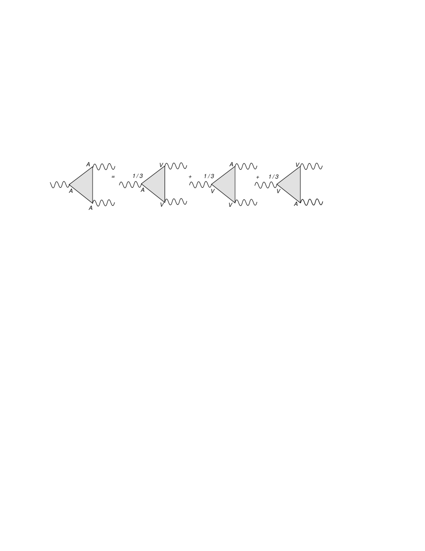
Figure 22: Distribution of the axial anomaly for the ${\bf AAA}$ diagram

The regularization of the $\bf AAA$ vertex, instead, has to respect the complete Bose symmetry of the diagram and this can be achieved with the symmetric expression

$$\Delta_{3}^{\lambda\mu\nu}(k_{1},k_{2})=\frac{1}{3}[\Delta^{\lambda\mu\nu}(k_{1},k_{2})+\Delta^{\mu\nu\lambda}(k_{2},-k)+\Delta^{\nu\lambda\mu}(-k,k_{1})].$$ (129)

It is an easy exercise to show that this symmetric choice is independent from the momentum shift

$$\Delta_{3}^{\lambda\mu\nu}(\beta,k_{1},k_{2})=\Delta_{3}^{\lambda\mu\nu}(k_{1},k_{2})$$ (130)

and that the anomaly is equally distributed among the 3 vertices, $a_{1}=a_{2}=a_{3}=a_{n}/3$, as shown in Fig.  22. We conclude this section with some comments regarding the kind of invariant amplitudes appearing in the definition of $\Delta$ which help to clarify the role of the CS terms in the parameterization of these diagrams in momentum space. For $\overline{\Delta}_{{\lambda}\mu\nu}^{({\bf AVV})}$, expressed using Rosenberg’s parametrization, one obtains

$$\overline{\Delta}_{{\lambda}\mu\nu} = \hat{a}_{1}\epsilon[k_{1},\mu,\nu,\lambda]+\hat{a}_{2}\epsilon[k_{2},\mu,\nu,\lambda]+\hat{a}_{3}\epsilon[k_{1},k_{2},\mu,\lambda]{k_{1}}^{\nu}$$ (131)

$$+\hat{a}_{4}\epsilon[k_{1},k_{2},\mu,\lambda]k_{2}^{\nu}+\hat{a}_{5}\epsilon[k_{1},k_{2},\nu,\lambda]k_{1}^{\mu}+\hat{a}_{6}\epsilon[k_{1},k_{2},\nu,\lambda]k_{2}^{\mu},$$

originally given in [15], with $\lambda$ being the axial-vector vertex. By power-counting, 2 invariant amplitudes are divergent, $a_{1}$ and $a_{2}$, while the $a_{i}$ with $i\geq 3$ are finite.

Instead, for the direct plus the exchanged diagrams we use the expression

$$\Delta_{\underline{\lambda}\mu\nu}+\Delta_{\underline{\lambda}\nu\mu} = (\hat{a}_{1}-\hat{a}_{2})\epsilon[k_{1},\mu,\nu,\lambda]+(a_{2}-a_{1})\epsilon[k_{2},\mu,\nu,\lambda]$$ (132)

$$+(\hat{a}_{3}-\hat{a}_{6})\epsilon[k_{1},k_{2},\mu,\lambda]{k_{1}}^{\nu}+(\hat{a}_{4}-\hat{a}_{5})\epsilon[k_{1},k_{2},\mu,\lambda]k_{2}^{\nu}$$

$$+(\hat{a}_{5}-\hat{a}_{4})\epsilon[k_{1},k_{2},\nu,\lambda]k_{1}^{\mu}+(\hat{a}_{6}-\hat{a}_{3})\epsilon[k_{1},k_{2},\nu,\lambda]k_{2}^{\mu}$$

$$= \underline{a}_{1}\epsilon[k_{1},\mu,\nu,\lambda]+\underline{a}_{2}\epsilon[k_{2},\mu,\nu,\lambda]+\underline{a}_{3}\epsilon[k_{1},k_{2},\mu,\lambda]{k_{1}}^{\nu}$$

$$+\underline{a}_{4}\epsilon[k_{1},k_{2},\mu,\lambda]{k_{2}}^{\nu}+\underline{a}_{5}\epsilon[k_{1},k_{2},\nu,\lambda]k_{1}^{\mu}+\underline{a}_{6}\epsilon[k_{1},k_{2},\nu,\lambda]k_{2}^{\mu}$$

where clearly $\underline{a}_{2}=-\underline{a}_{1},\underline{a}_{3}=-\underline{a}_{6}$ and $\underline{a}_{4}=-\underline{a}_{5}$. The CS contributions are those proportional to the two terms linear in the external momenta. We recall that in Rosenberg, these linear terms are re-expressed in terms of the remaining ones by imposing the vector Ward identities on the V-lines. As already explained, we will instead assume, in our case, that the distribution of the anomaly among the 3 vertices of all the anomalous diagrams of the theory respects the requirement of Bose symmetry, with no additional constraint. A discussion of some technical points concerning the regularization of this and other diagrams both in 4 dimensions and in other schemes, such as Dimensional Regularization (DR) can be found below. For instance, one can find there the proof of the identical vanishing of $\Delta_{\bf VVV}$ worked out in both schemes. In this last case this result is obtained after removing the so called hat-momenta of the t’Hooft-Veltman scheme on the external lines. In this scheme this is possible since one can choose the external momenta to lay on a four-dimensional subspace (see [26] for a discussion of these methods). We remark also that it is also quite useful to be able to switch from momentum space to configuration space with ease, and for this purpose we introduce the Fourier transforms of (19) and (20) in the anomaly equations, obtaining their expressions in configuration space

$$\frac{\partial}{\partial x^{\mu}}T^{\lambda\mu\nu}_{\bf AVV}(x,y,z) = ia_{1}(\beta)\epsilon^{\lambda\nu\alpha\beta}\frac{\partial}{\partial x^{\alpha}}\frac{\partial}{\partial y^{\beta}}\left(\delta^{4}(x-z)\delta^{4}(y-z)\right),$$

$$\frac{\partial}{\partial y^{\nu}}T^{\lambda\mu\nu}_{\bf AVV}(x,y,z) = ia_{2}(\beta)\epsilon^{\lambda\mu\alpha\beta}\frac{\partial}{\partial y^{\alpha}}\frac{\partial}{\partial x^{\beta}}\left(\delta^{4}(x-z)\delta^{4}(y-z)\right),$$

$$\frac{\partial}{\partial z^{\lambda}}T^{\lambda\mu\nu}_{\bf AVV}(x,y,z) = ia_{3}(\beta)\epsilon^{\mu\nu\alpha\beta}\frac{\partial}{\partial x^{\alpha}}\frac{\partial}{\partial y^{\beta}}\left(\delta^{4}(x-z)\delta^{4}(y-z)\right),$$ (133)

with $a_{1},a_{2}$ and $a_{3}$ as in (127), for the $\bf AVV$ case and

$$\frac{\partial}{\partial x^{\mu}}T^{\lambda\mu\nu}_{\bf AAA}(x,y,z) = i\frac{a_{n}}{3}\epsilon^{\lambda\nu\alpha\beta}\frac{\partial}{\partial x^{\alpha}}\frac{\partial}{\partial y^{\beta}}\left(\delta^{4}(x-z)\delta^{4}(y-z)\right),$$

$$\frac{\partial}{\partial y^{\nu}}T^{\lambda\mu\nu}_{\bf AAA}(x,y,z) = i\frac{a_{n}}{3}\epsilon^{\lambda\mu\alpha\beta}\frac{\partial}{\partial y^{\alpha}}\frac{\partial}{\partial x^{\beta}}\left(\delta^{4}(x-z)\delta^{4}(y-z)\right),$$

$$\frac{\partial}{\partial z^{\lambda}}T^{\lambda\mu\nu}_{\bf AAA}(x,y,z) = i\frac{a_{n}}{3}\epsilon^{\mu\nu\alpha\beta}\frac{\partial}{\partial x^{\alpha}}\frac{\partial}{\partial y^{\beta}}\left(\delta^{4}(x-z)\delta^{4}(y-z)\right),$$ (134)

for the $\bf AAA$ case. Notice that in this last case we have distributed the anomaly equally among the three vertices. These relations will be needed when we derive the anomalous variation of the effective action directly in configuration space.

13 Appendix. Chern Simons cancelations

Having isolated the CS contributions, as shown in Fig. 6, the cancelation of the gauge dependence can be obtained combining all these terms so to obtain

$$S_{\xi} = \Delta^{\lambda\mu\nu}(-k_{1},-k_{2})\left[\frac{-i}{k^{2}-\xi_{B}M^{2}_{1}}\frac{k^{\lambda}k^{\lambda^{\prime}}}{M^{2}_{1}}\right]\Delta^{\lambda^{\prime}\mu^{\prime}\nu^{\prime}}(k_{1},k_{2})$$ (135)

$$+ 4\times\left(\frac{4}{M}C_{AA}\right)^{2}\epsilon^{\mu\nu\rho\sigma}k_{1\rho}k_{2\sigma}\left[\frac{i}{k^{2}-\xi_{B}M^{2}_{1}}\right]\epsilon^{\mu^{\prime}\nu^{\prime}\rho^{\prime}\sigma^{\prime}}k_{1\rho^{\prime}}k_{2\sigma^{\prime}}$$

$$+ 4\times(id_{1}\epsilon^{\mu\nu\lambda\sigma}(k_{1}-k_{2})_{\sigma})\left[\frac{-i}{k^{2}-\xi_{B}M^{2}_{1}}\frac{k^{\lambda}k^{\lambda^{\prime}}}{M^{2}_{1}}\right](-id_{1}\epsilon^{\mu^{\prime}\nu^{\prime}\lambda^{\prime}\sigma^{\prime}}(k_{1}-k_{2})_{\sigma^{\prime}})$$

$$+ 2\times\Delta^{\lambda\mu\nu}(-k_{1},-k_{2})\left[\frac{-i}{k^{2}-\xi_{B}M^{2}_{1}}\frac{k^{\lambda}k^{\lambda^{\prime}}}{M^{2}_{1}}\right](-id_{1}\epsilon^{\mu^{\prime}\nu^{\prime}\lambda^{\prime}\sigma^{\prime}}(k_{1}-k_{2})_{\sigma^{\prime}})$$

$$+ 2\times(id_{1}\epsilon^{\mu\nu\lambda\sigma}(k_{1}-k_{2})_{\sigma})\left[\frac{-i}{k^{2}-\xi_{B}M^{2}_{1}}\frac{k^{\lambda}k^{\lambda^{\prime}}}{M^{2}_{1}}\right]\Delta^{\lambda^{\prime}\mu^{\prime}\nu^{\prime}}(k_{1},k_{2}),$$

and using the relevant Ward identities these simply so to obtain

$$S_{\xi} = (-a_{3}(\beta)\epsilon^{\mu\nu\rho\sigma}k_{1\rho}k_{2\sigma})\left[\frac{-i}{k^{2}-\xi_{B}M^{2}_{1}}\frac{1}{M^{2}_{1}}\right](a_{3}(\beta)\epsilon^{\mu^{\prime}\nu^{\prime}\rho^{\prime}\sigma^{\prime}}k_{1\rho^{\prime}}k_{2\sigma^{\prime}})$$ (136)

$$+ 4\times\frac{16}{M^{2}}\left[\left(-\frac{d_{1}}{2}+\frac{i}{2}a_{3}(\beta)\frac{1}{4}\right)^{2}\frac{M^{2}}{M^{2}_{1}}\right]\epsilon^{\mu\nu\rho\sigma}k_{1\rho}k_{2\sigma}\left[\frac{i}{k^{2}-\xi_{B}M^{2}_{1}}\right]\epsilon^{\mu^{\prime}\nu^{\prime}\rho^{\prime}\sigma^{\prime}}k_{1\rho^{\prime}}k_{2\sigma^{\prime}}$$

$$+ 4\times d^{2}_{1}\left[\frac{-i}{k^{2}-\xi_{B}M^{2}_{1}}\frac{1}{M^{2}_{1}}\right]4\epsilon^{\mu\nu\rho\sigma}k_{1\rho}k_{2\sigma}\epsilon^{\mu^{\prime}\nu^{\prime}\rho^{\prime}\sigma^{\prime}}k_{1\rho^{\prime}}k_{2\sigma^{\prime}}$$

$$+ 2\times(-a_{3}(\beta)\epsilon^{\mu\nu\rho\sigma}k_{1\rho}k_{2\sigma})\left[\frac{-i}{k^{2}-\xi_{B}M^{2}_{1}}\frac{1}{M^{2}_{1}}\right](+id_{1}2\epsilon^{\mu^{\prime}\nu^{\prime}\lambda^{\prime}\sigma^{\prime}}k^{\lambda^{\prime}}_{1}k^{\sigma^{\prime}}_{2})$$

$$+ 2\times(-id_{1}2\epsilon^{\mu\nu\lambda\sigma}k^{\lambda}_{1}k^{\sigma}_{2})\left[\frac{-i}{k^{2}-\xi_{B}M^{2}_{1}}\frac{1}{M^{2}_{1}}\right](a_{3}(\beta)\epsilon^{\mu^{\prime}\nu^{\prime}\rho^{\prime}\sigma^{\prime}}k_{1\rho^{\prime}}k_{2\sigma^{\prime}})=0.$$

Having shown the cancelation of the gauge-dependent terms, the gauge independent contribution becomes

$$S_{0} = \Delta^{\lambda\mu\nu}(-k_{1},-k_{2})\left[\frac{-i}{k^{2}-M^{2}_{1}}\left(g^{\lambda\lambda^{\prime}}-\frac{k^{\lambda}k^{\lambda^{\prime}}}{M^{2}_{1}}\right)\right]\Delta^{\lambda^{\prime}\mu^{\prime}\nu^{\prime}}(k_{1},k_{2})$$ (137)

$$+ 4\times(id_{1}\epsilon^{\,\mu\nu\lambda\sigma}(k_{1}-k_{2})_{\sigma})\left[\frac{-i}{k^{2}-M^{2}_{1}}\left(g^{\lambda\lambda^{\prime}}-\frac{k^{\lambda}k^{\lambda^{\prime}}}{M^{2}_{1}}\right)\right](-id_{1}\epsilon^{\,\mu^{\prime}\nu^{\prime}\lambda^{\prime}\sigma^{\prime}}(k_{1}-k_{2})_{\sigma^{\prime}})$$

$$+ 2\times\Delta^{\lambda\mu\nu}(-k_{1},-k_{2})\left[\frac{-i}{k^{2}-M^{2}_{1}}\left(g^{\lambda\lambda^{\prime}}-\frac{k^{\lambda}k^{\lambda^{\prime}}}{M^{2}_{1}}\right)\right](-id_{1}\epsilon^{\,\mu^{\prime}\nu^{\prime}\lambda^{\prime}\sigma^{\prime}}(k_{1}-k_{2})_{\sigma^{\prime}})$$

$$+ 2\times(id_{1}\epsilon^{\,\mu\nu\lambda\sigma}(k_{1}-k_{2})_{\sigma})\left[\frac{-i}{k^{2}-M^{2}_{1}}\left(g^{\lambda\lambda^{\prime}}-\frac{k^{\lambda}k^{\lambda^{\prime}}}{M^{2}_{1}}\right)\right]\Delta^{\lambda^{\prime}\mu^{\prime}\nu^{\prime}}(k_{1},k_{2}).$$

At this point we need to express the triangle diagrams in terms of their shifting parameter $\beta$ using the shift-relations

$$\Delta^{\lambda\mu\nu}(\beta,k_{1},k_{2})=\Delta^{\lambda\mu\nu}(k_{1},k_{2})-\frac{i}{4\pi^{2}}\beta\epsilon^{\lambda\mu\nu\sigma}(k_{1}-k_{2})_{\sigma},$$ (138)

$$\Delta^{\lambda\mu\nu}(\beta,-k_{1},-k_{2})=\Delta^{\lambda\mu\nu}(-k_{1},-k_{2})+\frac{i}{4\pi^{2}}\beta\epsilon^{\lambda\mu\nu\sigma}(k_{1}-k_{2})_{\sigma},$$ (139)

and with the substitution $d_{1}=-ia_{1}(\beta)/2$ we obtain

$$S_{0} = \left(\Delta^{\lambda\mu\nu}(-k_{1},-k_{2})+\frac{i}{4\pi^{2}}\beta\epsilon^{\,\lambda\mu\nu\sigma}(k_{1}-k_{2})_{\sigma}\right)P^{\lambda\lambda^{\prime}}_{0}\left(\Delta^{\lambda^{\prime}\mu^{\prime}\nu^{\prime}}(k_{1},k_{2})-\frac{i}{4\pi^{2}}\beta\epsilon^{\,\lambda^{\prime}\mu^{\prime}\nu^{\prime}\sigma^{\prime}}(k_{1}-k_{2})_{\sigma^{\prime}}\right)$$ (140)

$$+ 4\times\left(\frac{1}{2}a_{1}(\beta)\epsilon^{\,\mu\nu\lambda\sigma}(k_{1}-k_{2})_{\sigma}\right)P^{\lambda\lambda^{\prime}}_{0}\left(-\frac{1}{2}a_{1}(\beta)\epsilon^{\,\mu^{\prime}\nu^{\prime}\lambda^{\prime}\sigma^{\prime}}(k_{1}-k_{2})_{\sigma^{\prime}}\right)$$

$$+ 2\times\left(\Delta^{\lambda\mu\nu}(-k_{1},-k_{2})+\frac{i}{4\pi^{2}}\beta\epsilon^{\,\lambda\mu\nu\sigma}(k_{1}-k_{2})_{\sigma}\right)P^{\lambda\lambda^{\prime}}_{0}\left(-\frac{1}{2}a_{1}(\beta)\epsilon^{\,\mu^{\prime}\nu^{\prime}\lambda^{\prime}\sigma^{\prime}}(k_{1}-k_{2})_{\sigma^{\prime}}\right)$$

$$+ 2\times\left(\frac{1}{2}a_{1}(\beta)\epsilon^{\,\mu\nu\lambda\sigma}(k_{1}-k_{2})_{\sigma}\right)P^{\lambda\lambda^{\prime}}_{0}\left(\Delta^{\lambda^{\prime}\mu^{\prime}\nu^{\prime}}(k_{1},k_{2})-\frac{i}{4\pi^{2}}\beta\epsilon^{\,\lambda^{\prime}\mu^{\prime}\nu^{\prime}\sigma^{\prime}}(k_{1}-k_{2})_{\sigma^{\prime}}\right).$$

Introducing the explicit expression for $a_{1}(\beta)$, it is an easy exercise to show the equivalence between $S_{0}$ and diagram A of Fig. 6, with a choice of the shifting parameter that corresponds to the CVC condition ($\beta=-1/2$)

$$S_{0}\equiv\left(\Delta^{\lambda\mu\nu}(-k_{1},-k_{2})-\frac{i}{8\pi^{2}}\epsilon^{\,\lambda\mu\nu\sigma}(k_{1}-k_{2})_{\sigma}\right)P^{\lambda\lambda^{\prime}}_{0}\left(\Delta^{\lambda^{\prime}\mu^{\prime}\nu^{\prime}}(k_{1},k_{2})+\frac{i}{8\pi^{2}}\beta\epsilon^{\,\lambda^{\prime}\mu^{\prime}\nu^{\prime}\sigma^{\prime}}(k_{1}-k_{2})_{\sigma^{\prime}}\right).$$

13.1 Cancelation of gauge dependences in the broken Higgs phase

In this case we have (see Fig. 7)

$$S_{\xi} = A_{\xi}+B_{\xi}+C_{\xi}+D_{\xi}+E_{\xi}+F_{\xi}+G_{\xi}+H_{\xi}$$

$$= \Delta^{\lambda\mu\nu}(-k_{1},-k_{2})\left[\frac{-i}{k^{2}-\xi_{B}M^{2}_{B}}\frac{k^{\lambda}k^{\lambda^{\prime}}}{M^{2}_{B}}\right]\Delta^{\lambda^{\prime}\mu^{\prime}\nu^{\prime}}(k_{1},k_{2})$$

$$+ 4\times\left(\frac{4}{M}\alpha_{2}C_{AA}\right)^{2}\epsilon^{\mu\nu\rho\sigma}k_{1\rho}k_{2\sigma}\left[\frac{i}{k^{2}-\xi_{B}M^{2}_{B}}\right]\epsilon^{\mu^{\prime}\nu^{\prime}\rho^{\prime}\sigma^{\prime}}k_{1\rho^{\prime}}k_{2\sigma^{\prime}}$$

$$+ 4\times(id_{1}\epsilon^{\mu\nu\lambda\sigma}(k_{1}-k_{2})_{\sigma})\left[\frac{-i}{k^{2}-\xi_{B}M^{2}_{B}}\frac{k^{\lambda}k^{\lambda^{\prime}}}{M^{2}_{B}}\right](-id_{1}\epsilon^{\mu^{\prime}\nu^{\prime}\lambda^{\prime}\sigma^{\prime}}(k_{1}-k_{2})_{\sigma^{\prime}})$$

$$+ 2\times\Delta^{\lambda\mu\nu}(-k_{1},-k_{2})\left[\frac{-i}{k^{2}-\xi_{B}M^{2}_{B}}\frac{k^{\lambda}k^{\lambda^{\prime}}}{M^{2}_{B}}\right](-id_{1}\epsilon^{\mu^{\prime}\nu^{\prime}\lambda^{\prime}\sigma^{\prime}}(k_{1}-k_{2})_{\sigma^{\prime}})$$

$$+ 2\times(id_{1}\epsilon^{\mu\nu\lambda\sigma}(k_{1}-k_{2})_{\sigma})\left[\frac{-i}{k^{2}-\xi_{B}M^{2}_{B}}\frac{k^{\lambda}k^{\lambda^{\prime}}}{M^{2}_{B}}\right]\Delta^{\lambda^{\prime}\mu^{\prime}\nu^{\prime}}(k_{1},k_{2})$$

$$+ 2\times\Delta^{\mu\nu}(-k_{1},-k_{2})\left(2i\frac{m_{f}}{M_{B}}\right)\left[\frac{i}{k^{2}-\xi_{B}M^{2}_{B}}\right]\left(\frac{4}{M}\alpha_{2}C_{AA}\epsilon^{\mu^{\prime}\nu^{\prime}\rho^{\prime}\sigma^{\prime}}k_{1\rho^{\prime}}k_{2\sigma^{\prime}}\right)$$

$$+ \Delta^{\mu\nu}(-k_{1},-k_{2})\left(2i\frac{m_{f}}{M_{B}}\right)\left[\frac{i}{k^{2}-\xi_{B}M^{2}_{B}}\right]\left(2i\frac{m_{f}}{M_{B}}\right)\Delta^{\mu^{\prime}\nu^{\prime}}(k_{1},k_{2})$$

$$+ 2\times\left(\frac{4}{M}\alpha_{2}C_{AA}\epsilon^{\mu\nu\rho\sigma}k_{1\rho}k_{2\sigma}\right)\left[\frac{i}{k^{2}-\xi_{B}M^{2}_{B}}\right]\left(2i\frac{m_{f}}{M_{B}}\right)\Delta^{\mu\nu}(k_{1},k_{2})$$

The vanishing of this expression cna be checked as in the previous case, using the massive version of the anomalous Ward identities in the triangular graphs involving $\Delta$.

13.2 Cancelations in the A-B Model: BB $\rightarrow$ BB mediated by a B gauge boson

Let’s now discuss the exchange of a B gauge boson in the s-channel before spontaneous symmetry breaking. The relevant diagrams are shown in Fig. 23. We remark, obviously, that each diagram has to be inserted with the correct multiplicity factor in order to obtain the cancelation of the unphysical poles.

Figure 23: Relevant diagrams for the unitarity check before symmetry breaking.

In this case, from Bose-symmetry, the anomaly is equally distributed among the 3 vertices, $a_{1}=a_{2}=a_{3}=a_{n}/3$, as we have discussed above. We recall that from the variations $\delta_{B}\mathcal{L}_{an}$ and $\delta_{B}\mathcal{L}_{b}$ the relevant terms are

$$\frac{1}{3!}\delta_{B}\langle T_{BBB}^{\lambda\mu\nu}B^{\lambda}(z)B^{\mu}(x)B^{\nu}(y)\rangle = \,\frac{ig^{\,3}_{B}}{3!}\,a_{n}\langle\theta_{B}\,\,\frac{F^{B}\wedge F^{B}}{4}\rangle$$

$$\delta_{B}\langle\frac{C_{BB}}{M}\,bF^{B}\wedge F^{B}\rangle = -\,C_{BB}\frac{M_{1}}{M}\langle\theta_{B}F^{B}\wedge F^{B}\rangle\;\;\;\mbox{from}\;\;\;\delta_{B}b=-M_{1}\theta_{B},$$

so that from the condition of anomaly cancelation we obtain

$$-C_{BB}\frac{M_{1}}{M}+\frac{ig^{\,3}_{B}}{3!}\,\frac{1}{4}\,a_{n}=0\,\,\Longleftrightarrow\,\,C_{BB}=\,\frac{ig^{\,3}_{B}}{3!}\,\frac{1}{4}\,a_{n}\frac{M}{M_{1}},$$ (144)

which fixes the appropriate value of the coefficient of the WZ term. One can easily show the correspondence between a Green-Schwarz term $\frac{C_{BB}}{M}\,b\,F^{B}\wedge F^{B}$ and a vertex $4\frac{C_{BB}}{M}\,\varepsilon^{\mu\nu\rho\sigma}k_{1}^{\rho}k_{2}^{\sigma}$ in momentum representation, a derivation of which can be found in an appendix.

Taking into account only the gauge-dependent parts of the two diagrams, we have that the diagram with the exchange of the gauge boson B can be written as

$$\mathcal{A}_{\xi}=\Delta^{\lambda\,\mu\,\nu}(-k_{1},-k_{2})\left[\frac{-\,i}{k^{2}-\xi_{B}M_{1}^{2}}\left(\frac{k^{\lambda}\,k^{\lambda^{\prime}}}{M_{1}^{2}}\right)\right]\Delta^{\lambda^{\prime}\,\mu^{\prime}\,\nu^{\prime}}(k_{1},k_{2})$$ (145)

and the diagram with the exchange of the axion b is

$$\mathcal{B}_{\xi}=4\times\left(\frac{4}{M}C_{BB}\right)^{2}\varepsilon^{\mu\nu\rho\sigma}k_{1}^{\rho}k_{2}^{\sigma}\left(\frac{i}{k^{2}-\xi_{B}M_{1}^{2}}\right)\varepsilon^{\mu^{\prime}\nu^{\prime}\rho^{\prime}\sigma^{\prime}}k_{1}^{\rho^{\prime}}k_{2}^{\sigma^{\prime}}.$$ (146)

Using the anomaly equations for the AAA vertex we can evaluate the first diagram

$$\mathcal{A}_{\xi} = \frac{-\,i}{k^{2}-\xi_{B}M_{1}^{2}}\frac{1}{M_{1}^{2}}\left(k^{\lambda}\Delta^{\lambda\mu\nu}\right)\left(k^{\lambda^{\prime}}\Delta^{\lambda^{\prime}\mu^{\prime}\nu^{\prime}}\right)$$ (147)

$$= \frac{-\,i}{k^{2}-\xi_{B}M_{1}^{2}}\frac{1}{M_{1}^{2}}\left(-(\,g_{B})^{3}\,\frac{a_{n}}{3}\varepsilon^{\mu\nu\alpha\beta}k_{1}^{\alpha}k_{2}^{\beta}\right)\left((\,g_{B})^{3}\,\frac{a_{n}}{3}\varepsilon^{\mu^{\prime}\nu^{\prime}\alpha^{\prime}\beta^{\prime}}k_{1}^{\alpha^{\prime}}k_{2}^{\beta^{\prime}}\right)$$

$$= \frac{\,i}{k^{2}-\xi_{B}M_{1}^{2}}\frac{1}{M_{1}^{2}}\left(\frac{a_{n}}{3}\,g^{\,3}_{B}\right)^{2}\,\varepsilon^{\mu\nu\alpha\beta}\,\varepsilon^{\mu^{\prime}\nu^{\prime}\alpha^{\prime}\beta^{\prime}}\,k_{1}^{\alpha}k_{2}^{\beta}\,k_{1}^{\alpha^{\prime}}k_{2}^{\beta^{\prime}},$$

while the axion exchange diagram gives

$$\mathcal{B}_{\xi} = 4\times\left(\frac{4C_{BB}}{M}\right)^{2}\left(\frac{i}{k^{2}-\xi_{B}M_{1}^{2}}\right)\varepsilon^{\mu\nu\alpha\beta}\,\varepsilon^{\mu^{\prime}\nu^{\prime}\alpha^{\prime}\beta^{\prime}}\,k_{1}^{\alpha}k_{2}^{\beta}\,k_{1}^{\alpha^{\prime}}k_{2}^{\beta^{\prime}}$$ (148)

$$= \frac{64\,\,{C^{\,2}_{BB}}}{M^{2}}\frac{i}{k^{2}-\xi_{B}M_{1}^{2}}\,\varepsilon^{\mu\nu\alpha\beta}\,\varepsilon^{\mu^{\prime}\nu^{\prime}\alpha^{\prime}\beta^{\prime}}\,k_{1}^{\alpha}k_{2}^{\beta}\,k_{1}^{\alpha^{\prime}}k_{2}^{\beta^{\prime}}.$$

Adding the contributions from the two diagrams we obtain

$$\mathcal{A}_{\xi}+\mathcal{B}_{\xi}=0\,\,\,\Longleftrightarrow\,\,\,\frac{1}{M_{1}^{2}}\left(\frac{a_{n}}{3}\,g^{\,3}_{B}\right)^{2}+\frac{64\,\,{C^{\,2}_{BB}}}{M^{2}}=0,$$ (149)

in fact substituting the proper value for the coefficient $C_{BB}$ we obtain an identity

$$\frac{1}{M_{1}^{2}}\frac{a_{n}^{2}}{9}\,g^{\,6}_{B}+\frac{64}{M^{2}}\left[\,\frac{ig^{\,3}_{B}}{3!}\,\frac{1}{4}\,a_{n}\frac{M}{M_{1}}\right]^{2}=\frac{1}{M_{1}^{2}}\frac{a_{n}^{2}}{9}g^{\,6}_{B}-\frac{64}{M_{1}^{2}}\frac{1}{64}\frac{a_{n}^{2}}{9}g^{\,6}_{B}=0.$$ (150)

This pattern of cancelations holds for a massless fermion ($m_{f}=0$).

13.3 Gauge cancelations in the self-energy diagrams

In this case, following Fig. 9, we isolate the following gauge-dependent amplitudes

$${\mathcal{A}}_{\xi 0} = \,\Delta^{\lambda\mu\nu}(-k_{1},-k_{2})\left[\frac{-i}{k^{2}-\xi_{B}M^{2}_{B}}\left(\frac{k^{\lambda}k^{\lambda^{\prime}}}{M^{2}_{B}}\right)\right]\Delta^{\lambda^{\prime}\mu^{\prime}\nu^{\prime}}(k_{1},k_{2})\,P^{\nu\nu^{\prime}}_{o},$$

$${\mathcal{B}}_{\xi 0} = 4\times\left(\frac{4}{M}\alpha_{2}C_{AA}\right)^{2}\epsilon^{\,\mu\nu\rho\sigma}k_{1\rho}k_{2\sigma}\frac{i}{k^{2}-\xi_{B}M^{2}_{B}}\epsilon^{\,\mu^{\prime}\nu^{\prime}\rho^{\prime}\sigma^{\prime}}k_{1\rho^{\prime}}k_{2\sigma^{\prime}}\,P^{\nu\nu^{\prime}}_{o},$$

$${\mathcal{C}}_{\xi 0} = \Delta^{\mu\nu}(-k_{1},-k_{2})\left(2i\frac{m_{f}}{M_{B}}\right)\frac{i}{k^{2}-\xi_{B}M^{2}_{B}}\left(2i\frac{m_{f}}{M_{B}}\right)\Delta^{\mu^{\prime}\nu^{\prime}}(k_{1},k_{2})P^{\nu\nu^{\prime}}_{o},$$

$${\mathcal{D}}_{\xi 0} = 2\times\left(\frac{4}{M}\alpha_{2}C_{AA}\epsilon^{\,\mu\nu\rho\sigma}k_{1\rho}k_{2\sigma}\right)\frac{i}{k^{2}-\xi_{B}M^{2}_{B}}\left(2i\frac{m_{f}}{M_{B}}\right)\Delta^{\mu^{\prime}\nu^{\prime}}(k_{1},k_{2})P^{\nu\nu^{\prime}}_{o},$$

$${\mathcal{E}}_{\xi 0} = 2\times\Delta^{\mu\nu}(-k_{1},-k_{2})\left(2i\frac{m_{f}}{M_{B}}\right)\frac{i}{k^{2}-\xi_{B}M^{2}_{B}}\left(\frac{4}{M}\alpha_{2}C_{AA}\epsilon^{\,\mu^{\prime}\nu^{\prime}\rho^{\prime}\sigma^{\prime}}k_{1\rho^{\prime}}k_{2\sigma^{\prime}}\right)P^{\nu\nu^{\prime}}_{o},$$

so that using the anomaly equations for the triangles

$$k^{\lambda^{\prime}}\Delta^{\lambda^{\prime}\mu^{\prime}\nu^{\prime}}(k_{1},k_{2}) = a_{3}(\beta)\epsilon^{\,\mu^{\prime}\nu^{\prime}\rho^{\prime}\sigma^{\prime}}k_{1\rho^{\prime}}k_{2\sigma^{\prime}}+2m_{f}\Delta^{\mu^{\prime}\nu^{\prime}},$$

$$k^{\lambda}\Delta^{\lambda\mu\nu}(-k_{1},-k_{2}) = -a_{3}(\beta)\epsilon^{\,\mu\nu\rho\sigma}k_{1\rho}k_{2\sigma}-2m_{f}\Delta^{\mu\nu},$$

and substituting the appropriate value for the WZ-coefficient, with the rotation coefficient of the axion $b$ to the goldstone boson given by $\alpha_{2}=M_{1}/M_{B}$, one obtains quite straightforwardly that the condition of gauge independence is satisfied

$${\mathcal{A}}_{\xi 0}+{\mathcal{B}}_{\xi 0}+{\mathcal{C}}_{\xi 0}+{\mathcal{D}}_{\xi 0}+{\mathcal{E}}_{\xi 0}=0.$$ (152)

14 Ward identities on the tetragon

As we have seen in the previous sections, the shift dependence from the anomaly on each vertex, parameterized by $\beta,\beta_{1},\beta_{2}$, drops in the actual computation of the unitarity conditions on the s-channel amplitudes, which clearly signals the irrelevance of these shifts in the actual computation, as far as the Bose symmetry of the corresponding amplitudes that assign the anomaly on each vertex consistently, are respected. It is well known that all the contribution of the anomaly in correlators with more external legs is taken care of by the correct anomaly cancelation in 3-point function. It is instructive to illustrate, for generic shifts, chosen so to respect the symmetries of the higher point functions, how a similar patterns holds. This takes place since anomalous Ward identities for higher order correlators are expressed in terms of standard triangle anomalies. This analysis and a similar analysis of other diagrams of this type, which we have included in an appendix, is useful for the investigation of some rare Z decays (such as Z to 3 photons) which takes place with an on-shell Z boson.

Then let’s consider the tetragon diagram BAAA shown in fig.(24), where B, being characterized by an axial-vector coupling, generates an anomaly in the related Ward identity.

Figure 24: The tetragon contribution.

We have the fermionic trace

$$\Delta^{\lambda\mu\nu\rho}(k_{1},k_{2},k_{3})=\overline{\Delta}^{\lambda\mu\nu\rho}(k_{1},k_{2},k_{3})+\mbox{perm.}$$ (153)

where perm. means permutations of $\{(k_{1},\mu),(k_{2},\nu),(k_{3},\rho)\}$. One contribution to the axial Ward identity comes for instance from

$$k^{\lambda}Tr\left[\gamma^{\lambda}\gamma^{5}\frac{1}{p\hskip-6.0pt/\hskip 6.0pt-k\hskip-6.0pt/\hskip 6.0pt}\gamma^{\rho}\frac{1}{p\hskip-6.0pt/\hskip 6.0pt-k\kern-4.30554pt\hbox{/}_{1}-k\kern-4.30554pt\hbox{/}_{2}}\gamma^{\nu}\frac{1}{p\hskip-6.0pt/\hskip 6.0pt-k\kern-4.30554pt\hbox{/}_{1}}\gamma^{\mu}\frac{1}{p\hskip-6.0pt/\hskip 6.0pt}\right]$$ (154)

$$= Tr\left[k\hskip-6.0pt/\hskip 6.0pt\gamma^{5}\frac{1}{p\hskip-6.0pt/\hskip 6.0pt-k\hskip-6.0pt/\hskip 6.0pt}\gamma^{\rho}\frac{1}{p\hskip-6.0pt/\hskip 6.0pt-k\kern-4.30554pt\hbox{/}_{1}-k\kern-4.30554pt\hbox{/}_{2}}\gamma^{\nu}\frac{1}{p\hskip-6.0pt/\hskip 6.0pt-k\kern-4.30554pt\hbox{/}_{1}}\gamma^{\mu}\frac{1}{p\hskip-6.0pt/\hskip 6.0pt}\right]$$

$$= -Tr\left[\gamma^{5}\frac{1}{p\hskip-6.0pt/\hskip 6.0pt}\gamma^{\rho}\frac{1}{p\hskip-6.0pt/\hskip 6.0pt-k\kern-4.30554pt\hbox{/}_{1}-k\kern-4.30554pt\hbox{/}_{2}}\gamma^{\nu}\frac{1}{p\hskip-6.0pt/\hskip 6.0pt-k\kern-4.30554pt\hbox{/}_{1}}\gamma^{\mu}\right]$$

$$+Tr\left[\gamma^{5}\frac{1}{p\hskip-6.0pt/\hskip 6.0pt-k\hskip-6.0pt/\hskip 6.0pt}\gamma^{\rho}\frac{1}{p\hskip-6.0pt/\hskip 6.0pt-k\kern-4.30554pt\hbox{/}_{1}-k\kern-4.30554pt\hbox{/}_{2}}\gamma^{\nu}\frac{1}{p\hskip-6.0pt/\hskip 6.0pt-k\kern-4.30554pt\hbox{/}_{1}}\gamma^{\mu}\right],$$

which has been rearranged in terms of triangle anomalies using

$$\frac{1}{p\hskip-6.0pt/\hskip 6.0pt}k\hskip-6.0pt/\hskip 6.0pt\gamma^{5}\frac{1}{p\hskip-6.0pt/\hskip 6.0pt-k\hskip-6.0pt/\hskip 6.0pt}=\gamma^{5}\frac{1}{p\hskip-6.0pt/\hskip 6.0pt-k\hskip-6.0pt/\hskip 6.0pt}-\gamma^{5}\frac{1}{p\hskip-6.0pt/\hskip 6.0pt}.$$ (155)

Relation (154) is diagrammatically shown in Fig. 25.

Figure 25: Distribution of the moments in the external lines in a Ward identity.

Explicitly these diagrammatic equations become

$$k^{\lambda}\overline{\Delta}^{\lambda\mu\nu\rho} = -\overline{\Delta}^{\rho\mu\nu}(k_{1},k_{2})+\overline{\Delta}^{\mu\nu\rho}(\beta_{1},k_{2},k_{3}),$$

$$k^{\lambda}\overline{\Delta}^{\lambda\mu\rho\nu} = -\overline{\Delta}^{\nu\mu\rho}(k_{1},k_{3})+\overline{\Delta}^{\mu\rho\nu}(\beta_{2},k_{3},k_{2}),$$

$$k^{\lambda}\overline{\Delta}^{\lambda\nu\rho\mu} = -\overline{\Delta}^{\mu\nu\rho}(k_{2},k_{3})+\overline{\Delta}^{\nu\rho\mu}(\beta_{3},k_{3},k_{1}),$$

$$k^{\lambda}\overline{\Delta}^{\lambda\nu\mu\rho} = -\overline{\Delta}^{\rho\nu\mu}(k_{2},k_{1})+\overline{\Delta}^{\nu\mu\rho}(\beta_{4},k_{1},k_{3}),$$

$$k^{\lambda}\overline{\Delta}^{\lambda\rho\mu\nu} = -\overline{\Delta}^{\nu\rho\mu}(k_{3},k_{1})+\overline{\Delta}^{\rho\mu\nu}(\beta_{5},k_{1},k_{2}),$$

$$k^{\lambda}\overline{\Delta}^{\lambda\rho\nu\mu} = -\overline{\Delta}^{\mu\rho\nu}(k_{3},k_{2})+\overline{\Delta}^{\rho\nu\mu}(\beta_{6},k_{2},k_{1}),$$

where the usual (direct) triangle diagram is given for instance by

$$\overline{\Delta}^{\mu\nu\rho}=\int\frac{d^{4}p}{(2\pi)^{4}}Tr\left[\gamma^{\mu}\gamma^{5}\frac{1}{p\hskip-6.0pt/\hskip 6.0pt-k\hskip-6.0pt/\hskip 6.0pt}\gamma^{\rho}\frac{1}{p\hskip-6.0pt/\hskip 6.0pt-k\kern-4.30554pt\hbox{/}_{1}-k\kern-4.30554pt\hbox{/}_{2}}\gamma^{\nu}\frac{1}{p\hskip-6.0pt/\hskip 6.0pt-k\kern-4.30554pt\hbox{/}_{1}}\right].$$ (157)

Adding all the contributions we have

$$k^{\lambda}\Delta^{\lambda\mu\nu\rho}(k_{1},k_{2},k_{3}) = -\left[\Delta^{\rho\mu\nu}(k_{1},k_{2})+\Delta^{\nu\mu\rho}(k_{1},k_{3})+\Delta^{\mu\nu\rho}(k_{2},k_{3})\right]$$

$$+\left[\Delta^{\rho\mu\nu}(\beta_{5},\beta_{6},k_{1},k_{2})+\Delta^{\nu\mu\rho}(\beta_{3},\beta_{4},k_{1},k_{3})+\Delta^{\mu\nu\rho}(\beta_{1},\beta_{2},k_{2},k_{3})\right].$$

At this point, to show the validity of the Ward identity independently of the chosen value of the CS shifts, we recall that under some shifts

$$\Delta^{\mu\nu\rho}(\beta_{1},\beta_{2},k_{2},k_{3}) = \Delta^{\mu\nu\rho}(k_{2},k_{3})-\frac{i(\beta_{1}+\beta_{2})}{4\pi^{2}}\varepsilon^{\mu\nu\rho\sigma}(k_{2}^{\sigma}-k_{3}^{\sigma})$$

$$\Delta^{\nu\mu\rho}(\beta_{3},\beta_{4},k_{2},k_{3}) = \Delta^{\nu\mu\rho}(k_{1},k_{3})-\frac{i(\beta_{3}+\beta_{4})}{4\pi^{2}}\varepsilon^{\nu\mu\rho\sigma}(k_{1}^{\sigma}-k_{3}^{\sigma})$$

$$\Delta^{\rho\mu\nu}(\beta_{5},\beta_{6},k_{1},k_{2}) = \Delta^{\rho\mu\nu}(k_{1},k_{2})-\frac{i(\beta_{5}+\beta_{6})}{4\pi^{2}}\varepsilon^{\rho\mu\nu\sigma}(k_{1}^{\sigma}-k_{2}^{\sigma}),$$

and redefining the shifts by setting

$$\beta_{5}+\beta_{6}=\overline{\beta}_{1}\qquad\beta_{1}+\beta_{2}=\overline{\beta}_{3}\qquad\beta_{3}+\beta_{4}=\overline{\beta}_{2}$$ (160)

we obtain

$$k^{\lambda}\Delta^{\lambda\mu\nu\rho}(k_{1},k_{2},k_{3}) = -\frac{i\overline{\beta}_{1}}{4\pi^{2}}\varepsilon^{\rho\mu\nu\sigma}(k_{1}^{\sigma}-k_{2}^{\sigma})-\frac{i\overline{\beta}_{2}}{4\pi^{2}}\varepsilon^{\nu\mu\rho\sigma}(k_{1}^{\sigma}-k_{3}^{\sigma})$$ (161)

$$-\frac{i\overline{\beta}_{3}}{4\pi^{2}}\varepsilon^{\mu\nu\rho\sigma}(k_{2}^{\sigma}-k_{3}^{\sigma}).$$

Finally, using the Bose symmetry on the r.h.s. (indices $\mu,\nu,\rho$) of the original diagram we obtain

$$\overline{\beta}_{1}=\overline{\beta}_{2}=\overline{\beta}_{3},$$ (162)

which is the correct Ward identity: $k^{\lambda}\Delta^{\lambda\mu\nu\rho}=0$.

Figure 26: The tetragon diagram in non abelian case.

We have shown that the correct choice of the CS shifts in tetragon diagrams, fixed by the requirements of Bose symmetries of the corresponding amplitude and of the underlying 3-point functions, gives the correct Ward identities for these correlators. This is not unexpected, since the anomaly appears only at the level of 3-point functions, but shows how one can work in full generality with these amplitudes and determine their correct structure. It is also interesting to underline the modifications that take place once this study is extended to the non-abelian case. In this case (shown in Fig. 26) one obtains the same result already shown for the axial abelian Ward identity, but modified by color factors. We obtain

$$Tr(\{T^{a},T^{b}\}T^{c})\,[-\Delta^{\rho\mu\nu}+\Delta^{\rho\mu\nu}(\beta)]+Tr(\{T^{c},T^{b}\}T^{a})\,[-\Delta^{\mu\nu\rho}+\Delta^{\mu\nu\rho}(\beta)]$$ (163)

$$+Tr(\{T^{a},T^{c}\}T^{b})\,[-\Delta^{\nu\mu\rho}+\Delta^{\nu\mu\rho}(\beta)]$$

$$= d^{abc}\,[-\Delta^{\rho\mu\nu}+\Delta^{\rho\mu\nu}(\beta)]+d^{cba}\,[-\Delta^{\mu\nu\rho}+\Delta^{\mu\nu\rho}(\beta)]$$

$$+d^{acb}\,[-\Delta^{\nu\mu\rho}+\Delta^{\nu\mu\rho}(\beta)],$$

and we have used the definition of the symmetric d-tensor

$$d^{abc}=Tr(\left\{T^{a},T^{b}\right\}T^{c}).$$ (164)

Simple manipulations give a result which is proportional to the result of the abelian case

$$d^{abc}([-\Delta^{\rho\mu\nu}+\Delta^{\rho\mu\nu}(\beta)]+[-\Delta^{\mu\nu\rho}+\Delta^{\mu\nu\rho}(\beta)]+[-\Delta^{\nu\mu\rho}+\Delta^{\nu\mu\rho}(\beta)]).$$ (165)

The vanishing of the shift-dependence is related to the Bose symmetry under exchange of the indices

$$\{(a,\mu,k_{1}),(b,\nu,k_{2}),(c,\rho,k_{3})\}.$$

This result is clearly expected, since the gauge current of B is abelian and behaves as a gauge-singlet current under the gauge interaction of $A$, the latter having been promoted to a non-abelian current.

15 Appendix. DR-HVBM

In this appendix we fill out some of the details the computation of the direct plus exchanged diagrams in Dimensional Regularization using the HVBM scheme for a partially anticommuting $\gamma_{5}$ [35]. There are various results presented in the previous literature on the computation of these diagrams, most of them using a momentum shift without actually enforcing a regularization, shift that brings the anomaly contribution to the axial-vector vertex of the triangle diagram, keeping the vector Ward identities satisfied, which takes to Rosenberg’s parameterization (185). We fill this gap by showing how the regularization works using an arbitrary tensor structure $T^{\lambda\mu\nu}$ rather than scalar amplitudes. We also keep the mass of the fermion arbitrary, so to obtain a general result concerning the mass dependence of the corrections to the anomaly contributions. We remind that momentum shift are allowed in DR-HVBM, once the integration measure is extended from 4 to $n=4-\epsilon$ dimensions and the Feynman parametrization can be used to reduce the integrals into symmetric forms. Symmetric integration can then be used exactly as in the standard DR case, but with some attention on how to treat the Lorenz indices in the two subspaces of dimensions 4 and $n-4$, introduced by the regularization. These points are illustrated below.

In the following we will use the notation $I_{xy}$ to denote the parametric integration after performing the loop integral

$$I_{xy}\left[...\right]\equiv 2\int_{0}^{1}\int_{0}^{1-x}dy\left[...\right].$$ (166)

There are various ways to implement $\gamma_{5}$ in D-dimensions, but the prescription that works best and is not so difficult to implement is the t’Hooft-Veltman-Breitenlohner-Maison (simply denoted as HVBM) prescription. In the HVBM prescription $\gamma_{5}$ is only partially anticommuting. The gamma algebra in this case is split into $n=4+(n-4)$, and the indices of the matrices are split accordingly: $\mu=(\tilde{\mu},\hat{\mu})$. There are now two subspaces, and the indices carrying a $\tilde{}$ are the four dimensional ones. The 4-dimensional part of the algebra is the same as usual, but now

$$\left[\gamma^{\hat{\mu}},\gamma_{5}\right]_{+}=0,$$ (167)

where the commutators have been replaced by anticommutators. It is important to clarify some points regarding the use of symmetric integration. We recall that in DR the use of symmetric integration gives

$$\int d^{n}q\frac{q^{\hat{\alpha}},q^{\tilde{\alpha}}}{(q^{2}-\Delta)^{L}}=0,$$ (168)

and

$$\int d^{n}q\frac{q^{\hat{\mu}}q^{\hat{\nu}}}{({q^{2}-\Delta})^{L}} = g^{\hat{\mu}\hat{\nu}}\int d^{n}q\frac{q^{2}/n}{{(q^{2}-\Delta)}^{L}},$$

$$\int d^{n}q\frac{q^{\tilde{\mu}}q^{\tilde{\nu}}}{({q^{2}-\Delta})^{L}} = g^{\tilde{\mu}\tilde{\nu}}\int d^{n}q\frac{q^{2}/n}{{(q^{2}-\Delta)}^{L}}.$$ (169)

Integrals involving mixed indices are set to vanish. We now summarize other properties of this regularization. We denote by

$$g_{\mu\nu},\qquad\tilde{g}_{\mu\nu},\qquad\hat{g}_{\mu\nu}$$ (170)

the n, n-4 and 4 dimensional parts of the metric tensor. An equivalent notation is to set $\hat{g}_{\mu\nu}=g_{\hat{\mu}\hat{\nu}}$ and $\tilde{g}_{\mu\nu}=g_{\tilde{\mu}\tilde{\nu}}$, $\gamma^{\hat{\mu}}=\hat{\gamma}^{\mu}$, etc. The contraction rules are

$$g_{\mu}^{\mu}=n,\qquad g_{\mu\lambda}g^{\lambda}_{\nu}=g_{\mu\nu},\qquad{\hat{g}}_{\mu}^{\mu}=n-4,\qquad\tilde{g}_{\mu}^{\mu}=4,\qquad\tilde{g}_{\mu\lambda}{\hat{g}}^{\lambda\nu}=0.$$ (171)

Other properties of this regularization follow quite easily. For instance, from

$$\tilde{\gamma}_{\mu}=\gamma^{\sigma}\tilde{g}_{\sigma\mu},\qquad\hat{\gamma}^{\mu}=\gamma_{\lambda}\hat{g}^{\lambda\mu},$$ (172)

using (171) it follows straightforwardly that

$$\tilde{\gamma}_{\mu}\gamma_{a_{1}}\gamma_{a_{2}}...\gamma_{a_{D}}\hat{\gamma}^{\mu} = 0,$$

$${\gamma}_{\mu}\gamma_{a_{1}}\gamma_{a_{2}}...\gamma_{a_{D}}\hat{\gamma}^{\mu} = \hat{\gamma}_{\mu}\gamma_{a_{1}}\gamma_{a_{2}}...\gamma_{a_{D}}\hat{\gamma}^{\mu}.$$ (173)

The definition of $\gamma_{5}$ involves an antisimmetrization over the basic gamma matrices

$$\gamma_{5}\equiv\frac{i}{4!}\epsilon_{\mu\nu\rho\sigma}\gamma^{\mu}\gamma^{\nu}\gamma^{\rho}\gamma^{\sigma}.$$ (174)

The definition is equivalent to the standard one $\gamma_{5}=i\gamma_{0}\gamma_{1}\gamma_{2}\gamma_{3}$. The $\epsilon$ tensor is a 4 dimensional projector that selects only the ${\bf\tilde{}}√É\textlnot ü$ indices of a contraction,

$$\epsilon_{\mu\nu\rho\sigma}\gamma^{\mu}\gamma^{\nu}\gamma^{\rho}\gamma^{\sigma}=\epsilon_{\tilde{\mu}\tilde{\nu}\tilde{\rho}\tilde{\sigma}}\gamma^{\tilde{\mu}}\gamma^{\tilde{\nu}}\gamma^{\tilde{\rho}}\gamma^{\tilde{\sigma}}.$$ (175)

It is then easy to show that with this definition

$$\left\{\gamma_{5},\tilde{\gamma}^{\mu}\right\}=0,\qquad\left[\gamma_{5},\hat{\gamma}^{\mu}\right]=0.$$ (176)

These two relations can be summarized in the statement

$$\left\{\gamma_{5},{\gamma}_{\mu}\right\}=2\hat{\gamma}_{\mu}\gamma_{5}.$$ (177)

We compute the traces and remove the hat-momenta of the two external vector currents. We illustrate some steps of the computation. We denote by $I[...]$ a typical momentum integral that appears in the computation

$$I[...]\equiv\int\frac{d^{n}q}{(2\pi)^{n}}\frac{[...]}{\left(q^{2}-\Delta\right)^{3}},$$ (178)

setting $n=4-\epsilon$, for instance we get

$$I\left[\epsilon[k_{1},k_{2},{\mu},{\nu}]\right]\hat{q}_{\lambda} = 0,$$

$$I\left[\epsilon[k_{2},{\lambda},{\mu},{\nu}]\right]\hat{q}\cdot\hat{q} = \epsilon[k_{2},{\lambda},{\mu},{\nu}](n-4)I_{2},$$

$$I\left[\epsilon[k_{2},q,{\mu},{\nu}]\right]\hat{q}_{\lambda} = 0,$$

$$I\left[\epsilon[k_{1},q,{\mu},{\nu}]\right]\tilde{q}_{\lambda} = \epsilon[k_{1},{\lambda},{\mu},{\nu}]I_{2},$$

$$I\left[\epsilon[k_{2},q,{\mu},{\nu}]\right]q_{\lambda} = \epsilon[k_{2},{\lambda},{\mu},{\nu}]I_{2}.$$ (179)

Denoting by D and E the direct and the exchanged diagram (before the integration over the Feynman parameters x,y), we obtain

$$D+E=-iI_{xy}\left[a_{1}c_{1}+a_{2}c_{2}+a_{3}c_{3}+a_{4}c_{4}+a_{5}c_{5}\right],$$ (180)

where

$$c_{1} = -4i{I_{2}}[n(-2+x+y)+2(2+x+y)]$$

$$+4i{I_{1}}[m_{f}^{2}(-2+x+y)+sx(1-x+xy-y+y^{2})],$$

$$c_{2} = -c_{1},$$

$$c_{3} = 8iI_{1}x(x-y-1)({k_{1}}_{\lambda}+{k_{2}}_{\lambda}),$$

$$c_{4} = 8iI_{1}(x+y-1)(y{k_{1}}_{\mu}-x{k_{2}}_{\mu}),$$

$$c_{5} = 8iI_{1}(x+y-1)(x{k_{1}}_{\nu}-y{k_{2}}_{\nu}),$$

$$a_{1} = \epsilon[k_{1},{\lambda},\mu,\nu],$$

$$a_{2} = \epsilon[k_{2},{\lambda},\mu,\nu],$$

$$a_{3} = \epsilon[k_{1},k_{2},\mu,\nu],$$

$$a_{4} = \epsilon[k_{1},k_{2},{\lambda},\nu],$$

$$a_{5} = \epsilon[k_{1},k_{2},{\lambda},\mu],$$

and introducing the dimensionally regulated expressions of $I_{1}$ and $I_{2}$ and expanding in $\epsilon$ we obtain

$$c_{1} = \frac{1}{\epsilon}\frac{3x+3y-2}{4\pi^{2}}$$

$$+\frac{x(x+y-1)(2y-1)s+(3x+3y-2)\left(sxy-m_{f}^{2}\right)\log\left(\frac{m_{f}^{2}-sxy}{\mu^{2}}\right)}{8\pi^{2}\left(m_{f}^{2}-sxy\right)},$$

$$c_{3} = -\frac{x(x-y-1)}{4\pi^{2}(sxy-m_{f}^{2})}\left(k_{1\lambda}+k_{2\lambda}\right),$$

$$c_{4} = \frac{(x+y-1)(k_{2\mu}x-k_{1\mu}y)}{4\pi^{2}\left(sxy-m_{f}^{2}\right)},$$

$$c_{5} = -\frac{(x+y-1)(k_{1\nu}x-k_{2\nu}y)}{4\pi^{2}\left(sxy-m_{f}^{2}\right)},$$ (182)

where $\mu$ is the renormalization scale in the $\overline{MS}$ scheme with $\overline{\mu}^{2}=\mu^{2}e^{\bf\gamma}/(4\pi)$ and ${\bf\gamma}$ is the Euler-Mascheroni constant. The pole singularity is related to tensor structures which have a lower mass dependence on $k_{1}$ and $k_{2}$ ($a_{1}$ and $a_{2}$) which involve loop integrations with an additional powers of $q$ and are, therefore, UV divergent. However, the pole contributions vanish after integration over the Feynman parameter, since

$$I_{xy}\left[3x+3y-2\right]=0.$$ (183)

Performing the integration over the Feynman parameters we obtain the result reported below in Eq. (193).

15.1 The vanishing of a massive AAV/VVV

The vanishing of AAV in DR in the general case (with non-vanishing fermion masses) can be established by a direct computation, beside using C-invariance (Furry’s theorem). The vanishing of this diagram is due to the specific form of all the Feynman parameters which multiply every covariant structure in the corresponding tensor amplitude. Denoting by $X^{\lambda\mu\nu}$ any of these generic structures, the parametric integral is of the form

$$\Delta_{AAV}^{\lambda\mu\nu}=X^{\lambda\mu\nu}\int_{0}^{1}dx\int_{0}^{1-x}dy\frac{f(x,y)}{\Delta(x,y)}+\dots$$ (184)

with $f(x,y)$ antisymmetric in $x,y$ and $\Delta(x,y)$ symmetric, giving a vanishing result. For VVV the result is analogous.

15.2 AVV and shifts

If we decide to use a shift parameterization of the diagrams then the two values of the amplitudes $\underline{a_{1}}$ and $\underline{a_{2}}$, are arbitrary. This point has been discussed in the previous sections, although here we need to discuss with further detail and include in our analysis fermion mass effects as well. However, the use of Dimensional regularization is such to determine an equal distribution of the anomaly among diagrams of the form AAA, no matter which pamaterization of the momentum we choose in the graph. Therefore, in this case, if a current is conserved, there is no need to add CS interactions or, equivalently, perform a shift in order to remove the anomaly from vertices which are vector-like.

The first significant parameterization of the anomalus diagram can be found in Rosenberg’s paper, later used by Adler in his work on the axial anomaly. The shift is fixed by requiring CVC, which is practical matter rather than a fundamental issue. We will show that this method can be mappend into the DR-HVBM result using the Schouten identity. We start from Rosenberg’s parameterization

$$T^{\lambda\mu\nu} = A_{1}\epsilon[k_{1},\mu,\nu,\lambda]+A_{2}\epsilon[k_{2},\mu,\nu,\lambda]+A_{3}\epsilon[k_{1},k_{2},\mu,\lambda]{k_{1}}^{\nu}+A_{4}\epsilon[k_{1},k_{2},\mu,\lambda]k_{2}^{\nu}$$ (185)

$$+A_{5}\epsilon[k_{1},k_{2},\nu,\lambda]k_{1}^{\mu}+A_{6}\epsilon[k_{1},k_{2},\nu,\lambda]k_{2}^{\mu}$$

given in [15]. By power-counting, 2 invariant amplitudes are divergent, $A_{1}$ and $A_{2}$, while the $A_{i}$ with $i\geq 3$ are finite. In general $A_{1}$ and $A_{2}$ are given by parametric integrals which are divergent and there are two free parameters in these integrals, amounting to momentum shifts, that can be chosen to render $A_{1}$ and $A_{2}$ finite. It is possible to redefine the momentum shifts so that the divergences are removed, and this can be obtained by imposing the defining Ward identities (conservation of the two vector currents) in the diagrams

$$k_{1\mu}T^{\lambda\mu\nu}=k_{2\nu}T^{\lambda\mu\nu}=0.$$ (186)

This gives $A_{1}=s/2\,\,A_{3}$ and $A_{2}=s/2\,\,A_{6}$. The expressions of the invariant amplitudes $A_{i}$ are given in Rosenberg as implicit parametric integrals. They can be arranged in the form

$$A_{1} = -\frac{i}{4\pi^{2}}+iC_{0}(m_{f}^{2},s)$$

$$A_{2} = \frac{i}{4\pi^{2}}-iC_{0}(m_{f}^{2},s)$$

$$A_{3} = -\frac{i}{2s\pi^{2}}+\frac{2i}{s}C_{0}(m_{f}^{2},s)$$

$$A_{4} = \frac{i}{s\pi^{2}}-if(m_{f}^{2},s)$$

$$A_{5} = -A_{4}$$

$$A_{6} = -A_{3}$$ (187)

where we have isolated the mass-independent contributions, which will appear in the anomaly, from the mass corrections dependent on the fermion mass ($m_{f}$), and we have defined

$$C_{0}(m_{f}^{2},s)=\frac{{Li}_{2}\left(\frac{2}{1-\sqrt{1-4m_{f}^{2}/s}}\right)m_{f}^{2}}{2s\pi^{2}}+\frac{{Li}_{2}\left(\frac{2}{1+\sqrt{1-4m_{f}^{2}/s}}\right)m_{f}^{2}}{2s\pi^{2}},$$ (188)

$$f(m_{f}^{2},s)=\frac{\sqrt{1-4m_{f}^{2}/s}\,\tanh^{-1}\left(\frac{{1}}{\sqrt{1-4m_{f}^{2}/s}}\right)}{s\pi^{2}}.$$ (189)

Eqs. (188) and (189) have been obtained integrating the parametric expressions of Rosenberg.

The axial vector Ward identity is obtained from the contraction

$$\left(k_{1\lambda}+k_{2\lambda}\right)T^{\lambda\mu\nu}$$ (190)

$$= \Big{(}-\frac{i}{2\pi^{2}}+\frac{i{Li}_{2}\left(\frac{2}{1-\sqrt{1-4m_{f}^{2}/s}}\right)m_{f}^{2}}{s\pi^{2}}+\frac{i{Li}_{2}\left(\frac{2}{1+\sqrt{1-4m_{f}^{2}/s}}\right)m_{f}^{2}}{s\pi^{2}}\Big{)}\epsilon[k_{1},k_{2},\mu,\nu]$$

$$= \left(-\frac{i}{2\pi^{2}}+2\,i\,C_{0}(m_{f}^{2},s)\right)\times\epsilon[k_{1},k_{2},\mu,\nu]$$

where the first contribution is the correct value of the anomaly. The remaining term, expressed in terms of dilogarithmic functions, is related to the scalar 3-point function, as shown below.

15.3 DR-HVBM scheme

15.3.1 AVV case

In this case if we use DR we obtain

$$T_{\lambda\mu\nu} = -i\tau_{1}\,\,\Big{(}\epsilon[k_{1},{\lambda},\mu,\nu]-\,\,\epsilon[k_{2},{\lambda},\mu,\nu]\Big{)}-i{\tau_{2}}\left(k_{1\lambda}+k_{2\lambda}\right)\,\,\epsilon[k_{1},k_{2},\mu,\nu]$$ (191)

$$-i{\tau_{3}}\left(k_{1\mu}-k_{2\mu}\right)\,\,\epsilon[k_{1},k_{2},{\lambda},\nu]-i{\tau_{3}}\left(k_{1\nu}-k_{2\nu}\right)\,\,\epsilon[k_{1},k_{2},{\lambda},\mu]$$

$$\tau_{1} = -\frac{{Li}_{2}\left(\frac{2}{1-\sqrt{1-4m_{f}^{2}/s}}\right)m_{f}^{2}}{4s\pi^{2}}-\frac{{Li}_{2}\left(\frac{2}{1+\sqrt{1-4m_{f}^{2}/s}}\right)m_{f}^{2}}{4s\pi^{2}}$$ (192)

$$\,+\frac{3}{8\pi^{2}}-\frac{\sqrt{4m_{f}^{2}/s-1}\,\,\tan^{-1}\left(\frac{1}{\sqrt{4m_{f}^{2}/s-1}}\right)}{4\pi^{2}}$$

$$\tau_{2} = -\frac{{Li}_{2}\left(\frac{2}{1-\sqrt{1-4m_{f}^{2}/s}}\right)m_{f}^{2}}{2s^{2}\pi^{2}}-\frac{{Li}_{2}\left(\frac{2}{1+\sqrt{1-4m_{f}^{2}/s}}\right)m_{f}^{2}}{2s^{2}\pi^{2}}$$

$$+\frac{\sqrt{4m_{f}^{2}/s-1}\,\,\tan^{-1}\left(\frac{1}{\sqrt{4m_{f}^{2}/s-1}}\right)}{2s\pi^{2}}-\frac{1}{4s\pi^{2}}$$

$$\tau_{3} = \frac{{Li}_{2}\left(\frac{2}{1-\sqrt{1-4m_{f}^{2}/s}}\right)m_{f}^{2}}{2s^{2}\pi^{2}}+\frac{{Li}_{2}\left(\frac{2}{1+\sqrt{1-4m_{f}^{2}/s}}\right)m_{f}^{2}}{2s^{2}\pi^{2}}$$ (193)

$$+\frac{\sqrt{4m_{f}^{2}/s-1}\,\,\tan^{-1}\left(\frac{1}{\sqrt{4m_{f}^{2}/s-1}}\right)}{2s\pi^{2}}-\frac{3}{4s\pi^{2}}.$$

The expressions above require a suitable analytic continuation in order to cover all the kinematic range of the external invariant (virtuality) $s$. The position of the branch cut in the physical region is at $\sqrt{s}=2m$, corresponding to an s-channel cut, where the virtual axial-vector line can produce two on-shell collinear massive fermions.

It is interesting to see how the vector and the axial-vector Ward identities are satisfied for a generic fermion mass $m$. For the vector Ward identity we get

$$k_{1\mu}T^{\mu\nu\lambda} = \frac{i}{2}\left({\tau_{3}}s+2{\tau_{1}}\right){\epsilon[k_{1},k_{2},\lambda,\nu]}$$

$$k_{2\nu}T^{\mu\nu\lambda} = -\frac{i}{2}\left({\tau_{3}}s+2{\tau_{1}}\right){\epsilon[k_{1},k_{2},\lambda,\nu]}.$$ (194)

One can check directly that the combination $({\tau_{3}}s+2{\tau_{1}})$ vanishes so that $k_{1\mu}T^{\mu\nu\lambda}=k_{2\nu}T^{\mu\nu\lambda}=0$.

The second and third term in (190) are related to the scalar 3-point function

$$C_{00}(k^{2},k_{1}^{2},k_{2}^{2},m_{f}^{2},m_{f}^{2},m_{f}^{2})=\int d^{4}q\frac{1}{\left(q^{2}-m_{f}^{2}\right)\left((q+k_{1})^{2}-m_{f}^{2}\right)\left((q+k_{1}+k_{2})^{2}-m_{f}^{2}\right)}\\$$

$$C_{00}(k^{2},0,0,m_{f}^{2},m_{f}^{2},m_{f}^{2}) = -\frac{1}{k^{2}}\left(Li_{2}\left(\frac{1}{r_{1}}\right)+Li_{2}\left(\frac{1}{r_{2}}\right)\right)$$

$$r_{1,2} = \frac{1}{2}\left[1\pm\sqrt{1-4\frac{m_{f}^{2}}{k^{2}}}\right]$$ (195)

giving the equivalent relation

$$\left(k_{1\lambda}+k_{2\lambda}\right)T^{\lambda\mu\nu}=\left(-\frac{i}{2\pi^{2}}+\frac{i{Li}_{2}\left(\frac{2}{1-\sqrt{1-4m_{f}^{2}/s}}\right)m_{f}^{2}}{s\pi^{2}}+\frac{i{Li}_{2}\left(\frac{2}{1+\sqrt{1-4m_{f}^{2}/s}}\right)m_{f}^{2}}{s\pi^{2}}\right)\epsilon[k_{1},k_{2},\mu,\nu].$$ (196)

Our result for $T^{\lambda\mu\nu}$ can be easily matched to other parameterizations obtained by a shift of the momentum in the loop integral performed in 4 dimensions. We recall that in this case one needs to impose the defining Ward identities on the amplitude, rather than obtaining them from a regularization, as in the case of the HVBM scheme. Before doing this, we present the analytically continued expressions of (193) which are valid for $\sqrt{s}>2m_{f}$ and are given by

$$\tau_{1} = -\frac{1}{2}C_{0}(s,m_{f}^{2})+\frac{3}{8\pi^{2}}-\frac{1}{4\pi^{2}}\sqrt{1-4m_{f}^{2}/s}\,\,\tanh^{-1}\left(\frac{1}{\sqrt{1-4m_{f}^{2}/s}}\right)$$

$$= -\frac{1}{2}C_{0}(s,m_{f}^{2})+\frac{3}{8\pi^{2}}-\frac{s}{4}f(m_{f}^{2},s),$$

$$\tau_{2} = -\frac{1}{s}C_{0}(s,m_{f}^{2})-\frac{1}{4s\pi^{2}}+\frac{1}{2s\pi^{2}}\sqrt{1-4m_{f}^{2}/s}\,\,\tanh^{-1}\left(\frac{1}{\sqrt{1-4m_{f}^{2}/s}}\right)$$

$$= -\frac{1}{s}C_{0}(s,m_{f}^{2})-\frac{1}{4s\pi^{2}}+\frac{1}{2}f(m_{f}^{2},s),$$

$$\tau_{3} = \frac{1}{s}C_{0}(s,m_{f}^{2})-\frac{3}{4s\pi^{2}}+\frac{1}{2s\pi^{2}}\sqrt{1-4m_{f}^{2}/s}\,\,\tanh^{-1}\left(\frac{1}{\sqrt{1-4m_{f}^{2}/s}}\right)$$ (197)

$$= \frac{1}{s}C_{0}(s,m_{f}^{2})-\frac{3}{4s\pi^{2}}+\frac{1}{2}f(m_{f}^{2},s).$$

15.3.2 The AAA diagram

The second case that needs to be worked out in DR is that of a triangle diagram containing 3 axial vector currents. We use the HVBM scheme for $\gamma_{5}$. The analysis is pretty similar to the case of a single $\gamma_{5}$. In this case we obtain

$$T_{3}^{\lambda\mu\nu} = -i\left(I_{xy}[c_{1}]\epsilon[k_{1},\lambda,\mu,\nu]+I_{xy}[c_{2}]\epsilon[k_{2},\lambda,\mu,\nu]+I_{xy}[c_{3}]\epsilon[k_{1},k_{2},\mu,\nu]\left(k_{1}^{\lambda}+k_{2}^{\lambda}\right)\right.$$ (198)

$$\left.+I_{xy}[c_{4}^{\mu}]\epsilon[k_{1},k_{2},\lambda,\nu]+I_{xy}[c_{5}^{\nu}]\epsilon[k_{1},k_{2},\lambda,\mu]\right)$$

where $I_{xy}$ is the integration over the Feynman parameters. Also in this case the coefficients $c_{1}$ and $c_{2}$ are divergent and are regulated in dimensional regularization. We obtain

$$c_{1} = 4i\left({I_{2}}(n-6)(3x+3y-2)+{I_{1}}\left((-3x-3y+2)m_{f}^{2}+sx\left(y^{2}-y+x(y-1)+1\right)\right)\right)$$

$$c_{2} = -c_{1}$$

$$c_{3} = 8iI_{1}x(x-y-1)$$

$$c_{4} = -8i{I_{1}}(x+y-1)(x{k_{2}}^{\mu}-y{k_{1}}^{\mu})$$

$$c_{5} = 8i{I_{1}}(x+y-1)(x{k_{1}}^{\nu}-y{k_{2}}^{\nu}),$$ (199)

which in DR become

$$c_{1} = \frac{3x+3y-2}{4\pi^{2}\epsilon}+\frac{(3x+3y-2)\left(sxy-m_{f}^{2}\right)\log\left(\frac{m_{f}^{2}-sxy}{\mu^{2}}\right)-sx(x+y-1)(2y+1)}{8\pi^{2}\left(m_{f}^{2}-sxy\right)}$$

$$c_{3} = \frac{x(x-y-1)}{4\pi^{2}\left(m_{f}^{2}-sxy\right)}$$

$$c_{4} = -\frac{(x+y-1)({{k_{2}}^{\mu}}x-{{k_{1}}^{\mu}}y)}{4\pi^{2}\left(m_{f}^{2}-sxy\right)}$$

$$c_{5} = \frac{(x+y-1)({{k_{1}}^{\nu}}x-{{k_{2}}^{\nu}}y)}{4\pi^{2}\left(m_{f}^{2}-sxy\right)}.$$ (200)

After integration over x and y the pole contribution vanishes. We obtain

$$T^{(3)}_{\lambda\mu\nu} = -i\left(\tau_{1}^{(3)}\,\,\left(\epsilon[k_{1},{\lambda},\mu,\nu]-\,\,\epsilon[k_{2},{\lambda},\mu,\nu]\right)+{\tau_{2}^{(3)}}\left(k_{1\lambda}+k_{2\lambda}\right)\,\,\epsilon[k_{1},k_{2},\mu,\nu]\right.$$ (201)

$$\left.+{\tau_{3}^{(3)}}\left(k_{1\mu}-k_{2\mu}\right)\,\,\epsilon[k_{1},k_{2},{\lambda},\nu]+{\tau_{3}^{(3)}}\left(k_{1\nu}-k_{2\nu}\right)\,\,\epsilon[k_{1},k_{2},{\lambda},\mu]\right)$$

$$\tau_{1}^{(3)} = \frac{3{Li}_{2}\left(\frac{2}{1-\sqrt{1-4m_{f}^{2}/s}}\right)m_{f}^{2}}{4s\pi^{2}}+\frac{3{Li}_{2}\left(\frac{2}{1+\sqrt{1-4m_{f}^{2}/s}}\right)m_{f}^{2}}{4s\pi^{2}}$$ (202)

$$+\frac{\left(64\,m_{f}^{4}/s^{2}-20\,m_{f}^{2}/s+1\right)\,\,\tan^{-1}\left(\frac{1}{\sqrt{4m_{f}^{2}/s-1}}\right)}{4\pi^{2}\sqrt{4m_{f}^{2}/s-1}}-\frac{4m_{f}^{2}}{s\pi^{2}}+\frac{5}{24\pi^{2}},$$

$$\tau_{2}^{(3)} = -\frac{{Li}_{2}\left(\frac{2}{1-\sqrt{1-4m_{f}^{2}/s}}\right)m_{f}^{2}}{2s^{2}\pi^{2}}-\frac{{Li}_{2}\left(\frac{2}{1+\sqrt{1-4m_{f}^{2}/s}}\right)m_{f}^{2}}{2s^{2}\pi^{2}}$$ (203)

$$+\frac{\sqrt{4m_{f}^{2}/s-1}\tan^{-1}\left(\frac{1}{\sqrt{4m_{f}^{2}/s-1}}\right)}{2s\pi^{2}}-\frac{1}{4s\pi^{2}},$$

$$\tau_{3}^{(3)} = \frac{{Li}_{2}\left(\frac{2}{1-\sqrt{1-4m_{f}^{2}/s}}\right)m_{f}^{2}}{2s^{2}\pi^{2}}+\frac{{Li}_{2}\left(\frac{2}{1+\sqrt{1-4m_{f}^{2}/s}}\right)m_{f}^{2}}{2s^{2}\pi^{2}}$$ (204)

$$+\frac{\sqrt{4m_{f}^{2}/s-1}\tan^{-1}\left(\frac{1}{\sqrt{4m_{f}^{2}/s-1}}\right)}{2s\pi^{2}}-\frac{3}{4s\pi^{2}}.$$

We present the analytically continued expressions of relations (202, 203, 204) valid for $\sqrt{s}>2m_{f}$

$$\tau_{1}^{(3)} = \frac{3{Li}_{2}\left(\frac{2}{1-\sqrt{1-4m_{f}^{2}/s}}\right)m_{f}^{2}}{4s\pi^{2}}+\frac{3{Li}_{2}\left(\frac{2}{1+\sqrt{1-4m_{f}^{2}/s}}\right)m_{f}^{2}}{4s\pi^{2}}$$ (205)

$$-\frac{\left(64\,m_{f}^{4}/s^{2}-20\,m_{f}^{2}/s+1\right)\,\,\tanh^{-1}\left(\frac{1}{\sqrt{1-4m_{f}^{2}/s}}\right)}{4\pi^{2}\sqrt{1-4m_{f}^{2}/s}}-\frac{4m_{f}^{2}}{s\pi^{2}}+\frac{5}{24\pi^{2}},$$

$$\tau_{2}^{(3)} = -\frac{{Li}_{2}\left(\frac{2}{1-\sqrt{1-4m_{f}^{2}/s}}\right)m_{f}^{2}}{2s^{2}\pi^{2}}-\frac{{Li}_{2}\left(\frac{2}{1+\sqrt{1-4m_{f}^{2}/s}}\right)m_{f}^{2}}{2s^{2}\pi^{2}}$$ (206)

$$+\frac{\sqrt{1-4m_{f}^{2}/s}\tanh^{-1}\left(\frac{1}{\sqrt{1-4m_{f}^{2}/s}}\right)}{2s\pi^{2}}-\frac{1}{4s\pi^{2}},$$

$$\tau_{3}^{(3)} = \frac{{Li}_{2}\left(\frac{2}{1-\sqrt{1-4m_{f}^{2}/s}}\right)m_{f}^{2}}{2s^{2}\pi^{2}}+\frac{{Li}_{2}\left(\frac{2}{1+\sqrt{1-4m_{f}^{2}/s}}\right)m_{f}^{2}}{2s^{2}\pi^{2}}$$ (207)

$$+\frac{\sqrt{1-4m_{f}^{2}/s}\tanh^{-1}\left(\frac{1}{\sqrt{1-4m_{f}^{2}/s}}\right)}{2s\pi^{2}}-\frac{3}{4s\pi^{2}}.$$

In the massless case, the contribution to the Ward identity is given by

$$k_{3}^{\lambda}T^{AAA}_{\lambda\mu\nu} = -\frac{i}{6\pi^{2}}\epsilon[k_{1},k_{2},\mu,\nu]$$

$$k_{1}^{\mu}T^{AAA}_{\lambda\mu\nu} = -\frac{i}{6\pi^{2}}\epsilon[k_{2},k_{3},\nu,\lambda]$$

$$k_{2}^{\nu}T^{AAA}_{\lambda\mu\nu} = -\frac{i}{6\pi^{2}}\epsilon[k_{3},k_{1},\lambda,\mu]$$ (208)

where we have chosen a symmetric distribution of (outgoing) momenta $(k_{1},k_{2},k_{3})$ attached to vertices $(\mu,\nu,\lambda)$, with $k_{3}=-k=-k_{1}-k_{2}$.

15.4 Equivalence of the shift-based (CVC) and of DR-HVBM schemes

The equivalence between the HVBM result and the one obtained using the defining Ward identities (187) can be shown using the Schouten relation

$$k_{i}^{\mu_{1}}\epsilon[\mu_{2},\mu_{3},\mu_{4},\mu_{5}]+k_{i}^{\mu_{2}}\epsilon[\mu_{3},\mu_{4},\mu_{5},\mu_{1}]+k_{i}^{\mu_{3}}\epsilon[\mu_{4},\mu_{5},\mu_{1},\mu_{2}]$$

$$+k_{i}^{\mu_{4}}\epsilon[\mu_{5},\mu_{1},\mu_{2},\mu_{3}]+k_{i}^{\mu_{5}}\epsilon[\mu_{1},\mu_{2},\mu_{3},\mu_{4}]=0,$$ (209)

that allows to remove the $k_{1,2}^{\lambda}$ terms in terms of other contributions

$$k_{1}^{\lambda}\epsilon[k_{1},k_{2},\mu,\nu] = \frac{s}{2}\epsilon[k_{1},\mu,\nu,\lambda]-k_{1}^{\mu}\epsilon[k_{1},k_{2},\nu,\lambda]+k_{1}^{\nu}\epsilon[k_{1},k_{2},\mu,\lambda]$$

$$k_{2}^{\lambda}\epsilon[k_{1},k_{2},\mu,\nu] = -\frac{s}{2}\epsilon[k_{2},\mu,\nu,\lambda]-k_{2}^{\mu}\epsilon[k_{1},k_{2},\nu,\lambda]+k_{2}^{\nu}\epsilon[k_{1},k_{2},\mu,\lambda].$$ (210)

The result in the HBVM scheme then becomes

$$T^{\lambda\mu\nu} = -i\left(\tau_{1}+\frac{s}{2}\tau_{2}\right)\epsilon[k_{1},\mu,\nu,\lambda]-i\left(-\tau_{1}-\frac{s}{2}\tau_{2}\right)\epsilon[k_{2},\mu,\nu,\lambda]$$ (211)

$$-i\left(\tau_{2}-\tau_{3}\right)\epsilon[k_{1},k_{2},\mu,\lambda]{k_{1}}^{\nu}-i\left(\tau_{2}+\tau_{3}\right)\epsilon[k_{1},k_{2},\mu,\lambda]k_{2}^{\nu}$$

$$-i\left(-\tau_{2}-\tau_{3}\right)\epsilon[k_{1},k_{2},\nu,\lambda]k_{1}^{\mu}-i\left(\tau_{3}-\tau_{2}\right)\epsilon[k_{1},k_{2},\nu,\lambda]k_{2}^{\mu}$$

and it is easy to check using (187) and (197) that the invariant amplitudes given above coincide with those given by Rosenberg. Therefore we have the correspondence

$$A_{1} = -i(\tau_{1}+\frac{s}{2}\tau_{2})$$

$$A_{2} = -i(-\tau_{1}-\frac{s}{2}\tau_{2})$$

$$A_{3} = -i(\tau_{2}-\tau_{3})$$

$$A_{4} = -i(\tau_{2}+\tau_{3})$$

$$A_{5} = -i(-\tau_{2}-\tau_{3})$$

$$A_{6} = -i(\tau_{3}-\tau_{2}).$$ (212)

A similar correspondece holds between the Rosenberg parameterization of AAA and the corresponding DR-HVBM result

$$A^{(3)}_{1} = -i(\tau^{(3)}_{1}+\frac{s}{2}\tau_{2})$$

$$A^{(3)}_{2} = -i(-\tau^{(3)}_{1}-\frac{s}{2}\tau^{(3)}_{2})$$

$$A^{(3)}_{3} = -i(\tau^{(3)}_{2}-\tau^{(3)}_{3})$$

$$A^{(3)}_{4} = -i(\tau^{(3)}_{2}+\tau^{(3)}_{3})$$

$$A^{(3)}_{5} = -i(-\tau^{(3)}_{2}-\tau^{(3)}_{3})$$

$$A^{(3)}_{6} = -i(\tau^{(3)}_{3}-\tau^{(3)}_{2}).$$ (213)

16 Appendix: The Chern-Simons and the Wess Zumino vertices

The derivation of the vertex is CS straightforward and is given by

$$\int dx\,dy\,dz\,T_{CS}^{\lambda\mu\nu}(z,x,y)\,B^{\lambda}(z)A^{\mu}(x)A^{\nu}(y)$$ (214)

$$= \int dx\,dy\,dz\,\int\frac{dk_{1}}{(2\pi)^{4}}\frac{dk_{2}}{(2\pi)^{4}}e^{-ik_{1}(x-z)-ik_{2}(y-z)}\,\varepsilon^{\lambda\mu\nu\alpha}\,(k^{\alpha}_{1}-k_{2}^{\alpha})\,B^{\lambda}(z)A^{\mu}(x)A^{\nu}(y)$$

$$= \int dx\,dy\,dz\,i\left(\frac{\partial}{\partial x^{\alpha}}-\frac{\partial}{\partial y^{\alpha}}\right)\left(\int\frac{dk_{1}}{(2\pi)^{4}}\frac{dk_{2}}{(2\pi)^{4}}e^{-ik_{1}(x-z)-ik_{2}(y-z)}\right)B^{\lambda}(z)A^{\mu}(x)A^{\nu}(y)\varepsilon^{\lambda\mu\nu\alpha}$$

$$= (-i)\int dx\,dy\,dz\,\int\frac{dk_{1}\,dk_{2}}{(2\pi)^{8}}e^{-ik_{1}(x-z)-ik_{2}(y-z)}B^{\lambda}(z)\left(\frac{\partial}{\partial x^{\alpha}}A^{\mu}(x)A^{\nu}(y)-\frac{\partial}{\partial y^{\alpha}}A^{\nu}(y)A^{\mu}(x)\right)\varepsilon^{\lambda\mu\nu\alpha}$$

$$= (-i)\int dx\,dy\,dz\,\delta(x-z)\delta(y-z)B^{\lambda}(z)\left(\frac{\partial}{\partial x^{\alpha}}A^{\mu}(x)A^{\nu}(y)-\frac{\partial}{\partial y^{\alpha}}A^{\nu}(y)A^{\mu}(x)\right)\varepsilon^{\lambda\mu\nu\alpha}$$

$$= i\int dxA^{\lambda}(x)B^{\nu}(x)F^{A}_{\rho\sigma}(x)\varepsilon^{\lambda\nu\rho\sigma}.$$

Proceeding in a similar way we obtain the expression of the Wess-Zumino vertex

$$\int d^{4}x\,d^{4}y\,d^{4}z\,\int\frac{d^{4}k_{1}}{(2\pi)^{4}}\frac{d^{4}k_{2}}{(2\pi)^{4}}\varepsilon^{\mu\nu\rho\sigma}k_{1}^{\rho}k_{2}^{\sigma}e^{-ik_{1}\cdot(x-z)-ik_{2}\cdot(y-z)}\,b(z)B^{\mu}(x)B^{\nu}(y)$$ (215)

$$= \int d^{4}x\,d^{4}y\,d^{4}z\,\int\frac{d^{4}k_{1}}{(2\pi)^{4}}\frac{d^{4}k_{2}}{(2\pi)^{4}}\varepsilon^{\mu\nu\rho\sigma}\left(\frac{1}{-i}\right)\frac{\partial}{\partial x^{\rho}}e^{-ik_{1}\cdot(x-z)}\left(\frac{1}{-i}\right)\frac{\partial}{\partial y^{\sigma}}e^{-ik_{2}\cdot(y-z)}\,b(z)B^{\mu}(x)B^{\nu}(y)$$

$$= (-1)\int d^{4}x\,d^{4}y\,d^{4}z\,\delta^{(4)}(x-z)\delta^{(4)}(y-z)\,b(z)\,\frac{\partial B^{\mu}}{\partial x^{\rho}}(x)\,\frac{\partial B^{\nu}}{\partial y^{\,\sigma}}(y)\,\varepsilon^{\mu\nu\rho\sigma}$$

$$= -\frac{1}{4}\int d^{4}x\,b(x)\,F^{B}_{\rho\mu}(x)\,F^{B}_{\sigma\nu}(x)\,\varepsilon^{\mu\nu\rho\sigma}=\frac{1}{4}\int d^{4}x\,b\,F^{B}_{\rho\mu}\,F^{B}_{\sigma\nu}\,\varepsilon^{\rho\mu\sigma\nu}$$

so that we find the following correspondence between Minkowsky space and momentum space for the Green-Schwarz vertex

$$4\varepsilon^{\mu\nu\rho\sigma}k^{\rho}_{1}k^{\sigma}_{2}\;\;\;\;\;\leftrightarrow\;\;\;\;\;bF^{B}\wedge F^{B}.$$ (216)

17 Appendix: Computation of the Effective Action

In this appendix we illustrate the derivation of the variation of the effective action for typical anomalous contributions involving AVV and AAA diagrams. We consider the case of the A-B model described in the first few sections. We recall that we have the relations

$$\delta B^{\mu}\,=\,\partial_{\mu}\theta_{B}\\ \qquad\delta A^{\mu}\,=\,\partial_{\mu}\theta_{A}.$$

We obtain

$$\delta_{B}\mathcal{S}_{BAA} = \delta_{B}\int d^{4}x\,d^{4}y\,d^{4}z\,T_{\bf AVV}^{\lambda\mu\nu}(z,x,y)\,B^{\lambda}(z)\,A^{\mu}(x)\,A^{\nu}(y)$$ (217)

$$= -\int d^{4}x\,d^{4}y\,d^{4}z\,\partial_{z^{\lambda}}T_{\bf AVV}^{\lambda\mu\nu}(z,x,y)\,A^{\mu}(x)\,A^{\nu}(y)\,\theta_{B}(z)$$

$$= -ia_{3}(\beta)\varepsilon^{\mu\nu\alpha\beta}\int d^{4}x\,d^{4}y\,d^{4}z\,\partial_{x^{\alpha}}\partial_{y^{\beta}}[\delta(x-z)\,\delta(y-z)]\,A^{\mu}(x)\,A^{\nu}(y)\theta_{B}(z)$$

$$= -ia_{3}(\beta)\varepsilon^{\mu\nu\alpha\beta}\int d^{4}x\,\partial_{x^{\alpha}}A^{\mu}(x)\,\partial_{x^{\beta}}A^{\nu}(x)\,\theta_{B}(x)$$

$$= i\frac{a_{3}(\beta)}{4}\int dx\,\theta_{B}\,F_{\alpha\mu}^{A}F_{\beta\nu}^{A}\varepsilon^{\alpha\mu\beta\nu},$$

$$\delta_{A}\mathcal{S}_{BAA} = \delta_{A}\int d^{4}x\,d^{4}y\,d^{4}z\,T_{\bf AVV}^{\lambda\mu\nu}(z,x,y)\,B^{\lambda}(z)\,A^{\mu}(x)\,A^{\nu}(y)$$ (218)

$$= -\int d^{4}x\,d^{4}y\,d^{4}z\,\partial_{x^{\,\mu}}T_{\bf AVV}^{\lambda\mu\nu}(z,x,y)\,B^{\lambda}(z)\,\theta_{A}(x)\,A^{\nu}(y)$$

$$-\int d^{4}x\,d^{4}y\,d^{4}z\,\partial_{y^{\,\nu}}T_{\bf AVV}^{\lambda\mu\nu}(z,x,y)\,B^{\lambda}(z)\,A^{\mu}(x)\,\theta_{A}(y)$$

$$= ia_{1}(\beta)\varepsilon^{\lambda\nu\alpha\beta}\int d^{4}x\,d^{4}y\,d^{4}z\,\partial_{x^{\,\alpha}}\partial_{y^{\,\beta}}[\delta(x-z)\,\delta(y-z)]\,B^{\lambda}(z)\,\theta_{A}(x)\,A^{\nu}(y)$$

$$= -ia_{1}(\beta)\varepsilon^{\lambda\nu\alpha\beta}\int d^{4}x\,\,\partial_{x^{\alpha}}B^{\lambda}(x)\,\partial_{x^{\beta}}A^{\nu}(x)\,\theta_{A}(x)$$

$$+ia_{1}(\beta)\varepsilon^{\lambda\mu\alpha\beta}\int d^{4}x\,\,\partial_{x^{\beta}}\,B^{\lambda}(x)\,\partial_{x^{\alpha}}\,A^{\mu}\,\theta_{A}(x)$$

$$= i\frac{a_{1}(\beta)}{4}\,2\,\int d^{4}x\,\theta_{A}\,F_{\alpha\lambda}^{B}F_{\beta\nu}^{A}\,\varepsilon^{\alpha\lambda\beta\nu},$$

18 Decay of a pseudoscalar: the triangle $\chi BB$

The computation is standard and the result is finite. There are no problems with the handling of $\gamma_{5}$ and so we can stay in 4 dimensions.

We first compute the triangle diagram with the position of zero mass fermion $m_{f}=0$

$$\int\frac{d^{4}q}{(2\pi)^{4}}\frac{Tr\left[\gamma^{5}(q\hskip-6.0pt/\hskip 6.0pt-k\hskip-6.0pt/\hskip 6.0pt)\gamma^{\nu}(q\hskip-6.0pt/\hskip 6.0pt-k_{1}\hskip-6.0pt/\hskip 6.0pt)\gamma^{\mu}q\hskip-6.0pt/\hskip 6.0pt\right]}{q^{2}(q-k)^{2}(q-k_{1})^{2}}\mbox{+ exch.}$$ (219)

which trivially vanishes because of the $\gamma$-algebra. Then the relevant contribution to the diagram comes to be proportional to the mass $m_{f}\neq 0$, as we are now going to show.

We set $k=k_{1}+k_{2}$ and set on-shell the B-bosons: $k_{1}^{2}=k_{2}^{2}=M_{B}^{2}$, so that $k^{2}=2M_{B}^{2}+2k_{1}\cdot k_{2}=m_{\chi}^{2}$

The diagram now becomes

$$\int\frac{d^{4}q}{(2\pi)^{4}}\frac{Tr\left[\gamma^{5}(q\hskip-6.0pt/\hskip 6.0pt-k\hskip-6.0pt/\hskip 6.0pt+m_{f})\gamma^{\nu}(q\hskip-6.0pt/\hskip 6.0pt-k_{1}\hskip-6.0pt/\hskip 6.0pt+m_{f})\gamma^{\mu}(q\hskip-6.0pt/\hskip 6.0pt+m_{f})\right]}{\left[q^{2}-m^{2}_{f}\right]\left[(q-k)^{2}-m^{2}_{f}\right]\left[(q-k_{1})^{2}-m^{2}_{f}\right]}$$ (220)

Using a Feynman parameterization we obtain

$$= 2\int_{0}^{1}dx\int_{0}^{1-x}\frac{1}{\left[q^{2}-2q[k_{2}y+k_{1}(1-x)]+[\,ym_{\chi}^{2}-m_{f}^{2}+m_{B}^{2}(1-x-y)\,]\right]^{3}}$$ (221)

$$= 2\int_{0}^{1}dx\int_{0}^{1-x}dy\frac{1}{\left[q^{2}-2q\Sigma+D\right]^{3}}=2\int_{0}^{1}dx\int_{0}^{1-x}dy\frac{1}{\left[(q-\Sigma)^{2}-(\Sigma^{2}-D)\,\right]^{3}}$$

$$= 2\int_{0}^{1}dx\int_{0}^{1-x}dy\,\frac{1}{\left[(q-\Sigma)^{2}-\Delta\,\right]^{3}}.$$

We define

$$\Sigma=yk_{2}+k_{1}(1-x)$$ (222)

and

$$D=ym_{\chi}^{2}-m_{f}^{2}+M_{B}^{2}(1-x-y),$$ (223)

for the direct diagram and the function

$$\Delta=\Sigma^{2}-D=m_{f}^{2}-x\,y\,m_{\chi}^{2}+m_{B}^{2}(x+y)^{2}-xM_{B}^{2}-ym_{B}^{2}\equiv\Delta(x,y,m_{f},m_{\chi},M_{B})$$ (224)

and perform a shift of the loop momentum

$$q^{\prime}=q-\Sigma$$ (225)

obtaining

$$2\int_{0}^{1}dx\int_{0}^{1-x}dy\int\frac{d^{D}q}{(2\pi)^{D}}\frac{Tr[\gamma^{5}(q\hskip-6.0pt/\hskip 6.0pt+\Sigma\hskip-6.0pt/\hskip 6.0pt-k\hskip-6.0pt/\hskip 6.0pt+m_{f})\gamma^{\nu}(q\hskip-6.0pt/\hskip 6.0pt+\Sigma\hskip-6.0pt/\hskip 6.0pt-k_{1}\hskip-6.0pt/\hskip 6.0pt+m_{f})\gamma^{\mu}(q\hskip-6.0pt/\hskip 6.0pt+\Sigma\hskip-6.0pt/\hskip 6.0pt+m_{f})]}{[q^{2}-\Delta]^{3}}$$ (226)

Using symmetric integration we can drop linear terms in q, together with $q^{\mu}q^{\nu}=\frac{1}{D}q^{2}g^{\mu\nu}$. Adding the exchanged diagram and after a routine calculation we obtain the amplitude for the decay

$$\Delta^{\mu\nu}=\epsilon^{\alpha\beta\mu\nu}k_{1}^{\alpha}k_{2}^{\beta}m_{f}\left(\frac{1}{2\pi^{2}}\right)I(m_{f},m_{\chi},m_{B})$$ (227)

with

$$I=\int^{1}_{0}dx\int^{1-x}_{0}dy\frac{1-2x-2y}{\Delta(x,y,m_{f},m_{\chi},m_{B})}.$$ (228)

References

[1] P. Langacker and M. Luo, “Constraints on additional Z bosons”,
Phys. Rev. D 45 (1992) 278;
F. Del Aguila, M. Cvetic and P. Langacker, “Reconstruction of the extended gauge structure from Z-prime observables at future colliders”, Phys.Rev. D52 (1995) 37;
M. Cvetic, S. Godfrey, “Discovery and identification of extra gauge bosons”,
In *Barklow, T.L. (ed.) et al.: “Electroweak symmetry breaking and new physics at the TeV scale” 383,
hep-ph/9504216.
[2]
S. Capstick, S. Godfrey
“A Comparison Of Discovery Limits For Extra E(6) Neutral Gauge Bosons At Future Colliders”, Phys.Rev. D37 (1988) 2466.
[3]
A. Leike, “The Phenomenology of extra neutral gauge bosons”, Phys.Rept. 317 (1999) 143, hep-ph/9805494.
[4] A. E. Faraggi “Phenomenological aspects of M theory”,
in “Beyond the Desert 02”, hep-th/0208125;
A. E. Faraggi and M. Thornmeier, “String inspired Z-prime model with stable proton and light neutrino masses”
Nucl.Phys. B624 (2002) 163; C. Corianò and A.E. Faraggi, “Seeking experimental probes of string
unification”, in “Probing the Origin of Mass”, Corfu 2001, hep-ph/0201129.
[5]
K. Hagiwara, R.D. Peccei and D. Zeppenfeld, “Probing the weak boson sector in ”, Nucl. Phys. B 282,
(1987) 253.
[6]
P. Binetruy, N. Irges, S. Lavignac and P. Ramond,
“Anomalous U(1) and low-energy physics: The Power of D flatness and holomorphy”, Phys.Lett. B403 (1997), 38, hep-ph/9612442; N. Irges, S. Lavignac, P. Ramond,
“ Predictions from an anomalous U(1) model of Yukawa hierarchies”, Phys.Rev. D58 (1998), 035003.
[7] C.T. Hill
“Anomalies, Chern-Simons terms and chiral delocalization in extra dimensions”, Phys.Rev. D71 (2005) 046002; C. T. Hill and C. K. Zachos, “ Dimensional deconstruction and Wess-Zumino-Witten terms”, Phys.Rev. D73 (2006) 085001.
[8]
L.D. Faddeev and S. L. Shatashvili,
“Realization Of The Schwinger Term In The Gauss Law And The Possibility Of Correct Quantization Of A Theory With Anomalies”,
Phys.Lett. B167 (1986) 225.
[9]
N. V. Krashnikov, “ anomalies in non-local gauge theories”, JETP Lett.41(1985), 586.
[10]
L. F. Abbott and P. Sikivie,
”A cosmological bound on the invisible axion”,
Phys. Lett. B 120 (1983) p. 133; J. E. Kim,
”A theoretical review of axion”,
astro-ph/0002193
[11] J. Preskill, “Gauge anomalies in an effective field theory”, Ann. Phys. 210, (1991) 323.
[12]
C. Corianò and N. Irges, “Windows over a new low energy axion”,
hep-ph/0612140.
[13]
R. Jackiw and R. Rajaraman,
“Vector Meson Mass Generation Through Chiral Anomalies”,
Phys.Rev.Lett. 54 (1985) 1219, Erratum-ibid.54 (1985), 2060;
P. Mitra, “Functional integrals for abrlian anomalous gauge theories”, Ann.Phys. 211, (1991), 211.
[14]
C. Adam, “Investigation of anomalous axial QED”, Phys.Rev. D 56 (1997), 5135.
[15] L. Rosenberg, Phys. Rev. 129, 2786, 1963.
[16]
PVLAS Collaboration (E. Zavattini et al.), “PVLAS: Probing vacuum with polarized light”
Presented at QCD 05: 12th International QCD Conference: 20 Years of the QCD-Montpellier Conference, Montpellier, France, 4-8 Jul 2005, hep-ex/0512022
[18]
R. D. Peccei and H. R. Quinn,
”Constraints imposed by CP conservation in the presence of instantons”
Phys. Rev. D16 (1977) 1791.
[19]
C. Corianò, N. Irges and E. Kiritsis, “On the effective theory of low scale orientifold string vacua”,
Nucl.Phys. B746 (2006), 77.
[20]
E. Kiritsis, “D branes in Standard Model building, gravity and cosmology”, Fortsch. Phys. 52 (2004), 200.
[21]
B. Kors and P. Nath,
“A Supersymmetric Stückelberg U(1) extension of the MSSM”, JHEP (2004) 0412;
D. Feldman, Z. Liu, P. Nath,
“The Stückelberg Z Prime at the LHC: Discovery Potential, Signature Spaces and Model Discrimination”.
hep-ph/0606294; D. Feldman, Z. Liu, P. Nath, “Probing a very narrow Z-prime boson with CDF and D0 data”, Phys.Rev.Lett. 97 (2006) 021801.
[22]
A. Salam, J.A. Strathdee,
“Equivalent formulations of massive vector field theories”, Phys.Rev.D2 (1970) 2869.
[23]
R. Delbourgo, S. Twisk and G. Thompson,
“Massive Yang-Mills Theory: Renormalizability Versus Unitarity”,
Int.J.Mod.Phys. A3 (1988), 435.
[24] C. Corianò and H. Yamagishi,
“Singularity of Green’s function and the effective action of massive Yang-Mills theory”
Phys.Rev. D 41 (1990) 3226; C. Corianò,
“Electrodynamics in the presence of an axion”, Mod. Phys. Lett. A7 (1992), 1253,
hep-th/9204021.
[25] C. Corianò, N. Irges and S. Morelli,
“Stückelberg axions and the effective action of anomalous abelian models 2”, to appear.
[26]
C. Corianò, L.E. Gordon,
“Polarized and unpolarized double prompt photon production in next-to-leading order QCD”, Nucl.Phys.B469 (1996) 202;
S. Chang, C. Corianò, R.D. Field and L.E. Gordon,
“Spin dependent Drell-Yan in QCD to . 1.
The Nonsinglet sector, Nucl.Phys. B512 (1998) 393.
[27] B. Kors and P. Nath,
“A Stueckelberg extension of the standard model”,
Phys.Lett. B586,(2004), 366.
[28] T.J. Marshall and D.G.C. McKeon, “Radiative properties of the Stueckelberg mechanism”,
hep-th/0610034.
[29]
H. Ruegg, M. Ruiz-Altaba,
“The Stückelberg field”, Int.J.Mod.Phys. A19 (2004) 3265.
e-Print Archive: hep-th/0304245
[30]
D. J. Gross and R. Jackiw,
“Effect of anomalies on quasirenormalizable theories”, Phys.Rev.D6 (1972) 477.
[31]
J. Alfaro and P.H. Damgaard, “Field trsnsformations, collective coordinates and BRST invariance”, Ann. Phys. 202,
(1990), 398.
[32]
C. Bouchiat, J. Iliopoulos, P. Meyer,
“An Anomaly Free Version Of Weinberg’s Model”,
Phys.Lett. B38(1972) 519.
[33] A. Zee, “Quantum Field Theory in a nutshell”, Princeton Univ. Press, 2003.
[34]
R. D. Carlitz, J. Collins and A.H. Mueller,
” The Role Of The Axial Anomaly In Measuring Spin Dependent Parton Distributions”,
Phys.Lett.B214 (1988) 229.
[35] G. t’Hooft and M. Veltman, Nucl. Phys. B 44, 189, (1972); P. Breitenlohner and D. Maison, Comm. Math. Phys.
52 (1972), 11.