Radiative decays of bottomonia into charmonia and light mesons

Abstract

In the framework of nonrelativistic QCD, we study the radiative decays of bottomonia into charmonia, including $\Upsilon\to\chi_{cJ}\gamma$, $\Upsilon\to\eta_{c}\gamma$, $\eta_{b}\to J/\psi\gamma$, and $\chi_{bJ}\to J/\psi\gamma$. We give predictions for their branching ratios with numerical calculations. E.g., we predict the branching ratio for $\eta_{b}\to J/\psi\gamma$ is about $1\times 10^{-7}$. As a phenomenological model study, we further extend our calculation to the radiative decays of bottomonia into light mesons by assuming the $f_{2}(1270)$, $f_{2}^{\prime}(1525)$ and other light mesons to be described by nonrelativistic $q\bar{q}~{}(q=u,d,s)$ bound states with constituent quark masses. The calculated branching ratios for $\Upsilon\to f_{2}(1270)\gamma$ and $\Upsilon\to f_{2}^{\prime}(1525)\gamma$ are roughly consistent with the CLEO data. Comparisons with radiative decays of charmonium into light mesons such as $J/\psi\to f_{2}(1270)\gamma$ are also given. In all calculations the QED contributions are taken into account and found to be significant in some processes.

I Introduction

Radiative decays of bottomonium (e.g. $\Upsilon,~{}\eta_{b},~{}\chi_{bJ}$) into charmonium are expected to be described by nonrelativistic quantum chromodynamics (NRQCD), since both bottomonium and charmonium are made of heavy quark and heavy antiquark, and are nonrelativistic bound states. For heavy quarkonium decay and production, the rates can be factorized into a short-distance part, which can be calculated in QCD perturbatively, and a long-distance part, which are governed by nonperturbative QCD dynamics BBL . Therefore, radiative decays of bottomonium into charmonium may provide a useful test for NRQCD factorization, which is assumed to hold also for these specific exclusive processes, and may also provide some practical estimates for decays such as $\eta_{b}\to J/\psi\gamma$, which might be useful in search for the not yet discovered $\eta_{b}$ meson. As a phenomenological model study, we further extend our calculation to the radiative decays of bottomonia into light mesons by assuming the $f_{2}(1270)$, $f_{2}^{\prime}(1525)$ and other light mesons to be described by nonrelativistic $q\bar{q}~{}(q=u,d,s)$ bound states with constituent quark masses $m_{q}`(q=u,~{}d)=350~{}MeV,~{}m_{s}=500~{}MeV$ as in constituent quark models. These radiative decays are known as the gluon rich channels, and regarded as a good place to investigate the interactions between quarks and gluons in these OZI forbidden processes, and there have been some earlier work discussing these processes (see, e.g.,kor ; Krammer:1978qp ). In this paper, as our previous work CPL060725 , we will perform a complete numerical calculation for the quark-gluon loop diagrams involved in these processes, and we will also include contributions from QED diagrams in the same processes.

We adopt the assumption that both heavy quarkonium and light mesons are described by the color-singlet non-relativistic wave functions. Based on this assumption, we study $\Upsilon\to\chi_{cJ}\gamma$, $\Upsilon\to\eta_{c}\gamma$, $\Upsilon\to f_{J}\gamma$, $\Upsilon\to\eta\gamma$, $J/\psi\to f_{J}\gamma$, $J/\psi\to\eta\gamma$, $\chi_{bJ}\to J/\psi(\rho,\omega,\phi)\gamma$ and $\eta_{b}\to J/\psi(\rho,\omega,\phi)\gamma$ etc.

The rest of this paper is as follows. In section II, we will give the descriptions and main techniques in our calculations, and then make predictions for the decay rates of $\Upsilon\to\chi_{cJ}\gamma$, $\Upsilon\to\eta_{c}\gamma$, $\eta_{b}\to J/\psi\gamma$, and $\chi_{bJ}\to J/\psi\gamma$. Then, in the following section, we will generalize this method to those processes in which the final states are light mesons. Finally, we will summary all the results in section IV.

II Bottomonium radiative decays to charmonium

In this section, we will study the radiative decays of bottomonium into charmonium. In NRQCD, heavy quarkonium wave function is described by a Fock state expansion in terms of the relative velocity $v$ between the quark and antiquark, and the leading term is a color-singlet $Q\bar{Q}$ state , which has the same quantum numbers as the physical heavy quarkonium. In certain processes, the non-leading terms with color-octet $Q\bar{Q}$ pair and soft gluons may make dominant contributions. E.g., in the $\Upsilon$ radiative decays to light quark jets $\Upsilon\to q\bar{q}\gamma$ the color-octet contribution could be larger that the color-singlet contribution (depending on the estimates of the color-octet matrix elements) CTP06 . In the radiative decays of bottomonium into charmonium, the short distance transitions of a color-octet $b\bar{b}$ into a color-octet $c\bar{c}$ by emitting a photon are shown in Fig.1, where $q=c$, and $q\bar{q}$ are in color-octet $(^{3}S_{1})^{8}$ or $(^{3}P_{J})^{8}$. Compared with the case of $\Upsilon$ radiative decays to light quark jets $\Upsilon\to q\bar{q}\gamma$ (see Ref.CTP06 for an estimate of the color-octet contributions), here the contribution of color-octet $c\bar{c}$ is greatly suppressed by the smallness of the color-octet matrix elements of $(^{3}S_{1})^{8}$ or $(^{3}P_{J})^{8}$ (note that the color-octet matrix element of $(^{3}S_{1})^{8}$ is only 1% of that of color-singlet $(^{3}S_{1})^{1}$ for $J/\psi$. Therefore, we will neglect the color-octet contributions, and only concentrate on the color-singlet description of heavy quarkonia in the following calculations.

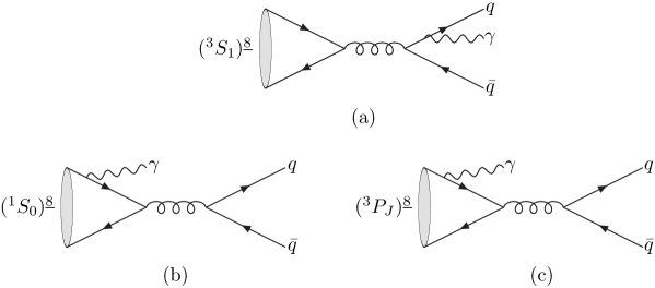
Figure 1: Feynman diagrams for transitions from color octet $b\bar{b}$ to color-octet $q\bar{q}$ (where $q=c$) by emitting a photon

II.1 General results

In the nonrelativistic approximation, the $\Upsilon$ radiative decay into a color-singlet $c\bar{c}$ pair, which subsequently hadronizes into charmonium, can be described by the diagrams in Fig.2, and the amplitude can be expressed asliu

$${\cal A}\Big{(}b\bar{b}({}^{3}S_{1})(2p_{b})\rightarrow c\bar{c}({}^{2S+1}L_{J})(2p_{c})\Big{)}=\sqrt{C_{L_{\Upsilon}}}\sqrt{C_{L}}\sum\limits_{L_{\Upsilon z}S_{\Upsilon z}}\sum\limits_{s_{1}s_{2}}\sum\limits_{jk}\sum\limits_{L_{z}S_{z}}\sum\limits_{s_{3}s_{4}}\sum\limits_{il}$$ (3)

$$\times \langle 1\mid\bar{3}k;3j\rangle\langle J_{\Upsilon}J_{\Upsilon z}\mid L_{\Upsilon}L_{\Upsilon z};S_{\Upsilon}S_{\Upsilon z}\rangle\langle S_{\Upsilon}S_{\Upsilon z}\mid s_{1};s_{2}\rangle$$

$$\times \langle s_{3};s_{4}\mid SS_{z}\rangle\langle LL_{z};SS_{z}\mid JJ_{z}\rangle\langle 3l;\bar{3}i\mid 1\rangle$$

$$\times \left\{\begin{array}[]{ll}{\cal A}\Big{(}b_{j}(p_{b})+\bar{b}_{k}(p_{b})\rightarrow\gamma(p_{3})+c_{l}(p_{c})+\bar{c}_{i}(p_{c})\Big{)}&(L=S),\\ \epsilon^{*}_{\alpha}(L_{Z}){\cal A}^{\alpha}\Big{(}b_{j}(p_{b})+\bar{b}_{k}(p_{b})\rightarrow\gamma(p_{3})+c_{l}(p_{c})+\bar{c}_{i}(p_{c})\Big{)}&(L=P),\end{array}\right.$$

where $\langle 3l;\bar{3}i\mid 1\rangle$$=\delta_{li}/\sqrt{N_{c}}$ ,  $\langle s_{1};s_{2}\mid SS_{z}\rangle$ , and $\langle LL_{z};SS_{z}\mid JJ_{z}\rangle$ are respectively the color-SU(3), spin-SU(2), and angular momentum Clebsch-Gordan coefficients for $Q\bar{Q}$ pairs projecting on appropriate bound states. ${\cal A}(b_{j}(p_{b})+\bar{b}_{k}(p_{b})\rightarrow Q_{l}(p_{c})+\bar{Q}_{i}(p_{c}))$ is the decay amplitude for $Q\bar{Q}$ production and ${\cal A}^{\alpha}$ is the derivative of the amplitude with respect to the relative momentum between the quark and anti-quark in the bound state. The coefficients $C_{L_{\Upsilon}}$ and $C_{L}$ can be related to the radial wave function of the bound states or its derivative with respect to the relative spacing as

$$C_{S}=\frac{1}{4\pi}|R_{s}(0)|^{2},\ \ \ C_{P}=\frac{3}{4\pi}|R_{p}^{\prime}(0)|^{2}.$$ (4)

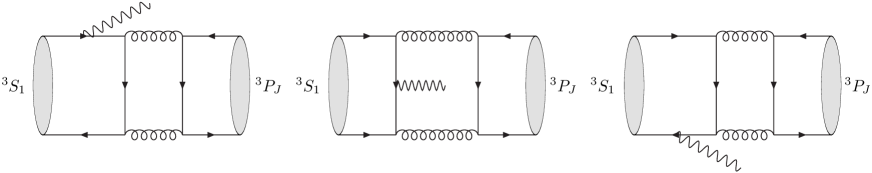
Figure 2: Typical QCD Feynman diagrams for heavy quarkonium (${}^{3}S_{1}$) radiative decays into (${}^{3}P_{J}$) mesons

The spin projection operators $P_{SS_{z}}(p,q)$ which describe production of quarkonium are expressed in terms of quark and anti-quark spinors asliu ; Kuhn :

$$P_{SS_{z}}(p,q)\!=\!\!\!\sum_{s_{1},s_{2}}\!\!v(\frac{p}{2}\!-\!q,\!s_{2})\bar{u}(\!\frac{p}{2}\!+\!q,\!s_{1})\!\langle s_{1};\!s_{2}|SS_{z}\!\rangle,$$ (5)

We list the spin projection operators and their derivatives with respect to the relative momentum, which will be used in the calculations, as

$$P_{00}(p,0) = \frac{1}{2\sqrt{2}}\gamma_{5}(\not{\!p}+2m),$$ (6)

$$P_{1S_{Z}}(p,0) = \frac{1}{2\sqrt{2}}\not{\epsilon}^{*}(S_{z})(\not{\!p}+2m),$$ (7)

$$P_{1S_{z}}^{\alpha}(p,0) = \frac{1}{4\sqrt{2}m}[\gamma^{\alpha}\not{\epsilon}^{*}(S_{z})(\not{\!p}+2m)-(\not{\!p}-2m)\not{\epsilon}^{*}(S_{z})\gamma^{\alpha}].$$ (8)

And the spin projection operators which describe the annihilation of quarkonium are the complex conjugate of the corresponding operators for production. The polarization vectors for the ${}^{3}P_{J}$ states are shown below:

$$\!\!\!\!\sum_{L_{Z}S_{Z}}\!\!\varepsilon^{\ast\alpha}\!(\!L_{z}\!)\epsilon^{\ast\beta}\!(\!S_{z}\!)\langle 1L_{z};\!1S_{z}|1J_{z}\rangle\! = \!\frac{-i\epsilon^{\alpha\beta\lambda\kappa}p_{\kappa}\epsilon_{\lambda}^{\ast}\!(\!J_{z}\!)}{\sqrt{2}M},$$ (9)

$$\!\!\!\!\sum_{L_{Z}S_{Z}}\!\!\varepsilon^{\ast\alpha}\!(\!L_{z}\!)\epsilon^{\ast\beta}\!(\!S_{z}\!)\langle 1L_{z};\!1S_{z}|0\,0\,\rangle\! = \!\!\frac{1}{\sqrt{3}}(-\!g^{\alpha\beta}\!+\!\frac{p^{\alpha}p^{\beta}}{M^{2}}\!),$$ (10)

$$\!\!\!\!\sum_{L_{Z}S_{Z}}\!\!\varepsilon^{\ast\alpha}\!(\!L_{z}\!)\epsilon^{\ast\beta}\!(\!S_{z}\!)\langle 1L_{z};\!1S_{z}|2J_{z}\rangle\! = \!\epsilon^{\ast\alpha\beta}(J_{z}),$$ (11)

where p is the momentum of P-wave quarkonium, and M is the mass of the corresponding quarkonium. $\epsilon_{\lambda}(J_{z})$ are the polarization vectors for $J=1$. $\epsilon^{\alpha\beta}(J_{z})$ are the polarization vectors for $J=2$, which are symmetric under the exchange $\alpha\leftrightarrow\!\beta$.

The QCD Feynman diagrams of $\Upsilon\to\gamma\eta_{c}(\chi_{cJ})$, in which the $c\bar{c}$ are produced through gluons, are shown in FIG.2, while the QED Feynman diagrams, in which the $c\bar{c}$ are produced through the photon, are shown in FIG.3. In the calculation, we use FeynCalc FeynCalc for the tensor reduction and LoopToolsLoopTools for the numerical evaluation of infrared safe integrals. We follow the way in Ref.fourrank to deal with five-point functions and high tensor loop integrals that can not be calculated by LoopTools and FeynCalc, such as

$$\!\!\!\!\!E_{\alpha\beta\rho\sigma} = \int\mathrm{{d}}^{D}k\frac{k_{\alpha}k_{\beta}k_{\rho}k_{\sigma}}{k^{2}[(k+p_{c})^{2}-m_{c}^{2}](k+2p_{c})^{2}[(p_{b}+k)^{2}-m_{b}^{2}][(k+2p_{c}-p_{b})^{2}-m_{b}^{2}]}.$$ (12)

where $p_{c}$ is the momentum of $c$ quark, $p_{b}$ the momentum of $b$ quark, $m_{c}$ the charm quark mass, and $m_{b}$ the bottom quark mass.

Figure 3: Typical QED Feynman diagrams for heavy quarkonium (${}^{3}S_{1}$) radiative decays into (${}^{3}P_{J}$) mesons

process	$\Upsilon\to\chi_{c2}\gamma$	$\Upsilon\to\chi_{c1}\gamma$	$\Upsilon\to\chi_{c0}\gamma$	$\Upsilon\to\eta_{c}\gamma$
$BR_{QCD}$	$5.1\times 10^{-6}$	$4.5\times 10^{-6}$	$4.0\times 10^{-6}$	$2.9\times 10^{-5}$
$BR_{QCD+QED}$	$5.6\times 10^{-6}$	$9.8\times 10^{-6}$	$3.2\times 10^{-6}$	$4.9\times 10^{-5}$
process	$\chi_{b2}\to J/\psi\gamma$	$\chi_{b1}\to J/\psi\gamma$	$\chi_{b0}\to J/\psi\gamma$	$\eta_{b}\to J/\psi\gamma$
$\Gamma_{QCD}$(GeV)	$2.7\times 10^{-10}$	$3.8\times 10^{-10}$	$5.0\times 10^{-10}$	$2.8\times 10^{-9}$
$\Gamma_{QCD+QED}$(GeV)	$3.6\times 10^{-10}$	$3.7\times 10^{-10}$	$1.3\times 10^{-10}$	$9.6\times 10^{-10}$
$\Gamma_{QED}$(GeV)	$3.8\times 10^{-11}$	$3.3\times 10^{-12}$	$1.3\times 10^{-10}$	$1.2\times 10^{-9}$

Table 1: Decay widths and branching ratios for radiative decays of bottomonium into charmonium. The decay widths $\Gamma$ are in units of GeV, and the branching ratios $BR$ are given for the $\Upsilon$.

In the numerical calculations, the quark masses are taken to be $m_{b}=4.7\,\mbox{GeV}$, $m_{c}=1.5\,\mbox{GeV}$, the wave functions at the origin can be found from potential model calculations in Ref.Quig : $|\mathcal{R}^{b\bar{b}}_{S}(0)|^{2}=6.477~{}$GeV³, $|\mathcal{R}^{c\bar{c}}_{S}(0)|^{2}=0.81~{}$GeV³, $|\mathcal{R}^{\prime b\bar{b}}_{P}(0)|^{2}=1.417~{}$GeV⁵, ${|\mathcal{R}^{\prime c\bar{c}}}_{P}(0)|^{2}=0.075~{}$GeV⁵. In the bottomonium decay, the strong coupling constant is chosen as $\alpha_{s}(2m_{b})=0.19$. The numerical results of radiative decays of bottomonium into charmonium are listed in Table I.

II.2 $\eta_{b}$ radiative decay to $J/\psi$

The $\eta_{b}$ meson is the only one among the low lying bottomonium states that has not been observed experimentally. To search for the $\eta_{b}$ meson a number of decay channels have been suggested, e.g., decays into the $J/\psi J/\psi$ and $D\overline{D}^{(*)}$ braaten ; maltoni ; jia . In any case, the radiative decay $\eta_{b}\to J/\psi\gamma$ should be a useful channel for the $\eta_{b}$ in view of the cleanness of the signal (this possibility has also been considered in Ref.hao ).

From Table I, we can see that for the $\eta_{b}$ decay $\eta_{b}\to J/\psi\gamma$ the QCD and QED contributions are comparable but destructive, and, as a result, the decay width of $\eta_{b}\to J/\psi\gamma$ is only $9.6\times 10^{-10}$ GeV. In order to know the branching ratio of this decay channel, we should have an estimate for the $\eta_{b}$ total width. In fact, we can estimate its total width through $\Gamma_{tot}(\eta_{b})\approx\Gamma(\eta_{b}\to gg)$ BBL . For $\Gamma(\eta_{b}\to gg)$, with next to leading order (NLO) QCD radiative corrections, we have

$$\Gamma(\eta_{b}\to gg)={|\mathcal{R}_{s}(0)|^{2}C_{F}\alpha_{s}^{2}(2m_{b})\over 2m_{b}^{2}}\Bigg{\{}1+\left[\left({\pi^{2}\over 4}-5\right)C_{F}+\left({199\over 18}-{13\pi^{2}\over 24}\right)C_{A}-{8\over 9}n_{f}\right]{\alpha_{s}\over\pi}\Bigg{\}}.$$ (13)

With the parameters used above, we can get $\Gamma_{tot}(\eta_{b})\approx 11.4$ MeV. Then the branching ratio is $Br(\eta_{b}\to\gamma J/\psi)\approx 8.4\times 10^{-8}$. If we use the leading order formula in Eq.(13), the decay width is $\Gamma_{tot}(\eta_{b})\approx 7.1~{}$MeV, and the branching ratio becomes $Br(\eta_{b}\to\gamma J/\psi)\approx 1.4\times 10^{-7}$.

On the other hand, with the spin symmetry in the nonrelativistic limit ($v=0$), the $\eta_{b}$ wave function at the origin $|\mathcal{R}_{s}(0)|^{2}$ can be determined from the $\Upsilon$ leptonic width,

$$\Gamma(\Upsilon\to e^{+}e^{-}) = N_{c}Q_{b}^{2}\alpha^{2}\frac{|\mathcal{R}_{s}(0)|^{2}}{3m_{b}^{2}}\left(1-\frac{16\alpha_{s}}{3\pi}\right),$$ (14)

and the $\eta_{b}$ total width is then related to the $\Upsilon$ leptonic width,

$$\Gamma_{tot}(\eta_{b})=\frac{3C_{F}\alpha_{s}^{2}(2m_{b})}{2N_{c}Q_{b}^{2}\alpha^{2}}\frac{1+\left[\left({\pi^{2}\over 4}-5\right)C_{F}+\left({199\over 18}-{13\pi^{2}\over 24}\right)C_{A}-{8\over 9}n_{f}\right]{\alpha_{s}\over\pi}}{1-\frac{16\alpha_{s}}{3\pi}}\Gamma(\Upsilon\to e^{+}e^{-}).$$ (15)

Using $m_{b}=4.7$ GeV, $\alpha_{s}(2m_{b})=0.19$, and experimental data $\Gamma(\Upsilon\to e^{+}e^{-})=1.340\pm 0.018$ KeVPdg , we can get $\Gamma_{tot}(\eta_{b})\approx 13.0$ MeV. Then the branching ratio is $Br(\eta_{b}\to\gamma J/\psi)\approx 7.3\times 10^{-8}$. If we use the leading order formula in Eq.(13) and Eq.(14), the $\Gamma_{tot}(\eta_{b})\approx 5.45~{}$MeV, the branching ratio is $Br(\eta_{b}\to\gamma J/\psi)\approx 1.7\times 10^{-7}$.

In any case, we find that the branching ratio $Br(\eta_{b}\to\gamma J/\psi)$ is of order $1\times 10^{-7}$. This small number makes it quite difficult to search for $\eta_{b}$ through this decay channel.

II.3 Helicity ratios with $\chi_{c1}$ and $\chi_{c2}$

We give predictions for branching ratios for different helicity states in $\Upsilon\to\chi_{cJ}\gamma$ decays. As in Ref. JPMa , we choose the moving direction of $\chi_{cJ}$ as the z-axis, and introduce three polarization vectors:

$$\omega^{\mu}(1) = \frac{-1}{\sqrt{2}}(0,1,i,0),\,\,\,$$

$$\omega^{\mu}(-1)\!\! = \!\!\frac{1}{\sqrt{2}}(0,1,-i,0)$$

$$\omega^{\mu}(0) = \frac{1}{m}(|\textbf{k}|,0,0,k^{0}),$$ (16)

thus we can characterize the tensor $\epsilon^{\mu\nu}(\lambda)$ of $\chi_{c2}$

$$\!\!\!\!\!\!\!\epsilon^{\alpha\beta}(2)\!\!\! = \!\!\!\omega^{\alpha}(1)\omega^{\beta}(1)$$

$$\!\!\!\!\!\!\!\epsilon^{\alpha\beta}(1)\!\!\! = \!\!\!\frac{1}{\!\!\sqrt{2}}(\omega^{\alpha}(1)\omega^{\beta}(0)+\omega^{\alpha}(0)\omega^{\beta}(1))$$

$$\!\!\!\!\!\!\epsilon^{\alpha\beta}(0)\!\!\! = \!\!\!\frac{1}{\!\!\sqrt{6}}(\omega^{\alpha}(-1)\omega^{\beta}(1)+2\omega^{\alpha}(0)\omega^{\beta}(0)+\omega^{\alpha}(1)\omega^{\beta}(-1))$$

$$\epsilon^{\alpha\beta}(-1)\!\!\! = \!\!\!\frac{1}{\!\!\sqrt{2}}(\omega^{\alpha}(0)\omega^{\beta}(-1)+\omega^{\alpha}(-1)\omega^{\beta}(0))$$

$$\epsilon^{\alpha\beta}(-2)\!\!\! = \!\!\!\omega^{\alpha}(-1)\omega^{\beta}(-1)$$ (17)

The helicity ratios are introduced as

$$\begin{split}x^{2}=\frac{|a_{1}|^{2}}{|a_{0}|^{2}}\text{ and }y^{2}=\frac{|a_{2}|^{2}}{|a_{0}|^{2}},\end{split}$$

where $a_{\lambda},\ \lambda=0,\ 1,\ 2,$ are the normalized helicity amplitudes, which satisfy $|a_{0}|^{2}+|a_{1}|^{2}+|a_{2}|^{2}=1$. Namely, $|a_{\lambda}|^{2}$ is the probability of the final state meson with helicity $\pm\lambda$. Then the ratios $x^{2}$ and $y^{2}$ only depend on the mass ratio $m_{c}/m_{b}$. With the same choice of parameters, we predict ratios for different helicities in Table II.

	QCD	QCD+QED		QCD	QCD+QED
$x^{2}(\Upsilon\to\gamma\chi_{c2})$	0.37	0.38	$x^{2}(\Upsilon\to\gamma\chi_{c1})$	0.064	0.075
$y^{2}(\Upsilon\to\gamma\chi_{c2})$	0.14	0.14

Table 2: Results for $\Upsilon\to\chi_{cJ}\gamma(J=1,2)$ with different helicity states

III Radiative decays of heavy quarkonium into light mesons

As a purely phenomenological model-dependent study, In this section we will extend our calculations performed above for radiative decays of bottomonia into charmonia to the radiative decays of bottomonia into light mesons. Our assumption is that the light mesons such as the $f_{2}(1270)$, $f_{2}^{\prime}(1525)$, and $f_{1}(1285)$ can be described by nonrelativistic $q\bar{q}~{}(q=u,d,s)$ bound states with constituent quark masses.

In the numerical calculations, the light quark masses are taken to be $m_{s}=0.50\,\mbox{GeV}$, $m_{u}=m_{d}=0.35\,\mbox{GeV}$. The parameters for the heavy quarks are the same as that used in section II,$|\mathcal{R}^{b\bar{b}}_{S}(0)|^{2}=6.477~{}$GeV³, $|\mathcal{R}^{c\bar{c}}_{S}(0)|^{2}=0.81~{}$GeV³, $|\mathcal{R}^{\prime b\bar{b}}_{P}(0)|^{2}=1.417~{}$GeV⁵, $|\mathcal{R}^{\prime c\bar{c}}_{P}(0)|^{2}=0.075~{}$GeV⁵, $m_{b}=4.7~{}$GeV, and $m_{c}=1.5~{}$GeV. The strong coupling constant is chosen as $\alpha_{s}=0.19$ and $\alpha_{s}=0.26$ in bottomonium and charmonium decays respectively.

As widely accepted assignments we assume that $f_{2}(1270)$ and $f_{1}(1285)$ are mainly composed of $(u\bar{u}+d\bar{d})/\sqrt{2}$ (neglecting the mixing with $s\bar{s}$ for simplicity). But for $f_{0}(980)$, there are many possible assignments such as the tetraquark state, the $K\bar{K}$ molecule, and the P-wave $s\bar{s}$ dominated state (for related discussions on $f_{0}(980)$ and other scalar mesons, see, e.g., the topical review–note on scalar mesons in Pdg and close ). Since experimental data show that $D_{s}^{+}\to f_{0}(980)\pi^{+}$ has a large branching ratio (BR)Pdg , here we assign $f_{0}(980)$ as an $s\bar{s}$ dominated P-wave state as a tentative choice (we do not try to justify this assignment).

As to the wave functions at the origin of light mesons, it is very difficult to determine them without any doubt. Using the theoretical expression for the widths of $f_{2}\to\gamma\gamma$BBL ,

$$\Gamma_{f_{2}(1270)\to\gamma\gamma}^{(th)} = \frac{6N_{c}}{5}(Q_{u}^{2}+Q_{d}^{2})^{2}\alpha^{2}\frac{|\mathcal{R}^{\prime}_{P}(0)|^{2}}{m^{4}}(1-\frac{8\alpha_{s}}{3\pi})^{2}$$

$$\Gamma_{f_{2}^{\prime}(1525)\to\gamma\gamma}^{(th)} = \frac{12N_{c}}{5}Q_{s}^{4}\alpha^{2}\frac{|\mathcal{R}^{\prime}_{P}(0)|^{2}}{m^{4}}(1-\frac{8\alpha_{s}}{3\pi})^{2},$$ (18)

where $N_{c}$=3 is the color number, $\alpha=1/137$, and fitting them with their experimental values 2.6 KeV and 0.081 KeV for $f_{2}(1270)$ and $f_{2}^{\prime}(1525)$ respectivelyPdg , we get

$$|\mathcal{R}^{\prime n\bar{n}}_{P}(0)|^{2} = 1.58\times 10^{-3}\,\,\mbox{GeV}^{5},$$

$$|\mathcal{R}^{\prime s\bar{s}}_{P}(0)|^{2} = 2.23\times 10^{-3}\,\,\mbox{GeV}^{5}.$$ (19)

If we use the leading order formula in Eq(III), then

$$|\mathcal{R}^{\prime n\bar{n}}_{P}(0)|^{2} = 6.6\times 10^{-4}\,\,\mbox{GeV}^{5}$$

$$|\mathcal{R}^{\prime s\bar{s}}_{P}(0)|^{2} = 1.1\times 10^{-3}\,\,\mbox{GeV}^{5}.$$ (20)

For the vector mesons, the wave functions at the origin may be determined from their leptonic decay $V\to e^{+}e^{-}$  ($V=\phi,\rho$) widths. Using

$$\Gamma(\phi(1020)\to e^{+}e^{-}) = N_{c}Q_{s}^{2}\alpha^{2}\frac{|\mathcal{R}(0)|^{2}}{3m_{s}^{2}}(1-\frac{8\alpha_{s}}{3\pi})^{2}=(1.27\pm 0.04)~{}\mbox{KeV},$$ (21)

we can get

$$|\mathcal{R}^{n\bar{n}}_{S}(0)|^{2} = 0.11\,\,\mbox{GeV}^{3},\hskip 28.45274pt$$

$$|\mathcal{R}^{s\bar{s}}_{S}(0)|^{2} = 0.19\,\,\mbox{GeV}^{3}.$$ (22)

If we use the leading order formula in Eq.(21), then

$$|\mathcal{R}^{n\bar{n}}_{S}(0)|^{2} = 0.032\,\,\mbox{GeV}^{3},\hskip 28.45274pt$$

$$|\mathcal{R}^{s\bar{s}}_{S}(0)|^{2} = 0.054\,\,\mbox{GeV}^{3}.$$ (23)

The wave functions at the origin of light mesons can also be determined from potential models Quigg:1979vr . From experimental data, $\Delta E=M(2S)-M(1S)$ is $675~{}$MeV, $638~{}$MeV, $661~{}$MeV, $589~{}$MeV, and $563~{}$MeV for $\rho$, $\omega$, $\phi$, $J/\psi$, and $\Upsilon$ respectively. In the logarithmic potential, $\Delta E$ is independent of quark masses. So we may select the logarithmic potential, which gives

$$|R_{S}(0)|^{2} \propto m_{q}^{3/2}$$

$$|R_{P}(0)|^{2} \propto m_{q}^{5/2}$$ (24)

With $|\mathcal{R}^{c\bar{c}}_{S}(0)|^{2}=0.81~{}$GeV³ and $|\mathcal{R}^{\prime c\bar{c}}_{P}(0)|^{2}=0.075~{}$GeV⁵ . Then we can get

$$|\mathcal{R}^{n\bar{n}}_{S}(0)|^{2} = \left(\frac{m_{n}}{m_{c}}\right)^{3/2}|\mathcal{R}^{c\bar{c}}_{S}(0)|^{2}=0.091\mbox{GeV}^{3}$$

$$|\mathcal{R}^{s\bar{s}}_{S}(0)|^{2} = \left(\frac{m_{s}}{m_{c}}\right)^{3/2}|\mathcal{R}^{c\bar{c}}_{S}(0)|^{2}=0.156\mbox{GeV}^{3}$$

$$|\mathcal{R}^{\prime n\bar{n}}_{P}(0)|^{2} = \left(\frac{m_{n}}{m_{c}}\right)^{5/2}|\mathcal{R}^{\prime c\bar{c}}_{P}(0)|^{2}=1.97\times 10^{-3}\mbox{GeV}^{5}$$

$$|\mathcal{R}^{\prime s\bar{s}}_{P}(0)|^{2} = \left(\frac{m_{s}}{m_{c}}\right)^{5/2}|\mathcal{R}^{\prime c\bar{c}}_{P}(0)|^{2}=4.81\times 10^{-3}\mbox{GeV}^{5}$$ (25)

In the numerical calculation, the parameters are taken to be $|\mathcal{R}^{s\bar{s}}_{S}(0)|^{2}=0.054~{}$GeV³, $|\mathcal{R}^{n\bar{n}}_{S}(0)|^{2}=0.032~{}$GeV³, $|\mathcal{R}^{\prime s\bar{s}}_{P}(0)|^{2}=1.1\times 10^{-3}~{}$GeV⁵, $|\mathcal{R}^{\prime n\bar{n}}_{P}(0)|^{2}=6.6\times 10^{-4}~{}$GeV⁵. The numerical results are shown in Table III and Table IV.

process	$\Upsilon\to\gamma f_{0}(n\bar{n})$	$\Upsilon\to\gamma f_{1}(1285)$	$\Upsilon\to\gamma f_{2}(1270)$	$\Upsilon\to\gamma f_{0}(980)$	$\Upsilon\to\gamma f_{1}^{\prime}(1420)$	$\Upsilon\to\gamma f_{2}^{\prime}(1525)$
$BR_{th}^{QCD}$	$7.2\times 10^{-5}$	$2.6\times 10^{-5}$	$7.1\times 10^{-5}$	$2.2\times 10^{-5}$	$1.0\times 10^{-5}$	$2.2\times 10^{-5}$
$BR_{th}^{QCD+QED}$	$6.4\times 10^{-5}$	$3.9\times 10^{-5}$	$6.3\times 10^{-5}$	$2.0\times 10^{-5}$	$1.2\times 10^{-5}$	$2.0\times 10^{-5}$
$BR_{ex}$	$\backslash$	$\backslash$	$1.00\pm 0.10\times 10^{-4}$	$<3\times 10^{-5}$	$\backslash$	$3.7^{+1.2}_{-1.1}\times 10^{-5}$
process	$J/\psi\to\gamma f_{0}(n\bar{n})$	$J/\psi\to\gamma f_{1}(1285)$	$J/\psi\to\gamma f_{2}(1270)$	$J/\psi\to\gamma f_{0}(980)$	$J/\psi\to\gamma f_{1}^{\prime}(1420)$	$J/\psi\to\gamma f_{2}^{\prime}(1525)$
$BR_{th}^{QCD}$	$2.0\times 10^{-3}$	$2.0\times 10^{-3}$	$2.5\times 10^{-3}$	$6.7\times 10^{-4}$	$7.5\times 10^{-4}$	$8.5\times 10^{-4}$
$BR_{th}^{QCD+QED}$	$1.8\times 10^{-3}$	$2.7\times 10^{-3}$	$2.4\times 10^{-3}$	$6.5\times 10^{-4}$	$8.5\times 10^{-4}$	$8.5\times 10^{-4}$
$BR_{ex}$	$\backslash$	$(6.1\pm 0.8)\times 10^{-4}$	$(13.8\pm 1.4)\times 10^{-4}$	$\backslash$	$(7.9\pm 1.3)\times 10^{-4}$	$(4.5^{+0.7}_{-0.4})\times 10^{-4}$

Table 3: Numerical results for $\Upsilon(J/\psi)\to\gamma f_{J}$ .

process	$\chi_{b2}\to\gamma\rho$	$\chi_{b1}\to\gamma\rho$	$\chi_{b0}\to\gamma\rho$	$\eta_{b}\to\gamma\rho$
$\Gamma_{QCD}$(GeV)	$1.1\times 10^{-10}$	$2.2\times 10^{-10}$	$3.5\times 10^{-11}$	$1.2\times 10^{-10}$
$\Gamma_{QCD+QED}$(GeV)	$6.8\times 10^{-10}$	$2.2\times 10^{-10}$	$8.4\times 10^{-10}$	$1.1\times 10^{-8}$
process	$\chi_{b2}\to\gamma\omega$	$\chi_{b1}\to\gamma\omega$	$\chi_{b0}\to\gamma\omega$	$\eta_{b}\to\gamma\omega$
$\Gamma_{QCD}$(GeV)	$1.2\times 10^{-11}$	$2.4\times 10^{-11}$	$3.8\times 10^{-12}$	$1.3\times 10^{-11}$
$\Gamma_{QCD+QED}$(GeV)	$7.6\times 10^{-11}$	$2.4\times 10^{-11}$	$9.3\times 10^{-11}$	$1.2\times 10^{-9}$
process	$\chi_{b2}\to\gamma\phi$	$\chi_{b1}\to\gamma\phi$	$\chi_{b0}\to\gamma\phi$	$\eta_{b}\to\gamma\phi$
$\Gamma_{QCD}$(GeV)	$3.6\times 10^{-11}$	$5.8\times 10^{-11}$	$1.6\times 10^{-11}$	$5.9\times 10^{-11}$
$\Gamma_{QCD+QED}$(GeV)	$1.3\times 10^{-10}$	$5.8\times 10^{-11}$	$7.5\times 10^{-11}$	$1.2\times 10^{-9}$
process	$\chi_{c2}\to\gamma\rho$	$\chi_{c1}\to\gamma\rho$	$\chi_{c0}\to\gamma\rho$	$\eta_{c}\to\gamma\rho$
$BR_{th}^{QCD}$	$1.3\times 10^{-5}$	$4.1\times 10^{-5}$	$3.2\times 10^{-6}$	$1.5\times 10^{-6}$
$BR_{th}^{QCD+QED}$	$3.8\times 10^{-5}$	$4.2\times 10^{-5}$	$2.0\times 10^{-6}$	$4.5\times 10^{-6}$
process	$\chi_{c2}\to\gamma\omega$	$\chi_{c1}\to\gamma\omega$	$\chi_{c0}\to\gamma\omega$	$\eta_{c}\to\gamma\omega$
$BR_{th}^{QCD}$	$1.5\times 10^{-6}$	$4.6\times 10^{-6}$	$3.5\times 10^{-7}$	$1.7\times 10^{-7}$
$BR_{th}^{QCD+QED}$	$4.2\times 10^{-6}$	$4.7\times 10^{-6}$	$2.2\times 10^{-7}$	$5.0\times 10^{-7}$
process	$\chi_{c2}\to\gamma\phi$	$\chi_{c1}\to\gamma\phi$	$\chi_{c0}\to\gamma\phi$	$\eta_{c}\to\gamma\phi$
$BR_{th}^{QCD}$	$3.3\times 10^{-6}$	$1.1\times 10^{-5}$	$1.3\times 10^{-6}$	$7.1\times 10^{-7}$
$BR_{th}^{QCD+QED}$	$6.5\times 10^{-6}$	$1.1\times 10^{-5}$	$3.0\times 10^{-8}$	$4.0\times 10^{-7}$

Table 4: Predicted decay widths for $\chi_{bJ}(\eta_{b})\to\gamma\rho(\omega,\phi)$.

The branching ratio of $\Upsilon$ radiative decay into a light meson is smaller than the corresponding branching ratio of $J/\psi$ by a factor of

$$\frac{BR(\Upsilon\to\gamma\ M)}{BR(J/\psi\to\gamma\ M)}\sim\left(\frac{Q_{b}}{Q_{c}}\right)^{2}\left(\frac{m_{c}}{m_{b}}\right)^{2}\frac{\alpha(2m_{b})}{\alpha(2m_{c})}\sim 0.02$$ (26)

We can find this theoretical ratio is $0.013\sim 0.036$. The experimental ratio is 0.072 for $f_{2}(1270)$, and 0.082 for $f_{2}^{\prime}(1525)$. The corresponding theoretical ratios are $0.026$ and $0.024$ for $f_{2}(1270)$ and $f_{2}^{\prime}(1525)$ respectively. If we use larger constituent quark masses, e.g. $m_{u}=m_{d}=M(1270)/2$, $m_{s}=M(1525)/2$, the ratios are $0.018$ and $0.018$ for $f_{2}(1270)$ and $f_{2}^{\prime}(1525)$ respectively.

With the same parameters, we give the branching ratios for different helicity states in Table V. The corresponding values of helicity parameters $x$ and $y$ are $x=0.46$, $y=0.23$. Recently, new experimental data for the contributions of different helicities in process $J/\psi\to\gamma f_{2}(1270)$ have been given by the BES Collaboration besjpsi: $x=0.89\pm 0.02\pm 0.10$ and $y=0.46\pm 0.02\pm 0.17$ (see alsoPdg ). It is about 2 times larger than our results. But if we use a larger constituent quark mass, e.g. $m_{u}=M(1270)/2$, we will get substantially increased values $x=0.79$ and $y=0.58$ (also see Ref.kor ). We emphasize that the helicity parameters are very sensitive to the light quark masses, and hence very useful in clarifying the decay mechanisms. Note that if $m_{u}/m_{c}\to 0$, we will have $x\to 0$ and $y\to 0$, but this is inconsistent with data.

$m_{q}$(GeV)		QCD	QCD+QED		QCD	QCD+QED		QCD	QCD+QED
0.35	$x^{2}(\Upsilon\to\gamma f_{2})$	0.023	0.023	$y^{2}(\Upsilon\to\gamma f_{2})$	0.0013	0.0014	$x^{2}(\Upsilon\to\gamma f_{1})$	0.00069	0.00010
0.635	$x^{2}(\Upsilon\to\gamma f_{2})$	0.073	0.075	$y^{2}(\Upsilon\to\gamma f_{2})$	0.0095	0.010	$x^{2}(\Upsilon\to\gamma f_{1})$	0.0047	0.0067
0.50	$x^{2}(\Upsilon\to\gamma f_{2}^{\prime})$	0.045	0.046	$y^{2}(\Upsilon\to\gamma f_{2}^{\prime})$	0.0043	0.0045	$x^{2}(\Upsilon\to\gamma f_{1}^{\prime})$	0.0018	0.0023
0.763	$x^{2}(\Upsilon\to\gamma f_{2}^{\prime})$	0.10	0.11	$y^{2}(\Upsilon\to\gamma f_{2}^{\prime})$	0.017	0.018	$x^{2}(\Upsilon\to\gamma f_{1}^{\prime})$	0.0087	0.010
0.35	$x^{2}(J/\psi\to\gamma f_{2})$	0.21	0.21	$y^{2}(J/\psi\to\gamma f_{2})$	0.055	0.057	$x^{2}(J/\psi\to\gamma f_{1})$	0.026	0.029
0.635	$x^{2}(J/\psi\to\gamma f_{2})$	0.62	0.62	$y^{2}(J/\psi\to\gamma f_{2})$	0.33	0.33	$x^{2}(J/\psi\to\gamma f_{1})$	0.13	0.14
0.50	$x^{2}(J/\psi\to\gamma f_{2}^{\prime})$	0.40	0.40	$y^{2}(J/\psi\to\gamma f_{2}^{\prime})$	0.16	0.16	$x^{2}(J/\psi\to\gamma f_{1}^{\prime})$	0.072	0.074
0.763	$x^{2}(J/\psi\to\gamma f_{2}^{\prime})$	0.86	0.86	$y^{2}(J/\psi\to\gamma f_{2}^{\prime})$	0.57	0.57	$x^{2}(J/\psi\to\gamma f_{1}^{\prime})$	0.21	0.22

Table 5: Results for $\Upsilon\to\chi_{cJ}\gamma$ with different helicity states

IV Summary

In this paper, we mainly investigate the radiative decays of bottomonium into charmonium, such as $\Upsilon\to\chi_{cJ}\gamma$, $\chi_{bJ}\to J/\psi\gamma$, $\eta_{b}\to J/\psi\gamma$ and $\Upsilon\to\eta_{c}\gamma$ based on the NRQCD approach. Based on our numerical calculations, we predict that the branching ratios of $\Upsilon\to\chi_{cJ}\gamma$ and decay widths of $\chi_{bJ}\to J/\psi\gamma$. All the above processes are perturbative calculable, and it is a good way to test NRQCD.

We next focus on the cases of heavy quarkonium radiative decays into light mesons, including $\Upsilon(J/\psi)\to f_{J}\gamma$ and $\chi_{bJ}\to\rho(\omega,\phi)\gamma$ et ac.

In this work, we also find that the QED effects in some radiative processes are really significant. For $\Upsilon\to\gamma\chi_{cJ}$ decay, the pure electromagnetic process only affects the final results for $J=0,2$ a little, but for the $J=1$ state the result may change by a factor of 2. The same results will be seen in the decays of $\Upsilon\to\gamma f_{J}$ and $J/\psi\to\gamma f_{J}$. As the cases of $\chi_{bJ}$ decays, especially for the process $\chi_{bJ}\to\rho(\omega,\phi)\gamma$, QED process may give dominant contributions.

References

• (1) G.Β T. Bodwin, E. Braaten and G.Β P. Lepage, Phys.Β Rev.Β D 51 , 1125 (1995); 55, 5853(E) (1997).
• (2) J.G. K$\ddot{o}$rner, J.H. K$\ddot{u}$hn, and H. Schneider, Phys. Lett. B 120, 444 (1983); J.G. K$\ddot{o}$rner , J.H. K$\ddot{u}$hn, M. Krammer, and H. Schneider, Nucl. Phys. B 229, 115 (1983).
• (3) M. Krammer, P​h​y​s.L​e​t​t.formulae-sequenceπ‘ƒβ„Žπ‘¦π‘ πΏπ‘’π‘‘π‘‘Phys.\ Lett. B 74, 361 (1978); J.G. Korner and M. Krammer, Z. Phys. C 16, 279 (1983).
• (4) Y.J. Gao, Y.J. Zhang and K.T. Chao, Chin. Phys. Lett. 23, 2376 (2003) (hep-ph/0607278).
• (5) Y.J. Gao, Y.J. Zhang, and K.T. Chao, Commun. Theor. Phys. 46, 1017 (2006) (hep-ph/0606170).
• (6) P. Cho and A.K. Leibovich, Phys. Rev. D53, 150 (1996); 53, 6203 (1996); P. Ko, J. Lee and H.S. Song, Phys. Rev. D54, 4312 (1996); K.Y. Liu, Z.G. He, K.T. Chao, Phys. Lett. B557, 45 (2003).
• (7) J. H. KΓΌhn, Nucl. Phys. B 157, 125 (1979); B. Guberina et al., Nucl. Phys. B 174, 317 (1980).
• (8) R. Mertig, M. BΓΆhm, A. Denner, Comput.Β Phys.Β Commun.Β 64 (1991) 345.
• (9) T. Hahn, M. Perez-Victoria, Comput.Β Phys.Β Commun.Β 118 (1999) 153.
• (10) A. Denner, S. Dittmaier, Nucl.Phys. B658 (2003) 175; A. Denner, S. Dittmaier, hep-ph/0509141.
• (11) E.J. Eichten and C. Quigg, Phys.Β Rev.Β D 52, 1726 (1995).
• (12) J.P. Ma, Nucl.Β Phys.Β  B 605 625 (2001); Erratum-ibid.Β  B611 523(2001).
• (13) S.Β B.Β Athar et al. [CLEO Collaboration], Phys.Β Rev.Β D 73, 032001 (2006) [arXiv:hep-ex/0510015].
• (14) S. Eidelman, et al. [Particle Data Group], Phys. Lett. B 592 (2004) 1; W.Β M.Β Yao et al. [Particle Data Group], J.Β Phys.Β G 33, 1 (2006).
• (15) E. Braaten, S. Fleming, and A.K. Leibovich, Phys. Rev. D63, 094006 (2001).
• (16) F. Maltoni and A.D. Polosa, Phys. Rev. D70, 054014 (2004).
• (17) Y. Jia, hep-ph/0611130.
• (18) G. Hao, Y. Jia, C.F. Qiao, and P. Sun, hep-ph/0612173.
• (19) F.E. Close, G.R. Farrar, and Z.P. Li, Phys. Rev. D 55, 5749 (1997).
• (20) C.Β Quigg and J.Β L.Β Rosner, Phys.Β Rept.Β  56, 167 (1979).