$SU(3)$ Family Gauge Symmetry and the Axion

Abstract

We analyze the structure of a recently proposed effective field theory (EFT) for the generation of quark and lepton mass ratios and mixing angles, based on the spontaneous breaking of an $SU(3)$ family gauge symmetry at a high scale $F$. We classify the Yukawa operators necessary to seed the masses, making use of the continuous global symmetries that they preserve. One global $U(1)$, in addition to baryon number and electroweak hypercharge, remains unbroken after the inclusion of all operators required by standard-model-fermion phenomenology. An associated vacuum symmetry insures the vanishing of the first-family quark and charged-lepton masses in the absence of the family gauge interaction. If this $U(1)$ symmetry is taken to be exact in the EFT, broken explicitly by only the QCD-induced anomaly, and if the breaking scale $F$ is taken to lie in the range $10^{9}-10^{12}$ GeV, then the associated Nambu-Goldstone boson is a potential QCD axion.

I Introduction

In a recent set of papers APY2  APY3 , we developed an effective-field-theory (EFT) framework for the computation of quark and lepton masses and mixing angles based on an $SU(3)_{F}$ family gauge symmetry. The largest elements of the quark and charged-lepton mass matrices are seeded phenomenologically through a set of Yukawa operators, bilinear in the quark and lepton fields and including the Higgs doublet. They also include standard-model (SM)-singlet scalars transforming as sextets under the $SU(3)_{F}$ family group. The family symmetry is broken spontaneously at a high scale $F$ by vacuum expectation values (VEV’s) of these scalars. The $SU(3)_{F}$ family symmetry is realized nonlinearly among the SM-singlet scalars, so that only Nambu-Goldstone (NGB) and pseudo-Nambu-Goldstone (PNGB) degrees of freedom remain in the EFT.

The small charged-lepton mass ratios, and the small up-type and down-type quark mass ratios and Cabibbo-Kobayashi-Maskawa (CKM) mixing angles are then computed perturbatively in the family gauge coupling. Small, hierarchical neutrino masses, and large leptonic mixing angles are naturally accommodated at zeroth order in the family gauge coupling, although the specific values of the mixing angles are not predicted  APY3 . Imposing the constraints from the measured solar and atmospheric mass differences and mixing angles restricts the parameters describing the vacuum symmetry structure and can relate some of the otherwise free parameters in the quark and charged-lepton mass-matrix estimates. One small leptonic mixing angle then emerges, and is predicted to lie within the reach of planned experiments.

To classify the Yukawa operators of the EFT, we found it helpful in Refs. APY2  APY3 to make use of a discrete, $Z_{3}$, symmetry. Here we dispense with the $Z_{3}$ and show that a complete classification scheme is provided through the set of global $U(1)$ symmetries associated with each of the complex fields of the model. One combination is rendered anomalous by the $SU(3)_{F}$ family gauge interaction. We show that the dominant Yukawa operators required to describe (with the family gauge interactions) most features of the quark and charged-lepton mass matrices then preserve two $U(1)$ symmetries in addition to those associated with baryon number and electroweak hypercharge.

In order to fit precisely the quark and charged-lepton mass matrices, and to generate the neutrino mass matrix, it is necessary to include some additional, smaller operators that explicitly break these two $U(1)$ symmetries to one. This final symmetry, $U(1)_{a}$, is broken spontaneously at the scale $F$. If it is taken to be exact in the EFT, broken explicitly by only QCD anomalies, it could play the role of a Peccei-Quinn symmetry to address the strong CP problem PQ .

We first discuss the model and the Yukawa operators necessary to seed the quark and lepton mass matrices. We then describe the approximate global symmetries of the EFT, broken explicitly by the family gauge interactions and the Yukawa operators. We discuss the vacuum structure of the EFT, enumerating the NGB’s and PNGB’s, and then classify the fermion mass matrices that emerge from the Yukawa operators. We conclude with a discussion of the $U(1)_{a}$ global symmetry of the EFT, broken explicitly by QCD anomalies, and leading to a potential axion axion .

II The Model

The model of Refs. APY2  APY3 consists of the three families of SM fermions, together with two additional fermions, $\chi$ and $\chi^{c}$, also coming in three families, required to explain the up-type quark mass ratios. Each of the (left-handed, chiral) fermion fields, $q,u^{c},d^{c},\chi,\chi^{c},l,e^{c}$, transforms as a $\bf{3}$ under a family $SU(3)_{1}$ symmetry. Two complex, symmetric-tensor fields $S$ and $\Sigma$ ($\bf{\bar{6}}$’s) are employed to seed the spontaneous breaking of the $SU(3)_{1}$. These fields constitute the “visible” sector of the model. With electroweak symmetry breaking described by a single Higgs-doublet field, some additional mechanism is required to stabilize the Higgs mass. This problem was not addressed in Refs. APY2  APY3 , and will not be addressed here.

In order to compute the small quark mass ratios $m_{d}/m_{b}$, $m_{s}/m_{b}$, $m_{u}/m_{t}$, $m_{c}/m_{t}$, and the CKM mixing angles radiatively in the family gauge interaction, these quantities must vanish in its absence. To this end, a “hidden sector” is introduced transforming according to its own $SU(3)_{2}$. The $SU(3)_{F}$ family gauge interaction then arises from gauging the diagonal subgroup of $SU(3)_{1}\times SU(3)_{2}$.

The family breaking scale $F$ is taken to be large enough to suppress flavor-changing neutral currents, and the family gauge coupling $g$ is weak enough so that the gauge-boson masses, of order $gF$, are small compared to the cut-off $M_{F}=4\pi F$ of the EFT. Their effects can therefore be computed perturbatively within the EFT. The vanishing of the above mass ratios and the CKM angles in the absence of the family gauge interaction follows from the symmetries and vacuum structure in the visible sector. These symmetries are then broken in the hidden sector, with the breaking communicated to the visible sector through the gauge interactions, leading to nonzero, calculable values for the mass ratios and CKM angles.

The matter-field content of the EFT is summarized in Table 1. The hidden sector is described by a single complex, symmetric tensor field $H$, transforming as a $\bf{\bar{6}}$ under $SU(3)_{2}$. Note that no SM-singlet neutrinos are included in the EFT. If they exist, they are taken to have masses above the cutoff $M_{F}$, and have been integrated out. The EFT includes the fermion fields, the NGB and PNGB components of $S$, $\Sigma$ and $H$, the family gauge fields, and SM gauge fields.

The $SU(3)_{F}$ family gauge interaction is, so far, anomalous, requiring the existence of additional heavy fermions to remove the anomalies. An example is a set of three SM-singlet fermions, each transforming as a $\bf{\bar{6}}$ under $SU(3)_{2}$. With these “hidden-sector” fermions coupled to $H$, they all become massive when $H$ develops its symmetry-breaking VEV of order $F$. If their Yukawa couplings are strong ($O(4\pi)$), then the masses will be $O(M_{F}=4\pi F)$, and they will not be part of the EFT. When integrated out, they generate an appropriate Wess-Zumino-Witten (WZW) term at energies below $M_{F}$  WZW . It must be included in the EFT, but it does not affect the mass estimates of Refs. APY2  APY3 to leading order.

	$SU(3)_{1}$	$SU(3)_{2}$	$SU(3)_{c}$	$SU(2)_{L}$	$U(1)_{Y}$
$q$	3	1	3	2	$\frac{1}{6}$
$u^{c}$	3	1	$\bar{3}$	1	$-\frac{2}{3}$
$d^{c}$	3	1	$\bar{3}$	1	$\frac{1}{3}$
$\chi$	3	1	3	1	$\frac{2}{3}$
$\chi^{c}$	3	1	$\bar{3}$	1	$-\frac{2}{3}$
$\ell$	3	1	1	2	$-\frac{1}{2}$
$e^{c}$	3	1	1	1	1
$h$	1	1	1	2	$-\frac{1}{2}$
$S$	$\bar{6}$	1	1	1	0
$\Sigma$	$\bar{6}$	1	1	1	0
$H$	1	$\bar{6}$	1	1	0

Table 1: Field content and symmetries of the model. All fermions are LH chiral fields. The symbols $S$, $\Sigma$, and $H$ denote SM-singlet scalar fields.

III Yukawa Operators of the EFT, and $U(1)$ symmetries

III.1 Dominant Yukawa Operators

In the absence of the Yukawa operators, there exists a $U(1)$ global symmetry for each of the $11$ complex fields of Table 1. A minimal set of Yukawa operators required to seed most features of the quark- and charged-lepton mass matrices is given by

$$-{\cal L}_{Y} = y_{d}\frac{qhSd^{c}}{F}+y_{1}\frac{q\tilde{h}S\chi^{c}}{F}+y_{2}\chi Su^{c}+y_{3}\chi\Sigma\chi^{c}$$ (1)

$$+y_{e}\frac{\ell hSe^{c}}{F}+{\rm h.c.}.$$

The dimensionless coupling constants, fit to experiment, range in size from $O(10^{-3})$ to $O(1)$, with electroweak symmetry breaking arising from the Higgs VEV $v\simeq 250$ GeV. The VEV’s of $S$ and $\Sigma$ are of order $F$. (The $H$ field, so far not directly coupled to the visible sector, also develops a VEV of order $F$.) The first and last terms seed the largest elements of the down-type and charged-lepton mass matrices. The other three terms are required to set up a (“see-saw”) mass-generating mechanism in the up-type sector APY2 . All these operators are dimension-$3$ or $4$ in the fields with SM quantum numbers.

The phenomenological consequences of these operators were analyzed in Refs. APY2  APY3 . There are many other Yukawa operators allowed by the SM symmetries and the $SU(3)_{F}$ gauge symmetry, especially since the $SU(3)_{F}$ symmetry is realized nonlinearly in the scalar ($S$, $\Sigma$, and $H$) sectors. In order to justify using only these operators we will make use of the $U(1)$ symmetries that are naturally part of the model.

The $5$ operators of ${\cal L}_{Y}$ break $5$ of the $10$ $U(1)$ symmetries associated with the visible-sector fields of Table 1. In addition, one combination, which can be taken to be lepton number, $U(1)_{\ell}$, is rendered anomalous by the $SU(3)_{F}$ family gauge interaction. Of the remaining $4$ $U(1)$’s, $2$ are $U(1)_{B}$ corresponding to baryon number and $U(1)_{Y}$ corresponding electroweak hypercharge. The final $2$ are denoted $U(1)_{a}$ and $U(1)_{b}$. We exhibit in Table 2 one possible choice for the charge assignments of each of the complex fields under $U(1)_{a}\times U(1)_{b}$. The reason for the charge assignments of $H$ will be made clear shortly.

We will show using the vacuum structure of the EFT that the operators of ${\cal L}_{Y}$ provide the required dominant seeding of the quark and charged-lepton mass matrices, that is, that other Yukawa operators respecting the $U(1)_{a}\times U(1)_{b}$ symmetry provide no new mass-matrix structure.

	$q$	$u^{c}$	$d^{c}$	$\chi$	$\chi^{c}$	$\ell$	$e^{c}$	$h$	$S$	$\Sigma$	$H$
$U(1)_{a}$	0	0	2	1	0	-11	13	-1	-1	-1	20
$U(1)_{b}$	1	0	0	0	-2	-1	2	-1	0	2	0

Table 2: Two linearly independent $U(1)$’s, in addition to $U(1)_{B}$ and $U(1)_{Y}$, left unbroken by the operators of ${\cal L}_{Y}$ and by anomalies generated by $SU(3)_{F}$ family gauge interactions. The small operators of ${\cal L}_{Y}^{\prime}$ break $U(1)_{b}$ leaving $U(1)_{a}$ unbroken.

III.2 Smaller, Symmetry-Breaking Yukawa Operators

The $5$ operators of ${\cal L}_{Y}$ allow us to fit the quark mass ratios and CKM mixing angles, except for the smallest CKM angle, $\theta_{13}^{q}$. Also, there is nothing in the model so far to generate charged-lepton mass ratios that differ from the down-type quark mass ratios. Finally, there is no mechanism so far to provide the very small neutrino masses and leptonic mixing angles.

Each of these problems can be addressed by including a set of “smaller” operators that explicitly break one or more of the symmetries preserved so far. A minimal set, employed in Ref. APY3 , is given by

$$-{\cal L}_{Y}^{\prime} = y_{u}^{\prime}\frac{q\tilde{h}\Sigma u^{c}}{F}+y^{\prime}_{e}\frac{\ell h\Sigma e^{c}}{F}+\frac{y_{\nu}^{\prime}}{2}\frac{\ell\tilde{h}H\tilde{h}\ell}{F^{2}}+{\rm h.c.}.$$ (2)

The first two operators each break $U(1)_{b}$ but preserve $U(1)_{a}$. The phenomenological use of these operators requires that $y_{u}^{\prime}$ and $y^{\prime}_{e}$ be of order $10^{-4}$.

The third operator, dimension-$5$ in the SM fields, couples the hidden and visible sectors directly. With the charge assignment for $H$ under $U(1)_{a}$, shown in Table 2, this operator preserves this symmetry. It breaks $U(1)_{H}$ to a combination of $U(1)_{H}$ and $U(1)_{\ell}$, which is anomalous due to the $SU(3)_{F}$ family gauge interactions. It also breaks $SU(3)_{1}\times SU(3)_{2}$ to the diagonal subgroup, as does the family gauge interaction. With $v\simeq 250$ Gev, we have $y_{\nu}^{\prime}\simeq F/(10^{15}$ GeV) if the operator is to give the correct order of magnitude for the neutrino masses. Thus $y_{\nu}^{\prime}$ is of order $y_{u}^{\prime}$ and $y^{\prime}_{e}$ or smaller, providing $F$ is of order $10^{11}$ GeV or smaller. (The charge assignment of $H$ under $U(1)_{b}$ is chosen so that the third operator preserves this symmetry, even though it is already broken by the the first two operators.)

With $H$ charged under $U(1)_{a}$, the additional, heavy, hidden-sector fermions required to remove $SU(3)_{F}$ gauge anomalies may also carry $U(1)_{a}$ charge. An example is the set of $3$ heavy $\bf{\bar{6}}$’s coupled to $H$, discussed above. In order that the global $U(1)_{a}$ not be anomalous due to the $SU(3)_{F}$ gauge interaction, the $U(1)_{a}$ charge assignments of all the fermions will then have to be adjusted relative to the values in Table 2, but nothing in the present paper depends on these specific values.

The $U(1)_{a}$ symmetry, unbroken by the operators of ${\cal L}_{Y}$ and ${\cal L}_{Y}^{\prime}$ or by $SU(3)_{F}$-generated anomalies, is spontaneously broken at the scale $F$ and is rendered anomalous by QCD interactions. If it is respected by all the operators of the EFT, it is a candidate for a Peccei-Quinn symmetry. We return to this topic after discussing the vacuum structure of the EFT and its consequences for the fermion mass matrices.

IV Vacuum Structure

In Refs. APY2  APY3 , we assumed that the global symmetries $SU(3)_{1}\times SU(3)_{2}$ are broken spontaneously at the scale $F$ by VEV’s of the scalar fields $S$, $\Sigma$ and $H$. The VEV’s were taken to be

$$\langle S\rangle = F\left(\begin{array}[]{ccc}0&0&0\\ 0&0&0\\ 0&0&s\\ \end{array}\right)\,$$ (6)

$$\langle\Sigma\rangle = F\left(\begin{array}[]{ccc}0&0&0\\ 0&\sigma&0\\ 0&0&0\\ \end{array}\right)\,$$ (10)

$$\langle H\rangle = F\left(\begin{array}[]{ccc}b_{1}^{2}&b_{2}&b_{3}\\ b_{2}&a_{1}&a_{2}\\ b_{3}&a_{2}&a_{3}\\ \end{array}\right)\,,$$ (14)

where $|s|$, $|\sigma|$ and the $|a_{i}|$ are $O(1)$, while the $|b_{i}|$ are of order the Cabibbo angle $\theta_{12}^{q}$. This pattern, which was at the core of the phenomenology of Refs. APY2  APY3 , is adopted here. We next discuss the broken symmetries associated with this VEV pattern, and the associated NGB’s and PNGB’s.

We first neglect the family gauge coupling and the small operators of ${\cal L}_{Y}^{\prime}$. The visible-sector scalars $S$ and $\Sigma$ are taken to couple strongly in the underlying theory, transforming according to a single $SU(3)_{1}$ symmetry, together with $U(1)_{a}\times U(1)_{b}$. The underlying dynamics is assumed to trigger the spontaneous breaking of this symmetry in the above pattern, with $\langle S\rangle$ and $\langle\Sigma\rangle$ together leaving two unbroken $U(1)$ symmetries of the vacuum and producing $8$ NGB’s. The vacuum-symmetry generators are linear combinations of those of $U(1)_{a}$, $U(1)_{b}$, and the two diagonal generators of $SU(3)_{1}$. The hidden-sector VEV, $\langle H\rangle$, produces $9$ NGB’s. There are therefore a total of $17$ NGB’s, with the $9$ arising from the hidden sector decoupled so-far from the visible sector.

In Fig. 1, we show the symmetry breaking pattern of the model, with the first line corresponding to the limit in which the gauge couplings and the operators of ${\cal L}_{Y}^{\prime}$ are set to zero. The two unbroken $U(1)$ symmetries of the visible-sector vacuum are designated $U(1)_{v_{a}}$ and $U(1)_{v_{b}}$. In the next section (Eq. V.1), we exhibit these symmetries explicitly and use them to study the allowed Yukawa operators.

The underlying physics in the visible and hidden sectors, leading to these patterns, produces a set of nonlinear constraints in the EFT, reducing the 24 degrees of freedom in $S$ and $\Sigma$ to the $8$ NGB’s of the visible sector, and the $12$ degrees of freedom in $H$ to the $9$ NGB’s of the hidden sector. They are described in the Appendix.

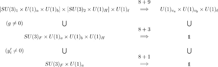
Figure 1: The symmetry breaking pattern of the model. Horizontal arrows represent the spontaneous symmetry breaking of Eq. 6. The numbers over each arrow count the number of NGB’s generated. The first row corresponds to the limit in which the gauge couplings and the small symmetry breaking operators of ${\cal L}_{Y}^{\prime}$ are set to zero, in which case $17$ NGB’s are produced. The vacuum symmetries $U(1)_{v_{a}}$ and $U(1)_{v_{b}}$ are shown in Eq. V.1. In the second row, the $SU(3)_{F}$ gauge coupling is turned on, and as a result only the diagonal combination of $SU(3)_{1}\times SU(3)_{2}$ is preserved in the EFT. At the same time, $SU(3)_{F}$ anomalies explicitly break lepton number $U(1)_{\ell}$. There are 11 NGB’s, and 6 PNGB’s with masses $\sim g^{2}F/4\pi$. In the third row, the operators in ${\cal L}_{Y}^{\prime}$ are turned on, explicitly breaking $U(1)_{b}$ (by $y_{u}^{\prime}$ and $y_{e}^{\prime}$) and $U(1)_{H}$ (by $y_{\nu}^{\prime}$). This gives mass to two of the 11 NGB’s. Of these, 8 disappear through the Higgs mechanism, and one is the candidate axion. Five additional global $U(1)$’s are explicitly broken by ${\cal L}_{Y}$, $U(1)_{B}$ is unbroken, and $U(1)_{Y}$ is broken spontaneously at the much lower electroweak scale $v$. They are not included here.

We next include the family gauge coupling and the small operators of ${\cal L}_{Y}^{\prime}$. As described above, the family gauge interaction makes anomalous one visible-sector $U(1)$, taken to be $U(1)_{\ell}$. Since the family gauge interaction and the third operator of ${\cal L}_{Y}^{\prime}$ explicitly break $SU(3)_{1}\times SU(3)_{2}\rightarrow SU(3)_{F}$, since the third operator of ${\cal L}_{Y}^{\prime}$ explicitly breaks $U(1)_{H}$, and since the first two break $U(1)_{b}$, the full symmetry of the EFT, excluding the SM interactions, is $SU(3)_{F}\times U(1)_{a}$, along with $U(1)_{B}$ and $U(1)_{Y}$. With the visible and hidden sectors now coupled by the family-gauge and ${\cal L}_{Y}^{\prime}$ interactions, the spontaneous breaking of the $SU(3)_{F}\times U(1)_{a}$ symmetry is complete, producing $9$ NGB’s, of which $8$ are eaten. The remaining NGB is the candidate axion. This count is described in the last line of Fig. 1.

Of the original $17$ NGB’s, therefore, $8$ have become PNGB’s. We discuss their masses by first noting that if only the family gauge interaction is included (second line of Fig. 1), $2$ of the PNGB’s, corresponding to the spontaneous breaking of $U(1)_{b}$ and $U(1)_{H}$, remain massless. The other $6$ develop masses at one-loop in the family gauge interaction, of order $g^{2}F/4\pi$.

There remain two PNGB’s associated with the explicit breaking of $U(1)_{b}$ and $U(1)_{H}$ by the operators of ${\cal L}_{Y}^{\prime}$. In the case of $U(1)_{H}$, a combination of $U(1)_{H}$ and $U(1)_{\ell}$ is still preserved by the operators of ${\cal L}_{Y}^{\prime}$ (and ${\cal L}_{Y}$). However, this ($SU(3)_{F}$-anomalous) symmetry is not an essential ingredient in the quark and charged-lepton phenomenology, and may be broken by additional operators which preserve $U(1)_{a}$, but are small enough not to disturb significantly the neutrino phenomenology of Ref. APY3 . We take these operators to be present generically. The explicit breaking of $U(1)_{b}$ by the first two operators of ${\cal L}_{Y}^{\prime}$ must be accompanied by a coupling (the family gauge coupling) between the visible and hidden sectors in order to make massive the associated NGB.

Consider now the bilinear part of the effective lagrangian involving the (P)NGB’s associated with the spontaneous breaking of $U(1)_{a}\times U(1)_{b}\times U(1)_{H}$. After proper diagonalization and normalization of the kinetic part, and neglecting QCD anomalies, there will exist a rank-two mass matrix generated at the multi-loop level. Its entries are proportional to $F^{2}$ with coefficients determined by the small parameters in ${\cal L}_{Y}^{\prime}$ and the family gauge coupling $g$. The $2$ resulting PNGB’s (as well as the $6$ PNGB’s with masses of order $g^{2}F/4\pi$) have non-diagonal couplings to the SM fermions (they are familons), while the massless NGB has diagonal couplings. In addition, since they all couple through the third operator of ${\cal L}_{Y}^{\prime}$ to the Majorana mass matrix of the neutrinos; they are Majorons. Clearly, $F$ must be taken large enough so that the $8$ PNGB’s lie beyond current experimental reach.

The weak coupling of the visible and hidden sectors by the family gauge interaction and the third interaction of ${\cal L}_{Y}^{\prime}$ means that $\langle H\rangle$ cannot in general be diagonalized in the frame in which $\langle S\rangle$ and $\langle\Sigma\rangle$ are diagonal. Its orientation, described by $3$ mixing angles, is a dynamical, vacuum alignment question. The mixing angles enter the neutrino mass matrix directly through the third operator of ${\cal L}_{Y}^{\prime}$ and they enter the quark and charged-lepton mass matrices through the $SU(3)_{F}$ radiative corrections since the gauge-boson mass matrix depends on $\langle H\rangle$.

The effective potential determining this orientation is generated from the weak couplings of the EFT as well as other possible weak interactions linking the two sectors in the underlying theory. To account for the CKM and Pontecorvo-Maki-Nakagawa-Sakata (PMNS) mixing angles, all the off-diagonal entries of $\langle H\rangle$ must be non-zero in the basis in which $\langle S\rangle$ and $\langle\Sigma\rangle$ are diagonal. Equivalently, the breaking pattern must not leave any residual $Z_{2}$ symmetries. (The local operators corresponding to the masses of the PNGB’s described above are a part of the full effective potential.)

Finally, we note that CP-violating phases are naturally present in the model. They can emerge from the underlying theory and are then present directly in the Yukawa couplings of the EFT. It can be seen that they cannot in general be removed from all allowed operators by phase rotations of the fields. Phases can also arise spontaneously through the weak effective potential coupling the visible and hidden sectors. The combination of all these phases will determine the measured CP-violating phase in the CKM matrix, and the predicted Dirac and Majorana phases in the leptonic (PMNS) matrix. If the spontaneously generated phases and those present in the operators of the EFT are $O(1)$, the same will be true of the measured and predicted phases.

V Yukawa Operators and Fermion Mass Matrices

In this section we examine the phenomenological effects of all admissible Yukawa operators, including those not in ${\cal L}_{Y}$ and ${\cal L}_{Y}^{\prime}$, making use of the EFT symmetries and the vacuum symmetries. We show that other allowed operators with the $U(1)_{a}\times U(1)_{b}$ symmetry of ${\cal L}_{Y}$ (or which break $U(1)_{b}$ by small amounts as in ${\cal L}_{Y}^{\prime}$), give no qualitatively new contributions to the mass matrices at zeroth order in the family gauge interaction.

The effect of the additional admissible operators we did not include is therefore at most a redefinition of some of the couplings that seed the mass matrices, and hence, even at loop-order in the family gauge interactions, leave the phenomenological success of ${\cal L}_{Y}$ and ${\cal L}_{Y}^{\prime}$ undisturbed.

V.1 Dominant Yukawa Operators

We first discuss Yukawa operators respecting the symmetries of ${\cal L}_{Y}$: $U(1)_{a}\times U(1)_{b}\times SU(3)_{1}$. The family gauge interaction is initially neglected, it’s effects to be included perturbatively. The operators of interest are bilinear in the fermion fields and include up to one power of the Higgs-doublet field $h$. Any number of $S$ and $\Sigma$ fields may be included since they are subject to the nonlinear constraints that freeze out all but NGB and PNGB degrees of freedom.

We begin with operators with $S$’s and $\Sigma$’s sandwiched between $q{\tilde{h}}$ and $u^{c}$, that is, operators potentially capable of directly giving up-type quark masses when the scalars develop VEV’s. If attention is restricted to operators with only one power of $S$ or $\Sigma$, as in ${\cal L}_{Y}$, there is no such quantity. But it easy to write down operators of this type if more powers of $S$ and $\Sigma$ are admitted. A simple example is $q{\tilde{h}}(S\times S)\times\Sigma^{*}u^{c}/\ F^{3}$, where $S\times S$ represents the $\bf 6$ in the product of the two $\bf\bar{6}$’s. Clearly this operator vanishes in the vacuum of Eq. 6, but what about the general class of such operators?

To answer this question, we note that under the $U(1)_{v_{a}}\times U(1)_{v_{b}}$ vacuum symmetry of the visible sector (Fig. 1), the fields transform as

$$q \rightarrow diag\{e^{i\theta_{a}},e^{-\frac{1}{2}i\theta_{a}+2i\theta_{b}},e^{-\frac{1}{2}i\theta_{a}+i\theta_{b}}\}\,q$$

$$u^{c} \rightarrow diag\{e^{i\theta_{a}-i\theta_{b}},e^{-\frac{1}{2}i\theta_{a}+i\theta_{b}},e^{-\frac{1}{2}i\theta_{a}}\}\,u^{c}$$

$$d^{c} \rightarrow diag\{e^{3i\theta_{a}-i\theta_{b}},e^{\frac{3}{2}i\theta_{a}+i\theta_{b}},e^{\frac{3}{2}i\theta_{a}}\}\,d^{c}$$

$$\chi \rightarrow diag\{e^{2i\theta_{a}-i\theta_{b}},e^{\frac{1}{2}i\theta_{a}+i\theta_{b}},e^{\frac{1}{2}i\theta_{a}}\}\,\chi$$

$$\chi^{c} \rightarrow diag\{e^{i\theta_{a}-3i\theta_{b}},e^{-\frac{1}{2}i\theta_{a}-i\theta_{b}},e^{-\frac{1}{2}i\theta_{a}-2i\theta_{b}}\}\,\chi^{c}$$

$$\ell \rightarrow diag\{e^{-10i\theta_{a}-2i\theta_{b}},e^{-\frac{23}{2}i\theta_{a}},e^{-\frac{23}{2}i\theta_{a}-i\theta_{b}}\}\,\ell$$

$$e^{c} \rightarrow diag\{e^{14i\theta_{a}+i\theta_{b}},e^{\frac{25}{2}i\theta_{a}+3i\theta_{b}},e^{\frac{25}{2}i\theta_{a}+2i\theta_{b}}\}\,e^{c}$$

$$h \rightarrow e^{-i\theta_{a}-i\theta_{b}}\,h$$

$$S \rightarrow diag\{e^{-\frac{3}{2}i\theta_{a}+i\theta_{b}},e^{-i\theta_{b}},1\}\,S\,diag\{e^{-\frac{3}{2}i\theta_{a}+i\theta_{b}},e^{-i\theta_{b}},1\}$$

$$\Sigma \rightarrow diag\{e^{-\frac{3}{2}i\theta_{a}+2i\theta_{b}},1,e^{i\theta_{b}}\}\,\Sigma\,diag\{e^{-\frac{3}{2}i\theta_{a}+2i\theta_{b}},1,e^{i\theta_{b}}\},$$

where $\theta_{a}$ and $\theta_{b}$ are the arbitrary parameters associated with the symmetries $U(1)_{a}$ and $U(1)_{b}$.

The most general mass operator involving $q$ and $u^{c}$, emerging from the VEV’s of $S$ and $\Sigma$, is of the form $q\tilde{h}\,diag\{y_{u_{1}},y_{u_{2}},y_{u_{3}}\}u^{c}$. In order that it be invariant under $U(1)_{v_{a}}\times U(1)_{v_{b}}$, we must have

$$diag\{y_{u_{1}},y_{u_{2}},y_{u_{3}}\} = diag\{e^{3i\theta_{a}},e^{4i\theta_{b}},e^{2i\theta_{b}}\}$$ (16)

$$\times diag\{y_{u_{1}},y_{u_{2}},y_{u_{3}}\}.$$

The only solution is $y_{u_{1}}=y_{u_{2}}=y_{u_{3}}=0$. Thus there is no Yukawa operator involving $q$ and $u^{c}$ giving a non-vanishing mass matrix.

One can show more generally that the mass matrices generated by the operators of ${\cal L}_{Y}$ are the most general fermion mass matrices allowed by $U(1)_{v_{a}}\times U(1)_{v_{b}}$. Consider, for example, a down-type operator with VEV’s of $S$ and $\Sigma$ sandwiched between $qh$ and $d^{c}$. It must be of the form $qh\,diag\{y_{d_{1}},y_{d_{2}},y_{d_{3}}\}d^{c}$. In order that it be invariant, we must have

$$diag\{y_{d_{1}},y_{d_{2}},y_{d_{3}}\} = diag\{e^{3i\theta_{a}-2i\theta_{b}},e^{2i\theta_{b}},1\}$$ (17)

$$\times diag\{y_{d_{1}},y_{d_{2}},y_{d_{3}}\},$$

Thus the only possible non-vanishing entry is the $33$ element, which is generated by the operator $y_{d}qhSd^{c}/F$ of ${\cal L}_{Y}$. Other operators may be written down that do the same thing, for example $qh(S\times\Sigma)\times\Sigma^{*}d^{c}/\ F^{3}$ with its own (complex) coefficient. It, too, has only a $33$ entry in the vacuum of Eq. 6.

A similar argument applies to all Yukawa operators respecting the symmetry $U(1)_{a}\times U(1)_{b}\times SU(3)_{1}$ of the visible sector. All operators that have non-vanishing VEV’s in the vacuum of Eq. 6, with it’s symmetry (Eq. V.1), give rise to the same mass matrices as those arising from the operators of ${\cal L}_{Y}$. For the charged-lepton sector there is only a $33$ entry. For the up-type sector, the entries lay the groundwork for the see-saw explanation of the masses.

To summarize, we have included in ${\cal L}_{Y}$ a minimal set of Yukawa operators necessary to explain, along with the $SU(3)_{F}$ gauge interaction, most features of the quark and charged-lepton mass matrices. The two $U(1)$ vacuum symmetries imply that the quark and charged-lepton mass matrices generated by the operators of ${\cal L}_{Y}$ are completely general. Perturbation theory in the family gauge interaction then couples the visible and hidden sectors, communicating the breaking of the two $U(1)$ vacuum symmetries to the visible sector, and leading to non-vanishing values for up-type and down-type quark mass ratios, CKM mixing angles, and charged-lepton mass ratios. They are finite and calculable within the EFT.

V.2 Smaller, Symmetry-Violating Yukawa Operators

To incorporate necessary small corrections to the quark- and charged-lepton mass matrices, and to generate the entire, small mass matrix of the neutrinos, the additional small operators of ${\cal L}_{Y}^{\prime}$, are required. The couplings $y_{e}^{\prime}$ and $y_{u}^{\prime}$ are $O(10^{-4})$, and $y_{\nu}^{\prime}$ is no larger than this if $F$ is no larger than about $10^{11}$ GeV. These operators together break $U(1)_{b}$, $U(1)_{H}$, and $SU(3)_{1}\times SU(3)_{2}\rightarrow SU(3)_{F}$, leaving the global $U(1)_{a}$ symmetry.

With $U(1)_{a}$ as the only global $U(1)$ symmetry, many other Yukawa operators, comparably small compared to those of ${\cal L}_{Y}^{\prime}$ and breaking $U(1)_{b}$, are allowed. Note that there is no distinction between $S$ and $\Sigma$ at this level since they have the same $U(1)_{a}$ charges. The question is whether any of these operators can give rise in the vacuum of Eq. 6 to fermion mass matrices that disturb the successful phenomenology based on the operators of ${\cal L}_{Y}^{\prime}$.

To see that this does not happen, note that the residual symmetry of the vacuum (present before gauge interactions link the visible and hidden sectors), with $U(1)_{b}$ now explicitly broken, is just $U(1)_{v_{a}}$. It can be read off from Eq. V.1 by setting $\theta_{b}=0$. This single $U(1)$ vacuum symmetry allows nonzero values for only the $22$ and $33$ entries of both $\langle S\rangle$ and $\langle\Sigma\rangle$. In the absence of the family gauge interaction, there can therefore be no masses present for the first-family quarks and charged leptons. This is an essential role of the $U(1)_{a}$ symmetry. Its spontaneous breaking in the hidden sector and transmittal to the visible sector by the family gauge interaction then produces the small, first-family masses.

The contributions arising from ${\cal L}_{Y}^{\prime}$ to the $22$ and $33$ entries of the quark and charged-lepton mass matrices are $O(10^{-4})$. They produce small but important corrections in the quark and lepton phenomenology  APY3 .

VI $U(1)_{a}$ and the QCD Axion

We have shown that a minimal EFT, capable of accounting for the quark and lepton masses, mixing angles, and phases  APY2  APY3 , naturally includes one global $U(1)$ symmetry, $U(1)_{a}$ of Table 2. The breaking pattern leaves an associated vacuum symmetry $U(1)_{v_{a}}$ (Eq. V.1) in the visible sector, protecting the first-family quarks and charged leptons from gaining mass in the absence of the $SU(3)_{F}$ family gauge interaction. The breaking of $U(1)_{v_{a}}$ in the hidden sector at scale $F$, communicated to the quarks and leptons by the $SU(3)_{F}$ gauge interaction, leads to finite first-family masses, and produces a so-far massless NGB.

Suppose next that the $U(1)_{a}$ symmetry is classically exact, respected by all operators of the EFT. Then, since it is anomalous due to QCD interactions, the NGB is a candidate for a QCD axion BK . The axion field is a linear combination of NGB fields in $S$, $\Sigma$, and $H$, the combination that remains massless and survives below the scales where the family gauge bosons and the PNGB’s decouple. (This is also below the scale where the $\chi$ and $\chi^{c}$ fields have been integrated out, having generated the up-type quark masses.) The linear combination is dictated by ratios of the dimensionless parameters that appear in the VEV’s of Eq. 6.

The axion couples to visible matter through the operators of ${\cal L}_{Y}$ and ${\cal L}_{Y}^{\prime}$. With the family gauge corrections included, these operators lead to the observed masses of all the quarks and leptons. Thus, in the effective theory at scales low enough so that only the SM fields and the axion survive, the axion couples to all the quarks and leptons with coupling strength given by $m_{f}/F_{a}$, where $m_{f}$ is the fermion mass and $F_{a}$ is related to $F$ by ratios the dimensionless parameters that appear in the VEV’s of Eq. 6. Since they are all expected to be roughly of the same order, $F_{a}$ is of the same order as $F$. Since the axion couples to neutrino mass through the Majorana operator in ${\cal L}_{Y}^{\prime}$, it is also a Majoron.

It is not our purpose to discuss the phenomenology of this axion candidate here, except to observe that with $F$ in the allowed window $10^{9}\lesssim F\lesssim 10^{12}$ GeV pdg ; kim , corresponding to a mass range $10^{-3}\gtrsim m_{a}\gtrsim 10^{-6}$ eV, it evades all axion and Majoron searches to date.

The $U(1)_{a}$ symmetry is a natural feature of the EFT operators required to compute quark and lepton mass matrices, and if taken to be exact it leads to a viable QCD axion. But the imbedding of this EFT in a larger framework could in general lead to higher-dimension operators that explicitly break $U(1)_{a}$ and give contributions to the axion potential that swamp the QCD contribution dine .

VII Summary

We have explored an effective field theory (EFT) framework proposed recently for the generation of quark and lepton mass matrices  APY2  APY3 . An $SU(3)$ family gauge symmetry, broken spontaneously at a high scale $F$, communicates symmetry breaking from a hidden sector to the visible-sector standard model fields.

To classify the Yukawa operators that seed the mass matrices, we have employed the set of global $U(1)$ symmetries that are naturally part of the EFT. The dominant required operators preserve two such symmetries, $U(1)_{a}$ and $U(1)_{b}$, in addition to baryon number and electroweak hypercharge. A set of smaller operators, necessary to generate the neutrino mass matrix and to provide small corrections to the quark and charged lepton mass matrices, preserve only $U(1)_{a}$ along with baryon number and electroweak hypercharge.

We have described the vacuum structure of the EFT, enumerating the Nambu-Goldstone bosons (NGB’s) and pseudo-Nambu Goldstone bosons (PNGB’s), as determined by the symmetry-breaking interactions that link the visible and hidden sectors. The PNGB’s that gain mass because of the family gauge coupling and the small symmetry-breaking Yukawa operators, couple off-diagonally in family space (they are familons), and couple to the Majorana mass matrix of the neutrinos (they are Majorons).

We have used the vacuum structure together with the symmetries of the EFT to classify the quark and charged-lepton masses that emerge. CP-violating phases, which lead to the CKM phase as well as Dirac and Majorana phases in the leptonic PMNS matrix, arise spontaneously within the EFT, and also enter the parameters of the EFT directly from the underlying physics.

The $U(1)_{a}$ symmetry is unbroken by any of the phenomenologically necessary interactions of the EFT, except for QCD anomalies. The spontaneous breaking pattern preserves an associated vacuum symmetry, $U(1)_{v_{a}}$, in the visible sector, enforcing the masslessness of the first-family quarks and charged leptons in the absence of the family gauge interaction. The $U(1)_{v_{a}}$ symmetry is broken in the hidden sector at the family-breaking scale $F$, with the breaking communicated to the standard-model fields by the family gauge interaction.

If the $U(1)_{a}$ symmetry is taken to be exact in the EFT except for QCD anomalies (a Peccei-Quinn symmetry), and if $F$ is taken to lie in the allowed window $10^{9}<F<10^{12}$ GeV, then the associated PNGB is a viable axion, coupling to all the particles of the standard model. This conclusion relies on the large hierarchy between $F$ and the electroweak scale $v$. Also, it is not clear whether the $U(1)_{a}$ symmetry survives the imbedding of the EFT in a larger framework.

VIII Appendix - Nonlinear Constraints

We summarize here the nonlinear constraints that must emerge from the underlying dynamics in the visible sector and the hidden sector, corresponding to the VEV pattern of Eq. 6 and reducing the degree-of-freedom count to only the NGB’s. The nonlinear constraints for $S$ are

$${\rm Tr}[SS^{*}] = s^{2}F^{2}$$ (18)

$${\rm Tr}[(S\times S)(S\times S)^{*}] = 0.$$ (19)

With $S$ written in the form

$$S=\left(\begin{array}[]{ccc}s_{11}&s_{12}&s_{13}\\ s_{12}&s_{22}&s_{23}\\ s_{13}&s_{23}&s_{33}\\ \end{array}\right),$$ (20)

where the the $s_{ij}$ are complex fields, Eq. 18 gives one constraint for these 12 real fields.

Eq. 19 can be written in the form

$${\rm Tr}[(S\times S)(S\times S)^{*}]$$ (21)

$$= |s_{11}s_{22}-s^{2}_{12}|^{2}+|s_{11}s_{33}-s^{2}_{13}|^{2}+|s_{22}s_{33}-s^{2}_{23}|^{2}$$

$$+2|s_{12}s_{13}-s_{11}s_{23}|^{2}+2|s_{12}s_{23}-s_{22}s_{13}|^{2}$$

$$+2|s_{13}s_{23}-s_{33}s_{12}|^{2}$$

$$= 0.$$

Each of the absolute values must vanish, leading to a set of three, independent complex equations ($6$ constraints in all) . They can be taken to be

$$s_{11}s_{22}=s^{2}_{12}$$ (22)

$$s_{11}s_{33}=s^{2}_{13}$$ (23)

$$s_{22}s_{33}=s^{2}_{23}$$ (24)

The same constraints apply to the elements of $\Sigma$.

The nonlinear constraint coupling $S$ and $\Sigma$ is:

$${\rm Tr}[S\Sigma^{*}S^{*}\Sigma]=0\,.$$

It can be written in the form

$$|s_{12}\sigma_{12}s_{23}\sigma_{23}+s_{12}\sigma_{12}s_{13}\sigma_{13}+s_{23}\sigma_{23}s_{13}\sigma_{13}|^{2}$$ (25)

$$\times|s_{12}\sigma^{*}_{12}s_{23}\sigma^{*}_{23}+s_{12}\sigma^{*}_{12}s_{13}\sigma^{*}_{13}+s_{23}\sigma^{*}_{23}s_{13}\sigma^{*}_{13}|^{2}$$

$$/|s_{12}s_{13}s_{23}\sigma_{12}\sigma_{13}\sigma_{23}|^{2}$$

$$= 0\,,$$

where $\sigma_{ij}$ are the elements of $\Sigma$. This form, which is a set of $2$ constraints, is written making use of the separate nonlinear constraints on $S$ and $\Sigma$. Thus the total number of constraints is $16$, reducing the $24$ degrees of freedom in $S$ and $\Sigma$ to the $8$ NGB’s of the visible sector.

These constraints also lead to the VEV’s of Eq. 6. If we rotate $\langle S\rangle$ into diagonal form, then the nonlinear constraints on $S$ allow only one non-vanishing element which we take to be the $33$ element. The constraint coupling $S$ and $\Sigma$ then gives $\langle\sigma_{33}\rangle=0$. But then the above constraint equations on $S$, with $s_{ij}$ replaced by $\sigma_{ij}$, demand that $\langle\sigma_{13}\rangle=\langle\sigma_{23}\rangle=0$. Then $\langle\Sigma\rangle$ can be put into diagonal form by an $SU(2)$ transformation leaving $\langle S\rangle$ untouched. The constraints on $\Sigma$ demand that only one element be nonzero, which we take to be the $22$ element.

We note that each of the above constraints can be derived from an appropriate potential providing a phenomenological description of the underlying dynamics LFLi . We assume here that they emerge from the true underlying theory, the UV completion of our EFT.

In a similar manner, the set of $3$ nonlinear constraints on the hidden-sector $H$ is

$${\rm Tr}[HH^{*}] = O(1)\,F^{2}$$

$${\rm Tr}[(H\times H)(H\times H)^{*}] = O(1)\,F^{4}$$

$$|{\rm det}\,H| = O(b^{2})\,F^{3},$$ (26)

reducing the $12$ degrees of freedom in $H$ to the $9$ NGB’s of the hidden sector. There are now a total of $17$ NGB’s Once the visible and hidden sectors are linked by the family gauge interaction and the third operator of ${\cal L}_{Y}^{\prime}$, all but $9$ of these become PNGB’s.

- (1) T. Appelquist, Y. Bai and M. Piai, Phys. Lett. B 637, 245 (2006) [arXiv:hep-ph/0603104].
- (2) T. Appelquist, Y. Bai and M. Piai, Phys. Rev. D 74, 076001 (2006) [arXiv:hep-ph/0607174].
- (3) R. D. Peccei and H. R. Quinn, Phys. Rev. Lett. 38, 1440 (1977).
- (4) F. Wilczek, Phys. Rev. Lett. 40, 279 (1978); S. Weinberg, Phys. Rev. Lett. 40, 223 (1978).
- (5) J. Wess and B. Zumino, Phys. Lett. B 37, 95 (1971); E. Witten, Nucl. Phys. B 223, 422 (1983);
- (6) The possible existence of a Peccei-Quinn symmetry and associated axion in the context of models with an family symmetry was noted by Z.G.Berezhiani and M.Yu.Khlopov, Yadernaya Fizika (1990) V. 51, PP. 1157-1170. [English translation: Sov.J.Nucl.Phys. (1990) V. 51, PP. 739-746]; Z.Phys.C- Particles and Fields (1991), V. 49, PP. 73-78.
- (7) W. M. Yao et al. [Particle Data Group], J. Phys. G 33, 1 (2006).
- (8) P. Sikivie, hep-ph/0509198, J. E. Kim, hep-ph/0612141
- (9) M. Dine, arXiv:hep-ph/0011376.
- (10) For the analysis of a potential with a single sextet field, see: L. F. Li, Phys. Rev. D 9, 1723 (1974).