MZ-TH/06-27

QCD condensates
of dimension $D=6$ and $D=8$
from hadronic $\tau$-decays

Abstract

The high-precision data from hadronic $\tau$ decays allows one to extract information on QCD condensates. Using the finalized ALEPH data, we obtain a more rigorous determination of the dimension 6 and 8 condensates for the $V-A$ correlator. In particular, we find that the recent data fix a certain linear combination of these QCD condensates to a precision at the level of $O(2)\,\%$. Our approach relies on more general assumptions than alternative approaches based on finite energy sum rules.

1 Introduction

The physics of hadronic $\tau$ decays has been an important testing ground for QCD since long. The precise data from the LEP collaborations have allowed us to obtain invaluable information on fundamental and effective parameters of the theory. With the completion of the final analysis by the ALEPH collaboration [1] it is timely to exploit these data also for a more precise extraction of QCD condensate parameters.

In a previous letter [2] we had used earlier ALEPH data [3] in a functional method to extract within rather general assumptions the QCD condensate of dimension $D=6$ related to the $V-A$ current. Here we report the results of a reanalysis using the more precise final data from ALEPH. Moreover, we found that the higher quality of the experimental data allows us also to obtain information on the condensates of higher dimension. In particular, we find that the data imply a strong correlation between $D=6$ and $D=8$ $V-A$ condensates.

We extract the condensates from a comparison of the time-like experimental data with the asymptotic space-like results from theory. The assumptions of our approach are quite general. The essential property of the exact correlator in the space-like region on which our approach relies is that its fall-off with the 4-momentum squared $s$ is determined by at most two lowest-dimension terms in the operator product expansion (OPE). When we aim at a determination of the $D=6$ condensate, we assume a fall-off like $1/s^{3}$ within an error band that scales like $1/s^{4}$. In the analysis where we want to determine the $D=6$ and $D=8$ condensates, we correspondingly assume a fall-off like a sum of $1/s^{3}$ and $1/s^{4}$ terms within an error band described by a $1/s^{5}$ term. These assumptions are more general than those of other approaches since they do not refer to the positive axis in the $s$-plane. Furthermore our assumptions are quite independent of perturbation theory or indeed of QCD itself. Similarly to the Weinberg sum rules, they only depend on the pattern of chiral symmetry breaking. Of course, as QCD is well established, we like to discuss our results in the language of QCD and the OPE. For this reason we also include the $O(\alpha_{s})$ correction to the $1/s^{3}$ term. If it was available, we could have included the perturbative correction to the $1/s^{4}$ term as well. However, as we will see, the inclusion of higher-order terms does not qualitatively affect our results.

One should, however, keep in mind that it is not possible (not even in principle) to reconstruct the correlator in the space-like region from error afflicted time-like data, as this constitutes an analytic continuation from a finite domain. One has to stabilize this “ill-posed problem” by suitable additional assumptions. For example, the application of finite energy sum rules (FESR) for an extraction of QCD condensates could be justified if the result of QCD and the operator product expansion in the space-like region is simply a series in powers of $1/s$ times condensates (vacuum expectation values of operators) and if there are no truly non-perturbative terms. In this case, each moment would pick out a single operator. However, this is unfortunately not the case since logarithms arising within perturbation theory do not fall in this class of functions. The higher and lower dimensional condensates contribute to a given moment starting with the inclusion of corrections of order $O(\alpha_{s}^{2})$ [4]. It is also known that the perturbation series starts to diverge at some, not very high, order. As higher orders of the relevant Wilson coefficients are not known, one can only hope that the extraction of the condensates is stable when correction terms are included. There is the additional problem of the contribution of the truly non-perturbative terms (non-OPE) to the integral on the circle in the complex plane, even if this uncertainty, which is expected to be most prominent near the physical cut, can be reduced by choosing suitable linear combinations of moments.

We should expect that there is a price to be paid for the generality of assumptions of our approach. However, even if it turns out that the errors in the values of the extracted parameters are relatively large, we can hope that our results lend additional confidence to the numerical results obtained with the help of FESR.

2 QCD condensates

We consider the polarization operator of hadronic vector and axial-vector charged currents, $J_{\mu}=V_{\mu}=\bar{u}\gamma_{\mu}d$ and $J_{\mu}=A_{\mu}=\bar{u}\gamma_{\mu}\gamma_{5}d$,

$$\Pi_{\mu\nu}^{J} = i\int dxe^{iqx}\langle TJ_{\mu}(x)J_{\nu}(0)^{\dagger}\rangle$$

$$= \left(-g_{\mu\nu}q^{2}+q_{\mu}q_{\nu}\right)\Pi_{J}^{(0+1)}(q^{2})+g_{\mu\nu}q^{2}\Pi_{J}^{(0)}(q^{2})\,.$$

The conservation of the vector current implies $\Pi_{V}^{(0)}=0$. The connection to experimental observables is most easily expressed with the help of the spectral functions which are related to the absorptive part of the correlators. Keeping the normalization as defined in most of the experimental publications, the functions

$$v_{j}(s)=2\pi{\rm Im}\Pi_{V}^{(j)}(s),~{}~{}~{}~{}a_{j}(s)=2\pi{\rm Im}\Pi_{A}^{(j)}(s)$$ (2)

can be extracted from the decay spectrum of hadronic $\tau$-decays. We restrict the present study to the $V-A$ component which is related to the branching ratios of $\tau$ decays,

$$R_{\tau,{\rm V-A}}=\frac{B(\tau\rightarrow\nu_{\tau}+{\rm hadrons},~{}{\rm V-A})}{B(\tau\rightarrow\nu_{\tau}+e+\bar{\nu}_{\tau})}\,,$$ (3)

through

$$v_{1}(s)-a_{1}(s) = \frac{m_{\tau}^{2}}{6\left|V_{ud}\right|^{2}S_{{\rm EW}}}\frac{{\rm d}R_{\rm V-A}}{{\cal B}_{e}{\rm d}s}\left(1-\frac{s}{m_{\tau}^{2}}\right)^{-2}\left(1+2\frac{s}{m_{\tau}^{2}}\right)^{-1}\,,$$ (4)

$$a_{0}(s) = \frac{m_{\tau}^{2}}{6\left|V_{ud}\right|^{2}S_{{\rm EW}}}\frac{{\rm d}R_{\rm A}}{{\cal B}_{e}{\rm d}s}\left(1-\frac{s}{m_{\tau}^{2}}\right)^{-2}\,.$$ (5)

Here, ${\cal B}_{e}=0.17810\pm 0.00039$ [1] is the branching fraction of the electron channel, $V_{ud}$ is the CKM-matrix element, $\left|V_{ud}\right|=0.9746\pm 0.0006$ [5], the $\tau$ mass is $m_{\tau}=1.777$ GeV and $S_{\rm EW}=1.0198\pm 0.0006$ accounts for electroweak radiative corrections [6]. The spin-0 axial vector contribution $a_{0}(s)$ is dominated by the one-pion state, $a_{0,\pi}(s)=2\pi^{2}f_{\pi}^{2}\delta(s-m_{\pi}^{2})$, with the $\pi$-decay constant $f_{\pi}=0.1307$ GeV [7].

We use the final experimental data from the ALEPH collaboration [1] because they have the smallest experimental errors. They are given by binned and normalized event numbers related to the differential distribution $dR_{\tau,V,A}/ds$. The quality of these data has increased a lot as compared to those of Ref. [3] which we used in our previous analysis [2]: first, the higher statistics has allowed the ALEPH collaboration to double the number of bins, and, secondly, the experimental errors decreased due to both higher statistics and a better understanding of systematic errors.

The $(V-A)$ correlator is special since it vanishes identically in the chiral limit ($m_{q}=0)$ to all orders in QCD perturbation theory. Renormalon ambiguities are thus avoided. We will neglect in our analysis perturbative contributions proportional to the light quark masses. Non-perturbative terms can be calculated for large $\left|s\right|$ by making use of the operator product expansion of QCD

$$\Pi_{\rm V-A}^{(0+1)}(s)=\sum_{D\geq 6}\frac{{\cal O}_{D}^{\rm V-A}}{(-s)^{D/2}}\left(1+c_{D}^{\rm NLO}\frac{\alpha_{s}(\mu^{2})}{\pi}+O(\alpha_{s}^{2})\right)$$ (6)

where ${\cal O}_{D}^{\rm V-A}$ are vacuum matrix elements of local operators of dimension $D$. For the correlator with spin $0+1$ and in the chiral limit, the sum begins with terms of dimension $D=6$. Assuming vacuum dominance or the factorization approximation which holds, e.g., in the large-$N_{C}$ limit, the matrix elements can be written as

$${\cal O}_{6}^{\rm V-A} = -\frac{64\pi}{9}\alpha_{s}\langle\bar{q}q\rangle^{2}\,,~{}~{}~{}~{}~{}c_{6}^{\rm NLO}=\frac{1}{4}\left[\tilde{c}_{6}+\mbox{ln}\left(\frac{\mu^{2}}{-s}\right)\right]\,;$$

$${\cal O}_{8}^{\rm V-A} = -4\pi\alpha_{s}i\left(1-N_{C}^{-2}\right)\langle\bar{q}q\rangle\langle\bar{q}\gamma^{\alpha\beta}G_{\alpha\beta}q\rangle\,;$$ (7)

$${\cal O}_{10}^{\rm V-A} = -\frac{8}{9}\pi\alpha_{s}\langle\bar{q}q\rangle^{2}\left(\frac{50}{9}m_{0}^{4}+32\pi\alpha_{s}\langle G_{\alpha\beta}G^{\alpha\beta}\rangle\right)\,.$$

The complete expression for ${\cal O}_{6}^{\rm V-A}$ is known to involve two operators [10]. However, our analysis does not rely on the factorization hypothesis since we are going to determine ${\cal O}_{6}^{\rm V-A}$ and ${\cal O}_{8}^{\rm V-A}$, but not the condensates $\langle\bar{q}q\rangle$ or $\langle\bar{q}\gamma_{\alpha\beta}G^{\alpha\beta}q\rangle$ separately. In the result for ${\cal O}_{10}^{\rm V-A}$ [11], $m_{0}^{2}$ is defined through the 5-dimensional quark-gluon mixed condensate. Starting from the second order, coefficients in perturbation theory depend on the regularisation scheme implying that the values of the condensates are scheme-dependent quantities. The NLO corrections for ${\cal O}_{6}^{\rm V-A}$ were computed first in [12] and the coefficient $\tilde{c}_{6}$ was found equal to $247/12$. This calculation was based on the BM definition of $\gamma_{5}$ in dimensional regularisation. A different treatment of $\gamma^{5}$ as used in Ref. [13] leads to $\tilde{c}_{6}=89/12$.

The typical scales determining the condensates are around 300 MeV. For example, from the Gell-Mann–Oakes–Renner relation [14] one has $\langle\bar{q}q\rangle\simeq-(250\,{\rm MeV})^{3}$, and from charmonium sum rules one expects ($\alpha_{s}/\pi)\langle G^{2}\rangle\simeq(300\,{\rm MeV})^{4}$ [15]. Taking the results from FESR approaches as a guide, we expect also ${\cal O}_{8}^{\rm V-A}$ and ${\cal O}_{10}^{\rm V-A}$ to be of order $10^{-3}$ GeV⁸ and $10^{-3}$ GeV¹⁰, resp. (see e.g. [16]). This is small enough so that the OPE makes sense. If ${\cal O}_{8,10}^{\rm V-A}$ would be much larger, radiative corrections to higher-dimension condensates would mix significantly with the lower-dimension ones through their imaginary parts.

In the following we shall summarize the functional method introduced in Ref. [2] which allows, in principle, to extract the condensates from a comparison of the data with the asymptotic space-like QCD results under rather general assumptions.

We consider a set of functions $F(s)$ (to be identified with $\Pi_{\rm V-A}^{(0+1)}(s)$) expressed in terms of some squared energy variable $s$ which are admissible as a representation of the true amplitude if

• $F(s)$ is a real analytic function in the complex $s$-plane cut along the time-like interval $\Gamma_{R}=[s_{0},\infty)$. The value of the threshold $s_{0}$ depends on the specific physical application ($s_{0}=(2m_{\pi})^{2}$ for $\Pi_{V}$, $s_{0}=m_{\pi}^{2}$ for $\Pi_{A}$).

• The asymptotic behavior of $F(s)$ is restricted by fixing the number of subtractions in the dispersion relation between $F(s)$ and its imaginary part along the cut $f(s)={\rm Im}F(s+i0)|_{s\in\Gamma_{R}}$ (for $\Pi_{\rm V-A}^{(0+1)}(s)$ no subtractions are needed):

  $$F(s)=\frac{1}{\pi}\int_{0}^{\infty}\frac{f(x)}{x-s}dx+\frac{f_{\pi}^{2}}{s}\,,$$ (8)

  where the term with $f_{\pi}^{2}$ accounts for the contribution from the pion pole, $a_{0}$ (Eq. 5), so that $f(x)$ can be taken directly from the ALEPH data.

We have two sources of information which will be used to determine $F(s)$ and $f(s)$. First, there are experimental data in a time-like interval $\Gamma_{\rm exp}=[s_{0},s_{\rm max}]$ with $s_{0}>0$ for the imaginary part of the amplitude. Although these data are given on a sequence of adjacent bins, we describe them by a function $f_{{\rm exp}}(s)$. We assert that $f_{{\rm exp}}$ is a real, not necessarily continuous function. The experimental precision of the data is described by a covariance matrix $V(s,s^{\prime})$.

On the other hand, we have a theoretical model, in fact QCD. From perturbative QCD we can obtain a prediction for the amplitude in a  space-like interval $\Gamma_{L}=[s_{2},s_{1}]$. This model amplitude is a continuous function of real type, but does not necessarily conform to the analyticity property i). Since perturbative QCD is expected to be reliable for large energies, we expect that there is also useful information about the imaginary part of the amplitude provided that $|s|$ is large, i.e. we can also use QCD predictions for $f(s)={\rm Im}F(s+i0)|_{s\in(s_{\rm max},\infty)}$. To implement this idea, we rewrite the dispersion relation (8) in the following way:

$$F(s)-\frac{f_{\pi}^{2}}{s}-\frac{1}{\pi}\int_{s_{\rm max}}^{\infty}\frac{f(x)}{x-s}dx=\frac{1}{\pi}\int_{0}^{s_{\rm max}}\frac{f(x)}{x-s}dx\,.$$ (9)

Then we can calculate the left-hand side of this equation in QCD,

$$\widetilde{F}_{\rm QCD}(s):=F_{\rm QCD}(s)-\frac{f_{\pi}^{2}}{s}-\frac{1}{\pi}\int_{s_{\rm max}}^{\infty}\frac{f_{\rm QCD}(x)}{x-s}dx\,,$$ (10)

whereas the right-hand side can be determined from experimental data. Thus we shall test the hypothesis whether the left-hand side of (9) can be described by QCD while the right-hand side describes the experimental data.

In order to do that, we need an a-priori estimate of the accuracy of the QCD predictions. This can be described by a continuous, strictly positive function $\sigma_{L}(s)$ for $s\in\Gamma_{L}$ which should encode errors due to the truncation of the perturbative series and the operator product expansion. It is expected to decrease as $|s|\rightarrow\infty$ and diverge for $s\rightarrow 0$. In Ref. [2] we aimed at a determination of the $D=6$ condensate of $\Pi_{\rm V-A}$. There we were allowed to consider the contribution of the dimension $D=8$ operator as an error, using $\sigma_{L}(s)=|{\cal O}^{\rm V-A}_{8}|_{\rm max}/s^{4}$ with $|{\cal O}^{\rm V-A}_{8}|_{\rm max}$ in the order of $10^{-3}\,{\rm GeV}^{8}$. If the perturbative part dominates, as is the case for the individual vector or axial vector correlators, the last known term of the perturbation series could be used as a sensible estimate of the error corridor, possibly combined with the first omitted term in the series over condensates. In the present work, we focus on obtaining information on the correlation of the condensates ${\cal O}^{\rm V-A}_{6}$ and ${\cal O}^{\rm V-A}_{8}$; therefore we will use in a similar way an estimate of $|{\cal O}^{\rm V-A}_{10}|_{\rm max}$ to define an error corridor which, in this case, scales with $1/s^{5}$.

The goal is to check whether there exists any function $F(s)$ with the above analyticity properties, the true amplitude, which is in accord with both the data in $\Gamma_{{\rm exp}}$ and the QCD model in $\Gamma_{L}$. In order to quantify the agreement we will define functionals $\chi_{L}^{2}[f]$ and $\chi_{R}^{2}[f]$ using an $L^{2}$ norm. For the time-like interval we simply compare the true amplitude $f(s)$ with the data and use the covariance matrix of the experimental data as a weight function:

$$\chi_{R}^{2}[f]=\frac{1}{|\Gamma_{\rm exp}|}\int_{s_{0}}^{s_{\rm max}}dx\int_{s_{0}}^{s_{\rm max}}dx^{\prime}\,V^{-1}(x,x^{\prime})\left(f(x)-f_{{\rm exp}}(x)\right)\left(f(x^{\prime})-f_{{\rm exp}}(x^{\prime})\right)\,.$$ (11)

Experimental data correspond to cross sections measured in bins of $s$, so that we can calculate this integral in terms of a sum over data points. The ALEPH data which we use are given for 140 equal-sized bins of width $\Delta s=0.025$ GeV² between $0$ and $3.5$ GeV². $\chi_{R}^{2}$ given in (11) is in fact the conventional definition of a $\chi^{2}$ normalized to the number of degrees of freedom and has a probabilistic interpretation: for uncorrelated data obeying a Gaussian distribution we would expect to obtain $\chi_{R}^{2}=1$. Since experimental data at different energies are correlated, we instead expect

$$\chi_{{\rm exp}}^{2}=\frac{1}{N}\sum_{i,j}\sqrt{V(s_{i},s_{i})V(s_{j},s_{j})}V^{-1}(s_{i},s_{j})\,.$$ (12)

In order to define a measure for the agreement of the true function $f(s)$ with theory, we use the left-hand side of (9) which is well-defined and expected to be a reliable prediction of QCD in the space-like interval for not too small $|s|$. This expression can be compared with the corresponding integral over the true function. Thus we define

$$\chi^{2}_{L}[f]=\frac{1}{|\Gamma_{L}|}\int_{\Gamma_{L}}w_{L}(x)\left(\widetilde{F}_{{\rm QCD}}(x)-\frac{1}{\pi}\int_{s_{0}}^{s_{\rm max}}\frac{f(x^{\prime})}{x^{\prime}-x}dx^{\prime}\right)^{2}dx$$ (13)

where $w_{L}$ is the weight function for the space-like interval and identified with $1/\sigma_{L}^{2}(s)$.

In order to find a best estimate of the function $f(s)$, we minimize $\chi_{L}^{2}$ subject to the condition $\chi^{2}_{R}[f]\leq\chi^{2}_{\rm exp}$. The solution can be obtained by solving a Fredholm equation of the second kind. This can be done numerically by expanding $f(s)$ in terms of Legendre polynomials (see Ref. [2] for details). The algorithm to determine an acceptable value for the condensate is then the following:

• For the given value of $\chi^{2}_{\rm exp}$ we determine the solution for $f(s)$ iteratively and calculate the corresponding value of $\chi_{L}^{2}[f]$ as a function of ${\cal O}_{D}^{\rm V-A}$.

• We minimize this $\chi_{L}^{2}[f]$ with respect to the values of ${\cal O}_{D}^{\rm V-A}$.

• We determine the error on the condensates by solving $\chi_{L}^{2}=\chi_{L,{\rm min}}^{2}+\Delta\chi^{2}$, where $\Delta\chi^{2}$ is chosen in the conventional way to reflect 1 or 2$\sigma$ confidence regions for the values of ${\cal O}_{D}^{\rm V-A}$.

The size of $\sigma_{L}$ determines the minimal value of $\chi_{L}^{2}$ according to Eq. (13) that can be reached by this algorithm. Obviously, widening the error corridor (increasing $\sigma_{L}$) will lead to values for $\chi_{L,{\rm min}}^{2}$ as small as desired. In such a case, the information obtained from the fit is not conclusive, since any model function $f(s)$ can be made consistent with the data if one allows for a wide enough error corridor. On the other hand, narrowing the error corridor will increase $\chi_{L,{\rm min}}^{2}$, signalling a bad fit, i.e. bad consistency of theory with data if the model function is not perfectly describing the data. However, a non-trivial result of our approach is the fact, that there exists a choice for the error corridor that leads to values $\chi_{L,{\rm min}}^{2}=O(1)$. We shall assume that the underlying probability distribution is Gaussian, and choose $\chi_{L,{\rm min}}^{2}$ and accordingly $\sigma_{L}$ such that the fit result corresponds to a $1\sigma$ CL. In practice this is done by adjusting $|{\cal O}^{\rm V-A}_{8}|_{\rm max}$ (for the 1-parameter fit of ${\cal O}^{\rm V-A}_{6}$) or $|{\cal O}^{\rm V-A}_{10}|_{\rm max}$ (for the 2-parameter fit of ${\cal O}^{\rm V-A}_{6}$ and ${\cal O}^{\rm V-A}_{8}$).

3 Numerical results and discussion

We start with a discussion of results obtained by 1-parameter fits of the dimension $D=6$ condensate. We find a consistent description of the data by QCD predictions including a non-zero value of ${\cal O}^{\rm V-A}_{6}$ as in our previous publication. The quality of the fit is good, i.e. a value of $\chi_{L,{\rm min}}^{2}$ corresponding to a $1\sigma$ CL can be fixed by choosing an error corridor described by the contribution from an ${\cal O}^{\rm V-A}_{8}$ condensate of the expected size of $\simeq 1.3\cdot 10^{-3}$ GeV⁸. A direct comparison of the data with the regularised function $f(s)$ (see Fig. 1) shows a nice agreement over the full range of $s$ with the exception of the highest $s$-bins, where experimental errors are large. In comparison with [2], the agreement between data and theory has improved. A number of consistency checks, as described in [2], has been performed and did not reveal any problem.

Figure 1: The regularised function $f(s)$ compared with ALEPH data [1] (left). The right figure shows the difference.

The results of the 1-parameter fit can be summarized by quoting values for ${\cal O}_{6}^{\rm V-A}$ at LO and at NLO for the two available values of the NLO coefficients:

$${\cal O}_{6}^{\rm V-A} = -5.9^{+1.7}_{-1.0}\times 10^{-3}{\rm GeV}^{6}~{}~{}~{}{\rm for}~{}~{}~{}\tilde{c}_{6}=0,~{}~{}\mbox{LO}\,,$$ (14)

$${\cal O}_{6}^{\rm V-A} = -4.9^{+1.5}_{-1.1}\times 10^{-3}{\rm GeV}^{6}~{}~{}~{}{\rm for}~{}~{}~{}\tilde{c}_{6}=\frac{89}{12}\,,$$ (15)

$${\cal O}_{6}^{\rm V-A} = -3.6^{+1.2}_{-1.2}\times 10^{-3}{\rm GeV}^{6}~{}~{}~{}{\rm for}~{}~{}~{}\tilde{c}_{6}=\frac{247}{12}\,.$$ (16)

The NLO results are based on the 4-loop expression for $\alpha_{s}$ with $\Lambda_{\overline{{\rm MS}}}(N_{f}=3)=0.326$ GeV and the renormalization scale chosen equal to $|s|$. They are not sensitive to changing $\Lambda_{\overline{{\rm MS}}}$ within the present experimental error of $\pm 0.030$ GeV. Moreover, the fit results based on the two different values of the NLO coefficients $\tilde{c}_{6}$ agree within errors and their difference with respect to the LO result is consistent with a shift calculated from the correction term choosing a typical value of $O(1.5)$ GeV for the renormalization scale in $\alpha_{s}$. This is to be expected since our method would work for any $s$-dependent ansatz for ${\cal O}^{\rm V-A}_{6}$ as well.

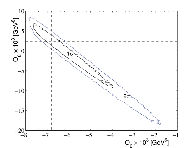
Figure 2: 1- and $2\sigma$ CL regions in the $({\cal O}_{6}^{\rm V-A},{\cal O}_{8}^{\rm V-A})$-plane from the 2-parameter fit (LO). The central values are marked by the dashed lines.

The main result of our present analysis is obtained from a 2-parameter fit of the dimension $D=6$ and $D=8$ condensates. Here we do not include the NLO contribution to ${\cal O}_{6}^{\rm V-A}$ since the corresponding NLO coefficient for ${\cal O}_{8}^{\rm V-A}$ is not known. In this case we find agreement of theory and data at the $1\sigma$ CL if we choose an error corridor described by the dimension $D=10$ contribution with the value $\simeq 5.7\cdot 10^{-3}$ GeV¹⁰. The result presented in Fig. 2 shows a strong negative correlation of ${\cal O}^{\rm V-A}_{6}$ and ${\cal O}^{\rm V-A}_{8}$. Both the central values as well as the errors from the 2-parameter fit are consistent with those from the LO 1-parameter analysis: The $1\sigma$ range allowed for ${\cal O}^{\rm V-A}_{6}$ for fixed ${\cal O}^{\rm V-A}_{8}=0$ (which is the assumption underlying the 1-parameter fit) agrees with (14). However, leaving the value of ${\cal O}^{\rm V-A}_{8}$ unconstrained, as in the 2-parameter fit, one finds a much larger range for ${\cal O}^{\rm V-A}_{6}$. The minimum value of $\chi_{L}^{2}$ for the 2-parameter fit is located at the values

$${\cal O}_{6}^{\rm V-A} = -6.8_{-0.8}^{+2.8}\times 10^{-3}\mbox{GeV}^{6}\,,$$

$${\cal O}_{8}^{\rm V-A} = 2.4_{-11.7}^{+4.5}\times 10^{-3}\mbox{GeV}^{8}\,.$$ (17)

The errors on ${\cal O}_{6}^{\rm V-A}$ for fixed ${\cal O}_{8}^{\rm V-A}$ are small, but the allowed range for ${\cal O}_{8}^{\rm V-A}$ is not very restrictive (note the different scales for the two condensates in Fig. 2). However, the strong correlation allows one to determine a linear combination of ${\cal O}_{6}^{\rm V-A}$ and ${\cal O}_{8}^{\rm V-A}$ with a rather small error:

$${\cal O}_{8}^{\rm V-A}+3.04~{}\mbox{GeV}^{2}\cdot{\cal O}_{6}^{\rm V-A}=-18.30^{-0.25}_{+0.38}\times 10^{-3}\mbox{GeV}^{8}\,.$$ (18)

We also checked that we obtain consistent results when including the NLO correction to ${\cal O}_{6}^{\rm V-A}$: The 1- and $2\sigma$ contours are shifted, essentially without changing their form, to larger values of ${\cal O}_{6}^{\rm V-A}$ exactly as can be inferred from the 1-parameter fits: for $\tilde{c}_{6}=0$ ($89/12,247/12$) we find the minimum of $\chi_{L}^{2}$ at ${\cal O}_{6}^{\rm V-A}\times 10^{3}/\mbox{GeV}^{6}=-6.8~{}(-6.6,-5.8)$.

There exist a number of previous extractions of QCD condensates in the literature, all based on a sum rule approach and at LO [11, 19, 20, 21, 22, 23, 24, 25, 26]. The results for ${\cal O}_{6}^{\rm V-A}$ cover values between $(-2.27\pm 0.51)\cdot 10^{3}$ GeV⁶ [22] and $(-8.0\pm 2.0)\cdot 10^{3}$ GeV³ [23]. These values correspond to a scale of about 200 MeV which is comparable to $\Lambda_{\rm QCD}$. Although errors given by the authors are typically in the order of $25\,\%$, their central values are only in rough agreement. The observed variations of these results represent the ambiguities inherent in the QCD sum rule approach. Our result nicely falls into the same range, also with an error estimate of the same size.

For ${\cal O}_{8}^{\rm V-A}$, previous results range from ($-10.8\pm 6.6)\cdot 10^{-3}$ GeV⁸ [26] to $(12.2\pm 2.9)\cdot 10^{-3}$ GeV⁸ [25]. A recent conservative estimate [24] is ${\cal O}_{8}^{\rm V-A}=(-12^{+7}_{-11})\cdot 10^{-3}$ GeV⁸. Again, our result agrees within the estimated precision. Errors for the $D=10$ condensate, ${\cal O}_{10}^{\rm V-A}$, are typically larger and the spread of values found in the literature even larger: they range from $(-18.2\pm 5.9)\cdot 10^{-3}$ GeV¹⁰ [25] to $(78\pm 24)\cdot 10^{-3}$ GeV¹⁰ [24]. These values are consistent with the value we had to choose for the error corridor to determine the $1\sigma$ CL range in the 2-parameter analysis. Moreover, it is also interesting to note the agreement of the correlation between ${\cal O}_{6}^{\rm V-A}$ and ${\cal O}_{8}^{\rm V-A}$ with corresponding results from [11, 25].

Obviously, our numerical results are, from a practical point of view, not superior to approaches based on finite energy sum rules. However, the fact that we find agreement within errors is not trivial. Since our approach is based on much more general assumptions, the results obtained in this analysis give additional confidence to the numerical values obtained with the help of QCD sum rules.

References

- [1] The ALEPH collaboration, Phys. Rept. 421 (2005) 191
- [2] S. Ciulli, K. Schilcher, C. Sebu, H. Spiesberger, Phys. Lett. B 595, 2004, 359
-
[3]
R. Barate et al. (ALEPH collaboration), Z. Phys. C76
(1997) 15;
R. Barate et al. (ALEPH collaboration), Eur. Phys. J. C4 (1998) 409 - [4] G. Launer, Z. Phys. C32 (1986), 557
- [5] M. Davier, S. Eidelman, A. Höcker, Z. Zhang, Eur. Phys. J. C31 (2003) 503
- [6] W. Marciano, A. Sirlin, Phys. Rev. Lett. 61 (1988) 1815
- [7] The Particle Data Group, J. Phys. G33 (2006) 1
- [8] K. Ackerstaff et al. (OPAL collaboration), Eur. Phys. J. C7 (1999) 571
- [9] J. M. Roney, in Proc. 8th International Workshop on Tau Lepton Physics, Nara, Japan, 14-17 Sep. 2004, publ. in Nucl. Phys. B (Proc. Suppl.) 144 (2995) 277
- [10] V. Cirigliano, J. F. Donoghue, E. Golowich, K. Maltman, Phys. Lett. B522 (2001) 245; Phys. Lett. B555 (2003) 71
- [11] K. N. Zyablyuk, Eur. Phys. J. C38 (2004) 215
-
[12]
K. G. Chetyrkin, V. P. Spiridonov, S. G. Gorishnii,
Phys. Lett. B160 (1985) 149;
L. V. Lanin, V. P. Spiridonov, K. G. Chetyrkin, Yad. Fiz. 44 (1986) 1372 - [13] L.-E. Adam, K. G. Chetyrkin, Phys. Lett. B 329 (1994) 129
- [14] M. Gell-Mann, R. J. Oakes, B. Renner, Phys. Rev. 175 (1968) 2195
- [15] M. A. Shifman, A. I. Vainshtein, V. I. Zakharov, Nucl. Phys. B147 (1979) 385
- [16] B. L. Ioffe, Prog. Part. Nucl. Phys. 56 (2006) 232
- [17] G. Auberson, G. Mennessier, Commun. Math. Phys. 121 (1989) 49
-
[18]
G. Auberson, M. B. Causse, G. Mennessier, in
Rigorous Methods in Particle Physics, Springer Tracts in Modern
Physics 119 (1990), Eds. S. Ciulli, F. Scheck, W. Thirring;
M. B. Causse, G. Mennessier, Z. Phys. C47 (1990) 611 - [19] M. Davier, L. Girlanda, A. Höcker, J. Stern, Phys. Rev. D58(1998) 096014
- [20] J. Bijnens, E. Gamiz, J. Prades, JHEP 0110 (2001) 009
- [21] B. L. Ioffe, K. N. Zyablyuk, Nucl. Phys. A687 (2001) 437
- [22] V. Cirigliano, E. Golowich, K. Maltman, Phys. Rev. D68 (2003) 054013
- [23] C. A. Dominguez, K. Schilcher, Phys. Lett. B581 (2004) 193
- [24] J. Rojo, J. I. Latorre, JHEP 0401 (2004) 055
- [25] S. Narison, Phys. Lett. B624 (2005) 223
- [26] J. Bordes, C. A. Dominguez, J. Peñarrocha, K. Schilcher, JHEP 0602 (2006) 037