Chiral Effective Field Theory in the $\Delta$-resonance region

Abstract

I discuss the problem of constructing an effective low-energy theory in the vicinity of a resonance or a bound state. The focus is on the example of the $\Delta(1232)$, the lightest resonance in the nucleon sector. Recent developments of the chiral effective-field theory in the $\Delta$-resonance region are briefly reviewed. I conclude with a comment on the merits of the manifestly covariant formulation of chiral EFT in the baryon sector.

1 Introduction

Chiral Perturbation Theory ($\chi$PT) provides a systematic field-theoretic framework for the description of the low-energy strong interaction. The fundamental degrees of freedom in $\chi$PT are therefore the low-energy hadron excitations, such as the Goldstone bosons (GBs) of chiral symmetry breaking, nucleons and a few others. The corresponding hadron fields appear in the effective Lagrangian which can be organized in powers of derivatives of the GB fields, or schematically as:

$${\cal L}(\pi,N,\ldots)=\sum_{n}{\mathcal{L}}^{(n)}=\sum_{n}{\cal O}_{n}(c_{i})\frac{(\partial\pi)^{n}}{{\Lambda}^{n}}$$ (1)

where $O_{n}$ are some field operators which may contain GB fields but not their derivatives. The all-possible field operators, constrained by chiral and other symmetries, appear with the free parameters, $c_{i}$, the so-called low energy constants (LECs). The mass scale ${\Lambda}$ is the heavy scale which sets the upper limit of applicability of $\chi$PT and is believed to be of order of $1$ GeV — the scale of spontaneous chiral symmetry breaking that led to the appearance of the GBs.

This expansion of the Lagrangian translates into a low-energy expansion of the $S$-matrix, schematically:

$$S=\sum_{n}\,A_{n}(c_{i})\,\frac{p^{n}}{{\Lambda}^{n}}$$ (2)

where $A$’s are amplitudes which depend on LECs, and $p$ denotes the momentum of the GBs. The anzatz[1] is that the same expansion can (one day) be obtained directly from QCD, provided the LECs are matched onto the QCD parameter: $c_{n}=c_{n}({\Lambda}_{QCD})$. In the absence of the correspondent calculation in QCD, the best one can do is to match (or, fit) the LECs to experimental data, making sure that they take reasonable (or, natural) values such that the above expansion is convergent.

One case where the convergence of the $\chi$PT expansion is immediately questioned is the case of hadronic bound states and resonances. In the presence of a bound state or a resonance the low-energy expansion of the $S$-matrix goes as

$$S\sim\sum_{n}A_{n}\,\left(\frac{p}{{\Delta E}}\right)^{n},$$ (3)

where ${\Delta E}$ is the excitation (binding) energy of the resonance (bound state). Thus, the limit of applicability of $\chi$PT is limited not by ${\Lambda}\sim 1$ GeV but by the characteristic energy scale $\Delta E$ of the closest bound or excited state. Furthermore, in the vicinity of a bound state or a resonance the $S$-matrix has a pole, which cannot be reproduced in a purely perturbative expansion in energy that is utilized in $\chi$PT.

This problem arises in various contexts, ranging from pion-pion scattering[2] to halo nuclei[3]. Some are being discussed at this meeting (e.g., resonances in the $\pi\pi$ system[4], or bound states and resonances in the few-nucleon system[5]). In this contribution I focus on the $\pi N$ system where the first resonance is the $\Delta(1232)$.

The $\Delta$ resonance is an ideal study case for the problem of resonances in $\chi$PT. It is relatively light, with the excitation energy of $\varDelta\equiv M_{\Delta}-M_{N}\approx 300$ MeV, elastic, and well separated from the other nucleon resonances. It is also a very prominent resonance and plays an important role in many processes, including astrophysical ones. It is, for instance, responsible for the damping of the high-energy cosmic rays by the cosmic microwave background, the so-called GZK cutoff. Let us therefore look at the description of this resonance in the framework of chiral effective-field theory ($\chi$EFT).

2 Power counting(s) for the $\Delta$ resonance

Imagine the Compton scattering on the nucleon. The total cross-section of this process, as the function of photon energy $\omega$, is shown in Fig. 1. In this case we are able to examine the entire energy range, starting with $\omega=0$, through the pion production threshold $\omega\simeq m_{\pi}$ and into the resonance region $\omega\sim\varDelta$.

Figure 1: (Color online) Total cross-section of the Compton scattering on the nucleon (proton – red solid curve, neutron – blue dashed curve), as the function of the incident photon lab energy. The curves are obtained in a $\chi$EFT calculation[6].

At energies up to around the pion production threshold the cross section shows a smooth behavior which can reproduced by a low energy expansion. In this region the $\Delta$-resonance can be “integrated out”, as its tail contribution can be mimicked by the terms already present in the $\chi$PT Lagrangian with nucleons only[7].

Higher in energy, however, the rapid energy variation induced by the resonance pole is not reproducible by a naive low-energy expansion. Obviously, to describe this behavior it is necessary to introduce the $\Delta$ as an explicit degree of freedom[8], hence include a corresponding field in the effective chiral Lagrangian. The details of how this is done have recently been reviewed in[9].

Once the $\Delta$ appears in the Lagrangian the question is how to power-count its contributions. In $\chi$EFT with pions and nucleons alone the power-counting index of a graph with $L$ loops, $N_{\pi}$ ($N_{N}$) internal pion (nucleon) lines, and $V_{k}$ vertices from $k$th-order Lagrangian is found as

$$n_{\chi\mathrm{PT}}=4L-2N_{\pi}-N_{N}+\sum_{k}kV_{k}\,.$$ (4)

What about the graphs with the $\Delta$, such as those depicted in Fig. 2 ? Their power counting turns out to be dependent on how one weighs the excitation energy $\varDelta$ in comparison with the other mass scales of the theory. In this case we have the soft momentum $p$ (or, $\omega$), the pion mass $m_{\pi}$, and heavy scales which we collectively denote ${\Lambda}$.

The Small Scale Expansion[10] (SSE) counts all light scales equally: $p\sim m_{\pi}\sim\varDelta$. The small parameter is then:

$$\epsilon=\left\{\frac{p}{{\Lambda}},\,\frac{m_{\pi}}{{\Lambda}},\,\frac{\varDelta}{{\Lambda}}\right\}\,.$$ (5)

An unsatisfactory feature of such a democratic counting ($\epsilon$-expansion) is that the $\Delta$-resonance contributions are always estimated to be of the same size as the nucleon contributions. As we have seen from Fig. 1, in reality the resonance contributions are suppressed at low energies while being dominant in the resonance region. Therefore the power counting overestimates the $\Delta$-contributions at lower energies and underestimates them at the resonance energies. Despite this flaw, the SSE has been widely and quite successfully used to account the $\Delta$ contributions below the resonance[11, 12, 13, 14, 15, 16]. No applications of this scheme to calculation of observables in the resonance region have been reported yet.

Figure 2: Examples of the one-Delta-reducible (1st row) and the one-Delta-irreducible (2nd row) graphs in Compton scattering.

A more adequate power counting is achieved by separating out the resonance energy, e.g., by maintaining the following scale hierarchy $m_{\pi}\ll\varDelta\ll{\Lambda}$ in the power-counting scheme[6, 17]. In the so-called “$\delta$ expansion”[6] this is done by introducing a small parameter $\delta=\varDelta/{\Lambda}$, and then counting $m_{\pi}/{\Lambda}$ as $\delta^{2}$. The power 2 is chosen here because it is the closest integer representing the ratio of these scales in the real world.

EFT	$\quad p\sim m_{\pi}\quad$	$\quad p\sim\Delta\quad$
$\Delta\!\!\!\!/$-$\chi$PT	${\mathcal{O}}(p)$	${\mathcal{O}}(1)$
$\epsilon$-expansion	${\mathcal{O}}(\epsilon)$	${\mathcal{O}}(\epsilon)$
$\delta$-expansion	${\mathcal{O}}(\delta^{2})$	${\mathcal{O}}(\delta)$

Table 1: The counting of momenta in the three different $\chi$EFT expansions.

Obviously, the power counting of the $\Delta$ contributions then becomes dependent on the energy domain: in the low-energy region ($p\sim m_{\pi}$) and the resonance region ($p\sim\varDelta$), the momentum counts differently, see Table 1. This dependence most significantly affects the counting of the one-Delta-reducible (ODR) graphs. The 1st row of graphs in Fig. 2 illustrates examples of the ODR graphs for the Compton scattering case. These graphs are all characterized by having a number of ODR propagators, each going as

$$S_{ODR}\sim\frac{1}{s-M_{\Delta}^{2}}\sim\frac{1}{2M_{\Delta}}\frac{1}{p-\varDelta}\,,$$ (6)

where $s=M_{N}^{2}+2M_{N}\omega$ is the Mandelstam variable, and the soft momentum $p$ in this case given by the photon energy. In contrast, the nucleon propagator in analogous graphs would go simply as $S_{N}\sim 1/p$. Therefore, in the low-energy region, the $\Delta$ and nucleon propagators would count respectively as ${\mathcal{O}}(1/\delta)$ and ${\mathcal{O}}(1/\delta^{2})$, the $\Delta$ being suppressed by one power of the small parameter as compared to the nucleon. In the resonance region, the ODR graphs obviously all become large. Fortunately they all can be subsumed, leading to “dressed” ODR graphs with a definite power-counting index. Namely, it is not difficult to see that the resummation of the classes of ODR graphs results in ODR graphs with only a single ODR propagator of the form

$$S_{ODR}^{\ast}=\frac{1}{S_{ODR}^{-1}-\Sigma}\sim\frac{1}{p-\varDelta-\Sigma}\,,$$ (7)

where $\Sigma$ is the $\Delta$ self-energy. The expansion of the self-energy begins with $p^{3}$, and hence in the low-energy region does not affect the counting of the $\Delta$ contributions. However, in the resonance region the self-energy not only ameliorates the divergence of the ODR propagator at $s=M_{\Delta}^{2}$ but also determines power-counting index of the propagator. Defining the $\Delta$-resonance region formally as the region of $p$ where

$$|p-\varDelta|\leq\delta^{3}{\Lambda}\,,$$ (8)

we deduce that an ODR propagator, in this region, counts as ${\mathcal{O}}(1/\delta^{3})$. Note that the nucleon propagator in this region counts as ${\mathcal{O}}(1/\delta)$, hence is suppressed by two powers as compared to ODR propagators. Thus, within the power-counting scheme we have the mechanism for estimating correctly the relative size of the nucleon and $\Delta$ contributions in the two energy domains. In Table 2 we summarize the counting of the nucleon, ODR, and one-Delta-irreducible (ODI) propagators in both the $\epsilon$- and $\delta$-expansion.

	$\epsilon$-expansion	$\delta$-expansion
	$p/{\Lambda}_{\chi SB}\sim\epsilon$	$p\sim m_{\pi}$	$p\sim\varDelta$
$\,S_{N}\,$	$1/\epsilon$	$1/\delta^{2}$	$1/\delta$
$\,S_{ODR}\,$	$1/\epsilon$	$1/\delta$	$1/\delta^{3}$
$\,S_{ODI}\,$	$1/\epsilon$	$1/\delta$	$1/\delta$

Table 2: The counting for the nucleon, one-Delta-reducible (ODR), and one-Delta-irreducible (ODI) propagators in the two different expansion schemes. The counting in the $\delta$-expansion depends on the energy domain.

We conclude this discussion by giving the general formula for the power-counting index in the $\delta$-expansion. The power-counting index, $n$, of a given graph simply tells us that the graph is of the size of ${\mathcal{O}}(\delta^{n})$. For a graph with $L$ loops, $V_{k}$ vertices of dimension $k$, $N_{\pi}$ pion propagators, $N_{N}$ nucleon propagators, $N_{\Delta}$ Delta propagators, $N_{ODR}$ ODR propagators and $N_{ODI}$ ODI propagators (such that $N_{\Delta}=N_{ODR}+N_{ODI}$) the index is

$$n=\left\{\begin{array}[]{cc}2n_{\chi\mathrm{PT}}-N_{\Delta}\,,&p\sim m_{\pi};\\ n_{\chi\mathrm{PT}}-3N_{ODR}-N_{ODI}\,,&p\sim\Delta,\end{array}\right.$$

where $n_{\chi\mathrm{PT}}$, given by Eq. (4), is the index of the graph in $\chi$PT with no $\Delta$’s.

In the following I show a few applications of the $\delta$ expansion to the calculation of processes in the $\Delta$ resonance region.

3 Pion-nucleon scattering

The pion-nucleon ($\pi N$) scattering amplitude at leading order in the $\delta$-expansion in the resonance region, is given by the graph $(LO)$ in Fig. 3. This is an example of an ODR graph and thus the $\Delta$-propagator counts as $\delta^{-3}$. The leading-order vertices are from ${\mathcal{L}}^{(1)}$ and since $p\sim\delta$, the whole graph is ${\mathcal{O}}(\delta^{-1})$.

Figure 3: The leading and next-to-leading order graphs of the $\pi N$-scattering amplitude.

At the NLO, the graphs labeled $(NLO)$ Fig. 3 begin to contribute. The $\pi N\Delta$ vertices denoted by dots stand for the $h_{A}$ coupling from ${\mathcal{L}}^{(1)}$ and the circles for the $h_{1}$ $\pi N\Delta$ coupling[9] from ${\mathcal{L}}^{(2)}$. The NLO graphs are thus ${\mathcal{O}}(\delta^{0})$. The graphs containing the loop correction to the vertex, as well as the nucleon-exchange graphs, begin to contribute at N²LO $[{\mathcal{O}}(\delta)]$.

The ODR graphs at NLO contribute only to the $P_{33}$ partial wave and this contribution can conveniently be written in terms of the following partial-wave ‘$K$-matrix’:

$$K_{P33}=-\frac{1}{2}\frac{\Gamma(W)}{W-M_{\Delta}}\,,$$ (9)

where $W=\sqrt{s}$ is the total energy and $\Gamma$ is an energy-dependent width, which arises from the $\Delta$ self-energy. At this stage it is already taken into account that the real part of the self-energy will lead to the mass and field renormalization and otherwise are of N²LO. Thus, only the imaginary part of the self-energy affects the NLO calculation.

Figure 4: The leading and next-to-leading order graphs of the $\Delta$ self-energy.

In the ODR graphs of Fig. 3, the $\Delta$-propagator is dressed by the self-energy given to NLO by the graphs in Fig. 4, which give rise to the energy-dependent width:

$$\Gamma(W)=-2\,\mbox{Im}\left[{\it\Sigma}(M_{\Delta})+(W-M_{\Delta})\,{\it\Sigma}^{\prime}(M_{\Delta})\right]\,.$$ (10)

Therefore the expression for the K-matrix Eq. (9) becomes

$$K_{P33}=\frac{\mbox{Im}{\it\Sigma}(M_{\Delta})}{W-M_{\Delta}}+\mbox{Im}{\it\Sigma}^{\prime}(M_{\Delta})\ .$$ (11)

The $\pi N$ scattering phase-shift is related to the partial-wave K-matrix simply as

$$\delta_{l}=\arctan K_{l}\,,$$ (12)

where $l$ stands for the conserved quantum numbers: spin ($J$), isospin ($I$) and parity ($P$). The $P_{33}$ phase (corresponding to $J=3/2=I$, $P=+$) is the only nonvanishing one at NLO in the resonance region. One can then fix the LECs $h_{A}$ and $h_{1}$ by fitting the result to the well-established empirical information about this phase-shift.
In Fig. 5 the red solid curve shows the NLO description of the empirical $P_{33}$ phase-shift represented by the data points. The blue dashed line in Fig. 5 shows the LO result, obtained by neglecting $\mbox{Im}{\it\Sigma}^{\prime}$ and $h_{1}$. This corresponds with the so-called “constant width approximation”. At both LO and NLO, the resonance width takes the value ${\it\Gamma}(M_{\Delta})\simeq 115$ MeV.

Figure 5: (Color online) The energy-dependence of the P33 phase-shift of elastic pion-nucleon scattering in the $\Delta$-resonance region. The red solid (blue dashed) curve represents the NLO (LO) result. The data points are from the SP06 SAID analysis [18].

One can conclude that the resonant phase-shift is remarkably well reproduced at NLO in the $\delta$ expansion. The comparison of the LO and NLO shows a very good convergence of this expansion in the broad energy window around the resonance position.

4 Pion electroproduction

The pion electroproduction on the proton in the $\Delta$-resonance region has been under an intense study at many electron beam facilities, most notably at MIT-Bates, MAMI, and Jefferson Lab. The primary goal of these recent experiments is to map out the three electromagnetic $N\to\Delta$ transition form factors. On the theory side, these form factors have been studied in both the SSE[14, 15] and the $\delta$-expansion[19, 20]. They both have been reviewed very recently[21, 22] and I will therefore skip to the next topic.

5 Radiative pion photoproduction

The radiative pion photoproduction ($\gamma N\to\pi N\gamma^{\prime}$) in the $\Delta$-resonance region is used to access the $\Delta^{+}$ magnetic dipole moment (MDM)[23, 24]. The pioneering experiment[25] was carried out at MAMI in 2002 and a series of dedicated experiments were run in 2005 by the Crystal Ball Collaboration with preliminary results announced this year[26].

The first, and thusfar the only, study of this process within $\chi$EFT had been performed using the $\delta$ expansion[27].

Figure 6: Diagrams for the $\gamma p\to\pi^{0}p\gamma^{\prime}$ reaction at NLO in the $\delta$-expansion.

This case is particularly interesting from the viewpoint of $\delta$ expansion, because the kinematics is such (for the optimal sensitivity to the MDM) that the incident photon energy $\omega$ is in the vicinity of $\varDelta$, while the outgoing photon energy $\omega^{\prime}$ is of order of $m_{\pi}$. In this case the $\gamma p\to\pi^{0}p\gamma^{\prime}$ amplitude to NLO in the $\delta$-expansion is given by the diagrams Fig. 6(a),( b), and (c), where the shaded blobs, in addition to the couplings from the chiral Lagrangian, contain the one-loop corrections shown in Fig. 6(e), (f).

Figure 7 shows the pion-mass dependence of real and imaginary parts of the $\Delta^{+}$ and $\Delta^{++}$ MDMs, according to the calculation of Ref. [27]. Each of the two solid curves has a free parameter, a counterterm $\kappa_{\Delta}$ from ${\mathcal{L}}^{(2)}_{\Delta}$, adjusted to agree with the lattice data at larger values of $m_{\pi}$. As can be seen from Fig. 7, the $\Delta$ MDM develops an imaginary part when $m_{\pi}<\varDelta$, whereas the real part has a pronounced cusp at $m_{\pi}=\varDelta$.

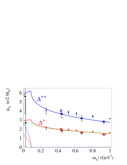
Figure 7: Pion mass dependence of the real (solid curves) and imaginary (dashed curves) parts of $\Delta^{++}$ and $\Delta^{+}$ MDMs [in nuclear magnetons]. Dashed-dotted curve is the result for the proton magnetic moment from Ref. [28]. The experimental data points for $\Delta^{++}$ and $\Delta^{+}$ (circles) are the values quoted by the PDG. Quenched lattice data are from Refs. [29] (squares) and from Ref. [30] (triangles).

The dashed-dotted curve in Fig. 7 shows the result [28] for the magnetic moment of the proton. One can see that $\mu_{\Delta^{+}}$ and $\mu_{p}$, while having very distinct behavior for small $m_{\pi}$, are approximately equal for larger values of $m_{\pi}$.

The NLO calculation, completely fixes the imaginary part of the $\gamma\Delta\Delta$ vertex. (For an alternative recent calculation of the imaginary part of the $\Delta$ MDM see Ref.[31]).

The expansion for the real part of the $\gamma\Delta\Delta$ begins with LECs from ${\mathcal{L}}^{(2)}$ which represent the isoscalar and isovector MDM couplings[9]: $\kappa_{\Delta}^{(S)}$ and $\kappa_{\Delta}^{(V)}$. A linear combination of these parameters, $\mu_{\Delta^{+}}=[3+(\kappa_{\Delta}^{(S)}+\kappa_{\Delta}^{(V)})/2](e/2M_{\Delta})$, is to be extracted from the $\gamma p\to\pi^{0}p\gamma^{\prime}$ observables. For further discussion of how this is done I, for the reason of space, have to refer to the original paper[27].

6 HB$\chi$PT vs manifestly covariant baryon $\chi$PT

The original formulation of chiral perturbation theory with nucleons is done in the manifestly Lorentz-invariant fashion[7]. However, essentially because of the use of the $\overline{MS}$ renormalization scheme, it was found violate the chiral power counting. The heavy-baryon chiral perturbation theory (HB$\chi$PT), which treats nucleons semi-relativistically, was developed to cure the power-counting problem [32]. The heavy-baryon formalism was extensively used in the previous decade and is still used sometimes. More recently, Becher and Leutwyler [33] proposed a manifestly Lorentz-invariant formulation supplemented with so-called “infrared regularization” (IR) of loops in which the chiral power-counting is manifest. The IR, however, alters the analytic structure of the loop amplitude – a very undesirable feature. At about the same time it was realized[34] that power-counting can be maintained in a manifestly covariant formalism without the IR or the heavy-baryon expansions. The original formulation[7] satisfies the power-counting provided the appropriate renormalizations of available low-energy constants are performed, such that the renormalization scale is set at the nucleon mass scale.

It since has been argued that the manifestly covariant calculations have, at least in some cases, better convergence than their heavy-baryon counterparts. This means that the convergence is improved by a resummation of terms which are required by analyticity, but are formally higher-order relativistic corrections to the non-analytic terms.

In the $\Delta$-resonance region calculations, reviewed here, the use of the manifestly covariant formalism has been seen to be of utmost importance from the viewpoint of convergence and naturalness of the theory. The same statement can be for the studies of the chiral behavior for larger than physical values of pion mass.[28, 35]

7 Summary

In the single-nucleon sector the limit of applicability of chiral perturbation theory is set by the excitation energy of the first nucleon resonance – the $\Delta$(1232). Inclusion of the $\Delta$ in the chiral Lagrangian extends the limit of applicability into the resonance energy region. The power counting of the $\Delta$ contribution depends crucially on how the $\varDelta=M_{\Delta}-M_{N}$, weighted in comparison to the other mass scales in the problem, in this case the pion mass $m_{\pi}$ and the scale of chiral symmetry breaking ${\Lambda}$.

Two different schemes exist in the literature. In the Small Scale Expansion $\varDelta\sim m_{\pi}\ll{\Lambda}$, while in the “$\delta$-expansion” $m_{\pi}\ll\varDelta\ll{\Lambda}$. I have argued that the hierarchy of scales used in the $\delta$ expansion provides a more adequate power-counting of the $\Delta$-resonance contributions. It provides a justification for “integrating out” the resonance contribution at very low energies, as well as for resummation and dominance of resonant contributions in the resonance region.

The $\delta$ expansion has already been successfully applied (at NLO) to the calculation of observables for processes such as pion-nucleon and Compton scattering, pion electroproduction and radiative pion photoproduction in the $\Delta$-resonance region. This applications show good convergence properties of this chiral EFT expansion. The use of the manifestly Lorentz-invariant formalism is seen to play an important role in naturalness of the theory.

I have also given the examples of how the chiral EFT plays here a dual role in that it allows for an extraction of resonance properties from observables and predicts their pion-mass dependence. In this way it may provide a crucial connection of present lattice QCD results to the experiment.

References

- [1] S. Weinberg, Physica A 96, 327 (1979); J. Gasser and H. Leutwyler, Annals Phys. 158, 142 (1984); Nucl. Phys. B 250, 465 (1985).
- [2] I. Caprini, G. Colangelo and H. Leutwyler, Phys. Rev. Lett. 96, 132001 (2006).
- [3] P. F. Bedaque, H. W. Hammer and U. van Kolck, Phys. Lett. B 569, 159 (2003); U. van Kolck, Nucl. Phys. A 752, 145 (2005).
- [4] H. Leutwyler, “pi pi scattering,” in these Proceedings [arXiv:hep-ph/0612112].
- [5] H. W. Hammer, N. Kalantar-Nayestanaki and D. R. Phillips, a Working Group Summary in these Proceedings [arXiv:nucl-th/0611084].
- [6] V. Pascalutsa and D. R. Phillips, Phys. Rev. C 67, 055202 (2003).
- [7] J. Gasser, M. E. Sainio and A. Svarc, Nucl. Phys. B 307, 779 (1988).
- [8] E. Jenkins and A. V. Manohar, Phys. Lett. B 259, 353 (1991).
- [9] V. Pascalutsa, M. Vanderhaeghen and S. N. Yang, Phys. Rep. (in press) [arXiv:hep-ph/0609004].
- [10] T. Hemmert, B. R. Holstein and J. Kambor, Phys. Lett. B 395, 89 (1997); J. Phys. G 24, 1831 (1998).
- [11] T. R. Hemmert, M. Procura and W. Weise, Phys. Rev. D 68, 075009 (2003).
- [12] V. Bernard, Th. Hemmert and U. G. Meißner, Phys. Lett. B 622, 141 (2005).
- [13] C. Hacker, N. Wies, J. Gegelia, S. Scherer, Phys. Rev. C 72, 055203 (2005).
- [14] G. C. Gellas et al., Phys. Rev. D 60, 054022 (1999).
- [15] T. A. Gail and T. R. Hemmert, arXiv:nucl-th/0512082.
- [16] R. P. Hildebrandt et al., Eur. Phys. J. A 20, 293 (2004); R. P. Hildebrandt, PhD Thesis (University of Munich, 2005) [arXiv:nucl-th/0512064].
- [17] C. Hanhart and N. Kaiser, Phys. Rev. C 66, 054005 (2002).
- [18] R. A. Arndt, I. I. Strakovsky, R. L. Workman, Phys. Rev. C 53, 430 (1996).
- [19] V. Pascalutsa and M. Vanderhaeghen, Phys. Rev. Lett. 95, 232001 (2005).
- [20] V. Pascalutsa and M. Vanderhaeghen, Phys. Rev. D 73, 034003 (2006).
- [21] T. A. Gail and T. R. Hemmert, in Proc. of Shape of Hadrons, eds. C. N. Papanicolas and A. M. Bernstein, AIP (2007) [arXiv:nucl-th/0610081].
- [22] V. Pascalutsa and M. Vanderhaeghen, in Proc. of Shape of Hadrons, eds. C. N. Papanicolas and A. M. Bernstein, AIP (2007) [arXiv:hep-ph/0611317].
- [23] D. Drechsel et al., Phys. Lett. B 484, 236 (2000).
- [24] D. Drechsel and M. Vanderhaeghen, Phys. Rev. C 64, 065202 (2001).
- [25] M. Kotulla et al., Phys. Rev. Lett. 89, 272001 (2002).
- [26] M. Kotulla, Talk at the Workshop Shape of Hadrons, Athens, 2006.
- [27] V. Pascalutsa and M. Vanderhaeghen, Phys. Rev. Lett. 94, 102003 (2005).
- [28] V. Pascalutsa, B. R. Holstein and M. Vanderhaeghen, Phys. Lett. B 600, 239 (2004); Phys. Rev. D 72, 094014 (2005).
- [29] D. B. Leinweber, T. Draper, R. M. Woloshyn, Phys. Rev. D 46, 3067 (1992); I. C. Cloet, D. B. Leinweber, A. W. Thomas, Phys. Lett. B 563, 157 (2003).
- [30] F. X. Lee, R. Kelly, L. Zhou and W. Wilcox, Phys. Lett. B 627, 71 (2005).
- [31] C. Hacker, N. Wies, J. Gegelia, and S. Scherer, arXiv:hep-ph/0603267.
- [32] E. Jenkins and A. V. Manohar, Phys. Lett. B 255, 558 (1991).
- [33] T. Becher and H. Leutwyler, Eur. Phys. J. C 9, 643 (1999).
- [34] J. Gegelia and G. Japaridze, Phys. Rev. D 60, 114038 (1999).
- [35] V. Pascalutsa and M. Vanderhaeghen, Phys. Lett. B 636, 31 (2006).