PITHA 06/13

hep-ph/0612290

December 21, 2006

Branching fractions, polarisation and asymmetries
of $B\to VV$ decays

Martin Beneke^a, Johannes Rohrer^a and Deshan Yang^b

^aInstitut für Theoretische Physik E, RWTH Aachen,
D–52056 Aachen, Germany
^bTheoretical Particle Physics Group (Eken), Nagoya University,
Furo-cho, Chikusa-ku, Nagoya 464-8602, Japan

We calculate the hard-scattering kernels relevant to the negative-helicity decay amplitude in ${B}$ decays to two vector mesons in the framework of QCD factorisation. We then perform a comprehensive analysis of the 34 $B\to VV$ decays, including $B_{s}$ decays and the complete set of polarisation observables. We find considerable uncertainties from weak annihilation and the non-factorisation of spectator-scattering. Large longitudinal polarisation is expected with certainty only for a few tree-dominated colour-allowed modes, which receive small penguin and spectator-scattering contributions. This allows for an accurate determination of the CKM angle $\alpha$ (or $\gamma$) from $S_{L}^{\rho\rho}$ resulting in $\alpha=(85.6^{+7.4}_{-7.3})^{\circ}$ We also emphasize that the $\rho K^{*}$ system is ideal for an investigation of electroweak penguin effects.

1 Introduction

The variety of accessible final states in $B$ decays to two mesons provides an abundant source of information on CP violation and flavour-changing processes. When the final state consists of two vector mesons, an angular analysis of the vector mesons’ decay products also provides insight into the spin structure of the flavour-changing interaction. For the $V-A$ coupling of the Standard Model, a specific pattern of the three helicity amplitudes is expected [1], such that the longitudinal polarisation fraction $f_{L}$ should be close to 1. Since $f_{L}\approx 0.5$ was first observed [2, 3] for penguin-dominated strangeness-changing decays, many theoretical papers addressed the question whether this result could be explained as a strong-interaction effect, or whether it could be reproduced within specific “New Physics” scenarios [4, 5, 6, 7, 8, 9, 10, 11, 12, 13, 14, 15, 16, 17, 18, 19, 20, 21, 22].

In this paper we revisit this question using the QCD factorisation framework [23, 24] to deal with the strong interaction in the amplitude calculation. Our study goes beyond previous ones in several respects. On the theoretical side we provide the first complete results for the hard-scattering kernels relevant to vector-vector ($VV$) final states, correcting several errors in the literature. (In fact, the only correct calculation is [6].) We also provide a more detailed discussion of the factorisation structure and power counting for the various amplitudes. It seems to have escaped attention so far that, contrary to the longitudinal polarisation amplitude and those relevant to $PP$ and $PV$ final states, the transverse polarisation amplitudes do not factorise even at leading power in the heavy-quark expansion. This, together with the high sensitvity to penguin weak-annihilation [6], implies that the calculation of polarisation observables stands on a much less solid footing than the calculation of ${B}\to PP,PV$ decays. On the phenomenological side, we provide estimates for all ${B}\to VV$ decays (including ${B}_{s}$ decays) and for all parameters that enter the angular analysis. Previous studies concentrated on single or a few decay modes and considered the longitudinal polarisation fraction $f_{L}$ only, making it often difficult to distinguish general patterns from the consequences of particular parameters choices.

The organisation of the paper is as follows: In Section 2 we summarise the definitions for the helicity amplitudes, angular variables and polarisation observables. The calculation of the ${B}\to VV$ decay amplitudes in the QCD factorisation framework is briefly reviewed in Section 3. We then discuss a few aspects of the transverse polarisation amplitudes that allow for an understanding of the main characteristics of ${B}\to VV$ phenomenology. One important conclusion from this discussion is that the analysis of $B\to VV$ decays will be much less rigorous and much more uncertain than the corresponding analysis of $B\to PP$ and $B\to VV$ modes [25]. The technical results of the calculation are summarised in an Appendix. Section 4 provides the list of input parameters, an overview of the flavour amplitude parameters with theoretical uncertainties, and a classification of the 34 $B\to VV$ decay channels, which guides the subsequent numerical analysis. We begin the analysis in Section 5 with a discussion of branching fractions, CP asymmetries and polarisation observables of the nine tree-dominated decays. Among these the four colour-allowed modes can be well predicted. In particular, we show that the time-dependent CP asymmetry measurement in $B^{0}\to\rho^{+}\rho^{-}$ leads to one of the most accurate determinations of the CKM angle $\gamma$. In Section 6 we turn to the 14 colour-allowed penguin-dominated decay modes. It will be seen that theoretical calculations allow for large transverse polarisation within large uncertainties. This suggests to determine the transverse penguin amplitude from data using the well-measured $\phi K^{*}$ modes. This approach is used to sharpen the predictions for the remaining decay modes in this class. The analysis concludes in Section 7 with a brief discussion of the remaining penguin-dominated modes, and decays that occur only through weak annihilation. Section 8 summarises our main results and conclusions.

2 Helicity amplitudes and polarisation observables

We consider a ${B}$ meson with four-momentum $p_{B}$ and mass $m_{B}$ decaying into two light vector mesons $V_{1}(p_{1},\eta^{*})$, $V_{2}(p_{2},\epsilon^{*})$ with masses $m_{1,2}$ of order $\Lambda_{\text{QCD}}$. The decay amplitude can be decomposed into three scalar amplitudes $S_{1,2,3}$ according to

$$\mathcal{A}_{{B}\to V_{1}V_{2}}=i\eta^{*\mu}\epsilon^{*\nu}\left(S_{1}\,g_{\mu\nu}-S_{2}\,\frac{p_{B\mu}p_{B\nu}}{m_{B}^{2}}+S_{3}\,i\varepsilon_{\mu\nu\rho\sigma}\frac{p_{1}^{\rho}p_{2}^{\sigma}}{p_{1}{\cdot}p_{2}}\right).$$ (1)

with convention $\varepsilon_{0123}=1.$ Alternatively, one can choose a basis of amplitudes describing decays to final state particles with definite helicity

$$\mathcal{A}_{0} =\mathcal{A}({B}\to V_{1}(p_{1},\eta_{0}^{*})V_{2}(p_{2},\epsilon_{0}^{*}))=\frac{im_{B}^{2}}{2m_{1}m_{2}}\left(S_{1}-\frac{S_{2}}{2}\right)$$ (2)

$$\mathcal{A}_{\pm} =\mathcal{A}({B}\to V_{1}(p_{1},\eta_{\pm}^{*})V_{2}(p_{2},\epsilon_{\pm}^{*}))=i\,(S_{1}\mp S_{3}).$$

or use the transversity amplitudes, where $\mathcal{A}_{\pm}$ are replaced by $\mathcal{A}_{\parallel}=(\mathcal{A}_{+}+\mathcal{A}_{-})/\sqrt{2}$ and $\mathcal{A}_{\perp}=(\mathcal{A}_{+}-\mathcal{A}_{-})/\sqrt{2}$, corresponding to linearly polarised final states. We choose $\vec{p}_{2}$ to be directed in positive $z$-direction in the ${B}$ meson rest frame, and the polarisation four-vectors of the light vector mesons such that in a frame where both light mesons have large momentum along the $z$-axis, they are given by $\epsilon_{\pm}^{\mu}=\eta_{\mp}^{\mu}=(0,\pm 1,i,0)/\sqrt{2}$, and $\epsilon_{0}^{\mu}=p_{2}^{\mu}/m_{2}$, $\eta_{0}^{\mu}=p_{1}^{\mu}/m_{1}$. Here and thoughout the paper we neglect corrections $m_{1,2}^{2}/m_{B}^{2}$ quadratic in the light meson masses. Thus $p_{1,2}^{\mu}=m_{B}n_{\mp}^{\mu}/2$ with $n_{\pm}^{\mu}=(1,0,0,\pm 1)$. Our conventions imply the identity

$$i\varepsilon_{\mu\nu\rho\sigma}\epsilon_{\pm}^{*\rho}n_{+}^{\sigma}=(\mp 1)\,\left(n_{+\mu}\epsilon_{\pm\nu}^{*}-n_{+\nu}\epsilon_{\pm\mu}^{*}\right).$$ (3)

Experimentally, the magnitudes and relative phases of the various amplitudes are extracted from the angular distributions of the vector resonance decay products. The full angular dependence of the cascade where both vector mesons decay into pseudoscalar particles is given by [1]

$$\begin{split}\frac{d{\Gamma_{{B}\to V_{1}V_{2}\to\ldots}}}{d{\cos\vartheta_{1}}d{\cos\vartheta_{2}}d{\varphi}}&\,\propto\,\left|\mathcal{A}_{0}\right|^{2}\cos^{2}\vartheta_{1}\cos^{2}\vartheta_{2}+\frac{1}{4}\sin^{2}\vartheta_{1}\sin^{2}\vartheta_{2}\left(\left|\mathcal{A}_{+}\right|^{2}+\left|\mathcal{A}_{-}\right|^{2}\right)\\ &\mathrel{\hphantom{\propto}}-\cos\vartheta_{1}\sin\vartheta_{1}\cos\vartheta_{2}\sin\vartheta_{2}\left[\mathrm{Re}\left(\mathrm{e}^{-i\varphi}\mathcal{A}_{0}\mathcal{A}_{+}^{*}\right)+\mathrm{Re}\left(\mathrm{e}^{+i\varphi}\mathcal{A}_{0}\mathcal{A}_{-}^{*}\right)\right]\\ &\mathrel{\hphantom{\propto}}+\frac{1}{2}\sin^{2}\vartheta_{1}\sin^{2}\vartheta_{2}\,\mathrm{Re}\left(\mathrm{e}^{2i\varphi}\mathcal{A}_{+}\mathcal{A}_{-}^{*}\right),\end{split}$$ (4)

where $\varphi$ measures the angle between the decay planes of the two vector mesons in the ${B}$ meson rest frame, and $\vartheta_{1,2}$ are the angles between the direction of motion of one of the $V_{1,2}\to PP$ pseudoscalar final states and the inverse direction of motion of the ${B}$ meson as measured in the $V_{1,2}$ rest frame, see Figure 1. The omitted proportionality factor is such that one obtains the decay rate $\Gamma({B}\to V_{1}V_{2})$ when $\cos\vartheta_{1}$ and $\cos\vartheta_{2}$ are integrated from $-1$ to $1$, and $\varphi$ from 0 to $2\pi$.

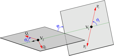
Figure 1: Decay kinematics in the rest frame of $V_{1}$.

Thus, any given ${B}\to VV$ decay allows us to define five observables corresponding to the three magnitudes and two relative phases of the helicity amplitudes, or the five angular coefficients in (4). In experimental analyses, observables are preferably defined in terms of the transversity amplitudes as they have definite CP transformation properties. A typical set of observables consists of the branching fraction, two out of the three polarisation fractions $f_{L},f_{\parallel},f_{\perp}$, and two phases $\phi_{\parallel}$, $\phi_{\perp}$, where

$$f^{{B}}_{L,\parallel,\perp}=\frac{\left|\mathcal{A}_{0,\parallel,\perp}\right|^{2}}{\left|\mathcal{A}_{0}\right|^{2}+\left|\mathcal{A}_{\parallel}\right|^{2}+\left|\mathcal{A}_{\perp}\right|^{2}},\qquad\qquad\phi^{{B}}_{\parallel,\perp}=\arg\frac{\mathcal{A}_{\parallel,\perp}}{\mathcal{A}_{0}}.$$ (5)

It is conventional to combine the five observables of some ${B}\to VV$ decay with those of its CP-conjugate $\bar{{B}}$ decay, and to quote the ten resulting observables as CP-averages and CP-asymmetries. We denote $\bar{{B}}$ decay helicity amplitudes as $\bar{\mathcal{A}}_{h}$ and define the corresponding transversity amplitudes as $\bar{\mathcal{A}}_{\parallel/\perp}=(\bar{\mathcal{A}}_{-}\pm\bar{\mathcal{A}}_{+})/\sqrt{2}$, so that $\mathcal{A}_{\parallel/\perp}=\bar{\mathcal{A}}_{\parallel/\perp}$ in the absence of CP violation. Observables $f_{h}^{\bar{{B}}},\phi^{\bar{{B}}}_{h}$ are then defined as in (5), and CP averages and asymmetries are calculated by

$$f_{h}=\frac{1}{2}\left(f_{h}^{\bar{{B}}}+f_{h}^{{B}}\right),\qquad A_{\mathrm{CP}}^{h}=\frac{f_{h}^{\bar{{B}}}-f_{h}^{{B}}}{f_{h}^{\bar{{B}}}+f_{h}^{{B}}}$$ (6)

($h=L,\parallel,\perp$) for the polarisation fractions and

$$\phi_{h} \equiv\phi^{\bar{{B}}}_{h}-\Delta\phi_{h}\pmod{2\pi}$$ (7)

$$\equiv\phi^{{B}}_{h}+\Delta\phi_{h}\pmod{2\pi},\qquad-\frac{\pi}{2}\leq\Delta\phi_{h}<\frac{\pi}{2}$$

($h=\,\parallel,\perp$) for the phase observables $\phi_{h}$ and $\Delta\phi_{h}$. The implicit definition (7) ensures that the CP-averaged phase is the geometrical bisection of the acute angle enclosed by $\phi^{{B}}$ and $\phi^{\bar{{B}}}$; the magnitude of this angle is $2\left|\Delta\phi\right|$. More explicitly, the averaged quantities can be obtained as

$$\phi_{h} =\frac{1}{2}\left(\phi^{\bar{{B}}}_{h}+\phi^{{B}}_{h}\right)-\pi\cdot\operatorname{sign}\left(\phi^{\bar{{B}}}_{h}+\phi^{{B}}_{h}\right)\theta\left(\left|\phi^{\bar{{B}}}_{h}-\phi^{{B}}_{h}\right|-\pi\right),$$ (8)

$$\Delta\phi_{h} =\frac{1}{2}\left(\phi^{\bar{{B}}}_{h}-\phi^{{B}}_{h}\right)+\pi\cdot\theta\left(\left|\phi^{\bar{{B}}}_{h}-\phi^{{B}}_{h}\right|-\pi\right)\pmod{2\pi}.$$

Our phase convention for the amplitudes and definition of observables is compatible with that used in the relevant publications of the BaBar and Belle collaborations (for example in [26, 28, 29, 30]), except for the sign of $\mathcal{A}_{0}$ relative to the transverse amplitudes, which leads to an offset of $\pi$ for $\phi_{\parallel/\perp}$. We favour the above convention, because it implies $\phi_{\parallel}=\phi_{\perp}=0$ and $\Delta\phi_{\parallel}=\Delta\phi_{\perp}=0$ at leading order, where all strong phases are zero.

3 ${B}\to VV$ amplitudes

The decay amplitudes follow from the matrix elements $\langle V_{1}V_{2}|\mathcal{H}_{\text{eff}}|\bar{{B}}\rangle$ of the effective Hamiltonian (conventions as in [31])

$$\mathcal{H}_{\text{eff}}=\frac{G_{\mathrm{F}}}{\sqrt{2}}\sum_{p=u,c}\lambda^{(D)}_{p}\left\{C_{1}Q_{1}^{p}+C_{2}Q_{2}^{p}+\!\!\sum_{i=3,\ldots 10,7\gamma,8g}\!\!C_{i}Q^{p}_{i}\right\}+\mathrm{h.\,c.}$$ (9)

with $D\in\{d,s\}$ and $\lambda^{(D)}_{p}=V_{pb}V^{*}_{pD}$. A quark model [1] or naive factorisation analysis indicates a hierarchy of helicity amplitudes

$$\bar{\mathcal{A}}_{0}:\bar{\mathcal{A}}_{-}:\bar{\mathcal{A}}_{+}=1:\frac{\Lambda_{\text{QCD}}}{m_{b}}:\left(\frac{\Lambda_{\text{QCD}}}{m_{b}}\right)^{\!2}$$ (10)

for $\bar{{B}}$ meson decays. (For ${B}$ decays exchange $-\leftrightarrow+$.) This is a consequence of the left-handedness of the weak interaction and the fact that high-energy QCD interactions conserve helicity.

In naive factorisation one considers only the four-quark operators in $\mathcal{H}_{\text{eff}}$ and approximates their matrix elements by the matrix elements of two currents [32]. The helicity amplitudes $\mathcal{A}_{\bar{{B}}\to V_{1}V_{2}}^{h}$ are proportional to

$$A^{h}_{V_{1}V_{2}}\equiv\frac{G_{\mathrm{F}}}{\sqrt{2}}\;\langle V^{h}_{1}|(\bar{q}_{s}b)_{V-A}|\bar{{B}}_{q_{s}}\rangle\langle V^{h}_{2}|(\bar{q}q^{\prime})_{V}|0\rangle$$ (11)

in this approximation. Evaluating this expression (conventions for the form factors as in [33]) we obtain

$$A^{0}_{V_{1}V_{2}} =\frac{iG_{\mathrm{F}}}{\sqrt{2}}m_{B}^{2}f_{V_{2}}A_{0}^{{B}\to V_{1}}(0),\qquad A^{\pm}_{V_{1}V_{2}}=\frac{iG_{\mathrm{F}}}{\sqrt{2}}m_{B}m_{2}f_{V_{2}}F_{\pm}^{{B}\to V_{1}}(0)$$ (12)

with the definitions

$$F_{\pm}^{{B}\to V_{1}}(q^{2})\equiv(1+\frac{m_{1}}{m_{B}})A_{1}^{{B}\to V_{1}}(q^{2})\mp(1-\frac{m_{1}}{m_{B}})V^{{B}\to V_{1}}(q^{2}).$$ (13)

The transverse amplitudes $A^{\pm}_{V_{1}V_{2}}$ are suppressed by a factor $m_{2}/m_{B}$ relative to $A^{0}_{V_{1}V_{2}}$. In addition, the axial-vector and vector contributions to $F_{+}^{{B}\to V_{1}}(0)$ cancel in the heavy-quark limit, due to an exact form factor relation [33, 34]. Thus $F_{-}/A_{0}\sim 1$, $F_{+}/A_{0}\sim\mathcal{O}(\Lambda_{\text{QCD}}/m_{B})$, and (10) follows.

The dominance of the longitudinal amplitude indicated by (10) leads to the well-known expectation that $f_{L}$ should be close to unity. Experimental data for penguin-dominated ${B}$ decays is in conflict with this expectation thus motivating theoretical studies beyond the naive-factorisation approximation.

3.1 The QCD factorisation approach for ${B}\to VV$

We use the QCD factorisation approach [23, 24] to compute the matrix elements $\langle V_{1}V_{2}|Q_{i}|\bar{{B}}\rangle$ of the effective Hamiltonian. In this framework they can be expressed (at leading power in an expansion of the amplitude in $\Lambda_{\text{QCD}}/m_{B}$) in terms of form factors, meson light-cone distribution amplitudes and perturbatively calculable hard scattering kernels. In condensed notation, the factorisation formula reads

$$\begin{split}\langle V_{1}V_{2}|Q_{i}|\bar{{B}}\rangle=&\left(F^{{B}\to V_{1}}\,T^{I}_{i}\ast f_{V_{2}}\Phi_{V_{2}}+[V_{1}\leftrightarrow V_{2}]\right)+T^{II}_{i}\ast f_{B}\Phi_{{B}}\ast f_{V_{1}}\Phi_{V_{1}}\ast f_{V_{2}}\Phi_{V_{2}},\end{split}$$ (14)

where the star products imply an integration over light-cone momentum fractions. In addition the framework contains estimates of some power corrections, which usually cannot be computed rigorously.

We follow closely the scheme developed in [25] for $B\to PP,PV$ decays to match contributions to the hard-scattering kernels $T^{I,II}_{i}$ on terms involving products of flavour coefficients $\alpha_{i}^{p,h}(V_{1}V_{2})$ and factorised matrix elements $A^{h}_{V_{1}V_{2}}$. The longitudinal amplitude $h=0$ can be deduced from the results given in [25]. For the analysis of the present paper we calculated the transverse helicity amplitudes. In the following we describe the basic results and main differences with respect to the longitudinal amplitude; the expressions for the hard-scattering functions are given in the Appendix.

Non-leptonic decay amplitudes are sums of products of CKM factors, Wilson coefficients from (9) and matrix elements (14) of operators with different flavours. It is convenient to organise the amplitudes according to flavour. Thus, one writes for example,

$$\sqrt{2}\,{\cal A}_{{B}^{-}\to\rho^{0}K^{*-}}^{h} = \sum_{p=u,c}\lambda_{p}^{(s)}\bigg{\{}A^{h}_{\rho\bar{K}^{*}}\left[\delta_{pu}\,(\alpha_{1}^{h}+\beta_{2}^{h})+\alpha_{4}^{p,h}+\alpha_{4,{\rm EW}}^{p,h}+\beta_{3}^{p,h}+\beta_{3,{\rm EW}}^{p,h}\right]$$ (15)

$$+\,A^{h}_{\bar{K}^{*}\rho}\Big{[}\delta_{pu}\,\alpha_{2}^{h}+\frac{3}{2}\alpha_{3,{\rm EW}}^{p,h}\Big{]}\bigg{\}}.$$

In naive factorisation, the flavour coefficients $\alpha_{i}^{p,h}(V_{1}V_{2})$ are linear combinations of Wilson coefficients $C_{i}$. In QCD factorisation, they include non-factorisable loop effects and spectator-scattering. The $\beta_{i}^{p,h}$ coefficients parameterise weak annihilation amplitudes. The decomposition of the amplitudes for the 34 $VV$ final states in terms of these quantities follows from the $PV$ expressions given in [25] with obvious replacements of pseudoscalar by vector mesons. The $\alpha_{i}$ relate to the coefficients $a_{i}$ used in the older factorisation literature as follows (helicity indices and $V_{1}V_{2}$ arguments suppressed):

$$\begin{split}\alpha_{1}&=a_{1}\\ \alpha_{2}&=a_{2}\end{split}\qquad\begin{split}\alpha^{p}_{3}&=a^{p}_{3}+a^{p}_{5}\\ \alpha^{p}_{3,\mathrm{EW}}&=a^{p}_{9}+a^{p}_{7}\end{split}\qquad\begin{split}\alpha^{p}_{4}&=a^{p}_{4}-r_{\chi}^{V_{2}}a^{p}_{6}\\ \alpha^{p}_{4,\mathrm{EW}}&=a^{p}_{10}-r_{\chi}^{V_{2}}a^{p}_{8},\end{split}$$ (16)

where we have used the notation

$$r_{\chi}^{V}\equiv\frac{2m_{V}}{m_{b}}\frac{f_{V}^{\perp}}{f_{V}}.$$ (17)

The explicit expressions for the negative-helicity coefficients $a_{i}^{p-}$ and the transverse weak annihilation amplitudes are collected in the Appendix. Beyond leading order the $a_{i}^{p-}$ are sums of vertex corrections, penguin contractions, and spectator-scattering contributions, see (53). Most of the relevant hard-scattering functions have been calculated before. In [4, 5, 12, 13, 16] results for all three of these contributions have been given. We do not find agreement with these results, however. As far as we understand, the origin of the discrepancy is that the authors of these papers use an incorrect projection on the light-cone distribution amplitudes of transversely polarised vector mesons, which neglects the transverse-momentum derivative terms in (52). An exception is [13], which does state the correct projector, but the results still differ from ours, particularly for the spectator-scattering contributions. Kagan [6] has calculated the QCD penguin contractions, spectator-scattering terms as well as the weak annihilation amplitudes, but did not consider the vertex contractions. We confirm his results on the penguin contractions and QCD penguin annihilation, for which explicit expressions were given in the paper.

3.2 Anatomy of transverse amplitudes

The NLO calculation of the negative-helicity amplitude is quite similar to the calculation of the longitudinal amplitude. The result exhibits, however, some qualitative differences which have important consequences for the phenomenology of ${B}\to VV$ decays. In this section we explain the non-factorisation of the negative-helicity amplitude; that the positive-helicity amplitude cannot be calculated in an analogous manner; that the amplitude hierarchy (10) is violated by electromagnetic effects; that penguin annihilation is comparatively more significant for transverse polarisation than longitudinal polarisation penguin amplitudes.

3.2.1 Non-factorisation of spectator scattering

The factorisation formula (14) contains two structurally different terms, the first of which is dominated by soft interactions within the ${B}\to M_{1}$ transitions. These are absorbed into the QCD form factor. The second term stands for interactions where a hard (more precisely, hard-collinear) interaction with the spectator quark in the ${B}$ meson takes place. Both terms are of the same order in the heavy-quark expansion. This remains true for the transverse polarisation amplitudes, but now one finds that the convolution integrals over the light-cone distribution amplitudes are logarithmically divergent due to the occurence of the integral

$$\int_{0}^{1}dx\,\frac{\phi_{1}^{\perp}(x)}{(1-x)^{2}},$$ (18)

see (61), (62). This endpoint divergence at $x=1$ signals that the presumed factorisation of spectator-scattering does not hold even at leading power. A similar effect occurs in the ${B}\to PP,PV$ and longitudinal ${B}\to VV$ amplitude only when one attempts to calculate power corrections by applying the light-cone projection including twist-3 terms. It is perhaps not surprising that this divergence is obtained at leading-power for the transverse amplitude, since the entire amplitude is formally a twist-3 term. (This is the origin of the power suppression of the transverse amplitudes relative to the longitudinal amplitude.) Factorisation-violation at the leading power implies that the calculation of transverse polarisation amplitudes is on a much less solid footing than of the other amplitudes, and often should be considered more as an estimate. In practice, we find that the non-factorisation of spectator-scattering is only significant for the colour-suppressed tree and the flavour-singlet QCD penguin amplitudes, where the (regulated) divergent integral is multiplied by a large Wilson coefficient. The fact that there are endpoint divergences in the spectator-scattering contribution to the transverse helicity amplitudes has been observed in previous calculations, but its significance for the theoretical status of the factorisation approach and its phenomenological implications have not been sufficiently emphasized.

3.2.2 The positive-helicity amplitude

The calculation of the kernels $T^{I}_{i}$ in (14) can be interpreted as matching the operators $Q_{i}$ to four-quark operators with field content $[\bar{\chi}\chi][\bar{\xi}h_{v}]$ in soft-collinear effective theory [35]. The field $\chi$ describes collinear quarks moving in the direction of $V_{2}$, the meson that does not pick up the spectator quark, and satisfies $\not\!n_{+}\chi=0$. The leading quark bilinears that have non-vanishing overlap with $\langle V_{2}|$ are

$$\bar{\chi}\!\not\!n_{-}(1\mp\gamma_{5})\chi,\quad\bar{\chi}\!\not\!n_{-}\gamma_{\perp}^{\mu}(1\pm\gamma_{5})\chi.$$ (19)

The subscript $\perp$ denotes projection of a Lorentz vector on the plane transverse to the two light-cone vectors $n_{\mp}$. The first operator overlaps only with the longitudinal polarisation state of $V_{2}$, the second only with a transverse vector meson. However, the second operator is not generated by the $V-A$ interactions of the Standard Model, at least up to the one-loop level. Hence the transverse amplitudes arise from power-suppressed operators $\mathcal{O}_{\perp}=[\bar{\chi}D_{\perp}\chi][\bar{\xi}h_{v}]$. (In terms of the light-cone projector (52) this statement implies that the leading term in the first line does not contribute for $V-A$ interactions, leaving the twist-3 terms in the second and third line. Since $\mathcal{O}_{\perp}$ contains transverse momentum derivatives, one must keep the transverse momenta of partons collinear to $V_{2}$; this explains why the transverse-momentum derivative terms in the projector are required.) The left-handedness of the weak interactions implies that operators of this form contribute only to the negative-helicity amplitude. The positive-helicity amplitude appears first in yet higher-dimensional operators such as $[\bar{\chi}D_{\perp}\chi][\bar{\xi}D_{\perp}h_{v}]$. To match to such operators one must keep the transverse momentum of the quark lines collinear to both mesons non-zero. Such a calculation has not yet been done, and therefore all calculations of the positive-helicity amplitude in the literature must be regarded as incomplete. It is even possible that for the positive-helicity amplitude no useful factorisation formula holds even for the non-spectator-scattering terms in (14).

It follows that the positive-helicity amplitude is power-suppressed relative to the negative one, and should be set to zero in the absence of any consistent calculation of this power correction. Within this approximation, $\bar{\mathcal{A}}_{+}=\mathcal{A}_{-}=0$, there are only two rather than four independent polarisation observables, since

$$f_{\parallel}=f_{\perp},\qquad\qquad\phi_{\parallel}=\phi_{\perp}.$$ (20)

Similarly identities for the corresponding CP asymmetries hold. It should be noted that these identities are non-trivial consequences of the $V-A$ nature of the weak interactions and of factorisation, and it is therefore worthwhile to test them experimentally.

In our analysis we proceed as follows: we assume the naive-factorisation expression for the positive-helicity amplitude $\bar{\mathcal{A}}_{+}$ and allow the form factor to vary within the range $F_{+}^{{B}\to V_{1}}=0\pm 0.06$. Thus, we allow a small variation of $\bar{\mathcal{A}}_{+}$ around zero to estimate the error from neglecting this power correction. We note that QCD sum rule results for the form factors give $F_{+}$ values consistent with zero [36, 37].

3.2.3 Violation of the amplitude hierarchy

In the previous paragraphs we explained the origin of the amplitude hierarchy (10). However, when electromagnetic effects are included, a transverse polarisation amplitude can be generated by a short-distance transition to a vector meson and a photon with small virtuality which subsequently converts to a vector meson [20]. This transition is enhanced by a factor $(m_{B}/\Lambda_{\text{QCD}})^{2}$ due to the large photon propagator, resulting in the parametric relation

$$\bar{\mathcal{A}}_{0}:\bar{\mathcal{A}}_{-}:\bar{\mathcal{A}}_{+}=1:\frac{\alpha_{\mathrm{em}}m_{b}}{\Lambda_{\text{QCD}}}:\alpha_{\mathrm{em}}.$$ (21)

Thus, formally, the negative-helicity amplitude is leading in the heavy-quark limit. Technically, this is related to the existence of the operator $[A_{\gamma_{\perp}}][\bar{\xi}h_{v}]$, which contributes only to the transverse amplitude, and which is enhanced relative to $[\bar{\chi}\chi][\bar{\xi}h_{v}]$. In the Standard Model the leading effect of this type involves the electromagnetic-dipole operator in the effective Hamiltonian. As a consequence the colour-allowed electroweak penguin amplitude $\alpha_{3\,\rm\mathrm{EW}}^{p-}$ is completely different from its naive-factorisation value. Our calculations include this contribution, which has already been discussed specifically in [20].

3.2.4 Penguin weak annihilation

Weak annihilation is a power correction not included in (14), since it does not factorise due to endpoint divergences in the convolution integrals. The effect is often estimated by a parameterisation suggested in [31], where the endpoint-divergences are regulated by a cut-off. In this model one finds that the most important annihilation effect is a penguin annihilation amplitude that is phenomenologically indistinguishable from the QCD penguin amplitude. These general observations also hold for the transverse polarisation amplitudes. In particular, the weak annihilation contribution to the negative-helicity amplitude is a power correction relative to the leading, factorisable contributions to this amplitude. Yet, as found in [6], the effect is numerically much larger than in ${B}\to PP,PV$ decays, and perhaps so large that a theoretical calculation of the negative-helicity QCD penguin amplitude is no longer possible.

To explain this point, we consider the QCD penguin amplitude

$$P^{h}=A^{h}_{V_{1}V_{2}}\left[\alpha_{4}^{h}+\beta_{3}^{h}\right],$$ (22)

and compare the $h=0$ and $h=-$ amplitudes. Here $\alpha_{4}^{h}$ are the QCD penguin contributions, and $\beta_{3}^{h}$ the penguin annihilation contributions. For the longitudinal amplitude $\beta_{3}^{0}$ is $\Lambda_{\text{QCD}}/m_{b}$ suppressed relative to $\alpha_{4}^{0}$, but it turns out that numerically the largest effect arises from a $(\Lambda_{\text{QCD}}/m_{b})^{2}$ term, which has a large colour factor and Wilson coefficient. This particular contribution is not suppressed by the extra factor of $\Lambda_{\text{QCD}}/m_{b}$ in the negative-helicity amplitude. One finds $A^{-}_{V_{1}V_{2}}\beta_{3}^{-}\approx A^{0}_{V_{1}V_{2}}\beta_{3}^{0}$, while $A^{-}_{V_{1}V_{2}}\alpha_{4}^{-}\ll A^{0}_{V_{1}V_{2}}\alpha_{4}^{0}$ due to the power suppression of $A^{-}_{V_{1}V_{2}}$ with respect to $A^{0}_{V_{1}V_{2}}$. Thus, relative to $\alpha_{4}^{h}$ the numerical effect of $\beta_{3}^{h}$ is a factor of $m_{b}/\Lambda_{\text{QCD}}$ larger for the negative-helicity amplitude than for the longitudinal amplitude (but still power-suppressed since the suppression was $(\Lambda_{\text{QCD}}/m_{b})^{2}$ for $h=0$).

The following numerical estimates illustrate this point. We consider the $p=c$, $h=0,-$ helicity amplitudes for $\rho K^{*}$, and also the $\pi K$ amplitude for comparison. The imaginary parts of the amplitudes are neglected, since they are not important for this discussion. We then find

$$\alpha_{4}^{c}(\pi\bar{K})+\beta_{3}^{c}(\pi\bar{K}) =\;\;-0.09-\big{\{}0.02\,[-0.01,0.05]\big{\}},$$ (23)

$$\alpha_{4}^{c0}(\rho\bar{K}^{*})+\beta_{3}^{c0}(\rho\bar{K}^{*}) =\;\;-0.03-\big{\{}0.00\,[-0.00,0.00]\big{\}},$$

$$\alpha_{4}^{c-}(\rho\bar{K}^{*})+\beta_{3}^{c-}(\rho\bar{K}^{*}) =\;\;-0.05-\big{\{}0.03\,[-0.04,0.10]\big{\}}.$$

The numbers in curly brackets refer to $\beta_{3}^{p,h}$. The first number in brackets is the default value, while the interval provides the range allowed by the parameterisation adopted in [31]. We observe a (presumably accidental) cancellation in the longitudinal annihilation amplitude. What is significant is the difference in the range of the interval relative to $\alpha_{4}^{c,h}$ for the negative-helicty $VV$ amplitude vs. the $PP$ amplitude. In particular, the annihilation contribution $\beta_{3}^{c-}$ may be significantly larger than the QCD penguin amplitude $\alpha_{4}^{c-}$ for the negative-helicity amplitude. We can also compare the $h=-$ and $h=0$ amplitudes,

$$\frac{P^{-}}{P^{0}}\approx\frac{A^{-}_{\rho K^{*}}}{A^{0}_{\rho K^{*}}}\frac{\alpha_{4}^{c-}+\beta_{3}^{c-}}{\alpha_{4}^{c,0}}\approx\frac{0.05+[-0.04,0.10]}{0.12},$$ (24)

where we used $A^{-}_{\rho K^{*}}/A^{0}_{\rho K^{*}}\approx 1/4$. This shows that $P^{-}$ could be as large as $P^{0}$, if annihilation is maximal. Thus, for penguin-dominated decays, a longitudinal polarisation fraction $f_{L}$ around 0.5 is not ruled out.

Let us summarise these and a few further observations on the role of weak annihilation in ${B}\to VV$ decays:

• The annihilation contribution to the longitudinal penguin amplitude is small, perhaps due to an accidental cancellation.

• The annihilation contribution to the negative-helicity penguin amplitude can (but need not) be very large, possibly leading to significant transverse polarisation in penguin-dominated decays.

• No such enhancement is observed for the annihilation contribution to the tree amplitudes, hence tree-dominated decays should be predominantly longitudinally polarised.

• We also calculated the weak annihilation contribution to the positive-helicity amplitude, and find that the large contribution to $\beta_{3}^{+}$ is absent. Hence there is no evidence for large corrections to (20) even for penguin-dominated decays.

It should be clear that these statements assume that the parameterisation adopted in [31] reproduces correctly the qualitative features of the weak annihilation amplitudes.

4 Input and overview

4.1 Input parameters

QCD scale and running quark masses [GeV]
$\Lambda_{\text{QCD}}=\Lambda_{\overline{\mathrm{MS}}}^{(5)}$	$m_{b}(m_{b})$	$m_{c}$	$m_{s}(2\,\text{GeV})$	$m_{q}/m_{s}$
0.225	4.2	$1.3\pm 0.2$	$0.09\pm 0.02$	0.0413
CKM parameters
$\lambda$	$|V_{cb}|$	$|V_{ub}/V_{cb}|$	$\gamma$
$0.225$	$0.0415\pm 0.0010$	$0.085^{+0.025}_{-0.015}$	$(70\pm 20)^{\circ}$
${B}$ meson parameters		${B}^{-}$	$\bar{{B}}^{0}$	$\bar{{B}}_{s}$
lifetime	$\tau$ [ps]	1.64	1.53	1.46
decay constant	$f_{{B}}$ [MeV]	$210\pm 20$		$240\pm 20$
	$\lambda_{B}$ [MeV]	$200^{+250}_{-0}$		$200^{+250}_{-0}$
Light meson decay constants and Gegenbauer moments
	${\rho}$	$\bar{{K}}^{*}$	${\omega}$	${\phi}$
$f$ [MeV]	$209\pm 1$	$218\pm 4$	$187\pm 3$	$221\pm 3$
$f^{\perp}$ [MeV]	$150\pm 25$	$175\pm 25$	$150\pm 25$	$175\pm 25$
$\alpha_{1}$, $\alpha_{1,\perp}$	0	$0.06\pm 0.06$	0	0
$\alpha_{2}$, $\alpha_{2,\perp}$	$0.1\pm 0.2$	$0.1\pm 0.2$	$0.0\pm 0.3$	$0.0\pm 0.3$

Form factors for vector mesons at $q^{2}=0$
	${B}\to{\rho}$	${B}\to{K}^{*}$	${B}\to{\omega}$	${B}_{s}\to\bar{{K}}^{*}$	${B}_{s}\to{\phi}$
$A_{0}$	$0.30^{+0.07}_{-0.03}$	$0.39\pm 0.06$	$0.25^{+0.07}_{-0.03}$	$0.33\pm 0.05$	$0.38^{+0.10}_{-0.02}$
$F_{-}$	$0.55\pm 0.06$	$0.68\pm 0.07$	$0.50\pm 0.05$	$0.53\pm 0.05$	$0.65^{+0.14}_{-0.00}$
$F_{+}$	$0.00\pm 0.06$	$0.00\pm 0.06$	$0.00\pm 0.06$	$0.00\pm 0.06$	$0.00\pm 0.06$

Table 1: Summary of theoretical input parameters. All scale-dependent quantities refer to $\mu=2$ GeV unless indicated otherwise. $m_{q}=(m_{u}+m_{d})/2$.

The values of the Standard Model and hadronic input parameters are listed in Table 1. When we compare $B\to VV$ modes to decays with pions in the final state, the additional pion parameters are $f_{\pi}=131\,$MeV, $\alpha_{2}(2\,\mbox{GeV})=0.2\pm 0.15$, $f_{+}^{B\pi}(0)=0.25\pm 0.05$. (The light quark mass values reported in the Table are only needed for the computation of the pion decay amplitudes.) Relative to the analysis of $PV$ final states [25] we have implemented several minor parameter modifications (Wolfenstein parameter $\lambda$, $|V_{cb}|$, $B$ meson lifetimes and decay constants, Gegenbauer moments of light-meson light-cone distribution amplitudes), which reflect new measurements or improved calculations, but individually have little impact on the calculation of non-leptonic decay amplitudes. A more important change concerns the treatment of $|V_{ub}|$ and the $B$ meson parameter $\lambda_{B}$, where we (roughly) stick to the same ranges as before, but choose smaller default values. These values lead to a good agreement of theoretical calculations with the observed $B\to\pi\pi$ transitions as already noted in [25]. Regarding the value of $|V_{ub}|$ we note that our default value correspnds to the one that is favoured by exclusive semi-leptonic $b\to u$ transitions, which is smaller than the one from the inclusive decays (see [38] for the most recent discussion). We shall see below that the tree-dominated $B\to\rho\rho$ modes also support this small value unless the $B\to\rho$ form factors are unacceptably small, so all exclusive decays (semi-leptonic, non-leptonic PP, PV and VV modes) seem to consistently favour small $|V_{ub}|$. The default value we adopt for $\lambda_{B}$ is significantly smaller than the value obtained from QCD sum rule calculations [39, 40], which we use to define the upper limit of this parameter’s range. Some of the longitudinal and negative helicity $B\to V$ form factors have changed considerably since the publication of [25] due to the update of the QCD sum rule calculation [41]. Our new values follow [41], but in some cases a smaller form factor is adopted to improve the description of data. The smaller values are compatible with [41] within theoretical errors; in these cases, however, the theoretically allowed parameter range becomes asymmetric around the default value. The positive-helicity form factors are set to $0.00\pm 0.06$ (see Sect.3.2.2). The renormalization scales are treated as in [25] and $\mu$ is varied from $m_{b}/2$ to $2m_{b}$. The Wilson coefficients $C_{i}$ are tabulated in [31].

In addition to the well-defined hadronic parameters, the predictions of QCD factorisation depend on the model parameters $X_{H}$ and $X_{A}$, $X_{L}$ (see [31] and the Appendix for their definition). In contrast to all previous QCD factorisation calculations there is model-dependence even at leading power in the heavy quark expansion for the transverse amplitudes due to an endpoint divergence in spectator scattering (see Sect. 3.2.1). This is parameterised by

$$X_{H}=\left(1+\varrho_{H}\,e^{i\varphi_{H}}\right)\ln\frac{m_{B}}{\Lambda_{h}}\,;\qquad\Lambda_{h}=0.5\,\mbox{GeV}\,,$$ (25)

with $\varrho_{H}=0$ by default, a range defined by $\varrho_{H}\leq 1$, and an arbitrary phase $\varphi_{H}$. $X_{A}$ related to weak annihilation is defined in the same way, but here we use $\varrho_{A}=0.6\,e^{-i\,40^{\circ}}$ by default. The motivation for this choice will be explained in the context of penguin-dominated decays. In $B\to VV$ decays the parameter $X_{A}$ is only relevant for the negative-helicity penguin amplitudes due to the near-cancellation of longitudinal weak annihilation (see Sect. 3.2.4). For completeness we note that $X_{L}$ is evaluated by an equation similar to (25) with $\ln(m_{B}/\Lambda_{h})$ replaced by $m_{B}/\Lambda_{h}$, but $X_{L}$ is never numerically relevant in the amplitude calculation.

In the end all parameter (Standard Model, hadronic, model) uncertainties are added in quadrature, except for the CKM parameters, which are separated, because the dependence on the CKM parameters $|V_{ub}|$ and $\gamma$ is interesting: if larger than the hadronic error for some observable, this observable may be useful to determine $|V_{ub}|$ or $\gamma$. In general, the first “error” on a quantity will provide the dependence on CKM parameters; the second gives the “theoretical uncertainty”.

4.2 Flavour amplitudes

Parameter	$h=0$	$h=-$
$\alpha_{1}(\rho\rho)$	$\phantom{-}0.94^{+0.10}_{-0.08}+(\phantom{-}0.02^{+0.06}_{-0.06})i$	$\phantom{-}1.14^{+0.30}_{-0.30}+(\phantom{-}0.04^{+0.29}_{-0.29})i$
$\alpha_{2}(\rho\rho)$	$\phantom{-}0.31^{+0.20}_{-0.25}+(-0.08^{+0.15}_{-0.15})i$	$-0.19^{+0.77}_{-0.76}+(-0.17^{+0.75}_{-0.75})i$
$\beta_{1}(\rho\rho)$	$\phantom{-}0.05^{+0.03}_{-0.06}+(-0.02^{+0.06}_{-0.03})i$	$\phantom{-}0.01^{+0.01}_{-0.01}+(\phantom{-}0.00^{+0.01}_{-0.01})i$
$\beta_{2}(\rho\rho)$	$-0.02^{+0.02}_{-0.01}+(\phantom{-}0.01^{+0.01}_{-0.03})i$	$\phantom{-}0.00^{+0.00}_{-0.00}+(\phantom{-}0.00^{+0.00}_{-0.00})i$
$\alpha_{3}^{p}(\bar{K}^{*}\phi)$	$\phantom{-}0.003^{+0.004}_{-0.004}+(-0.001^{+0.003}_{-0.003})i$	$-0.005^{+0.014}_{-0.014}+(-0.001^{+0.014}_{-0.014})i$
$\alpha_{4}^{u}(\bar{K}^{*}\phi)$	$-0.024^{+0.004}_{-0.005}+(-0.015^{+0.004}_{-0.005})i$	$-0.049^{+0.017}_{-0.018}+(-0.017^{+0.015}_{-0.016})i$
$\alpha_{4}^{c}(\bar{K}^{*}\phi)$	$-0.033^{+0.007}_{-0.007}+(-0.011^{+0.005}_{-0.004})i$	$-0.047^{+0.017}_{-0.017}+(-0.002^{+0.015}_{-0.015})i$
$\beta_{3}^{p}(\bar{K}^{*}\phi)$	$-0.000^{+0.002}_{-0.002}+(\phantom{-}0.001^{+0.001}_{-0.002})i$	$-0.031^{+0.066}_{-0.065}+(\phantom{-}0.031^{+0.045}_{-0.105})i$
$\beta_{4}^{p}(\rho\rho)$	$-0.005^{+0.006}_{-0.004}+(\phantom{-}0.002^{+0.003}_{-0.006})i$	$-0.001^{+0.001}_{-0.001}+(\phantom{-}0.000^{+0.001}_{-0.001})i$
$\alpha_{3,\rm EW}^{p}(\bar{K}^{*}\rho)$	$-0.008^{+0.001}_{-0.001}+(-0.000^{+0.000}_{-0.000})i$	$\phantom{-}0.015^{+0.004}_{-0.003}+(-0.003^{+0.002}_{-0.002})i$
$\alpha_{4,\rm EW}^{p}(\bar{K}^{*}\phi)$	$-0.002^{+0.002}_{-0.002}+(\phantom{-}0.001^{+0.001}_{-0.001})i$	$\phantom{-}0.002^{+0.007}_{-0.007}+(\phantom{-}0.001^{+0.007}_{-0.007})i$

Table 2: Overview of longitudinal and negative-helicity amplitude parameters.

The helicity decay amplitudes such as the example (15) are composed of CKM factors, the factorisable coefficients (12) and the “flavour amplitudes” $\alpha_{i}^{h}$, $\beta_{i}^{h}$. The flavour amplitudes correspond to the colour-allowed (colour-suppressed) tree amplitude $\alpha_{1}^{h}$ ($\alpha_{2}^{h}$), the QCD penguin amplitudes ($\alpha_{4}^{p,h}$), the QCD singlet-penguin amplitudes ($\alpha_{3}^{p,h}$), and the colour-allowed (colour-suppressed) electroweak penguin amplitudes $\alpha_{3\rm EW}^{p,h}$ ($\alpha_{4,\rm EW}^{p,h}$). There also exist tree annihilation $\beta_{1,2}^{h}$, penguin annihilation $\beta_{3,4}^{p,h}$ and electroweak penguin-annihilation amplitudes $\beta_{3,4,\rm EW}^{p,h}$. The result of our calculation of these amplitudes (except for the irrelevant electroweak annihilation amplitudes) is summarised in Table 2. Most of the later analysis of branching fractions, CP asymmetries and polarisation observables can be reproduced by inserting these numerical estimates into the expressions for the decay amplitudes in terms of flavour parameters in the appendix of [25]. The flavour parameters depend on the final and initial state, but this dependence is rather small and may be ignored for rough estimates. An exception is the negative-helicity electroweak-penguin amplitude, since the power-enhanced electromagnetic contribution depends quadratically on the light-meson mass. The Table gives the numbers for the $\rho K^{*}$ final states, where the electroweak penguin amplitudes have the most significant effects [20].

Let us point out the most important features of the $B\to VV$ amplitudes related to the general discussion in the previous section. The longitudinal QCD penguin amplitude $\alpha_{4}^{p,0}$ is rather small, similar to the $VP$ or $PV$ penguin amplitudes. However, for $VV$ the QCD penguin annihilation amplitude $\beta_{3}^{p,0}$ is strongly suppressed, and irrelevant, in marked difference to the case of $B\to PV$ decays. A striking result for the negative-helicity amplitudes is the value and large uncertainty of the colour-suppressed tree amplitude, and to some extent even of the colour-allowed tree amplitude. This reflects the non-factorisation of spectator-scattering. The same effect is also responsible for a larger uncertainty and, possibly, large value of the QCD singlet-penguin amplitude, which may therefore be relevant to the $\phi K^{*}$ modes. As has already been discussed in some detail, the QCD penguin annihilation amplitude $\beta_{3}^{p,-}$ is large, perhaps larger than $\alpha_{4}^{p,-}$, which is evident from the Table. Finally we note that the negative-helicity electroweak penguin amplitude $\alpha_{3,\rm EW}^{p,-}$ has a different sign from the corresponding longitudinal amplitudes, which is a consequence of the additional, power-enhanced electromagnetic contribution.

4.3 Classification of decay modes

We conclude this overview section with a classification of the total of 34 ${B}^{-}$, $\bar{{B}}^{0}$ and $\bar{{B}}_{s}$ decay channels into two light vector mesons according to the reliability of the calculation of various observables. This classification is motivated by the observation that the peculiarities of the transverse-helicity amplitude calculation analysed in Section 3.2 severely limit the reliability of QCD factorisation for many observables. In effect, of all the transverse amplitudes, only the colour-allowed tree and electroweak penguin amplitudes can be calculated with some accuracy.

• Colour-allowed tree-dominated $\Delta D=1$ decays. Most observables are amenable to calculation, the exception being CP asymmetries of polarisation observables, which always involve transverse QCD penguin amplitudes. Only four decays belong to this class, namely $\bar{{B}}^{0}\to\rho^{+}\rho^{-}$, ${B}^{-}\to\rho^{-}\rho^{0}$, ${B}^{-}\to\rho^{-}\omega$, and $\bar{{B}}_{s}\to\rho^{-}K^{*+}$.

• Colour-suppressed tree-dominated $\Delta D=1$ decays. The non-factorisation of spectator scattering in the transverse amplitude precludes a reliable calculation of polarisation observables for these decays. However, if the longitudinal amplitude is still dominant, predictions for the CP-averaged branching fractions and $A_{\mathrm{CP}}$ can be obtained, and the longitudinal polarisation fraction is expected to be close to 1. The five modes $\bar{{B}}^{0}\to\rho^{0}\rho^{0}$, $\bar{{B}}^{0}\to\rho^{0}\omega$, $\bar{{B}}^{0}\to\omega\omega$, $\bar{{B}}_{s}\to\rho^{0}K^{*0}$, and $\bar{{B}}_{s}\to\omega K^{*0}$ fall into this category.

• Penguin-dominated decays. In these modes, no polarisation observables can be calculated reliably from theory alone because of penguin weak-annihilation effects. As transverse and longitudinal contributions cannot be excluded to be of similar magnitude, even branching fraction and CP asymmetry predictions will suffer large uncertainties. The eleven $\Delta S=1$ modes $B\to\rho\bar{K}^{*},\omega\bar{K}^{*},\phi\bar{K}^{*}$, $\bar{{B}}_{s}\to K^{*}\bar{K}^{*},\phi\phi$ with branching fractions in the upper $10^{-6}$ range, and the three $\Delta D=1$ modes $\bar{{B}}^{0}\to K^{*0}\bar{K}^{0*}$, ${B}^{-}\to K^{*0}K^{*-}$, $\bar{{B}}_{s}\to\phi K^{*0}$ with small branching fractions belong to this class.

• Electroweak or QCD flavour-singlet penguin-dominated decays. These decays are expected to have very small branching fractions. They are difficult to predict, if the QCD flavour-singlet penguin amplitude plays a role. The five decays ${B}^{-}\to\rho^{-}\phi$, $\bar{{B}}^{0}\to\rho^{0}\phi$, $\bar{{B}}^{0}\to\omega\phi$, and $\bar{{B}}_{s}\to\rho^{0}\phi$, $\bar{{B}}_{s}\to\omega\phi$ belong to this class. The $\bar{{B}}_{s}$ decays in this class may exhibit a significant, perhaps dominant, contribution from the doubly CKM-suppressed, colour-suppressed tree amplitude.

• Pure weak annihilation decays. The six decays falling into this category, namely $\bar{{B}}^{0}\to K^{*-}K^{*+}$, $\bar{{B}}^{0}\to\phi\phi$, $\bar{{B}}_{s}\to\rho^{+}\rho^{-}$, $\bar{{B}}_{s}\to\rho^{0}\rho^{0}$, $\bar{{B}}_{s}\to\rho^{0}\omega$, and $\bar{{B}}_{s}\to\omega\omega$, are completely annihilation model-dependent, and only rough estimates of their branching fractions can be given.

As we proceed with our analysis, we will discuss these categories in order for the tree-dominated and penguin-dominated decays.

5 Tree-dominated decays

The four tree-dominated colour-allowed modes are among the few $B\to VV$ decays that can be reliably calculated in QCD factorisation. They fully respect the helicity amplitude hierarchy (10) and should exhibit predominantly longitudinal polarisation. Power corrections have limited impact, and the main sources of theoretical uncertainties are $V_{ub}$ and form factors. Penguin amplitudes are small, implying small direct CP asymmetries and the prospect of a precise determination of $\sin 2\alpha$ from time-dependent $\bar{{B}}^{0}\to{\rho}^{+}{\rho}^{-}$ studies. On the contrary, the colour-suppressed tree-dominated decays have much smaller branching fractions, and the theoretical calculations are limited by large uncertainties in the colour-suppressed amplitude $\alpha_{2}$, in particular in the transverse amplitude, where non-factorisation of transverse spectator scattering can spoil the predictions. In this section we quantify these expectations.

5.1 Branching fractions and direct CP asymmetries

We present the CP-averaged branching ratios and direct CP asymmetries in Table 3.

	$\operatorname{BrAv}$ / $10^{-6}$			$A_{\mathrm{CP}}$ / percent
	Theory	Experiment		Theory	Experiment
${B}^{-}\to\rho^{-}\rho^{0}$	$18.8^{+0.4}_{-0.4}{}^{+3.2}_{-3.9}$ $(\ast)$	$18.2\pm 3.0$		$\phantom{-}0^{+0}_{-0}{}^{+0}_{-0}$	$-8\pm 13$
$\bar{{B}}^{0}\to\rho^{+}\rho^{-}$	$23.6^{+1.7}_{-1.9}{}^{+3.9}_{-3.6}$ $(\ast)$	$23.1^{+3.2}_{-3.3}$		$-1^{+0}_{-0}{}^{+4}_{-8}$	$+11\pm 13$
$\bar{{B}}^{0}\to\rho^{0}\rho^{0}$	$\phantom{0}0.9^{+0.6}_{-0.3}{}^{+1.9}_{-0.9}$	$1.07\pm 0.38$		$+28^{+5}_{-7}{}^{+53}_{-29}$	n/a
${B}^{-}\to\omega\rho^{-}$	$12.8^{+1.1}_{-1.3}{}^{+2.0}_{-2.4}$ $(\ast)$	$10.6^{+2.6}_{-2.3}$		$-8^{+3}_{-2}{}^{+5}_{-8}$	$+4\pm 18$
$\bar{{B}}^{0}\to\omega\rho^{0}$	$\phantom{0}0.2^{+0.1}_{-0.1}{}^{+0.3}_{-0.1}$	$<1.5$		no prediction	n/a
$\bar{{B}}^{0}\to\omega\omega$	$\phantom{0}0.9^{+0.5}_{-0.3}{}^{+1.5}_{-0.9}$	$<4.0$		$-29^{+9}_{-6}{}^{+25}_{-44}$	n/a
$\bar{{B}}_{s}\to{K}^{*+}\rho^{-}$	$25.2^{+1.5}_{-1.7}{}^{+4.7}_{-3.1}$ $(\ast)$	n/a		$-3^{+1}_{-1}{}^{+2}_{-3}$	n/a
$\bar{{B}}_{s}\to{K}^{*0}\rho^{0}$	$\phantom{0}1.5^{+1.0}_{-0.5}{}^{+3.1}_{-1.5}$	n/a		$+27^{+5}_{-7}{}^{+34}_{-27}$	n/a
$\bar{{B}}_{s}\to{K}^{*0}\omega$	$\phantom{0}1.2^{+0.7}_{-0.3}{}^{+2.3}_{-1.1}$	n/a		$-34^{+10}_{-7}{}^{+31}_{-43}$	n/a

Table 3: CP-averaged branching fractions and direct CP asymmetries of tree-dominated $B\to VV$ decays. Experimental values are taken from [42, 43, 44, 45, 46, 47]. For numbers marked with an asterisk, the dependence on $\left|V_{ub}\right|$ and the form factor is obtained as described in the text. Errors are calculated as described in Section 4.1.

It is interesting to note that the experimental data on the $\rho\rho$ branching fractions exhibit a pattern similar to the corresponding $\pi\pi$ modes. The $\rho^{+}\rho^{-}$ and $\rho^{-}\rho^{0}$ modes have nearly equal branching fractions, and the $\rho^{0}\rho^{0}$ has a larger branching fraction than naively expected. For both, pions and $\rho$ mesons, this is attributed to a larger colour-suppressed tree amplitude. In the factorisation framework this is realized if spectator scattering is the dominant dynamical mechanism behind the colour-suppressed tree amplitude. This favours the parameter choice adopted in Section 4 with small $\lambda_{B}$ and small $V_{ub}$ and/or form factors. It is seen from the Table that the existing data is consistent with the theoretical calculation.

The colour-suppressed decays are easily distinguished in the Table by their small branching fractions and large relative uncertainties. These uncertainties are dominated by the parameters for power corrections (mainly $X_{H}$ relevant to spectator scattering) and there is little room for improvement from theory alone. The CKM error on the branching fractions is dominated by $|V_{ub}|$. Except for $\bar{{B}}^{0}\to\omega\rho^{0}$, the dependence on $|V_{ub}|$ can be extracted by assuming that the branching fraction is proportional to $|V_{ub}|^{2}$. It is worth analysing the uncertainties of the colour-allowed decays in more detail, since they are dominated by $V_{ub}$ and form factors. Both can be expected to be known more accurately in the nearer future. Only the longitudinal form factors $A_{0}^{B\to M_{1}}(0)$ are relevant here, since the transverse amplitudes contribute only a small amount to the branching fraction. To make this dependence explicit, we write

$$\operatorname{BrAv}({B}\to{\rho}^{-}{\rho}^{0})=\left|\frac{V_{ub}}{3.53\cdot 10^{-3}}\right|^{2}\times\left|\frac{A_{0}^{{B}\to{\rho}}(0)}{0.30}\right|^{2}\times\left(18.8^{+0.4}_{-0.4}{}^{+3.2}_{-3.9}\right)\cdot 10^{-6}$$ (26)

for the $\rho^{-}\rho^{0}$, and similarly for the $\rho^{+}\rho^{-}$ final state. For ${B}^{-}\to\omega\rho^{-}$ and $\bar{{B}}_{s}\to{K}^{*+}\rho^{-}$ we extract the default values of $A_{0}^{B\to\omega}(0)$ and $A_{0}^{B_{s}\to K^{*}}(0)$, respectively. We then quote the number $18.8^{+0.4}_{-0.4}{}^{+3.2}_{-3.9}$ in Table 3, where the error includes all parameters but only the residual dependence on $|V_{ub}|$ and the form factor. The bulk dependence can then be obtained by inserting into (26) whatever values of $|V_{ub}|$ and the form factor one prefers. We may conclude from the branching fractions of the colour-allowed decays that a significantly larger value of $|V_{ub}|$ (than our default value $|V_{ub}/V_{cb}|=0.085$) is only compatible with data, if all form factors are substantially below the current QCD sum rule results.

Certain ratios of branching fractions can shed more light on the underlying hadronic dynamics. The hadronic uncertainties on the two ratios

$$\frac{\operatorname{BrAv}({B}\to{\rho}^{-}{\rho}^{0})}{\operatorname{BrAv}({B}\to{\rho}^{+}{\rho}^{-})} =0.80^{+0.05}_{-0.04}{}^{+0.25}_{-0.26} \text{(exp: $0.79\pm 0.17$)},\hskip 8.5359pt$$ (27)

$$\frac{\operatorname{BrAv}({B}\to{\rho}^{0}{\rho}^{0})}{\operatorname{BrAv}({B}\to{\rho}^{+}{\rho}^{-})} =0.038^{+0.009}_{-0.007}{}^{+0.090}_{-0.041} \text{(exp: $0.046\pm 0.016$})$$ (28)

are determined almost entirely by spectator scattering such that a larger ratio implies that this mechanism is more important. On the other hand,

$$\frac{\operatorname{BrAv}({B}\to{\rho}^{-}\omega)}{\operatorname{BrAv}({B}\to{\rho}^{-}{\rho}^{0})}=\left|\frac{1.2\,A_{0}^{{B}\to\omega}(0)}{A_{0}^{{B}\to{\rho}}(0)}\right|^{2}\times\left(0.68^{+0.05}_{-0.06}{}^{+0.11}_{-0.09}\right)\qquad\text{(exp: $0.58^{+0.17}_{-0.16}$)}$$ (29)

provides insight on the ratio of the $B\to\omega$ to $B\to\rho$ form factor, as indicated by the above dependence on this ratio. More interesting information could be obtained from the $\rho\rho$ final states, once the semi-leptonic $B\to\rho\ell\nu$ spectrum is measured more accurately near $q^{2}=0$.

The predicted direct CP asymmetries are either very uncertain (colour-suppressed modes), often preferring only one or the other sign of the asymmetry, or rather small (colour-allowed decays). The small asymmetries for the colour-allowed decays follow from the dominance of the longitudinal polarisation amplitude combined with the smallness of the penguin amplitude. The available measurements are consistent with small or vanishing asymmetries, but do not allow to draw further conclusions at this moment.

5.2 Longitudinal amplitudes and the determination of $\alpha$ ($\gamma$) from $S_{L}$

For phenomenological studies it is often convenient to parameterise the decay amplitudes by hadronic amplitudes that can be directly determined from data. In the limit of isospin symmetry and neglecting electroweak penguin contributions, the ${B}\to{\rho}{\rho}$ amplitude system is conventionally written in terms of complex graphical “tree”, “colour-suppressed tree” and “penguin” amplitudes,

$$\begin{split}\sqrt{2}\,\mathcal{A}^{h}_{{B}^{-}\to{\rho}^{-}{\rho}^{0}}&=(T^{h}+C^{h})\,\mathrm{e}^{-i\gamma},\\ \mathcal{A}^{h}_{\bar{{B}}^{0}\to{\rho}^{+}{\rho}^{-}}&=T^{h}\mathrm{e}^{-i\gamma}+P^{h},\\ -\mathcal{A}^{h}_{\bar{{B}}^{0}\to{\rho}^{0}{\rho}^{0}}&=C^{h}\mathrm{e}^{-i\gamma}-P^{h}.\end{split}$$ (30)

A similar set of equations applies to the ${B}\to{\pi}{\pi}$ system. This amounts to five real hadronic parameters per helicity amplitude. Given $\gamma$ they can be extracted from the three helicity-specific branching fractions, the direct CP asymmetry in $\bar{{B}}^{0}\to(\rho^{+}\rho^{-})_{h}$, and the time-dependent CP asymmetry $S_{h}^{\rho\rho}$, and compared to theoretical calculations.

We calculate these quantities in QCD factorisation, where the main contributions to $T$, $C$ and $P$ come from the coefficients $\alpha_{1}$, $\alpha_{2}$ and $\alpha_{4}^{c}+\beta_{3}^{c}$, respectively. In the following discussion we will only consider the longitudinal amplitudes, drop the helicity index and write $C=\left|T\right|\times r_{C}\,\mathrm{e}^{i\delta_{C}}$, $P=\left|T\right|\times r_{P}\,\mathrm{e}^{i\delta_{P}}$. The results are given in Table 4, which also compares the $\rho\rho$ to the $\pi\pi$ system. The errors in this Table are from hadronic parameters. $r_{C}$, $\delta_{C}$, $\delta_{P}$ do not depend on CKM parameters. The uncertainty from $|V_{ub}|$ and $V_{cb}$ can be included noting that $T$ is proportional to $|V_{ub}|$, $r_{P}$ to $|V_{cb}|/|V_{ub}|$. Similar results have been presented in [48]. Numerical differences arise from a different choice of input parameters (for instance, here we use the same value $\varrho_{A}\,e^{i\varphi_{A}}=0.6\,e^{-i\,40^{\circ}}$ for pions and $\rho$ mesons) and the inclusion of spectator-scattering effects at next-to-next-to-leading order in [48]. The values reported here and in [48] provide a good description of all available $\pi\pi$ and $\rho\rho$ observables within uncertainties of the calculation with the exception of the direct CP asymmetry in $\bar{{B}}^{0}\to\pi^{+}\pi^{-}$, which is predicted to be smaller than what is observed (by the BELLE experiment).

	${B}\to{\rho}{\rho}$	${B}\to{\pi}{\pi}$
$\left|T\right|/(10^{-8}\,\mathrm{GeV}^{-1})$	$4.74^{+1.27}_{-0.68}$	$2.15^{+0.58}_{-0.55}$
$r_{C}$	$0.30^{+0.24}_{-0.26}$	$0.57^{+0.34}_{-0.40}$
$\delta_{C}$	$(-10^{+33}_{-38})^{\circ}$	$(-4^{+22}_{-23})^{\circ}$
$r_{P}$	$0.12^{+0.02}_{-0.03}$	$0.42^{+0.17}_{-0.15}$
$\delta_{P}$	$(8^{+14}_{-7})^{\circ}$	$(0^{+26}_{-12})^{\circ}$

Table 4: Amplitude parameters of the $\rho\rho$ and $\pi\pi$ systems. Errors do not include CKM parameter uncertainties.

It is interesting to understand the difference between the $\rho\rho$ and $\pi\pi$ system. The value of $|T|$, which controls the absolute magnitude of the colour-allowed branching fractions, is larger for $\rho$ mesons, because the product $f_{\rho}A_{0}^{B\to\rho}(0)$ of decay constant and form factor is larger than for pions, see Section 4. The second important difference is the smaller penguin-to-tree ratio $r_{P}$ for $\rho$ mesons, which follows from the absence of the power suppressed but “chirally-enhanced” scalar penguin amplitude. This also causes $r_{C}$ to differ, because $T=\alpha_{1}+\alpha_{4}^{u}+\ldots$, and $C=\alpha_{2}-\alpha_{4}^{u}+\ldots$, and explains why the branching fraction of $\bar{{B}}^{0}\to{\rho}^{+}{\rho}^{-}$ is about four times larger than $\bar{{B}}^{0}\to\pi^{+}\pi^{-}$, while those of $\bar{{B}}^{0}\to{\rho}^{0}{\rho}^{0}$ and $\bar{{B}}^{0}\to\pi^{0}\pi^{0}$ are about equal.

We now turn to the determination of $\gamma$ (or $\alpha$) from time-dependent CP violation. The two CP asymmetries are defined through

$$\frac{\Gamma_{L}(\bar{{B}}^{0}(t)\to{\rho}^{+}{\rho}^{-})-\Gamma_{L}({B}^{0}(t)\to{\rho}^{+}{\rho}^{-})}{\Gamma_{L}(\bar{{B}}^{0}(t)\to{\rho}^{+}{\rho}^{-})+\Gamma_{L}({B}^{0}(t)\to{\rho}^{+}{\rho}^{-})}=-C_{L}^{{\rho}{\rho}}\cos(\Delta mt)+S_{L}^{{\rho}{\rho}}\sin(\Delta mt),$$ (31)

where $\Delta m>0$ is the mass difference of the two neutral $B$ meson mass eigenstates. We obtain

$$C_{L}^{{\rho}{\rho}}=0.027^{+0.007}_{-0.009}{}^{+0.047}_{-0.024}\qquad\mbox{(exp: }-0.11\pm 0.13),$$ (32)

in good agreement with experiment. As emphasized in [25, 31], the asymmetries $S_{f}$ are particularly suited to determine the CKM phase in the framework of QCD factorisation, because hadronic uncertainty enters only in the penguin-correction term to $S_{f}$, and the dependence on the strong phase $\delta_{P}$ comes through $\cos\delta_{P}$ in very good approximation. Thus, like in no other observable, the hadronic uncertainty is much smaller than the dependence on the CKM phase $\gamma$. This is especially true for the $\rho\rho$ system, where $r_{P}$ is small, so that

$$S_{L}^{\rho\rho}=\sin 2\alpha+2\,r_{P}\cos\delta_{P}\sin\gamma\cos 2\alpha+O(r_{P}^{2})$$ (33)

with $\alpha=\pi-\beta-\gamma$.

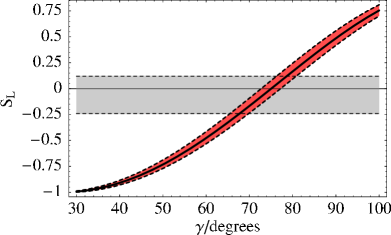
Figure 2: Theoretical result for the longitudinal time-dependent CP-asymmetry parameter $S_{L}^{{\rho}{\rho}}$ as a function of the CKM angle $\gamma$. The horizontal band indicates the current experimental constraint [44, 49].

Figure 2 shows $S_{L}^{{\rho}{\rho}}$ as a function of $\gamma$ in the range of interest. The band quantifies the theoretical uncertainty. From the intersection of this band with the measured value $-0.06\pm 0.18$ [44, 49], and given $\beta=(21.2\pm 1.0)^{\circ}$ [50, 51, 52], we obtain

$$\gamma=(73.2^{+7.6}_{-7.7})^{\circ}\qquad\mbox{or}\qquad\alpha=(85.6^{+7.4}_{-7.3})^{\circ},$$ (34)

where the theoretical error alone is only $\pm 3^{\circ}$. The value of $\gamma$ obtained in this way is remarkably consistent with the one from QCD factorisation calculations of the $S$-parameters of the $\pi^{+}\pi^{-}$ and $\pi^{\pm}\rho^{\mp}$ final states [25, 53], and presently provides the most accurate direct determination of $\gamma$. It is also consistent with [54], where instead of a theoretical calculation of $P/T$ one uses SU(3) symmetry to relate the penguin amplitude to the longitudinal branching fraction of ${B}^{-}\to\rho^{-}\bar{K}^{*0}$, and with other determinations of $\gamma$ ($\alpha$) from $B\to\rho\rho$ decays [44, 49].

5.3 Polarisation observables

We now study the transverse-helicity contributions, which manifest themselves in polarisation observables. As explained before, model-dependent effects such as non-factorisation of spectator-scattering and penguin annihilation can make a strong impact on transverse amplitudes, and therefore our results suffer from larger uncertainties. Here, this specifically concerns the five colour-suppressed modes. On the other hand, as polarisation observables like $f_{L}$ involve ratios, other uncertainties are often reduced. Specifically, CKM factors often drop out approximately, and form factors only enter in form of ratios (for example transverse/longitudinal), when only one form factor contribution is present or strongly dominant in an amplitude.

	$f_{L}$ / percent			$A_{\mathrm{CP}}^{0}$ / percent
	Theory	Experiment		Theory
${B}^{-}\to{\rho}^{-}{\rho}^{0}$	$95.9^{+0.2}_{-0.3}{}^{+3.4}_{-5.9}$	$91.2^{+4.4}_{-4.5}$		$-0^{+0}_{-0}{}^{+0}_{-0}$
$\bar{{B}}^{0}\to{\rho}^{+}{\rho}^{-}$	$91.3^{+0.4}_{-0.3}{}^{+5.6}_{-6.4}$	$96.8\pm 2.3$		$-2^{+0}_{-0}{}^{+4}_{-2}$
$\bar{{B}}^{0}\to{\rho}^{0}{\rho}^{0}$	$90^{+3}_{-4}{}^{+8}_{-56}$	$87\pm 14$		$-8^{+2}_{-1}{}^{+59}_{-28}$
${B}^{-}\to{\omega}{\rho}^{-}$	$93.7^{+1.1}_{-1.0}{}^{+4.7}_{-8.1}$	$82\pm 11$		$-2^{+1}_{-0}{}^{+7}_{-6}$
$\bar{{B}}^{0}\to{\omega}{\rho}^{0}$	$49^{+11}_{-11}{}^{+47}_{-23}$	n/a		$+35^{+25}_{-15}{}^{+47}_{-84}$
$\bar{{B}}^{0}\to{\omega}{\omega}$	$93^{+2}_{-4}{}^{+5}_{-22}$	n/a		$+6^{+1}_{-1}{}^{+14}_{-24}$
$\bar{{B}}_{s}\to{K}^{*+}\rho^{-}$	$92.2^{+0.6}_{-0.5}{}^{+5.2}_{-7.5}$	n/a		$-2^{+1}_{-0}{}^{+6}_{-3}$
$\bar{{B}}_{s}\to{K}^{*0}\rho^{0}$	$93^{+2}_{-3}{}^{+5}_{-54}$	n/a		$-5^{+1}_{-0}{}^{+49}_{-18}$
$\bar{{B}}_{s}\to{K}^{*0}\omega$	$93^{+2}_{-4}{}^{+5}_{-49}$	n/a		$+6^{+1}_{-1}{}^{+19}_{-60}$

Table 5: Longitudinal polarisation fraction and the corresponding CP asymmetry for tree-dominated decays. Experimental values are taken from [42, 43, 44, 45, 46, 47].

Our results for the longitudinal polarisation fraction and the corresponding CP asymmetry are shown in Table 5. As expected the colour-allowed tree-dominated decay modes are predicted to have $f_{L}$ near 1 with errors in the $(5-10)\%$ range. Their longitudinal CP asymmetries are predicted not to exceed $10\%$. Again the situation is very different for the colour-suppressed decays. With the exception of $\bar{{B}}^{0}\to{\omega}{\rho}^{0}$ there is still a preference for significant longitudinal polarisation, but much smaller values can be obtained within theoretical errors. The large downward uncertainty is entirely due to the model-dependence in the spectator-scattering contribution to the negative helicity amplitude $\alpha_{2}^{-}$ (parameterised by $X_{H}$ in the QCD factorisation formalism). The longitudinal CP asymmetries are also very uncertain.

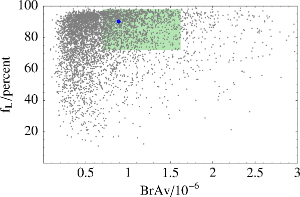
Figure 3: Correlation of branching fraction and longitudinal polarisation fraction in $\bar{{B}}^{0}\to{\rho}^{0}{\rho}^{0}$, illustrated using 5000 randomly chosen points in our parameter space. The shaded area corresponds to the BABAR measurement [45], the highlighted point to our default values.

The theoretical predictions of $f_{L}$ are compatible with the present experimental data where available. One notices, however, that the pattern of $1-f_{L}$ for the two colour-allowed $\rho\rho$ final states seen by experiment appears to be opposite to the theoretical one though perhaps not significantly. We therefore calculate

$$r_{+0}=\frac{1-f_{L}(\rho^{-}\rho^{0})}{1-f_{L}(\rho^{+}\rho^{-})}=0.46^{+0.06}_{-0.04}{}^{+1.63}_{-0.42}\qquad\mbox{(exp: }2.75^{+2.43}_{-2.41}).$$ (35)

The theoretical upper limit of $r_{+0}\approx 2$ is attained when spectator-scattering is minimal ($X_{H}=-1$), in which case $f_{L}(\rho^{-}\rho^{0})\approx 0.90$ and $f_{L}(\rho^{+}\rho^{-})\approx 0.95$. The branching fraction and longitudinal polarisation fraction of the colour-suppressed decay $\bar{{B}}^{0}\to\rho^{0}\rho^{0}$ are theoretically allowed to lie within large ranges. To investigate the question whether there exist (theoretical) correlations between the two observables, we perform a random scan through the theory parameter space. The result is displayed in Figure 3. It shows that while there is a preference for smaller branching fractions than in our default prediction, there is no obvious correlation between the branching fraction and $f_{L}$.

The remaining six polarisation observables can be taken to be $f_{\parallel}-f_{\perp}$, $A_{\rm CP}^{\parallel}-A_{\rm CP}^{\perp}$, and the phase differences between the transverse helicity amplitudes and the longitudinal amplitude. As explained in Section 3, $f_{\perp}$, $A^{\perp}_{\rm CP}$, $\phi_{\perp}$, $\Delta\phi_{\perp}$ are expected to be approximately equal to $f_{\parallel}$, $A^{\parallel}_{\rm CP}$, $\phi_{\parallel}$, $\Delta\phi_{\parallel}$. We find indeed that $f_{\parallel}-f_{\perp}$ is always below $2\%$. The last column of Table 6 quantifies the expectation of equal $\phi_{\parallel}$ and $\phi_{\perp}$: the difference of the two does not exceed a few degrees. We should point out, however, that this calculation relies on the assumption that the positive-helicity is not substantially different from its magnitude in naive factorisation. In view of this the smallness of $\phi_{\parallel}-\phi_{\perp}$ should be interpreted as the statement that no concrete dynamical mechanism is known that could produce a larger difference. The phase observables $\phi_{\parallel}$ and the corresponding CP asymmetry $\Delta\phi_{\parallel}$ are shown in the second and third column of Table 6. For most of the colour-suppressed decays the theoretical uncertainty is above $270^{\circ}$, in which case we conclude that no useful theoretical prediction is possible. For the colour-allowed modes, we obtain reasonably accurate results, which could be compared to experiment, once a complete angular analysis is performed.

	$\phi_{\parallel}$ / degrees	$\Delta\phi_{\parallel}$ / degrees	$(\phi_{\parallel}-\phi_{\perp})$ / degrees
${B}^{-}\to{\rho}^{-}{\rho}^{0}$	$-5^{+0}_{-0}{}^{+31}_{-32}$	$-6^{+2}_{-1}{}^{+2}_{-5}$	$\pm 2$
$\bar{{B}}^{0}\to{\rho}^{+}{\rho}^{-}$	$+1^{+2}_{-2}{}^{+17}_{-17}$	$+4^{+1}_{-1}{}^{+9}_{-9}$	$\pm 0$
$\bar{{B}}^{0}\to{\rho}^{0}{\rho}^{0}$	no prediction	no prediction	$\pm 3$
${B}^{-}\to{\omega}{\rho}^{-}$	$-9^{+2}_{-2}{}^{+34}_{-28}$	$+18^{+6}_{-6}{}^{+34}_{-31}$	$\pm 3$
$\bar{{B}}^{0}\to{\omega}{\rho}^{0}$	$-29^{+5}_{-4}{}^{+58}_{-58}$	$-45^{+13}_{-17}{}^{+61}_{-37}$	$\pm 1$
$\bar{{B}}^{0}\to{\omega}{\omega}$	no prediction	no prediction	$\pm 3$
$\bar{{B}}_{s}\to{K}^{*+}\rho^{-}$	$-1^{+3}_{-2}{}^{+21}_{-21}$	$+7^{+2}_{-2}{}^{+13}_{-14}$	$\pm 0$
$\bar{{B}}_{s}\to{K}^{*0}\rho^{0}$	no prediction	no prediction	$\pm 2$
$\bar{{B}}_{s}\to{K}^{*0}\omega$	no prediction	no prediction	$\pm 3$

Table 6: Predictions for other polarisation observables

6 Penguin-dominated decays

The 14 decay modes that we study in this section are characterised by the dominant role of the colour-allowed QCD penguin amplitude $\hat{\alpha}_{4}^{p}\equiv\alpha_{4}^{p}+\beta_{3}^{p}$, which includes a penguin-annihilation term. Of these the 11 $\Delta S=1$ modes have branching fractions up to $10^{5}$, and some of them have already been studied extensively experimentally including polarisation.

Due to their common dominant amplitude the theoretical errors in this class of decays are common to all representatives. As explained in Section 3.2, the negative-helicity penguin amplitude $\hat{\alpha}_{4}^{p-}$ is particularly uncertain due to a potentially large penguin weak annihilation contribution [6]. In addition, non-factorisation of spectator scattering also affects the transverse amplitude of final states containing $\omega$ or $\phi$ mesons, mostly through the flavour-singlet penguin amplitude $\alpha_{3}^{p-}$. An important issue of the subsequent analysis will be whether theoretical calculations are compatible with the observation of large transverse polarisation, and whether uncertainties can be controlled to the point that useful predictions can be made.

6.1 The ${B}\to{\phi}{K}^{*}$ system and the transverse penguin amplitude

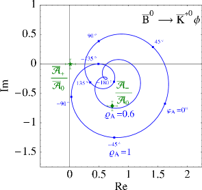
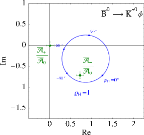
Figure 4: Transverse-to-longitudinal amplitude ratios for $\bar{{B}}^{0}\to\bar{{K}}^{*}\phi$. The contours indicate the dependence of the negative-helicity theory prediction on annihilation (left) and spectator scattering (right) parameters, with all other input fixed at central values. Additionally, the values implied by current measurements [26, 27, 29] for both helicities are shown.

We begin with a discussion of the ${B}\to{\phi}{K}^{*}$ modes. A complete angular analysis is available for ${B}\to{\phi}{K}^{*0}$ [26, 29], which allows us to extract the complex amplitude ratios $\bar{}\mathcal{A}_{\pm}/\bar{}\mathcal{A}_{0}$ from data. This is shown in Figure 4, which compares this result to the theoretical calculation of $\bar{}\mathcal{A}_{-}/\bar{}\mathcal{A}_{0}$. (The experimental result for $\bar{}\mathcal{A}_{+}/\bar{}\mathcal{A}_{0}$ is in very good agreement with the expectation that the plus-helicity amplitude should be strongly suppressed.) The left plot in the figure shows the theoretical range from a variation of the uncertainties in weak annihilation alone (parameter $X_{A}$), the right plot displays the same information for spectator scattering (parameter $X_{H}$). Since all values for inside the contour are theoretically allowed for $\bar{\mathcal{A}}_{-}/\bar{\mathcal{A}}_{0}$, it is evident that theory does not require the amplitude ratio to be small. While it does not make accurate predictions, it is natural that penguin-dominated decays exhibit large transverse polarisation. This is confirmed by comparing the first column of numbers in Table 7 with the measurements in the fourth column. We find very good agreement of our results with data but with very large uncertainties. We also note that all observables related to the positive-helicity amplitude (the difference of $\parallel$ and $\perp$ observables) are predicted to be very small. So are the CP asymmetries, since the doubly CKM-suppressed amplitude proportional to $\lambda_{u}^{(s)}$ does not exceed a few percent. Unless experiments find unexpectedly large values for any of these observables, the interesting ones are the branching fraction, $f_{L}$ and the phase $\phi_{\parallel}$.

Observable		Theory			Experiment
		default	constrained $X_{A}$	$\hat{\alpha}_{4}^{c-}$ from data
$\operatorname{BrAv}/10^{-6}$	${\phi}{K}^{*-}$	$10.1^{+0.5}_{-0.5}{}^{+12.2}_{-7.1}$	$10.1^{+0.5}_{-0.5}{}^{+7.2}_{-4.8}$	$10.4^{+0.5}_{-0.5}{}^{+5.2}_{-3.9}$	$9.7\pm 1.5$
	${\phi}\bar{{K}}^{*0}$	$\phantom{1}9.3^{+0.5}_{-0.5}{}^{+11.4}_{-6.5}$	$\phantom{1}9.3^{+0.5}_{-0.5}{}^{+6.7}_{-4.5}$	$\phantom{1}9.6^{+0.5}_{-0.5}{}^{+4.7}_{-3.6}$	$9.5\pm 0.8$
$A_{\mathrm{CP}}/\%$	${\phi}{K}^{*-}$	$0^{+0}_{-0}{}^{+2}_{-1}$	$0^{+0}_{-0}{}^{+0}_{-0}$	$0^{+0}_{-0}{}^{+3}_{-2}$	$5\pm 11$
	${\phi}\bar{{K}}^{*0}$	$1^{+0}_{-0}{}^{+1}_{-0}$	$1^{+0}_{-0}{}^{+0}_{-0}$	$1^{+0}_{-0}{}^{+2}_{-1}$	$-1\pm 6$
$f_{L}/\%$	${\phi}{K}^{*-}$	$45^{+0}_{-0}{}^{+58}_{-36}$	$45^{+0}_{-0}{}^{+35}_{-31}$	$44^{+0}_{-0}{}^{+23}_{-23}$	$50\pm 7$
	${\phi}\bar{{K}}^{*0}$	$44^{+0}_{-0}{}^{+59}_{-36}$	$44^{+0}_{-0}{}^{+35}_{-31}$	$43^{+0}_{-0}{}^{+23}_{-23}$	$49\pm 3$
$A_{\mathrm{CP}}^{0}/\%$	${\phi}{K}^{*-}$	$-1^{+0}_{-0}{}^{+2}_{-1}$	$-1^{+0}_{-0}{}^{+1}_{-1}$	$-1^{+0}_{-0}{}^{+2}_{-2}$	n/a
	${\phi}\bar{{K}}^{*0}$	$\phantom{-}0^{+0}_{-0}{}^{+1}_{-1}$	$\phantom{-}0^{+0}_{-0}{}^{+1}_{-0}$	$\phantom{-}0^{+0}_{-0}{}^{+1}_{-2}$	$2\pm 7$
$(f_{\parallel}-f_{\perp})/\%$	${\phi}{K}^{*-}$	$0^{+0}_{-0}{}^{+2}_{-2}$	$0^{+0}_{-0}{}^{+2}_{-2}$	$0^{+0}_{-0}{}^{+2}_{-2}$	$12\pm 17$
	${\phi}\bar{{K}}^{*0}$	$0^{+0}_{-0}{}^{+2}_{-2}$	$0^{+0}_{-0}{}^{+2}_{-2}$	$0^{+0}_{-0}{}^{+2}_{-2}$	$1\pm 7$
$(A_{\mathrm{CP}}^{\parallel}-A_{\mathrm{CP}}^{\perp})/\%$	${\phi}{K}^{*-}$	$0^{+0}_{-0}{}^{+0}_{-0}$	$0^{+0}_{-0}{}^{+0}_{-0}$	$0^{+0}_{-0}{}^{+0}_{-0}$	n/a
	${\phi}\bar{{K}}^{*0}$	$0^{+0}_{-0}{}^{+0}_{-0}$	$0^{+0}_{-0}{}^{+0}_{-0}$	$0^{+0}_{-0}{}^{+0}_{-0}$	$18\pm 28$
$\phi_{\parallel}/^{\circ}$	${\phi}{K}^{*-}$	$-41^{+0}_{-0}{}^{+84}_{-53}$	$-41^{+0}_{-0}{}^{+35}_{-30}$	$-40^{+0}_{-0}{}^{+21}_{-21}$	$-60\pm 16$
	${\phi}\bar{{K}}^{*0}$	$-42^{+0}_{-0}{}^{+87}_{-54}$	$-42^{+0}_{-0}{}^{+35}_{-30}$	$-42^{+0}_{-0}{}^{+21}_{-21}$	$-44\pm 8$
$\Delta\phi_{\parallel}/^{\circ}$	${\phi}{K}^{*-}$	$0^{+0}_{-0}{}^{+0}_{-1}$	$0^{+0}_{-0}{}^{+0}_{-0}$	$0^{+0}_{-0}{}^{+0}_{-0}$	n/a
	${\phi}\bar{{K}}^{*0}$	$0^{+0}_{-0}{}^{+0}_{-0}$	$0^{+0}_{-0}{}^{+0}_{-0}$	$0^{+0}_{-0}{}^{+0}_{-1}$	$6\pm 8$
$(\phi_{\parallel}-\phi_{\perp})/^{\circ}$	${\phi}{K}^{*-}$	$0^{+0}_{-0}{}^{+1}_{-1}$	$0^{+0}_{-0}{}^{+1}_{-1}$	$0^{+0}_{-0}{}^{+1}_{-1}$	$-12\pm 24$
	${\phi}\bar{{K}}^{*0}$	$0^{+0}_{-0}{}^{+1}_{-1}$	$0^{+0}_{-0}{}^{+1}_{-1}$	$0^{+0}_{-0}{}^{+1}_{-1}$	$1\pm 11$
$(\Delta\phi_{\parallel}-\Delta\phi_{\perp})/^{\circ}$	${\phi}{K}^{*-}$	$0^{+0}_{-0}{}^{+0}_{-0}$	$0^{+0}_{-0}{}^{+0}_{-0}$	$0^{+0}_{-0}{}^{+0}_{-0}$	n/a
	${\phi}\bar{{K}}^{*0}$	$0^{+0}_{-0}{}^{+0}_{-0}$	$0^{+0}_{-0}{}^{+0}_{-0}$	$0^{+0}_{-0}{}^{+0}_{-0}$	$3\pm 11$

Table 7: Comparison of theoretical results for observables from the full angular analysis of ${B}^{-}\to{\phi}{K}^{*-}$ and $\bar{{B}}^{0}\to{\phi}\bar{{K}}^{*0}$ with experimental results from [26, 27, 29].

We now explore a strategy where the variation of input parameters or the transverse penguin amplitude $\hat{\alpha}_{4}^{p-}$ is constrained by data in order to improve the predictions for other observables and decay modes. We assume that this amplitude is approximately the same for all decay modes, in accordance with factorisation calculations. Figure 4 allows explanations for the large negative-helicity amplitude based on spectator scattering or weak annihilation (or both). We favour the second option, since an enhancement of spectator scattering would lead to large transverse polarisation for the colour-suppressed tree decays which is not observed for the $\rho^{0}\rho^{0}$ final state, see Section 5. Further support for this option comes from the $\rho{K}^{*}$ final states, which do not involve $\alpha_{3}^{p}$, and which are therefore much less sensitive to spectator scattering. Figure 5 displays three observables from the $\rho{K}^{*}$ system as a function of the strength of weak annihilation, $\varrho_{A}$. It can be seen that it must be non-zero, with a favoured range around $\varrho_{A}\approx 0.6$. This is consistent with a fit of $\varrho_{A}\,e^{i\varphi_{A}}$ to the ${\phi}{K}^{*0}$ data, which suggests

$$\varrho_{A}=0.5\pm 0.2_{\text{exp.}}\qquad\varphi_{A}=(-43\pm 19_{\text{exp.}})^{\circ},$$ (36)

excluding other theory uncertainties. This coincidence motivates the default input parameter choice $\varrho_{A}\,e^{i\varphi_{A}}=0.6\,e^{-i40^{\circ}}$ adopted in Section 4. The second column in Table 7 shows the theoretical prediction when the variation of these parameters is reduced to $\varrho_{A}=0.6\pm 0.2$ and $\varphi_{A}=(-40\pm 10)^{\circ}$ as suggested by (36) and Figure 5. The central values of these results remain the same by construction, but the hadronic uncertainties are considerably reduced.

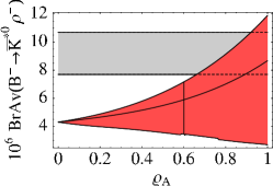
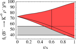
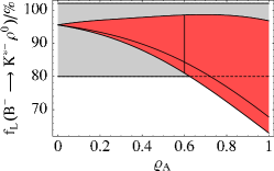
Figure 5: Predicted branching fraction and longitudinal polarisation fraction of the pure penguin decay ${B}^{-}\to\bar{{K}}^{*0}{\rho}^{-}$ (left and center) and longitudinal polarisation fraction of ${B}^{-}\to{K}^{*-}{\rho}^{0}$ (right) as a function of the parameter $\varrho_{A}$ of our annihilation model, showing only the theory uncertainty from variation of the phase $\varphi_{A}$. The horizontal band represents current experimental values [50]. The lines within the theory band indicate our default choices for $\varrho_{A}$ and $\varphi_{A}$.

Rather than relying on our model-dependent parameterisation of the weak annihilation amplitude to fit data, we prefer the point of view that $\hat{\alpha}_{4}^{p-}$ is theoretically unreliable and should be taken from data. Thus, instead of $\varrho_{A}\,e^{i\varphi_{A}}$ we fit $\hat{\alpha}_{4}^{p-}$. Neglecting CP violation in the $\phi{K}^{*}$ system in accordance with the present data and theoretical expectations, the transverse amplitude can be expressed as

$$\bar{\mathcal{A}}_{-}=A_{\bar{{K}}^{*}\phi}\lambda^{(s)}_{c}P^{\bar{{K}}^{*}\phi}_{-},$$ (37)

where, neglecting small coefficients, $P^{\bar{{K}}^{*}\phi}_{-}\approx\hat{\alpha}_{4}^{c-}(\bar{{K}}^{*}\phi)+\alpha_{3}^{c}(\bar{{K}}^{*}\phi)$. Calculating $\bar{\mathcal{A}}_{-}$ from the data with the overall phase adapted so that the phases of the longitudinal helicity amplitudes from theory and data match, we obtain

$$P^{\bar{{K}}^{*}\phi}_{-}=(-0.081\pm 0.002\text{(exp)}{}^{+0.008}_{-0.009}\text{(th)})+i\,(0.026\pm 0.011\text{(exp)}{}^{+0.003}_{-0.003}\text{(th)}),$$ (38)

where the theoretical error includes the uncertainties from $A_{\bar{{K}}^{*}\phi}\lambda^{(s)}_{c}$ only. Since we already assumed that a large enhancement of $\alpha_{3}^{c-}$ is not a favoured option, we obtain $\hat{\alpha}_{4}^{c-}$ by subtracting the default value of $\alpha_{3}^{c-}$. Rounding numbers, this results in

$$\hat{\alpha}_{4}^{c-}=(-0.08\pm 0.02)+i\,(0.03\pm 0.02).$$ (39)

This is the input to the theoretical predictions shown in the third column of Table 7 and the columns labeled “$\hat{\alpha}_{4}^{c-}$ from data” in later tables in this section. This procedure provides another considerable reduction of hadronic uncertainties.

6.2 Branching fractions, direct CP asymmetries and polarisation

We now discuss the complete set of final states, where the $\hat{\alpha}_{4}^{c}$ amplitude is dominant. The CP-averaged branching fractions, direct CP asymmetries and longitudinal polarisation fractions are given in Tables 8, 9 and 10, respectively. The two columns of numbers in these tables represent the result with our default inputs with uncertainties, and the result using (39) as input. In general, we regard the second result as our “best” prediction. However, one should be aware that it depends on the assumption of final-state independence of $\hat{\alpha}_{4}^{c}$, and the present experimental data.

$\operatorname{BrAv}/10^{-6}$	Theory		Experiment
	default	$\hat{\alpha}_{4}^{c-}$ from data
${B}^{-}\to{K}^{*-}{\phi}$	$10.1^{+0.5}_{-0.5}{}^{+12.2}_{-7.1}$	$10.4^{+0.5}_{-0.5}{}^{+5.2}_{-3.9}$	$9.7\pm 1.5$
$\bar{{B}}^{0}\to\bar{{K}}^{*0}{\phi}$	$9.3^{+0.5}_{-0.5}{}^{+11.4}_{-6.5}$	$9.6^{+0.5}_{-0.5}{}^{+4.7}_{-3.6}$	$9.5\pm 0.8$
${B}^{-}\to{K}^{*-}{\omega}$	$2.4^{+0.8}_{-0.7}{}^{+2.9}_{-1.3}$	$2.3^{+0.8}_{-0.7}{}^{+1.4}_{-0.7}$	$<3.4$
$\bar{{B}}^{0}\to\bar{{K}}^{*0}{\omega}$	$2.0^{+0.1}_{-0.1}{}^{+3.1}_{-1.4}$	$1.9^{+0.1}_{-0.1}{}^{+1.5}_{-0.7}$	$<4.2$
${B}^{-}\to\bar{{K}}^{*0}{\rho}^{-}$	$5.9^{+0.3}_{-0.3}{}^{+6.9}_{-3.7}$	$5.8^{+0.3}_{-0.3}{}^{+3.1}_{-1.9}$	$9.2\pm 1.5$
${B}^{-}\to{K}^{*-}{\rho}^{0}$	$4.5^{+1.5}_{-1.3}{}^{+3.0}_{-1.4}$	$4.5^{+1.5}_{-1.3}{}^{+1.8}_{-1.0}$	$<6.1$
$\bar{{B}}^{0}\to{K}^{*-}{\rho}^{+}$	$5.5^{+1.7}_{-1.5}{}^{+5.7}_{-2.9}$	$5.4^{+1.7}_{-1.5}{}^{+2.6}_{-1.5}$	$<12$
$\bar{{B}}^{0}\to\bar{{K}}^{*0}{\rho}^{0}$	$2.4^{+0.2}_{-0.1}{}^{+3.5}_{-2.0}$	$2.3^{+0.2}_{-0.1}{}^{+1.1}_{-0.8}$	$5.6\pm 1.6$
$\bar{{B}}_{s}\to{K}^{*-}{K}^{*+}$	$9.1^{+2.5}_{-2.2}{}^{+10.2}_{-5.9}$	$8.0^{+2.4}_{-2.1}{}^{+3.7}_{-3.4}$	n/a
$\bar{{B}}_{s}\to{K}^{*0}\bar{{K}}^{*0}$	$9.1^{+0.5}_{-0.4}{}^{+11.3}_{-6.8}$	$7.9^{+0.4}_{-0.4}{}^{+4.3}_{-3.9}$	n/a
$\bar{{B}}_{s}\to{\phi}{\phi}$	$21.8^{+1.1}_{-1.1}{}^{+30.4}_{-17.0}$	$19.5^{+1.0}_{-1.0}{}^{+13.1}_{-8.0}$	$14.0^{+8.0}_{-7.0}$
${B}^{-}\to{K}^{*0}{K}^{*-}$	$0.5^{+0.2}_{-0.1}{}^{+0.4}_{-0.3}$	$0.5^{+0.2}_{-0.1}{}^{+0.2}_{-0.2}$	$<71$
$\bar{{B}}^{0}\to{K}^{*0}\bar{{K}}^{*0}$	$0.6^{+0.1}_{-0.1}{}^{+0.5}_{-0.3}$	$0.6^{+0.1}_{-0.1}{}^{+0.3}_{-0.2}$	$<22$
$\bar{{B}}_{s}\to{K}^{*0}{\phi}$	$0.4^{+0.1}_{-0.1}{}^{+0.5}_{-0.3}$	$0.3^{+0.1}_{-0.1}{}^{+0.2}_{-0.1}$	n/a

Table 8: CP-averaged branching fractions of $\Delta S=1$ and $\Delta D=1$ penguin-dominated $B\to VV$ decays. Experimental values are taken from [26, 27, 29, 42, 55, 56, 57].

The two ${\omega}{K}^{*}$ modes are predicted to have 4–5 times smaller branching fractions than the ${\phi}{K}^{*}$ modes, which is consistent with experimental upper limits. Following the notation of the appendix of [25] and suppressing helicity labels $h$, the decay amplitudes read

$$\sqrt{2}\mathcal{A}_{{B}^{-}\to{\omega}{K}^{*-}} =A_{\bar{{K}}^{*}{\omega}}\left[2\alpha_{3}^{p}+\delta_{pu}\,\alpha_{2}\right]+A_{{\omega}\bar{{K}}^{*}}\left[\hat{\alpha}_{4}^{p}+\delta_{pu}\,\alpha_{1}\right],$$ (40)

$$\sqrt{2}\mathcal{A}_{\bar{{B}}^{0}\to{\omega}\bar{{K}}^{*0}} =A_{\bar{{K}}^{*}{\omega}}\left[2\alpha_{3}^{p}+\delta_{pu}\,\alpha_{2}\right]+A_{{\omega}\bar{{K}}^{*}}\hat{\alpha}_{4}^{p},$$

where we do not show numerically irrelevant amplitudes. The smaller branching fraction is simply a consequence of a relative factor of $\sqrt{2}$ in the amplitude, and the smaller $B\to\omega$ form factors multiplying the dominant $\hat{\alpha}_{4}^{c}$ coefficient ($|A_{\bar{{K}}^{*}{\phi}}^{0,-}/A_{\omega\bar{{K}}^{*}}^{0,-}|^{2}\approx 2.5$). As both factors cancel out in the polarisation fraction, $f_{L}$ is predicted to be similar for $\omega K^{*}$ and ${\phi}{K}^{*}$. However, contrary to the $\phi{K}^{*}$ system, the presence of tree amplitudes $\alpha_{1,2}$ in (40) allows for sizeable CP asymmetries as can be seen from Table 9.

$A_{\mathrm{CP}}$ / percent	Theory		Experiment
	default	$\hat{\alpha}_{4}^{c-}$ from data
${B}^{-}\to{K}^{*-}{\phi}$	$\phantom{1}0^{+0}_{-0}{}^{+2}_{-1}$	$\phantom{1}0^{+0}_{-0}{}^{+3}_{-2}$	$5\pm 11$
$\bar{{B}}^{0}\to\bar{{K}}^{*0}{\phi}$	$\phantom{1}1^{+0}_{-0}{}^{+1}_{-0}$	$\phantom{1}1^{+0}_{-0}{}^{+2}_{-1}$	$1\pm 6$
${B}^{-}\to{K}^{*-}{\omega}$	$22^{+4}_{-5}{}^{+40}_{-21}$	$24^{+5}_{-6}{}^{+25}_{-24}$	n/a
$\bar{{B}}^{0}\to\bar{{K}}^{*0}{\omega}$	$19^{+5}_{-4}{}^{+17}_{-16}$	$20^{+6}_{-5}{}^{+16}_{-15}$	n/a
${B}^{-}\to\bar{{K}}^{*0}{\rho}^{-}$	$\phantom{1}0^{+0}_{-0}{}^{+3}_{-1}$	$\phantom{1}0^{+0}_{-0}{}^{+3}_{-2}$	$-1\pm 16$
${B}^{-}\to{K}^{*-}{\rho}^{0}$	$16^{+4}_{-4}{}^{+23}_{-16}$	$16^{+4}_{-4}{}^{+17}_{-14}$	$20^{+32}_{-29}$
$\bar{{B}}^{0}\to{K}^{*-}{\rho}^{+}$	$\phantom{1}5^{+1}_{-1}{}^{+40}_{-17}$	$\phantom{1}6^{+2}_{-2}{}^{+16}_{-12}$	n/a
$\bar{{B}}^{0}\to\bar{{K}}^{*0}{\rho}^{0}$	$-15^{+4}_{-4}{}^{+17}_{-32}$	$-15^{+4}_{-4}{}^{+16}_{-16}$	$9\pm 19$
$\bar{{B}}_{s}\to{K}^{*-}{K}^{*+}$	$\phantom{1}2^{+0}_{-0}{}^{+40}_{-15}$	$\phantom{1}4^{+1}_{-1}{}^{+20}_{-12}$	n/a
$\bar{{B}}_{s}\to{K}^{*0}\bar{{K}}^{*0}$	$\phantom{1}1^{+0}_{-0}{}^{+1}_{-0}$	$\phantom{1}1^{+0}_{-0}{}^{+2}_{-1}$	n/a
$\bar{{B}}_{s}\to{\phi}{\phi}$	$\phantom{1}1^{+0}_{-0}{}^{+1}_{-0}$	$\phantom{1}1^{+0}_{-0}{}^{+2}_{-1}$	n/a
${B}^{-}\to{K}^{*0}{K}^{*-}$	$\phantom{1}0^{+0}_{-0}{}^{+17}_{-40}$	$\phantom{1}1^{+0}_{-0}{}^{+30}_{-55}$	n/a
$\bar{{B}}^{0}\to{K}^{*0}\bar{{K}}^{*0}$	$-13^{+3}_{-4}{}^{+6}_{-8}$	$-13^{+3}_{-4}{}^{+17}_{-24}$	n/a
$\bar{{B}}_{s}\to{K}^{*0}{\phi}$	$-17^{+4}_{-5}{}^{+9}_{-9}$	$-16^{+4}_{-4}{}^{+31}_{-51}$	n/a

Table 9: Direct CP asymmetries of $\Delta S=1$ and $\Delta D=1$ penguin-dominated $B\to VV$ decays. Experimental values are taken from [26, 27, 29, 42, 55].

$f_{L}$ / percent	Theory		Experiment
	default	$\hat{\alpha}_{4}^{c-}$ from data
${B}^{-}\to{K}^{*-}{\phi}$	$45^{+0}_{-0}{}^{+58}_{-36}$	$44^{+0}_{-0}{}^{+23}_{-23}$	$50.0\pm 7.0$
$\bar{{B}}^{0}\to\bar{{K}}^{*0}{\phi}$	$44^{+0}_{-0}{}^{+59}_{-36}$	$43^{+0}_{-0}{}^{+23}_{-23}$	$49.1\pm 3.2$
${B}^{-}\to{K}^{*-}{\omega}$	$53^{+8}_{-11}{}^{+57}_{-39}$	$56^{+8}_{-11}{}^{+22}_{-19}$	n/a
$\bar{{B}}^{0}\to\bar{{K}}^{*0}{\omega}$	$40^{+4}_{-3}{}^{+77}_{-43}$	$43^{+4}_{-3}{}^{+38}_{-32}$	n/a
${B}^{-}\to\bar{{K}}^{*0}{\rho}^{-}$	$56^{+0}_{-0}{}^{+48}_{-30}$	$57^{+0}_{-0}{}^{+21}_{-18}$	$48.0\pm 8.0$
${B}^{-}\to{K}^{*-}{\rho}^{0}$	$84^{+2}_{-3}{}^{+16}_{-25}$	$85^{+2}_{-3}{}^{+9}_{-11}$	$96^{+6}_{-16}$
$\bar{{B}}^{0}\to{K}^{*-}{\rho}^{+}$	$61^{+5}_{-7}{}^{+38}_{-28}$	$62^{+5}_{-6}{}^{+17}_{-15}$	n/a
$\bar{{B}}^{0}\to\bar{{K}}^{*0}{\rho}^{0}$	$22^{+3}_{-3}{}^{+53}_{-14}$	$22^{+3}_{-3}{}^{+21}_{-13}$	$57\pm 12$
$\bar{{B}}_{s}\to{K}^{*-}{K}^{*+}$	$67^{+4}_{-5}{}^{+31}_{-26}$	$76^{+3}_{-4}{}^{+12}_{-16}$	n/a
$\bar{{B}}_{s}\to{K}^{*0}\bar{{K}}^{*0}$	$63^{+0}_{-0}{}^{+42}_{-29}$	$72^{+0}_{-0}{}^{+16}_{-21}$	n/a
$\bar{{B}}_{s}\to{\phi}{\phi}$	$43^{+0}_{-0}{}^{+61}_{-34}$	$48^{+0}_{-0}{}^{+26}_{-27}$	n/a
${B}^{-}\to{K}^{*0}{K}^{*-}$	$62^{+1}_{-2}{}^{+42}_{-33}$	$62^{+1}_{-2}{}^{+18}_{-19}$	n/a
$\bar{{B}}^{0}\to{K}^{*0}\bar{{K}}^{*0}$	$69^{+1}_{-1}{}^{+34}_{-27}$	$69^{+1}_{-1}{}^{+16}_{-20}$	n/a
$\bar{{B}}_{s}\to{K}^{*0}{\phi}$	$40^{+1}_{-1}{}^{+67}_{-35}$	$47^{+3}_{-2}{}^{+28}_{-24}$	n/a

Table 10: Longitudinal polarisation fraction of $\Delta S=1$ and $\Delta D=1$ penguin-dominated $B\to VV$ decays. Experimental values are taken from [26, 27, 29, 42, 55, 56].

The four ${K}^{*}{\rho}$ final states are the $VV$ equivalents to the much discussed $\pi K$ final states. Their amplitudes are given by

$$\mathcal{A}_{{B}^{-}\to{\rho}^{-}\bar{{K}}^{*0}} =A_{\rho\bar{{K}}^{*}}\,\hat{\alpha}_{4}^{p},$$ (41)

$$\sqrt{2}\,\mathcal{A}_{{B}^{-}\to{\rho}^{0}{K}^{*-}} =A_{\rho\bar{{K}}^{*}}\big{[}\hat{\alpha}_{4}^{p}+\delta_{pu}\alpha_{1}\big{]}+A_{\bar{{K}}^{*}\rho}\left[\frac{3}{2}\alpha_{3,\mathrm{EW}}^{p}+\delta_{pu}\alpha_{2}\right],$$

$$\mathcal{A}_{\bar{{B}}^{0}\to{\rho}^{+}{K}^{*-}} =A_{\rho\bar{{K}}^{*}}\big{[}\hat{\alpha}_{4}^{p}+\delta_{pu}\alpha_{1}\big{]},$$

$$-\sqrt{2}\,\mathcal{A}_{\bar{{B}}^{0}\to{\rho}^{0}\bar{{K}}^{*0}} =A_{\rho\bar{{K}}^{*}}\,\hat{\alpha}_{4}^{p}-A_{\bar{{K}}^{*}\rho}\left[\frac{3}{2}\alpha_{3,\mathrm{EW}}^{p}+\delta_{pu}\alpha_{2}\right].$$

They are particularly interesting, because the colour-allowed electroweak penguin amplitude $\alpha_{3,\mathrm{EW}}^{c-}$ plays an important role, in particular for polarisation. We discuss this point separately in Section 6.3. Here we note with respect to Table 8 that the branching fractions seem to be systematically below the measurements. Since the ${B}^{-}\to\bar{K}^{*0}\rho^{-}$ mode is a pure penguin decay, proportional to the $B\to\rho$ form factor, this is problematic. A larger $B\to\rho$ form factor is not an option, since this would be in conflict with the observed $B\to\rho\rho$ branching fractions. A larger value of $\hat{\alpha}_{4}^{c,0}$ would also increase the $\phi K^{*}$ branching fractions, unless the penguin amplitude is highly non-universal, or the $B\to K^{*}$ form factors are smaller than assumed, or one arranges a cancellation between $\alpha_{4}^{c,h}$ and $\alpha_{3}^{c,h}$ in $\phi K^{*}$. Rather than pursuing any of these options, we leave this issue as a potential problem for the QCD factorisation approach (or the input parameter set). The magnitude and sign of direct CP asymmetries is again related to the presence or absence of tree amplitudes that can interfere with the leading QCD penguin. Therefore, we predict negligible $A_{\mathrm{CP}}$ for the pure-penguin mode $\bar{K}^{*0}{\rho}^{-}$, while asymmetries up to about $30\%$ are possible for some of the other modes.

The list of $\Delta S=1$ penguin-dominated decays terminates with three $\bar{{B}}_{s}$ modes. Here the flavour topology allows the penguin-annihilation amplitude $\beta_{4}^{c}$, which turns out to be the first subdominant contribution besides $\hat{\alpha}_{4}^{c}$ for the longitudinal amplitude, but is negligible for the transverse ones. Including these coefficients, the simplified amplitude expressions read

$$\mathcal{A}_{\bar{{B}}_{s}\to{K}^{*0}\bar{{K}}^{*0}} =A_{\bar{{K}}^{*}{K}^{*}}\beta_{4}^{p}+A_{{K}^{*}\bar{{K}}^{*}}\left[\hat{\alpha}_{4}^{p}+\beta_{4}^{p}\right],$$ (42)

$$\mathcal{A}_{\bar{{B}}_{s}\to{K}^{*-}{K}^{*+}} =A_{\bar{{K}}^{*}{K}^{*}}\beta_{4}^{p}+A_{{K}^{*}\bar{{K}}^{*}}\left[\hat{\alpha}_{4}^{p}+\beta_{4}^{p}+\delta_{pu}\alpha_{1}\right],$$

$$\frac{1}{2}\mathcal{A}_{\bar{{B}}_{s}\to{\phi}{\phi}}=A_{{\phi}{\phi}}\left[\hat{\alpha}_{4}^{p}+\alpha_{3}^{p}-\frac{1}{2}\alpha_{3\mathrm{EW}}^{p}+\beta_{4}^{p}\right].$$

The relative factor of two in the ${\phi}{\phi}$ amplitude compared to the others leads to a particularly large branching fraction for this decay, even though the enhancement is somewhat reduced due to the destructive interference of the electroweak penguin and colour-suppressed QCD penguin amplitude in the longitudinal amplitude, see Table 2. The interference is constructive for the negative-helicity amplitude, leading to smaller $f_{L}$ for $\bar{B}_{s}\to\phi\phi$ compared to the other two $\bar{{B}}_{s}$ decays. Sizeable CP asymmetries are only expected for the decay $\bar{{B}}_{s}\to{K}^{*-}{K}^{*+}$ with a tree contribution.

We briefly examine the three $\Delta D=1$ penguin channels, which have small branching fractions. The first subdominant contribution in these decays comes from the $\hat{\alpha}_{4}^{u}$ up-penguin amplitude. In theoretical calculations the strong phases of $\hat{\alpha}_{4}^{c}$ and $\hat{\alpha}_{4}^{u}$ are correlated to a certain extent. This information is lost for the transverse amplitude when $\hat{\alpha}_{4}^{c-}$ is taken from data and $\hat{\alpha}_{4}^{u-}$ is calculated. This explains why the error on the CP asymmetries increases for these decays from the first to the second columns of numbers in Table 9.

	$\phi_{\parallel}/^{\circ}$		$A_{\mathrm{CP}}^{0}$ / percent		$\Delta\phi_{\parallel}/^{\circ}$
	default	$\hat{\alpha}_{4}^{c-}$ f. d.	default	$\hat{\alpha}_{4}^{c-}$ f. d.	default	$\hat{\alpha}_{4}^{c-}$ f. d.
${B}^{-}\to{K}^{*-}{\phi}$	$-41^{+0}_{-0}{}^{+84}_{-53}$	$-40^{+0}_{-0}{}^{+21}_{-21}$	$-1^{+0}_{-0}{}^{+2}_{-1}$	$-1^{+0}_{-0}{}^{+2}_{-2}$	$0^{+0}_{-0}{}^{+0}_{-1}$	$0^{+0}_{-0}{}^{+1}_{-1}$
$\bar{{B}}^{0}\to\bar{{K}}^{*0}{\phi}$	$-42^{+0}_{-0}{}^{+87}_{-54}$	$-42^{+0}_{-0}{}^{+21}_{-21}$	$0^{+0}_{-0}{}^{+1}_{-1}$	$0^{+0}_{-0}{}^{+1}_{-2}$	$0^{+0}_{-0}{}^{+0}_{-0}$	$0^{+0}_{-0}{}^{+1}_{-1}$
${B}^{-}\to{K}^{*-}{\omega}$	$-33^{+5}_{-6}{}^{+113}_{-72}$	$-31^{+5}_{-6}{}^{+18}_{-20}$	$28^{+17}_{-10}{}^{+56}_{-57}$	$26^{+17}_{-10}{}^{+45}_{-40}$	$-32^{+8}_{-9}{}^{+73}_{-34}$	$-31^{+8}_{-9}{}^{+26}_{-30}$
$\bar{{B}}^{0}\to\bar{{K}}^{*0}{\omega}$	$-43^{+3}_{-3}{}^{+106}_{-73}$	$-41^{+3}_{-3}{}^{+35}_{-38}$	$15^{+5}_{-4}{}^{+61}_{-51}$	$14^{+5}_{-4}{}^{+52}_{-50}$	$-11^{+3}_{-4}{}^{+23}_{-32}$	$-12^{+3}_{-4}{}^{+20}_{-29}$
${B}^{-}\to\bar{{K}}^{*0}{\rho}^{-}$	$-37^{+0}_{-0}{}^{+92}_{-59}$	$-35^{+0}_{-0}{}^{+18}_{-19}$	$-1^{+0}_{-0}{}^{+1}_{-1}$	$0^{+0}_{-0}{}^{+1}_{-1}$	$0^{+0}_{-0}{}^{+0}_{-2}$	$0^{+0}_{-0}{}^{+1}_{-1}$
${B}^{-}\to{K}^{*-}{\rho}^{0}$	$-39^{+4}_{-5}{}^{+146}_{-88}$	$-37^{+4}_{-5}{}^{+21}_{-20}$	$7^{+2}_{-2}{}^{+12}_{-13}$	$6^{+2}_{-2}{}^{+8}_{-8}$	$-14^{+3}_{-4}{}^{+29}_{-60}$	$-13^{+3}_{-4}{}^{+15}_{-15}$
$\bar{{B}}^{0}\to{K}^{*-}{\rho}^{+}$	$-36^{+4}_{-5}{}^{+111}_{-68}$	$-34^{+4}_{-5}{}^{+16}_{-16}$	$18^{+6}_{-5}{}^{+12}_{-29}$	$17^{+6}_{-5}{}^{+13}_{-12}$	$-19^{+5}_{-5}{}^{+74}_{-18}$	$-18^{+5}_{-5}{}^{+8}_{-8}$
$\bar{{B}}^{0}\to\bar{{K}}^{*0}{\rho}^{0}$	$-41^{+4}_{-4}{}^{+63}_{-44}$	$-39^{+4}_{-4}{}^{+18}_{-21}$	$-30^{+11}_{-11}{}^{+60}_{-48}$	$-30^{+10}_{-11}{}^{+57}_{-49}$	$17^{+5}_{-5}{}^{+22}_{-24}$	$17^{+5}_{-5}{}^{+22}_{-24}$
$\bar{{B}}_{s}\to{K}^{*-}{K}^{*+}\!\!\!$	$-34^{+3}_{-4}{}^{+113}_{-70}$	$-29^{+3}_{-4}{}^{+17}_{-23}$	$11^{+3}_{-3}{}^{+7}_{-17}$	$8^{+2}_{-2}{}^{+13}_{-7}$	$-17^{+4}_{-5}{}^{+105}_{-19}$	$-14^{+3}_{-4}{}^{+10}_{-10}$
$\bar{{B}}_{s}\to{K}^{*0}\bar{{K}}^{*0}$	$-34^{+0}_{-0}{}^{+110}_{-62}$	$-29^{+0}_{-0}{}^{+19}_{-26}$	$0^{+0}_{-0}{}^{+0}_{-0}$	$0^{+0}_{-0}{}^{+1}_{-1}$	$0^{+0}_{-0}{}^{+10}_{-3}$	$0^{+0}_{-0}{}^{+2}_{-1}$
$\bar{{B}}_{s}\to{\phi}{\phi}$	$-39^{+0}_{-0}{}^{+86}_{-57}$	$-37^{+0}_{-0}{}^{+21}_{-24}$	$0^{+0}_{-0}{}^{+1}_{-0}$	$0^{+0}_{-0}{}^{+1}_{-2}$	$0^{+0}_{-0}{}^{+0}_{-1}$	$0^{+0}_{-0}{}^{+1}_{-1}$
${B}^{-}\to{K}^{*0}{K}^{*-}\!\!\!$	$-39^{+2}_{-3}{}^{+96}_{-57}$	$-38^{+2}_{-3}{}^{+18}_{-21}$	$9^{+3}_{-2}{}^{+12}_{-24}$	$8^{+2}_{-2}{}^{+24}_{-21}$	$-5^{+1}_{-1}{}^{+28}_{-7}$	$-5^{+1}_{-1}{}^{+12}_{-26}$
$\bar{{B}}^{0}\to{K}^{*0}\bar{{K}}^{*0}$	$-32^{+0}_{-0}{}^{+82}_{-51}$	$-31^{+0}_{-0}{}^{+18}_{-27}$	$0^{+0}_{-0}{}^{+2}_{-4}$	$-0^{+0}_{-0}{}^{+23}_{-16}$	$3^{+1}_{-1}{}^{+14}_{-6}$	$3^{+1}_{-1}{}^{+17}_{-26}$
$\bar{{B}}_{s}\to{K}^{*0}{\phi}$	$-49^{+2}_{-1}{}^{+110}_{-62}$	$-46^{+2}_{-2}{}^{+26}_{-24}$	$-9^{+2}_{-3}{}^{+16}_{-20}$	$-9^{+2}_{-3}{}^{+58}_{-31}$	$3^{+1}_{-1}{}^{+16}_{-6}$	$7^{+2}_{-2}{}^{+21}_{-30}$

Table 11: Theoretical results for other polarisation observables in penguin-dominated ${B}\to VV$ decays.

We conclude this subsection by providing the remaining polarisation observables in Table 11. As we see from Figure 4, the transverse phase observable $\phi_{\parallel}$ is very sensitive on penguin weak annihilation, and therefore uncertain, but it is expected to be nearly the same for all 14 decay modes. This is clearly also true when we fit $\alpha_{4}^{c-}$ to data, but in this case the errors are much smaller. For the polarisation CP asymmetries, the same qualitative statements as for the full direct CP asymmetries are valid, i. e. they can be significantly different from zero only in decays with a tree contribution or in the $\Delta D=1$ modes. Only rough estimates for these asymmetries can be given. We do not display the observables that vanish when the positive-helicity amplitude is zero. We find that $|f_{\parallel}-f_{\perp}|\leq 4\,\%$ for all modes, and that $\phi_{\parallel}-\phi_{\perp}$ and $\Delta\phi_{\parallel}-\Delta\phi_{\perp}$ never exceed $\pm 2^{\circ}$. As discussed before, these statements should be taken with some caution, since the positive-helicity amplitude is estimated in the naive-factorisation approximation.

6.3 The ${B}\to{\rho}{K}^{*}$ system and the electromagnetic penguin effect

The ${\rho}{K}^{*}$ final states are particularly interesting for an investigation of electroweak penguin effects, since the suppression of the leading $VV$ QCD penguin amplitude makes the electroweak penguin amplitude sizeable in comparison (about 50%). Moreover, as can be seen from (41), the electroweak penguin enters the amplitudes in three different combinations,

$$A_{\rho\bar{{K}}^{*}}\,\hat{\alpha}_{4}^{p,h}+k\cdot A_{\bar{{K}}^{*}\rho}\,\frac{3}{2}\alpha_{3,\mathrm{EW}}^{p,h},\qquad k=1,0,-1,$$ (43)

allowing various kinds of interferences. Another interesting point is that the pattern of interference is opposite for the longitudinal and negative-helicity amplitude, since the sign of $\alpha_{3,\mathrm{EW}}^{p,-}$ is different from $\alpha_{3,\mathrm{EW}}^{p,0}$. This comes from an additional, power-enhanced contribution to $\alpha_{3,\mathrm{EW}}^{p,-}$ [20], such that

$${\alpha_{3,\mathrm{EW}}^{p,-}}_{|\rm excl.}\to\alpha_{3,\mathrm{EW}}^{p,-}={\alpha_{3,\mathrm{EW}}^{p,-}}_{|\rm excl.}-\frac{2\alpha_{\rm em}}{3\pi}C_{7\gamma}^{\rm eff}\frac{m_{B}m_{b}}{m_{\rho}^{2}},$$ (44)

which changes the real part from $-0.010^{+0.002}_{-0.002}$ to the value $+0.015^{+0.004}_{-0.003}$ given in Table 2. Since the term proportional to the Wilson coefficient of the electromagnetic dipole operator, $C_{7\gamma}^{\rm eff}$, is the largest contribution to the negative-helicity electroweak penguin amplitude, the interference patterns (43) are sensitive to possible anomalous contributions to $C_{7\gamma}^{\rm eff}$, including its phase.

In Table 12 we compare selected observables for the two final states involving $\alpha_{3,\mathrm{EW}}^{p,h}$, when the extra term in (44) is excluded, to the default (included) and data. We note that already in the “excluded” results, the longitudinal polarisation fractions of the ${\rho}{K}^{*}$ final states are predicted to differ such that $f_{L}({K}^{*-}\rho^{0})>f_{L}(\bar{K}^{*0}\rho^{-})>f_{L}(\bar{K}^{*0}\rho^{0})$. This follows from the large longitudinal electroweak penguin contribution. The transverse electromagnetic dipole effect amplifies the hierarchy among the three $f_{L}$ predictions. The current experimental data confirm the first inequality, but the second is not seen.

	${B}^{-}\to{K}^{*-}\rho^{0}$				$\bar{{B}}^{0}\to\bar{{K}}^{*0}\rho^{0}$
	incl.	excl.	exp.		incl.	excl.	exp.
$\operatorname{BrAv}/10^{-6}$	$4.5$	$5.4$	$<6.1$		$2.4$	$1.4$	$5.6\pm 1.6$
$f_{L}$ / %	$84$	$70$	$96^{+6}_{-16}$		$22$	$37$	$57\pm 12$
$A_{\mathrm{CP}}$ / %	$\phantom{-}16$	$\phantom{-}14$	$20^{+32}_{-29}$		$-15$	$-24$	$9\pm 19$

Table 12: Predicted branching fraction, longitudinal polarisation and direct CP asymmetry of the two $\rho K^{*}$ final states sensitive to the electroweak penguin amplitude with the power-enhanced transverse contribution proportional to $C_{7\gamma}$ included or excluded (theoretical errors in earlier tables). Experimental results for comparison (exp.).

Similar to what has been done for the $\pi K$ system in [25, 58, 59, 60, 61, 62], one can construct decay rate ratios that highlight the electroweak penguin contribution. However, in contrast to $\pi K$, one cannot expand in small amplitude ratios; the suppression of the $VV$ QCD penguin amplitude makes these ratios too large. In [20] a few amplitude ratios related to the transverse polarisation decay rates have been discussed, and their dependence on the electromagnetic dipole operator has been emphasized. The default input of the present analysis is similar to [20]. The amplitude ratio $p_{h}^{\rm EW}=P^{\rm EW}_{h}/P_{h}$ used in [20] is approximately equal to $3\alpha_{3,\mathrm{EW}}^{c,h}/(2\hat{\alpha}_{4}^{c,h})$. We now calculate $\mbox{Re}(p_{-}^{\rm EW})=-0.25^{+0.18}_{-1.12}\,[+0.15^{+1.03}_{-0.16}]$ compared to $\mbox{Re}(p_{-}^{\rm EW})=-0.23\pm 0.08\,[+0.14^{+0.04}_{-0.05}]$ in [20], where the numbers in square brackets refer to the (unrealistic) scenario when the electromagnetic dipole effect is switched off. Only a small part of the large range of theoretically allowed values given in the first number is in fact compatible with the observed branching fractions, so that the determination of the longitudinal and negative-helicity $p^{\rm EW}_{0,-}$ from theory alone is not the optimal approach. Therefore, in [20] the QCD penguin amplitudes $P_{0,-}$ have been obtained from the branching and longitudinal polarisation fraction of the pure penguin decay $B^{-}\to\bar{K}^{*0}\rho^{-}$, and the assumption that the phase of $p^{\mathrm{EW}}_{0,-}$ does not exceed $\pm 30^{\circ}$ has been made. The experimental data that goes into this analysis has changed since; most importantly, the current smaller value of $f_{L}(\bar{K}^{*0}\rho^{-})$ implies a larger transverse QCD penguin amplitude. Repeating the fit in [20] with current data, we now obtain $\mbox{Re}(p_{-}^{\rm EW})=-0.21^{+0.07}_{-0.08}\,[+0.11\pm 0.06]$, which reduces the impact of electroweak penguins by about 20% relative to the calculation, but dramatically improves on the theoretical error.

	Default			$P_{h}$ from data
$S_{0}$	$0.36^{+0.06}_{-0.05}{}^{+0.19}_{-0.13}$			$0.40^{+0.07}_{-0.07}{}^{+0.17}_{-0.16}$
$S^{\prime}_{0}$	$2.34^{+0.89}_{-0.75}{}^{+0.72}_{-0.73}$			$2.10^{+0.74}_{-0.63}{}^{+0.23}_{-0.25}$
$S^{{}^{\prime\prime}}_{0}$	$0.15^{+0.10}_{-0.06}{}^{+0.11}_{-0.07}$			$0.19^{+0.12}_{-0.07}{}^{+0.09}_{-0.07}$
$S_{-}$	$1.53^{+0.02}_{-0.02}{}^{+6.55}_{-0.39}$	[$0.70^{+0.01}_{-0.01}{}^{+0.43}_{-0.29}$]		$1.38^{+0.03}_{-0.03}{}^{+0.22}_{-0.17}$	[$0.74^{+0.02}_{-0.02}{}^{+0.15}_{-0.11}$]
$S^{\prime}_{-}$	$0.51^{+0.10}_{-0.09}{}^{+4.96}_{-0.20}$	[$1.19^{+0.16}_{-0.14}{}^{+3.67}_{-0.17}$]		$0.57^{+0.08}_{-0.07}{}^{+0.10}_{-0.09}$	[$1.13^{+0.12}_{-0.10}{}^{+0.09}_{-0.07}$]
$S^{{}^{\prime\prime}}_{-}$	$2.98^{+0.56}_{-0.46}{}^{+3.06}_{-2.09}$	[$0.59^{+0.07}_{-0.06}{}^{+0.28}_{-0.51}$]		$2.43^{+0.31}_{-0.28}{}^{+0.56}_{-0.42}$	[$0.65^{+0.05}_{-0.05}{}^{+0.09}_{-0.07}$]

Table 13: Longitudinal and negative-helicity CP-averaged decay rate ratios as defined in (45). Numbers in square brackets refer to the unrealistic scenario when the electromagnetic dipole effect is switched off.

We define the helicity-specific CP-averaged decay rate ratios [20]

$$S_{h}\equiv\frac{2\bar{\Gamma}_{h}(\rho^{0}\bar{}{K}^{\ast 0})}{\bar{\Gamma}_{h}(\rho^{-}\bar{}{K}^{\ast 0})},\qquad S_{h}^{\prime}\equiv\frac{2\bar{\Gamma}_{h}(\rho^{0}{K}^{\ast-})}{\bar{\Gamma}_{h}(\rho^{-}{K}^{\ast 0})},$$ (45)

and $S_{h}^{{}^{\prime\prime}}\equiv S_{h}/S_{h}^{\prime}$. It should be emphasised that the CP-average of helicity-specific decay rates is not the same as the CP-average of polarisation fractions $f_{h}$. When the standard variables are used, the relation involves CP asymmetries. The $S$-observables defined above are better suited to an investigation of helicity-specific effects. Experimentally they can be determined from the same data as the standard observables, thus avoiding unfolding complicated correlations in the errors of CP asymmetries, branching and polarisation fractions. In Table 13 we summarise our theoretical predictions for these ratios, providing results for both cases (default input and $P_{h}$ from data), and with the electromagnetic dipole effect switched off for comparison. Note that all ratios would equal 1, if the QCD penguin amplitude was really dominant. The largely different numbers illustrate the impact of electroweak penguins in these decays, both for the longitudinal and transverse amplitudes. One also observes that the electromagnetic dipole operator contribution is essential in the transverse case. Using data to fit the leading QCD penguin amplitude from the pure penguin mode is obviously crucial to discriminate the effect. It is most pronounced in the $S^{{}^{\prime\prime}}_{-}$ ratio, where the electroweak penguin amplitude enters the relevant amplitudes with opposite sign, see (41).

7 Other $B\to VV$ decays

In this section we briefly discuss the remaining 11 decay modes consisting of electroweak or QCD flavour-singlet penguin-dominated decays and decays that can only proceed via weak annihilation. None of these modes depends on the QCD penguin amplitude $\hat{\alpha}_{4}^{p}$, so we give the numerical results according to the general procedure defined in Section 4 and used for the analysis of the tree-dominated modes in Section 5.

7.1 Other penguin-dominated decays

These five decays modes are characterised by an interplay of the flavour-singlet QCD penguin amplitude $\alpha_{3}^{c}$, the colour-allowed electroweak penguin amplitude $\alpha_{3,\rm EW}^{c}$, and the colour- and CKM-suppressed tree amplitude $\alpha_{2}$. All three amplitudes are significantly smaller than $\alpha_{4}^{c}$, hence these decays have small branching fractions compared to the $\Delta S=1$ penguin-dominated decays.

We first consider the three $\Delta D=1$ ${B}^{-}$, $\bar{{B}}^{0}$ decay modes in this class, whose amplitudes, following the notation of the appendix of [25] and neglecting the helicity labels, are given by

$${\cal A}_{B^{-}\to\rho^{-}\phi} = A_{\rho\phi}\Big{[}\alpha_{3}^{p}-\frac{1}{2}\alpha_{3,{\rm EW}}^{p}\Big{]},$$

$$-\sqrt{2}\,{\cal A}_{\bar{B}^{0}\to\rho^{0}\phi} = A_{\rho\phi}\Big{[}\alpha_{3}^{p}-\frac{1}{2}\alpha_{3,{\rm EW}}^{p}\Big{]},$$

$$\sqrt{2}\,{\cal A}_{\bar{B}^{0}\to\omega\phi} = A_{\omega\phi}\Big{[}\alpha_{3}^{p}-\frac{1}{2}\alpha_{3,{\rm EW}}^{p}\Big{]}.$$ (46)

The three decay modes have an identical amplitude structure. It can be seen from Table 2 that the QCD penguin and electroweak penguin contributions are of similar magnitude for the dominant longitudinal amplitude, and interfer constructively. Nevertheless, the branching fraction of the first decay is expected to be only $(1-3)\cdot 10^{-8}$, and the second and third are a factor of two and three smaller, respectively. The negative helicity amplitude is dominated by the electromagnetic penguin contribution due to the power-enhanced effect discussed in [20] and Section 3.2.3, but it is not larger than the longitudinal amplitude. The longitudinal polarisation fraction $f_{L}$ is predicted in the range $0.7\ldots 1$. All CP-violating observables are small, since QCD factorisation calculations do not produce a significant strong phase between the two terms with different weak phases, $\alpha_{3}^{c}-\frac{1}{2}\alpha_{3,{\rm EW}}^{c}$ and $\alpha_{3}^{u}-\frac{1}{2}\alpha_{3,{\rm EW}}^{u}$. Our results for the branching fractions are compatible with those of [63].

The two $\bar{{B}}_{s}$ modes in this class have larger branching fractions, since they are governed by $\Delta S=1$ transitions. The amplitudes are given by (helicity labels omitted)

$$\sqrt{2}\,{\cal A}_{\bar{B}_{s}\to\rho^{0}\phi} = A_{\phi\rho}\Big{[}\delta_{pu}\,\alpha_{2}+\frac{3}{2}\alpha_{3,{\rm EW}}^{p}\Big{]},$$

$$\sqrt{2}\,{\cal A}_{\bar{B}_{s}\to\omega\phi} = A_{\phi\omega}\Big{[}\delta_{pu}\,\alpha_{2}+2\alpha_{3}^{p}+\frac{1}{2}\alpha_{3,{\rm EW}}^{p}\Big{]}.$$ (47)

Due to a partial cancellation between the QCD and electroweak penguin contributions, the CKM-suppressed tree amplitude $\alpha_{2}$ is the largest partial amplitude in the second decay. The roles of tree and penguin amplitudes are reversed in the first decay. Our results for the various observables are summarised in Table 14. They are rather uncertain for $\bar{B}_{s}\to\omega\phi$, where the non-factorisation of transverse spectator-scattering is important, such that often no useful prediction can be obtained. It is also worth noting here that we have assumed ideal mixing throughout this paper, such that the $\omega$ meson has no $s\bar{s}$ component. Since the amplitude for $\bar{B}_{s}\to\phi\phi$ is an order of magnitude larger than for $\bar{B}_{s}\to\omega\phi$ even a small mixing angle of about $5^{\circ}$ could make a significant difference in the results for $\bar{B}_{s}\to\omega\phi$. The polarisation observables of $\bar{B}_{s}\to\rho^{0}\phi$ are determined by the power-enhanced contributions from the electromagnetic dipole operator, which dominates the transverse electroweak penguin amplitude. Similar to $B\to\rho K^{*}$ decays [20], this contribution changes the sign of $\alpha_{3,\rm EW}^{p-}$ relative to naive factorisation, and hence changes $\phi_{\parallel}$ by almost $180^{\circ}$.

	$\operatorname{BrAv}/10^{-6}$	$f_{L}$ / percent	$\phi_{\parallel}$ / degrees
$\bar{{B}}_{s}\to{\phi}{\rho}^{0}$	$0.40^{+0.12}_{-0.10}{}^{+0.25}_{-0.04}$	$81^{+3}_{-4}{}^{+9}_{-12}$	$\phantom{-}177^{+6}_{-7}{}^{+9}_{-15}$
$\bar{{B}}_{s}\to{\omega}{\phi}$	$0.10^{+0.05}_{-0.03}{}^{+0.48}_{-0.12}$	no prediction	$-131^{+1}_{-1}{}^{+51}_{-100}$
	$A_{\rm CP}$ / percent	$A_{\rm CP}^{0}$ / percent	$\Delta\phi_{\parallel}$ / degrees
$\bar{{B}}_{s}\to{\phi}{\rho}^{0}$	$19^{+5}_{-5}{}^{+56}_{-67}$	$11^{+4}_{-3}{}^{+10}_{-8}$	$-15^{+4}_{-4}{}^{+19}_{-14}$
$\bar{{B}}_{s}\to{\omega}{\phi}$	$\phantom{1}8^{+3}_{-3}{}^{+102}_{-56}$	no prediction	$\phantom{-}13^{+5}_{-4}{}^{+80}_{-72}$

Table 14: Predictions for $\bar{{B}}_{s}\to{\omega}{\phi}$ and $\bar{{B}}_{s}\to{\phi}{\rho}^{0}$.

7.2 Pure weak annihilation decays

Branching fraction estimates for the six decay modes that can proceed only via weak annihilation are given in Table 15. Since QCD factorisation does not provide a solid prediction of the annihilation amplitudes, these numbers should be regarded as estimates within the adopted annihilation model. Measurements of these decay modes would result in useful checks of this model. We do not present other observables for the annihilation modes, because the calculations are too crude to provide quantitative results. The following qualitative conclusions can, however, be drawn: the decay amplitudes of these modes depend only on the tree annihilation amplitude $\beta_{1}^{p}$, and the penguin annihilation amplitude $\beta_{4}^{p}$ (and a corresponding electroweak penguin annihilation amplitude), but not on $\beta_{3}^{p}$. The calculation of the transverse annihilation amplitudes shows an enhancement only for $\beta_{3}^{p-}$ as discussed in Section 3.2.4, while all others respect the hierarchy (10) of helicity amplitudes. Thus we expect $f_{L}$ to be in the range $0.8\ldots 1$ and $f_{\perp}\approx f_{\parallel}$ for all modes listed in Table 15. Experimental tests of these expectations would be very interesting for the understanding of annihilation dynamics, but require rather large data samples.

	$\operatorname{BrAv}/10^{-6}$
$\bar{{B}}^{0}\to{K}^{*-}{K}^{*+}$	$0.09^{+0.05}_{-0.03}{}^{+0.12}_{-0.10}$
$\bar{{B}}^{0}\to{\phi}{\phi}$	$<0.03$
$\bar{{B}}_{s}\to{\rho}^{-}{\rho}^{+}$	$0.34^{+0.03}_{-0.03}{}^{+0.60}_{-0.38}$
$\bar{{B}}_{s}\to{\rho}^{0}{\rho}^{0}$	$0.17^{+0.01}_{-0.01}{}^{+0.30}_{-0.19}$
$\bar{{B}}_{s}\to{\omega}{\rho}^{0}$	$<0.01$
$\bar{{B}}_{s}\to{\omega}{\omega}$	$0.11^{+0.01}_{-0.01}{}^{+0.20}_{-0.12}$

Table 15: Branching fraction estimates for pure weak-annihilation modes.

8 Conclusion

In this paper we performed a comprehensive analysis of the 34 $B$ decays to two vector mesons (and their CP conjugates). Together with [25], where the $PP$ and $PV$ final states were discussed, this completes the phenomenology of two-body decays in QCD factorisation in next-to-leading order. In comparison with the $PP$ and $PV$ final states, the $VV$ ones are much more uncertain. This is due to a potentially large negative-helicity penguin weak-annihilation amplitude pointed out in [6], but also due to the non-factorisation of spectator-scattering for the transverse amplitudes, which has a particularly large effect on colour-suppressed partial amplitudes. Our main results are summarised as follows.

Results related to tree-dominated decays

We obtain a very good description of the $\rho\rho$ system including the $\rho^{0}\rho^{0}$ final state. As a general rule, all colour-suppressed tree decays are poorly predicted due to the non-factorisation of transverse spectator-scattering. The observed large longitudinal polarisation $f_{L}(\rho^{0}\rho^{0})$ suggests, however, that this effect is not as large as it could be. In contrast, the colour-allowed tree-dominated decays are the theoretically best predicted $B\to VV$ modes, and should all show $f_{L}$ near 1. We also find a small longitudinal QCD penguin amplitude, which makes the time-dependent CP asymmetry $S_{L}^{\rho\rho}$ an ideal observable to determine the CKM angle $\gamma$. We find

$$\gamma=(73.2^{+7.6}_{-7.7})^{\circ}\qquad\mbox{or}\qquad\alpha=(85.6^{+7.4}_{-7.3})^{\circ},$$ (48)

where the theoretical error alone is only $\pm 3^{\circ}$.

Results related to penguin-dominated decays

The penguin-dominated decays are plagued by the weak-annihilation uncertainty. While it is natural to obtain an equal amount of transverse and longitudinal polarisation, many observables can only be predicted if at least some information is taken from data. In our analysis, we explored the possibility of replacing the calculated negative-helicity penguin amplitude by a fit from $\phi K^{*}$ data. While weak annihilation remains the most plausible dynamical explanation for significant transverse polarisation, other options exist: spectator-scattering may enhance the transverse flavour-singlet QCD penguin amplitude, and the electroweak penguin amplitude receives a large contribution from the electromagnetic dipole operator [20]. The latter effect is expected to be most prominent in the $\rho K^{*}$ system, and we propose to measure certain helicity-specific decay rate ratios to isolate it.

Finally, we comment on the possibility to uncover the helicity structure of the weak interactions through polarisation studies in $B\to VV$ decays. For instance, the presence of tensor operators changes the helicity-amplitude hierarchy (10). According to the theoretical picture that emerges from our study, this appears to be very difficult as far as the hierarchy between the negative-helicity and longitudinal amplitude is concerned, since it is already weak or violated in the QCD penguin amplitudes due to Standard Model QCD dynamics. The tree amplitudes cannot receive large new contributions, since similar effects should then be seen in semi-leptonic decays. This leaves the colour-allowed electroweak penguin amplitude, which is theoretically well-controlled, providing further motivation for the investigation of the $\rho K^{*}$ system. Regarding the hierarchy between the negative- and positive-helcity amplitudes, there is currently no indication of its violation, neither from the $\phi K^{*}$ data nor from theory. However, one should be aware that the factorisation properties of the positive-helicity amplitude are virtually unknown.

Acknowledgements

This work is supported by the Deutsche Forschungsgemeinschaft, SFB/TR 9 “Computergestützte Theoretische Teilchenphysik”, and by the German-Israeli Foundation for Scientific Research and Development under Grant No. I - 781-55.14/2003. D.Y. acknowledges support from the Japan Society for the Promotion of Science.

Note added

After publication of the preprint version of this paper, we have been made aware of talks by A. Kagan, where a fit to the $B\to\phi K^{*}$ system similar to the one discussed in Section 6.1 was reported, arriving at similar conlcusions on the magnitude of transverse weak annihilation.

Appendix A Appendix

In this appendix we collect the formulae for the hard-scattering functions relevant to the negative-helicity amplitudes.

A.1 Light-cone projection

Up to twist-3, six two-particle light-cone distribution amplitudes are relevant for vector mesons. We neglect three-particle $q\bar{q}g$ amplitudes. Consistency then requires that one adopts the Wandzura-Wilczek relations among the two-particle amplitudes, reducing the input to two amplitudes $\Phi_{V}\equiv\phi_{\parallel}$ and $\phi_{\perp}$ [64].

The two-particle light-cone projection operator on the longitudinal polarisation state of the vector meson is given as $M^{V}_{\parallel}$ given in [25], Section 2.3. To obtain the projector on the transverse polarisation states in the helicity basis, we use the result for $M^{V}_{\perp}$ from [33], and insert $\epsilon_{\perp}=\epsilon_{\mp}$ to obtain

$$\begin{split}M_{\mp}^{V}(u)=&-\frac{if_{\perp}}{4}\not\!\epsilon^{*}_{\mp}\!\not\!p\;\phi_{\perp}(u)\\ &-\frac{if_{V}m_{V}}{8}\Bigg{\{}\!\not\!\epsilon^{*}_{\mp}(1-\gamma_{5})\left(g_{\perp}^{(v)}(u)\pm\frac{g^{(a)\prime}_{\perp}}{4}\right)+\not\!\epsilon^{*}_{\mp}(1+\gamma_{5})\left(g_{\perp}^{(v)}(u)\mp\frac{g^{(a)\prime}_{\perp}}{4}\right)\\ &\phantom{-\frac{if_{V}m_{V}}{4}\Bigg{\{}\;}-\not\!p\,(1-\gamma_{5})\left(\int_{0}^{u}dv\,(\Phi_{V}(v)-g_{\perp}^{(v)}(v))\mp\frac{g_{\perp}^{(a)}(u)}{4}\right)\epsilon^{*}_{\mp\nu}\frac{\partial}{\partial l_{\perp\nu}}\\ &\phantom{-\frac{if_{V}m_{V}}{4}\Bigg{\{}\;}-\not\!p\,(1+\gamma_{5})\left(\int_{0}^{u}dv\,(\Phi_{V}(v)-g_{\perp}^{(v)}(v))\pm\frac{g_{\perp}^{(a)}(u)}{4}\right)\epsilon^{*}_{\mp\nu}\frac{\partial}{\partial l_{\perp\nu}}\Bigg{\}}\Bigg{|}_{l_{\perp}=0},\end{split}$$ (49)

where $p$ is the momentum of the vector meson, and we assigned the parton momenta

$$l=up+l_{\perp}-\frac{l_{\perp}^{2}}{um_{B}^{2}}\bar{p}\qquad\text{and}\qquad\bar{l}=\bar{u}p-l_{\perp}-\frac{l_{\perp}^{2}}{\bar{u}m_{B}^{2}}\bar{p}$$ (50)

to the quark and antiquark constituents, respectively. The collinear approximation $l_{\perp}=0$ must be applied only after the projection. Using the Wandzura-Wilczek relations [64] and defining [6]

$$\phi_{a}(u)=\int_{u}^{1}d{v}\;\frac{\Phi_{V}(v)}{v},\qquad\quad\phi_{b}(u)=\int_{0}^{u}d{v}\;\frac{\Phi_{V}(v)}{\bar{v}},$$ (51)

the transverse helicity projectors simplify to

$$\begin{split}M_{\mp}^{V}(u)=&-\frac{if_{\perp}}{4}\not\!\epsilon^{*}_{\mp}\!\not\!p\;\phi_{\perp}(u)\\ &-\frac{if_{V}m_{V}}{8}\Bigg{\{}\epsilon^{*}_{\mp\nu}\,\phi_{a}(u)\left[\gamma^{\nu}(1\mp\gamma_{5})+u\!\not\!p\,(1\mp\gamma_{5})\frac{\partial}{\partial l_{\perp\nu}}\right]\\ &\hskip 56.9055pt+\epsilon^{*}_{\mp\nu}\,\phi_{b}(u)\left[\gamma^{\nu}(1\pm\gamma_{5})-\bar{u}\!\not\!p\,(1\pm\gamma_{5})\frac{\partial}{\partial l_{\perp\nu}}\right]\Bigg{\}}\Bigg{|}_{l_{\perp}=0}.\end{split}$$ (52)

Many previous calculations of transverse polarisation amplitudes [4, 5, 12, 16] used an incorrect expression for the projector, where the transverse-derivative terms are dropped. The authors of [13] used (49) without employing the Wandzura-Wilczek relations. The projector is not given explicitly in [6].

A.2 The $a_{i}^{p,h}$ coefficients

The leading order results for the coefficients $a_{i}^{p,h}$, needed to calculate amplitudes according to (15), (16), reproduce the results from naive factorisation. At next-to-leading order they receive contributions from one-loop vertex corrections, penguin and dipole operator insertion topologies and hard spectator interaction terms. We assemble these in the form

$$\begin{split}a_{i}^{p,h}(V_{1}V_{2})&=\left(C_{i}+\frac{C_{i\pm 1}}{N_{\mathrm{c}}}\right)N^{h}_{i}(V_{2})\\ &\mathrel{\hphantom{=}}+\frac{C_{i\pm 1}}{N_{\mathrm{c}}}\frac{C_{\mathrm{F}}\alpha_{\mathrm{s}}}{4\pi}\left[V_{i}^{h}(V_{2})+\frac{4\pi^{2}}{N_{\mathrm{c}}}H_{i}^{h}(V_{1}V_{2})\right]+P^{h,p}_{i}(V_{2}),\end{split}$$ (53)

where the upper (lower) signs apply when $i$ is odd (even), and it is understood that the superscript ‘p’ is to be ommited for $i\in\{1,2\}$.

The results for $h=0$ correspond to those given in [25] for $PV$ final states with obvious replacements of $P$ by $V$, so we will only give explicit results for the negative-helicity amplitude. The leading-order coefficient, corresponding to naive factorisation, is simply

$$N_{i}^{-}(V_{2})=\begin{cases}0,&i\in\{6,8\}\\ 1,&\text{else.}\end{cases}$$ (54)

As is well-known, there is no leading-order contribution from $(S-P)\otimes(S+P)$ operators for vector mesons.

The negative-helicity vertex corrections read

$$V^{-}_{i}(V_{2})=\left\{\begin{array}[]{ll}\displaystyle\int_{0}^{1}dy\;\phi_{b2}(y)\left[\hphantom{-}12\ln\frac{m_{b}}{\mu}-18+g_{T}(y)\right],&\qquad i\in\{1,2,3,4,9,10\}\\[10.00002pt] \displaystyle\int_{0}^{1}dy\;\phi_{a2}(y)\left[-12\ln\frac{m_{b}}{\mu}+\hphantom{0}6-g_{T}(\bar{y})\right],&\qquad i\in\{5,7\}\\[16.99998pt] \displaystyle 0,&\qquad i\in\{6,8\}\end{array}\right.$$ (55)

with ($\bar{y}\equiv 1-y$; similarly for other convolution variables below)

$$g_{T}(y) = \frac{4-6y}{\bar{y}}\ln y-3i\pi+\left(2\operatorname{Li}_{2}(y)-\ln^{2}y+\frac{2\ln y}{\bar{y}}-(3+2\pi i)\ln y-[y\to\bar{y}]\right)$$ (56)

$$= g(y)+\frac{\ln y}{\bar{y}}.$$

The function $g_{T}(y)$ differs from the corresponding function $g(y)$ in the longitudinal amplitude only by a single term.

Corrections from penguin contractions and dipole-operator insertions are present for $i\in\{4,\text{7--10}\}$ at order $\alpha_{\mathrm{s}}$ ($\alpha_{\mathrm{em}}$ for the electroweak penguin amplitudes $i=\text{7--10}$). We find $P_{6}^{-,p}(V_{2})=P_{8}^{-,p}(V_{2})=0$, and

$$\begin{split}P_{4}^{-,p}(V_{2})&=\frac{\alpha_{\mathrm{s}}C_{\mathrm{F}}}{4\pi N_{\mathrm{c}}}\bigg{\{}C_{1}\left[\frac{2}{3}\ln\frac{m_{b}^{2}}{\mu^{2}}+\frac{2}{3}-G^{-}_{V_{2}}(s_{p})\right]\\ &\hphantom{=\frac{\alpha_{\mathrm{s}}C_{\mathrm{F}}}{4\pi N_{\mathrm{c}}}\bigg{\{}}+C_{3}\left[\frac{4}{3}\ln\frac{m_{b}^{2}}{\mu^{2}}+\frac{4}{3}-G^{-}_{V_{2}}(0)-G^{-}_{V_{2}}(1)\right]\\ &\hphantom{=\frac{\alpha_{\mathrm{s}}C_{\mathrm{F}}}{4\pi N_{\mathrm{c}}}\bigg{\{}}+(C_{4}+C_{6})\left[\frac{10}{3}\ln\frac{m_{b}^{2}}{\mu^{2}}-3G^{-}_{V_{2}}(0)-G^{-}_{V_{2}}(s_{c})-G^{-}_{V_{2}}(1)\right]\bigg{\}},\end{split}$$ (57)

$$P_{7}^{-,p}(V_{2}) =P_{9}^{-,p}(V_{2})=-\frac{\alpha_{\mathrm{em}}}{3\pi}C^{\mathrm{eff}}_{7\gamma}\,\frac{m_{B}m_{b}}{m_{2}^{2}}$$

$$\hskip 68.28644pt+\frac{2\alpha_{\mathrm{em}}}{27\pi}\,(C_{1}+N_{\mathrm{c}}C_{2})\left[\delta_{pc}\ln\frac{m_{c}^{2}}{\mu^{2}}+\delta_{pu}\ln\frac{\nu^{2}}{\mu^{2}}+1\right],$$ (58)

$$P_{10}^{-,p}(V_{2}) =\frac{\alpha_{\mathrm{em}}}{9\pi N_{\mathrm{c}}}\bigg{\{}(C_{1}+N_{\mathrm{c}}C_{2})\left[\frac{2}{3}\ln\frac{m_{b}^{2}}{\mu^{2}}+\frac{2}{3}-G^{-}_{V_{2}}(s_{p})\right]\bigg{\}}$$ (59)

with

$$G^{-}_{V_{2}}(s)=\int_{0}^{1}d{y}\;\phi_{b2}(y)G(s-i\epsilon,\bar{y}),$$ (60)

where $G(s,y)$ is the usual penguin function (see, for instance, [31]). Notice that unlike the longitudinal case, there is no contribution from the dipole operators $Q_{8g}$ and $Q_{7\gamma}$ to $P_{4}^{-,p}(V_{2})$, $P_{10}^{-,p}(V_{2})$, for which we confirm the result given in [6]. The two terms $P_{7}^{-,p}(V_{2})$, $P_{9}^{-,p}(V_{2})$ exhibit an enhancement by $(m_{b}/\Lambda_{\text{QCD}})^{2}$ proportional to $C^{\mathrm{eff}}_{7\gamma}$ due to the factor $m_{B}m_{b}/m_{2}^{2}$, which alters the naive power-counting (10) to (21). See also [20]. We neglect the small contributions from the electroweak penguin operators $Q_{7-10}$ to the penguin coefficients.

The spectator-scattering contribution is given by

$$H^{-}_{i} =-\frac{2f_{B}f_{V_{1}}^{\perp}}{m_{B}m_{b}F_{-}^{{B}\to V_{1}}(0)}\,\frac{m_{b}}{\lambda_{B}}\int_{0}^{1}d{x}d{y}\;\frac{\phi_{1}^{\perp}(x)\phi_{b2}(y)}{\bar{x}^{2}y}$$ (61)

for $$i\in\{1,2,3,4,9,10\}$$,

$$H^{-}_{i} =+\frac{2f_{B}f_{V_{1}}^{\perp}}{m_{B}m_{b}F_{-}^{{B}\to V_{1}}(0)}\,\frac{m_{b}}{\lambda_{B}}\int_{0}^{1}d{x}d{y}\;\frac{\phi_{1}^{\perp}(x)\phi_{a2}(y)}{\bar{x}^{2}\bar{y}}$$ (62)

for $$i\in\{5,7\}$$ and

$$H^{-}_{i} =+\frac{f_{B}f_{V_{1}}}{m_{B}m_{b}F_{-}^{{B}\to V_{1}}(0)}\,\frac{m_{b}m_{1}}{m_{2}^{2}}\,\frac{m_{b}}{\lambda_{B}}\int_{0}^{1}d{x}d{y}\;\frac{\phi_{a1}(x)\phi_{2}^{\perp}(y)}{y\bar{x}\bar{y}}$$ (63)

for $i\in\{6,8\}$. Our expressions for the spectator-scattering kernels are simpler than previously published results [4, 5, 12, 13, 16], and differ even when the Wandzura-Wilzcek relations are used to simplify those results. The ${B}$ meson light-cone distribution amplitude enters the kernels via the parameter $\lambda_{B}$ defined in [23]. The factors in front of the integrals are of order 1 in the $\Lambda_{\text{QCD}}/m_{b}$ counting except for $i=6,8$, where there is an extra $m_{B}/\Lambda_{\text{QCD}}$-enhancement. Thus, the hard-spectator scattering contribution to $a_{6,8}^{p-}$ is formally leading over the naive-factorisation amplitude, although not numerically, because $H_{6,8}^{-}$ are multiplied by small Wilson coefficients. Since $a_{6,8}^{p-}$ contribute to a decay amplitude in the product $r_{\chi}^{V_{2}}a_{6,8}^{p-}$, and since $r_{\chi}^{V_{2}}\sim\Lambda_{\text{QCD}}/m_{b}$ according to (17), we conclude that the suppression of the (pseudo)scalar penguin amplitudes relative to the $V-A$ ones, $a_{4}^{p-}$, is absent for the negative helicity amplitude.

Another qualitative difference to the longitudinal amplitude is that the $x$-integrals in (61), (62) are divergent, since the integrand is too singular near $x=1$. Thus factorisation for the negative-helicity amplitude breaks down even at leading order in the heavy-quark expansion due to the non-factorisation of spectator-scattering. To estimate this contribution, we extract the logarithmic divergence by applying a “plus-prescription” to the integrand, and replace the large logarithm by a phenomenological parameter $X_{H}^{V_{1}}$ [25]. To estimate the endpoint behaviour, we note that the asymptotic distribution amplitudes are $\phi^{\perp}(x)\to 6x\bar{x}$, $\phi_{a}(x)\to 3\bar{x}^{2}$, $\phi_{b}(x)\to 3x^{2}$. We can then write

$$\int_{0}^{1}d{x}\;\frac{\phi^{\perp}_{1}(x)}{\bar{x}^{2}}=\left(\lim_{u\to 1}\frac{\phi^{\perp}_{1}(u)}{\bar{u}}\right)X_{H}^{V_{1}}+\underbrace{\int_{0}^{1}\frac{d{x}}{\bar{x}}\left[\frac{\phi^{\perp}_{1}(x)}{\bar{x}}-\left(\lim_{u\to 1}\frac{\phi^{\perp}_{1}(u)}{\bar{u}}\right)\right]}_{\text{finite}}.$$ (64)

As specified in (25), we use a simple model where we treat $X_{H}$ as an unknown complex parameter universal to all $H_{i}(V_{1}V_{2})$ with magnitude around $\ln(m_{B}/\Lambda_{\text{QCD}})$ because the logarithmic infrared divergence has its origin in a soft gluon interaction with the spectator quark and can therefore be expected to be regulated at a physical scale of order $\Lambda_{\text{QCD}}$.

A.3 Weak annihilation contributions ($b_{i}^{p,h}$ coefficients)

Weak-annihilation is parameterised by a set of amplitudes $b_{i}^{p}(V_{1}V_{2})$. The leading contributions can be assembled from a few basic building blocks as shown in [25, 31]. The corresponding formulae also hold for the helicity amplitudes in $B\to VV$ decays, hence we only summarise these building blocks here.

For the longitudinal case $h=0$, only a few signs change in comparison with the known results for ${B}\to PP$ or $PV$. We find

$$\begin{split}A^{\mathrm{i},0}_{1}&=\pi\alpha_{\mathrm{s}}\int_{0}^{1}d{x}d{y}\left\{\Phi_{V_{1}}(x)\Phi_{V_{2}}(y)\left[\frac{1}{x(1-\bar{x}y)}+\frac{1}{x\bar{y}^{2}}\right]-r_{\chi}^{V_{1}}r_{\chi}^{V_{2}}\Phi_{v1}(x)\Phi_{v2}(y)\frac{2}{x\bar{y}}\right\},\\[11.38092pt] A^{\mathrm{i},0}_{2}&=\pi\alpha_{\mathrm{s}}\int_{0}^{1}d{x}d{y}\left\{\Phi_{V_{1}}(x)\Phi_{V_{2}}(y)\left[\frac{1}{\bar{y}(1-\bar{x}y)}+\frac{1}{x^{2}\bar{y}}\right]-r_{\chi}^{V_{1}}r_{\chi}^{V_{2}}\Phi_{v1}(x)\Phi_{v2}(y)\frac{2}{x\bar{y}}\right\},\\[11.38092pt] A^{\mathrm{i},0}_{3}&=\pi\alpha_{\mathrm{s}}\int_{0}^{1}d{x}d{y}\left\{r_{\chi}^{V_{1}}\Phi_{v1}(x)\Phi_{V_{2}}(y)\frac{2\bar{x}}{x\bar{y}(1-\bar{x}y)}+r_{\chi}^{V_{2}}\Phi_{V_{1}}(x)\Phi_{v2}(y)\frac{2y}{x\bar{y}(1-\bar{x}y)}\right\},\\[11.38092pt] A^{\mathrm{f},0}_{3}&=\pi\alpha_{\mathrm{s}}\int_{0}^{1}d{x}d{y}\left\{r_{\chi}^{V_{1}}\Phi_{v1}(x)\Phi_{V_{2}}(y)\frac{2(1+\bar{y})}{x\bar{y}^{2}}-r_{\chi}^{V_{2}}\Phi_{V_{1}}(x)\Phi_{v2}(y)\frac{2(1+x)}{x^{2}\bar{y}}\right\},\end{split}$$ (65)

and $A^{\mathrm{f},0}_{1}=A^{\mathrm{f},0}_{2}=0$. The non-vanishing transverse building blocks are

$$\begin{split}A^{\mathrm{i}-}_{1}&=\pi\alpha_{\mathrm{s}}\,\frac{2m_{1}m_{2}}{m_{B}^{2}}\int_{0}^{1}d{x}d{y}\;\Bigg{\{}\phi_{b1}(x)\phi_{b2}(y)\left[\frac{\bar{x}+\bar{y}}{x^{2}\bar{y}^{2}}+\frac{1}{(1-\bar{x}y)^{2}}\right]\Bigg{\}},\\[11.38092pt] A^{\mathrm{i}-}_{2}&=\pi\alpha_{\mathrm{s}}\,\frac{2m_{1}m_{2}}{m_{B}^{2}}\int_{0}^{1}d{x}d{y}\;\left\{\phi_{a1}(x)\phi_{a2}(y)\left[\frac{x+y}{x^{2}\bar{y}^{2}}+\frac{1}{(1-\bar{x}y)^{2}}\right]\right\},\\[11.38092pt] A^{\mathrm{i}-}_{3}&=\pi\alpha_{\mathrm{s}}\int_{0}^{1}d{x}d{y}\;\left\{\frac{2m_{1}}{m_{2}}r_{\chi}^{V_{2}}\frac{\phi_{a1}(x)\phi_{2}^{\perp}(y)}{x\bar{y}(1-\bar{x}y)}-\frac{2m_{2}}{m_{1}}r_{\chi}^{V_{1}}\frac{\phi_{1}^{\perp}(x)\phi_{b2}(y)}{x\bar{y}(1-\bar{x}y)}\right\},\\[11.38092pt] A^{\mathrm{f}-}_{3}&=\pi\alpha_{\mathrm{s}}\int_{0}^{1}d{x}d{y}\;\left\{\frac{2m_{1}}{m_{2}}r_{\chi}^{V_{2}}\frac{\phi_{a1}(x)\phi_{2}^{\perp}(y)}{x\bar{y}^{2}}+\frac{2m_{2}}{m_{1}}r_{\chi}^{V_{1}}\frac{\phi_{1}^{\perp}(x)\phi_{b2}(y)}{x^{2}\bar{y}}\right\},\\[11.38092pt] A^{\mathrm{i}+}_{1}&=\pi\alpha_{\mathrm{s}}\,\frac{2m_{1}m_{2}}{m_{B}^{2}}\int_{0}^{1}d{x}d{y}\;\Bigg{\{}\phi_{a1}(x)\phi_{a2}(y)\left[\frac{2}{x\bar{y}^{3}}-\frac{y}{(1-\bar{x}y)^{2}}-\frac{y}{\bar{y}^{2}(1-\bar{x}y)}\right]\Bigg{\}},\\[11.38092pt] A^{\mathrm{i}+}_{2}&=\pi\alpha_{\mathrm{s}}\,\frac{2m_{1}m_{2}}{m_{B}^{2}}\int_{0}^{1}d{x}d{y}\;\left\{\phi_{b1}(x)\phi_{b2}(y)\left[\frac{2}{x^{3}\bar{y}}-\frac{\bar{x}}{(1-\bar{x}y)^{2}}-\frac{\bar{x}}{x^{2}(1-\bar{x}y)}\right]\right\}.\end{split}$$ (66)

Again, the convolution integrals exhibit logarithmic and even linear infrared divergences, which we extract into unknown complex quantities using the prescriptions

$$\int_{0}^{1}\frac{d{u}}{u}\to X_{A},\qquad\qquad\int_{0}^{1}d{u}\,\frac{\ln u}{u}\to-\frac{1}{2}\left(X_{A}\right)^{2},\qquad\qquad\int_{0}^{1}\frac{d{u}}{u^{2}}\to X_{L}.$$ (67)

As for $X_{H}$, we assume both $X_{A}$ and $X_{L}$ to be universal to all $VV$ final states with magnitudes around $\ln(m_{b}/\Lambda_{\text{QCD}})$ and $m_{b}/\Lambda_{\text{QCD}}$, respectively.

Since all non-vanishing building blocks contain such divergences, making the treatment of annihilation rather model dependent, we further simplify our results by evaluating the convolution integrals with asymptotic distribution amplitudes $\Phi_{V}(u)=\phi_{\perp}^{V}(u)=6u\bar{u}$, $\phi_{a}(u)=\phi_{b}(\bar{u})=3\bar{u}^{2}$, $\Phi_{v}(u)=3(u-\bar{u})$ and obtain the expressions

$$\begin{split}A^{\mathrm{i},0}_{1}\approx A^{\mathrm{f},0}_{2}&\approx 18\pi\alpha_{\mathrm{s}}\left[\left(X_{A}-4+\frac{\pi^{2}}{3}\right)+r_{\chi}^{V_{1}}r_{\chi}^{V_{2}}\left(X_{A}-2\right)^{2}\right],\\ A^{\mathrm{i},0}_{3}&\approx 18\pi\alpha_{\mathrm{s}}\left(r_{\chi}^{V_{1}}+r_{\chi}^{V_{2}}\right)\left(-X_{A}^{2}+2X_{A}-4+\frac{\pi^{2}}{3}\right),\\[2.84544pt] A^{\mathrm{f},0}_{3}&\approx 18\pi\alpha_{\mathrm{s}}\left(r_{\chi}^{V_{1}}-r_{\chi}^{V_{2}}\right)\left(2X_{A}-1\right)\left(2-X_{A}\right)\end{split}$$ (68)

for the nonvanishing longitudinal contributions, and

$$\begin{split}A^{\mathrm{i}+}_{1}\approx A^{\mathrm{i}+}_{2}&\approx 18\pi\alpha_{\mathrm{s}}\frac{m_{1}m_{2}}{m_{B}^{2}}\left(2X_{A}^{2}-3X_{A}+6-\frac{2}{3}\pi^{2}\right),\\[2.84544pt] A^{\mathrm{i}-}_{1}\approx A^{\mathrm{i}-}_{2}&\approx 18\pi\alpha_{\mathrm{s}}\frac{m_{1}m_{2}}{m_{B}^{2}}\left(\frac{1}{2}X_{L}+\frac{5}{2}-\frac{\pi^{2}}{3}\right),\\[2.84544pt] A^{\mathrm{i}-}_{3}&\approx 18\pi\alpha_{\mathrm{s}}\left(\frac{m_{1}}{m_{2}}r_{\chi}^{V_{2}}-\frac{m_{2}}{m_{1}}r_{\chi}^{V_{1}}\right)\left(X_{A}^{2}-2X_{A}+2\right),\\[2.84544pt] A^{\mathrm{f}-}_{3}&\approx 18\pi\alpha_{\mathrm{s}}\left(\frac{m_{1}}{m_{2}}r_{\chi}^{V_{2}}+\frac{m_{2}}{m_{1}}r_{\chi}^{V_{1}}\right)\left(2X_{A}^{2}-5X_{A}+3\right)\end{split}$$ (69)

for the transverse ones. As expected, all annihilation contributions are suppressed by at least one power of $\Lambda_{\text{QCD}}/m_{B}$ compared to the form factor contributions, with $A^{\mathrm{i},0}_{3},A^{\mathrm{f},0}_{3}$ and $A^{\mathrm{i}+}_{1,2}$ carrying an additional explicit suppression factor. Where a comparison is possible, these results agree with [6].

References

- [1] J. G. Körner and G. R. Goldstein, Phys. Lett. B79, 105 (1979).
- [2] BABAR collaboration, B. Aubert et al., Phys. Rev. Lett. 91, 171802 (2003), [hep-ex/0307026].
- [3] BELLE collaboration, K. F. Chen et al., Phys. Rev. Lett. 91, 201801 (2003), [hep-ex/0307014].
- [4] H.-Y. Cheng and K.-C. Yang, Phys. Lett. B511, 40 (2001), [hep-ph/0104090].
- [5] X. Q. Li, G.-r. Lu and Y. D. Yang, Phys. Rev. D68, 114015 (2003), [hep-ph/0309136].
- [6] A. L. Kagan, Phys. Lett. B601, 151 (2004), [hep-ph/0405134].
- [7] P. Colangelo, F. De Fazio and T. N. Pham, Phys. Lett. B597, 291 (2004), [hep-ph/0406162].
- [8] W.-S. Hou and M. Nagashima, hep-ph/0408007.
- [9] M. Ladisa, V. Laporta, G. Nardulli and P. Santorelli, Phys. Rev. D70, 114025 (2004), [hep-ph/0409286].
- [10] J. Rohrer, RWTH Aachen Diploma Thesis (2004)
- [11] H.-n. Li and S. Mishima, Phys. Rev. D71, 054025 (2005), [hep-ph/0411146].
- [12] Y.-D. Yang, R.-M. Wang and G.-R. Lu, Phys. Rev. D72, 015009 (2005), [hep-ph/0411211].
- [13] P. K. Das and K.-C. Yang, Phys. Rev. D71, 094002 (2005), [hep-ph/0412313].
- [14] H.-n. Li, Phys. Lett. B622, 63 (2005), [hep-ph/0411305].
- [15] C. S. Kim and Y.-D. Yang, hep-ph/0412364.
- [16] W.-j. Zou and Z.-j. Xiao, Phys. Rev. D72, 094026 (2005), [hep-ph/0507122].
- [17] H.-W. Huang et al., Phys. Rev. D73, 014011 (2006), [hep-ph/0508080].
- [18] S. Baek, A. Datta, P. Hamel, O. F. Hernandez and D. London, Phys. Rev. D72, 094008 (2005), [hep-ph/0508149].
- [19] C.-S. Huang, P. Ko, X.-H. Wu and Y.-D. Yang, Phys. Rev. D73, 034026 (2006), [hep-ph/0511129].
- [20] M. Beneke, J. Rohrer and D. Yang, Phys. Rev. Lett. 96, 141801 (2006), [hep-ph/0512258].
- [21] C.-H. Chen, hep-ph/0601019.
- [22] Q. Chang, X.-Q. Li and Y.-D. Yang, hep-ph/0610280.
- [23] M. Beneke, G. Buchalla, M. Neubert and C. T. Sachrajda, Phys. Rev. Lett. 83, 1914 (1999), [hep-ph/9905312].
- [24] M. Beneke, G. Buchalla, M. Neubert and C. T. Sachrajda, Nucl. Phys. B591, 313 (2000), [hep-ph/0006124].
- [25] M. Beneke and M. Neubert, Nucl. Phys. B675, 333 (2003), [hep-ph/0308039].
- [26] BABAR collaboration, B. Aubert et al., Phys. Rev. Lett. 93, 231804 (2004), [hep-ex/0408017];
- [27] BABAR collaboration, B. Aubert et al., hep-ex/0610073
- [28] A. Gritsan, hep-ex/0409059.
- [29] BELLE collaboration, K. F. Chen et al., Phys. Rev. Lett. 94, 221804 (2005), [hep-ex/0503013].
- [30] BELLE collaboration, K. Abe et al., hep-ex/0408141.
- [31] M. Beneke, G. Buchalla, M. Neubert and C. T. Sachrajda, Nucl. Phys. B606, 245 (2001), [hep-ph/0104110].
- [32] D. Fakirov and B. Stech, Nucl. Phys. B133, 315 (1978).
- [33] M. Beneke and T. Feldmann, Nucl. Phys. B592, 3 (2001), [hep-ph/0008255].
- [34] G. Burdman and G. Hiller, Phys. Rev. D63, 113008 (2001), [hep-ph/0011266].
- [35] J. Chay and C. Kim, Nucl. Phys. B680, 302 (2004), [hep-ph/0301262].
- [36] P. Ball and V. M. Braun, Phys. Rev. D58, 094016 (1998), [hep-ph/9805422].
- [37] P. Ball and R. Zwicky, Phys. Rev. D71, 014029 (2005), [hep-ph/0412079].
- [38] P. Ball, Phys. Lett. B 644, 38 (2007), [hep-ph/0611108].
- [39] V. M. Braun, D. Y. Ivanov and G. P. Korchemsky, Phys. Rev. D69, 034014 (2004), [hep-ph/0309330].
- [40] A. Khodjamirian, T. Mannel and N. Offen, Phys. Lett. B620, 52 (2005), [hep-ph/0504091].
- [41] P. Ball and R. Zwicky, Phys. Rev. D71, 014015 (2005), [hep-ph/0406232].
- [42] BABAR collaboration, B. Aubert et al., Phys. Rev. D74, 051102 (2006), [hep-ex/0605017].
- [43] BABAR collaboration, B. Aubert et al., Phys. Rev. Lett. 97, 261801 (2006), [hep-ex/0607092].
- [44] BABAR collaboration, B. Aubert et al., hep-ex/0607098.
- [45] BABAR collaboration, B. Aubert et al., hep-ex/0612021.
- [46] BELLE collaboration, J. Zhang et al., Phys. Rev. Lett. 91, 221801 (2003), [hep-ex/0306007].
- [47] A. Somov et al., Phys. Rev. Lett. 96, 171801 (2006), [hep-ex/0601024].
- [48] M. Beneke and S. Jäger, hep-ph/0610322.
- [49] Belle Collaboration, K. Abe et al., hep-ex/0702009.
- [50] Heavy Flavor Averaging Group (HFAG), hep-ex/0603003, with online update at http://www.slac.stanford.edu/xorg/hfag.
- [51] BABAR collaboration, B. Aubert et al., hep-ex/0607107.
- [52] BELLE collaboration, K. F. Chen et al., Phys. Rev. Lett. 98, 031802 (2007), [hep-ex/0608039].
- [53] M. Beneke, Talk at BEAUTY 2006, September 24-28, 2006, Oxford, U.K., to appear in the proceedings, hep-ph/0612353.
- [54] M. Beneke, M. Gronau, J. Rohrer and M. Spranger, Phys. Lett. B638, 68 (2006), [hep-ph/0604005].
- [55] BABAR collaboration, B. Aubert et al., Phys. Rev. Lett. 97, 201801 (2006), [hep-ex/0607057].
- [56] BELLE collaboration, K. Abe et al., Phys. Rev. Lett. 95, 141801 (2005), [hep-ex/0408102].
- [57] CLEO collaboration, R. Godang et al., Phys. Rev. Lett. 88, 021802 (2002), [hep-ex/0101029].
- [58] M. Neubert and J. L. Rosner, Phys. Lett. B441, 403 (1998), [hep-ph/9808493].
- [59] A. J. Buras and R. Fleischer, Eur. Phys. J. C11, 93 (1999), [hep-ph/9810260].
- [60] T. Yoshikawa, Phys. Rev. D68, 054023 (2003), [hep-ph/0306147].
- [61] M. Gronau and J. L. Rosner, Phys. Lett. B 572, 43 (2003), [hep-ph/0307095].
- [62] A. J. Buras, R. Fleischer, S. Recksiegel and F. Schwab, Eur. Phys. J. C32, 45 (2003), [hep-ph/0309012].
- [63] C.-D. Lü, Y.-L. Shen and W. Wang, Chin. Phys. Lett. 23, 2684 (2006).
- [64] P. Ball, V. M. Braun, Y. Koike and K. Tanaka, Nucl. Phys. B529, 323 (1998), [hep-ph/9802299].